Fisher, Neyman-Pearson or NHST? A tutorial for teaching data testing

1
Chapter 6Testing
1. Neyman Pearson Tests
2. Unbiased Tests; Conditional Tests; Permutation Tests
2.1 Unbiased tests
2.2 Application to 1-parameter exponential families
2.3 UMPU tests for families with nuisance parameters via conditioning
2.4 Application to general exponential families
2.5 Permutation tests
3. Invariance in testing; Rank Methods
3.1 Notation and basic results.
3.2 Orbits and maximal invariants.
3.3 Examples.
3.4 UMP G - invariant tests.
3.5 Rank tests
4. Local Asymptotic Theory of Tests: (more) contiguity theory
5. Confidence Sets and p-values
6. Global / Omnibus tests: tests based on empirical distributions and measures

2
Chapter 6
Testing
1 Neyman Pearson Tests
Basic Notation. Consider the hypothesis testing problem as in Examples 5.1.4 and 5.5.4, butwith Θ0 = {0}, Θ1 = {1} (simple hypotheses). Let φ be a critical function (or decision rule); letα = size or level ≡ E0φ(X); and let β = power = E1φ(X).
Theorem 1.1 (Neyman - Pearson lemma). Let P0 and P1 have densities p0 and p1 with respectto some dominating measure µ (recall that µ = P0 + P1 always works). Let 0 ≤ α ≤ 1. Then:(i) There exists a constant k and a critical function φ of the form
φ(x) =
{1 if p1(x) > kp0(x)0 if p1(x) < kp0(x)
(1)
such that
E0φ(X) = α.(2)
(ii) The test of (1) and (2) is a most powerful α level test of P0 versus P1.(iii) If φ is a most powerful level α test of P0 versus P1, then it must be of the form (1) a.e. µ. Italso satisfies (2) unless there is a test of size < α with power = 1.
Corollary 1 If 0 < α < 1 and β is the power of the most powerful level α test, then α < β unlessP0 = P1.
Proof. Let 0 < α < 1.(i) Now
P0(p1(X) > cp0(X)) = P0(Y ≡ p1(X)/p0(X) > c) = 1− FY (c).
Let k ≡ inf{c : 1− FY (c) < α}, and if P0(Y = k) > 0, let γ ≡ (α − P0(Y > k))/P0(Y = k). Thuswith
φ(x) =
1 if p1(x) > kp0(x)γ if p1(x) = kp0(x)0 if p1(x) < kp0(x),
we have
E0φ(X) = P0(Y > k) + γP0(Y = k) = α.
3

4 CHAPTER 6. TESTING
(ii) Let φ∗ be another test with E0φ∗ ≤ α. Now∫
X(φ− φ∗)(p1 − kp0)dµ =
∫[φ−φ∗>0]∪[φ−φ∗<0]
(φ− φ∗)(p1 − kp0)dµ ≥ 0,
and this implies that
βφ − βφ∗ =
∫X
(φ− φ∗)p1dµ
≥ k
∫X
(φ− φ∗)p0dµ = k(α− E0φ∗) ≥ 0.
Thus φ is most powerful.(iii) Let φ∗ be most powerful of level α. Define φ as in (i). Then∫
X(φ− φ∗)(p1 − kp0)dµ =
∫[φ 6=φ∗]∩[p1−kp0 6=0]
(φ− φ∗)(p1 − kp0)dµ{≥ 0 as in (ii)> 0 if µ([φ 6= φ∗] ∩ [p1 6= kp0]) > 0
= 0
since > 0 contradicts φ∗ being most powerful. Thus µ([φ 6= φ∗] ∩ [p1 6= kp0]) = 0. Thus φ∗ = φ onthe set where p1 6= kp0. If φ∗ were of size < α and power < 1, then it would be possible to includemore points (or parts of points) in the rejection region, and thereby increase the power, until eitherthe power is 1 or the size is α. Thus either E0φ
∗(X) = α or E1φ∗(X) = 1.
Corollary proof. φ#(x) ≡ α has power α, so β ≥ α. If β = α, then φ# ≡ α is in fact mostpowerful; and hence (iii) shows that φ(x) = α satisfies (i); that is, p1(x) = kp0(x) a.e. µ. Thusk = 1 and P1 = P0. 2
• If α = 0, let k =∞ and φ(x) = 1 whenever p1(x)/p0(x) =∞; this is γ = 1.
• If α = 1, let k = 0 and γ = 1, so that we reject for all x with p1(x) > 0 or p0(x) > 0.
Definition 1.1 If the family of densities {pθ : θ ∈ [θ0, θ1] ⊂ R} is such that pθ′(x)/pθ(x) isnondecreasing in T (x) for each θ < θ′, then the family is said to have monotone likelihood ratio(MLR).
Definition 1.2 A test is of size α if
supθ∈Θ0
Eθφ(X) = α.
Let Cα ≡ {φ : φ is of size α}. A test φ0 is uniformly most powerful of size α (UMP of size α) if ithas size α and
Eθφ0(X) ≥ Eθφ(X) for all θ ∈ Θ1 and all φ ∈ Cα.
1. NEYMAN PEARSON TESTS 5
Theorem 1.2 (Karlin - Rubin). Suppose that X has density pθ with MLR in T (x).(i) Then there exists a UMP level α test of H : θ ≤ θ0 versus K : θ > θ0 which is of the form
φ(x) =
1 if T (x) > cγ if T (x) = c0 if T (x) < c
with Eθ0φ(X) = α.(ii) β(θ) = Eθφ(X) is increasing in θ for β < 1.(iii) For all θ′ this same test is the UMP level α′ ≡ β(θ′) test of H ′ : θ ≤ θ′ versus K ′ : θ > θ′.(iv) For all θ < θ0, the test of (i) minimizes β(θ) among all tests satisfying α = Eθ0φ.
Proof. (i) and (ii): The most powerful level α test of θ0 versus θ1 > θ0 is the φ above, by theNeyman - Pearson lemma, which guarantees the existence of c and γ. Thus φ is UMP of θ0 versusθ > θ0. According to the NP lemma (ii), this same test is most powerful of θ′ versus θ′′; thus (ii)follows from the NP corollary. Thus φ is also level α in the smaller class of tests of H versus K; andhence is UMP there also: note that with Cα ≡ {φ : supθ≤θ0 Eθφ = α} and Cθ0α ≡ {φ : Eθ0φ ≤ α},Cα ⊂ Cθ0α .(iii) The same argument works.(iv) To minimize power, just apply the NP lemma with inequalities reversed. 2
Example 1.1 (Hypergeometric). Suppose that we sample without replacement n items from apopulation of N items of which θ = D are defective. Let X ≡ number of defective items in thesample. Then
PD(X = x) ≡ pD(x) =
(Dx
)(N−Dn−x
)(Nn
) , for x = 0 ∨ (n−N +D), . . . , D ∧ n.
Since
pD+1(x)
pD(x)=
D + 1
N −DN −D − n+ x
D + 1− x
is increasing in x, this family of distributions has MLR in T (X) = X. Thus the UMP test ofH : D ≤ D0 versus K : D > D0 rejects H if X is “too big”: φ(X) = 1{X > c}+γ1{X = c} where
PD0(X > c) + γPD0(X = c) = α.
Reminder: E(X) = nD/N and V ar(X) = n(D/N)(1−D/N)(1− (n− 1)/(N − 1)).
Example 1.2 (One-parameter exponential families). Suppose that
pθ(x) = c(θ) exp(Q(θ)T (x))h(x)
with respect to the dominating measure µ where Q(θ) is increasing in θ. Then
φ(X) =
1 if T (x) > cγ if T (x) = c0 if T (x) < c
with Eθ0φ(X) = α is UMP level α for testing H : θ ≤ θ0 versus K : θ > θ0. [See pages 70 - 71 inTSH for binomial, negative binomial, Poisson, and exponential examples].

6 CHAPTER 6. TESTING
Example 1.3 (Log-concave location family). Suppose that g is a density with respect to Lebesguemeasure on R, and let pθ(x) = g(x−θ), θ ∈ R. Then pθ has MLR in x if and only if g is log-concave.To see that pθ has MLR in x if g is log-concave, note that the MLR holds if and only if
g(x− θ′)g(x− θ)
≤ g(x′ − θ′)g(x′ − θ)
for all x < x′, θ < θ′;
this holds if and only if
log g(x− θ′)− log g(x− θ) ≤ log g(x′ − θ′)− log g(x′ − θ),
or equivalently
log g(x′ − θ) + log g(x− θ′) ≤ log g(x− θ) + log g(x′ − θ′).(3)
Now let t ≡ (x′ − x)/(x′ − x+ θ′ − θ) and note that
x− θ = t(x− θ′) + (1− t)(x′ − θ),x′ − θ′ = (1− t)(x− θ′) + t(x′ − θ).
Thus log-concavity of g implies that
log g(x− θ) ≥ t log g(x− θ′) + (1− t) log g(x′ − θ), and
log g(x′ − θ′) ≥ (1− t) log g(x− θ′) + t log g(x′ − θ).
Adding these yields (3), so MLR holds. To prove that the MLR property of pθ implies that g islog-concave, let a < b be any real numbers, and set x− θ′ = a, x′− θ = b, x− θ = x′− θ′. But thenx− θ = x′ − θ′ = (a+ b)/2 and (3) becomes
log g(a) + log g(b) ≤ 2 log g((a+ b)/2).
Since this holds for all a, b ∈ R and g is measurable, this implies that g is concave by a theorem ofSierpinski (1920).
Example 1.4 (Noncentral t, χ2, and F distributions). The noncentral t, χ2, and F distributionshave MLR in their noncentrality parameters. See Lehmann and Romano, page 224 for the tdistribution; see Lehmann and Romano problem 7.4, page 307 for the χ2 and F distributions.
Example 1.5 (Counterexample: Cauchy location family). The Cauchy location family pθ(x) =π−1(1 + (x− θ)2)−1 does not have MLR.
Theorem 1.3 (Generalized Neyman-Pearson lemma). Let f0, f1, . . . , fm be real-valued, µ−integrablefunctions defined on a Euclidean space X . Let φ0 be any function of the form
φ0(x) =
1 if f0(x) > k1f1(x) + · · ·+ kmfm(x)γ(x) if f0(x) = k1f1(x) + · · ·+ kmfm(x)0 if f0(x) < k1f1(x) + · · ·+ kmfm(x)
where 0 ≤ γ(x) ≤ 1. Then φ0 maximizes∫φf0dµ

1. NEYMAN PEARSON TESTS 7
over all φ, 0 ≤ φ ≤ 1 such that∫φfidµ =
∫φ0fidµ, i = 1, . . . ,m.
If kj ≥ 0 for j = 1, . . . ,m, then φ0 maximizes∫φf0dµ over all functions φ, 0 ≤ φ ≤ 1 such that∫
φfidµ ≤∫φ0fidµ, i = 1, . . . ,m.
Proof. Note that∫(φ0 − φ)(f0 −
k∑j=1
kjfj)dµ ≥ 0
since the integrand is ≥ 0 by the definition of φ0. Hence∫(φ0 − φ)f0dµ ≥
m∑j=1
kj
∫(φ0 − φ)fjdµ ≥ 0
in either of the above cases, and hence∫φ0f0dµ ≥
∫φf0dµ.
This is a “short form” of the generalized Neyman-Pearson lemma; for a “long form” with moredetails and existence results, see Lehmann and Romano, TSH, page 77. 2
Example 1.6 Suppose that X1, . . . , Xn are i.i.d. from the Cauchy location family
p(x; θ) =1
π
1
1 + (x− θ)2,
and consider testing H : θ = θ0 versus θ > θ0. Can we find a test φ of size α such that φ maximizes
d
dθβφ(θ0) =
d
dθEθφ(X)
∣∣∣θ=θ0
?
For any test φ the power is given by
βφ(θ) = Eθφ(X) =
∫φ(x)p(x; θ)dx,
so, if the interchange of d/dθ and∫
is justifiable, then
β′φ(θ) =
∫φ(x)
∂
∂θp(x; θ)dx.
Thus, by the generalized N-P lemma, any test of the form
φ(x) =
1 if ∂
∂θp(x; θ0) > kp(x; θ0)
γ(x) if ∂∂θp(x; θ0) = kp(x; θ0)
0 if ∂∂θp(x; θ0) < kp(x; θ0)
8 CHAPTER 6. TESTING
maximizes β′φ(θ0) among all φ with Eθ0φ(X) ≤ α. This test is said to be locally most powerful ofsize α; cf. Ferguson, section 5.5, page 235. But
∂
∂θp(x; θ0) > kp(x; θ0)
is equivalent to
∂∂θp(x; θ0)
p(x; θ0)> k,
or
∂
∂θlog p(x; θ0) > k,
or
Sn(θ0) =1√n
n∑i=1
lθ(Xi; θ0) > k′.
hence for the Cauchy family (with θ0 ≡ 0 without loss of generality), since
∂
∂θlog p(x; θ) =
2(x− θ)1 + (x− θ)2
,
the locally most powerful test is given by
φ(X) =
{1 if n−1/2
∑ni=1
2Xi1+X2
i> k′
0 if n−1/2∑n
i=12Xi
1+X2i< k′
where k′ is such that E0φ(X) = α. Under θ = θ0 ≡ 0, with Yi ≡ 2Xi/(1 +X2i ),
E0Yi = 0, Var0(Yi) = 1/2.
Hence, by the CLT, k′ may be approximated by 2−1/2zα where P (Z > zα) = α. (It would bepossible refine this first order approximation to k′ by way of an Edgeworth expansion; see e.g.Shorack (2000), page 392.)
Note that x/(1 + x2)→ 0 as x→∞. Thus, if α < 1/2 so that k′ > 0, the rejection set of φ isa bounded set in Rn; and since the probability that X = (X1, . . . , Xn) is in any given bounded settends to 0 as θ →∞, βφ(θ)→ 0 as θ →∞.
Example 1.7 Now consider the calculations of the previous example, but for pθ(x) = g(x − θ)where g is log-concave with finite Fisher information for location Ig ≡
∫(g′(x))2/g(x)dx < ∞.
Suppose that X1, . . . , Xn are i.i.d. pθ for some θ ∈ R. It is easily seen that the locally mostpowerful test of H : θ = θ0 versus K : θ > θ0 is of the form
φ(X) =
{1, if Sn(θ0) > k0, if Sn(θ0) ≤ k
where
Sn(θ0) =1√n
n∑i=1
{−g′
g(Xi − θ0)}.

1. NEYMAN PEARSON TESTS 9
Since Sn(θ0) →d N(0, Ig) under θ0, taking k =√Igzα yields a test of approximate size α for n
large. We are interested in monotonicity of the power function βφ(θ) of this test. Now Xid= Yi + θ
where Yi are i.i.d. g, and by log-concavity of g we know that g′/g is decreasing and hence that−g′/g is increasing. Thus it follows that under Pθ
Sn(θ0)d=
1√n
n∑i=1
{−g′
g(Yi + θ − θ0)
}increases as θ increases, and hence
βφ(θ) = Pθ(Sn(θ0) >√Igzα)
= P0
(1√n
n∑i=1
−g′
g(Yi + θ − θ0) >
√Igzα
)
is non-decreasing as a function of θ. This example includes the cases when g is Normal, Laplace,logistic, Gamma with shape parameter larger than 2, and many more.
Consistency of Neyman - Pearson tests
Let P and Q be probability measures, and suppose that p and q are their densities with respectto a common σ− finite measure µ on (X ,A). Recall that the Hellinger distance H(P,Q) betweenP and Q is given by
H2(P,Q) =1
2
∫(√p−√q)2dµ = 1−
∫√pqdµ = 1− ρ(P,Q)
where ρ(P,Q) ≡∫ √
pqdµ is the Hellinger affinity between P and Q.
Proposition 1.1 H(P,Q) = 0 if and only if p = q a.e. µ if and only if ρ(P,Q) = 1. Furthermoreρ(P,Q) = 0 if and only if
√p ⊥ √q in the Hilbert space L2(µ).
Recall that if X1, . . . , Xn are i.i.d. P or Q with joint densities
pn(x) = p(x) =
n∏i=1
p(xi), or qn(x) = q(x) =
n∏i=1
q(xi),
then ρ(Pn, Qn) = ρ(P,Q)n → 0 unless p = q a.e. µ (which implies ρ(P,Q) = 1).
Theorem 1.4 (Size and power consistency of Neyman-Pearson type tests). For testing p versus qthe test
φn(x) =
{1 if qn(x) > knpn(x)0 if qn(x) < knpn(x)
with 0 < a1 ≤ kn ≤ a2 <∞ for all n ≥ 1 is size and power consistent if P 6= Q: both probabilitiesof error converge to zero as n→∞. In fact,
EPφn(X) ≤ k−1/2n ρ(P,Q)n ≤ a−1/2
1 ρ(P,Q)n,
EQ(1− φn(X)) ≤ k1/2n ρ(P,Q)n ≤ a1/2
2 ρ(P,Q)n.

10 CHAPTER 6. TESTING
Proof. For the type I error probability we have
EPφn(X) =
∫φn(x)pn(x)dµ(x) =
∫φn(x)p1/2
n (x)p1/2n (x)dµ(x)
≤ k−1/2n
∫φn(x)p1/2
n (x)q1/2n (x)dµ(x)
≤ k−1/2n
∫p1/2n (x)q1/2
n (x)dµ(x) = k−1/2n ρ(Pn, Qn) = k−1/2
n ρ(P,Q)n.
The argument for type II errors is similar:
EQ(1− φn(X)) =
∫(1− φn(x))qn(x)dµ(x) =
∫(1− φn(x))q1/2
n (x)q1/2n (x)dµ(x)
≤ k1/2n
∫(1− φn(x))p1/2
n (x)q1/2n (x)dµ(x)
≤ k1/2n
∫p1/2n (x)q1/2
n (x)dµ(x) = k1/2n ρ(Pn, Qn) = k+1/2
n ρ(P,Q)n.
Now suppose that P = Pθ0 and Q = Pθn where Pθ ∈ P ≡ {Pθ : θ ∈ Θ} is Hellinger differentiableat θ0 and θn = θ0 + n−1/2h. Thus
nH2(Pθ0 , Pθn) =1
2n
∫{√pθn −
√pθ0}2dµ
→ 1
2
1
4hT I(θ0)h,
and consequently
ρ(Pθ0 , Pθn)n =
(1− nH2(Pθ0 , Pθn)
n
)n→ exp
(−1
8hT I(θ0)h
).
Hence from the same argument used to prove Theorem 1.4,
lim supn→∞
Eθ0φn(X) ≤ a−1/21 exp
(−1
8hT I(θ0)h
),(a)
while
lim supn→∞
Eθn(1− φn(X)) ≤ a+1/22 exp
(−1
8hT I(θ0)h
).(b)
If we choose kn = a for all n and fix h and a so that a−1/2 exp(−hT I(θ0)h/8) = α, then√a =
α−1 exp(−hT I(θ0)h/8), and hence the RHS of (b) is given by α−1 exp(−hT I(θ0)h/4).

2. UNBIASED TESTS; CONDITIONAL TESTS; PERMUTATION TESTS 11
2 Unbiased Tests; Conditional Tests; Permutation Tests
2.1 Unbiased Tests
Notation: Consider testing
H : θ ∈ Θ0 versus K : θ ∈ Θ1
where X ∼ Pθ, for some θ ∈ Θ = Θ0 + Θ1, is observed. Let φ denote a critical (or test) function.
Definition 2.1 φ is unbiased if βφ(θ) ≥ α for all θ ∈ Θ1 and βφ(θ) ≤ α for all θ ∈ Θ0. φ is similaron the boundary (SOB) if
βφ(θ) = α for all θ ∈ Θ0 ∩Θ1 ≡ ΘB.
Remark 2.1 If φ is a UMP level α test, then φ is unbiased. Proof: compare φ with the trivialtest function φ0 ≡ α.
Remark 2.2 If φ is unbiased and βφ(θ) is continuous for θ ∈ Θ, then φ is SOB. Proof: Let θn’s inΘ0 converge to θ0 ∈ ΘB. Then βφ(θ0) = limn βφ(θn) ≤ α. Similarly βφ(θ0) ≥ α by considering θn’sin Θ1 converging to θ0. Hence βφ(θ0) = α.
Definition 2.2 A uniformly most powerful unbiased level α test is a test φ0 for which
Eθφ0 ≥ Eθφ for all θ ∈ Θ1
and for all unbiased level α tests φ.
Lemma 2.1 If P = {Pθ : θ ∈ Θ} is such that βφ(θ) is continuous for all test functions φ, thenif φ0 is UMP SOB for H versus K and if φ0 is level α for H versus K, then φ0 is UMP unbiased(UMPU) for H versus K.
Proof. The unbiased tests are a subset of the SOB tests by remark 2.2. Since φ0 is UMP SOB,it is thus at least as powerful as any unbiased test. But φ0 is unbiased since its power is greaterthan or equal to that of the SOB test φ ≡ α, and since it is level α. Thus φ0 is UMPU. 2
Remark 2.3 For a multiparameter exponential family with densities
dPθdµ
(x) = c(θ) exp(∑
θjTj(x)),
with θ = (θ1, . . . , θd) ∈ Rd, the power function βφ(θ) is continuous in θ for all φ.
Proof. Apply theorem 2.7.1 of chapter 2 of Lehmann and Romano (2005) with φ ≡ 1 to findthat c(θ) is continuous; then apply it again with φ denoting an arbitrary critical function. 2
12 CHAPTER 6. TESTING
2.2 Application to one-parameter exponential families
Suppose that
pθ(x) = c(θ) exp(θT (x))h(x)
for θ ∈ Θ ⊂ R with respect to a σ−finite measure µ on some subset of Rn.
Problems: Test
(1) H1 : θ ≤ θ0 versus K1 : θ > θ0;(2) H2 : θ ≤ θ1 or θ ≥ θ2 versus K2 : θ1 < θ < θ2;(3) H3 : θ1 ≤ θ ≤ θ2 versus K3 : θ < θ1 or θ2 < θ;(4) H4 : θ = θ0 versus K4 : θ 6= θ0.
Theorem 2.1 (1) The test φ1 with Eθ0φ1(T ) = α given by
φ1(T (X)) =
1 if T (X) > cγ if T (X) = c0 if T (X) < c
is UMP for H1 versus K1.(2) The test φ2 with Eθiφ2(T ) = α, i = 1, 2 given by
φ2(T (X)) =
1 if c1 < T (X) < c2
γi if T (X) = ci0 if otherwise
is UMP for H2 versus K2.(3) The test φ3 with Eθiφ3(T ) = α, i = 1, 2 given by
φ3(T (X)) =
1 if T (X) < c1 or T (X) > c2
γi if T (X) = ci0 if otherwise
is UMPU for H3 versus K3.(4) The test φ4 with Eθ0φ4(T ) = α and Eθ0Tφ4(T ) = αEθ0T given by
φ4(T (X)) =
1 if T (X) < c1 or T (X) > c2
γi if T (X) = ci0 if otherwise
is UMPU for H4 versus K3. Furthermore, if T is symmetrically distributed about a under θ0, thenEθ0φ4(T ) = α, c2 = 2a − c1 and γ1 = γ2 determine the constants. The characteristic behavior ofthe power of these four tests is as follows:
Proof. (1) and (2) were proved earlier using the NP lemma (via MLR) and its generalizedversion respectively. For (2), see pages 81-82 in Lehmann and Romano (2005). For (3), see Lehmannand Romano (2005), page 121.
(4) We need only consider tests φ(x) = ψ(T (x)) based on the sufficient statistic T , whosedistribution is of the form pθ(t) = c(θ)eθt with respect to some σ−finite measure ν. Since all powerfunctions are continuous in the case of an exponential family, it follows that any unbiased test ψsatisfies α = βψ(θ0) = Eθ0ψ(T ) and has a minimum at θ0.
2. UNBIASED TESTS; CONDITIONAL TESTS; PERMUTATION TESTS 13
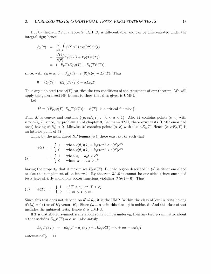
But by theorem 2.7.1, chapter 2, TSH, βψ is differentiable, and can be differentiated under theintegral sign; hence
β′ψ(θ) =d
dθ
∫ψ(t)c(θ) exp(θt)dν(t)
=c′(θ)
c(θ)Eθψ(T ) + Eθ(Tψ(T ))
= (−EθT )Eθψ(T ) + Eθ(Tψ(T ))
since, with ψ0 ≡ α, 0 = β′ψ0(θ) = c′(θ)/c(θ) + Eθ(T ). Thus
0 = β′ψ(θ0) = Eθ0(Tψ(T ))− αEθ0T.
Thus any unbiased test ψ(T ) satisfies the two conditions of the statement of our theorem. We willapply the generalized NP lemma to show that φ as given is UMPU.
Let
M ≡ {(Eθ0ψ(T ), Eθ0Tψ(T )) : ψ(T ) is a critical function}.
Then M is convex and contains {(u, uEθ0T ) : 0 < u < 1}. Also M contains points (α, v) withv > αEθ0T ; since, by problem 18 of chapter 3, Lehmann TSH, there exist tests (UMP one-sidedones) having β′(θ0) > 0. Likewise M contains points (α, v) with v < αEθ0T . Hence (α, αEθ0T ) isan interior point of M .
Thus, by the generalized NP lemma (iv), there exist k1, k2 such that
ψ(t) =
{1 when c(θ0)(k1 + k2t)e
θ0t < c(θ′)eθ′t
0 when c(θ0)(k1 + k2t)eθ0t > c(θ′)eθ
′t
=
{1 when a1 + a2t < ebt
0 when a1 + a2t > ebt(a)
having the property that it maximizes Eθ′ψ(T ). But the region described in (a) is either one-sidedor else the complement of an interval. By theorem 3.1.6 it cannot be one-sided (since one-sidedtests have strictly monotone power functions violating β′(θ0) = 0). Thus
ψ(T ) =
{1 if T < c1 or T > c2
0 if c1 < T < c2.(b)
Since this test does not depend on θ′ 6= θ0, it is the UMP (within the class of level α tests havingβ′(θ0) = 0) test of H4 versus K4. Since ψ0 ≡ α is in this class, ψ is unbiased. And this class of testincludes the unbiased tests. Hence ψ is UMPU.
If T is distributed symmetrically about some point a under θ0, then any test ψ symmetric abouta that satisfies Eθ0ψ(T ) = α will also satisfy
Eθ0Tψ(T ) = Eθ0(T − a)ψ(T ) + aEθ0ψ(T ) = 0 + aα = αEθ0T
automatically. 2

14 CHAPTER 6. TESTING
2.3 UMPU tests for families with nuisance parameter via conditioning
Definition 2.3 Let T be sufficient for PB ≡ {Pθ : θ ∈ ΘB}, and let PT ≡ {P Tθ : θ ∈ ΘB}. A testfunction φ is said to have Neyman structure with respect to T if
E(φ(X)|T ) = α a.s. PT .
Remark 2.4 If φ has Neyman structure with respect to T , then φ is SOB.
Proof. Eθφ(X) = EθE(φ(X)|T ) = Eθα = α for all θ ∈ ΘB. 2
Theorem 2.2 Let X be a random variable with distribution Pθ ∈ P = {Pθ : θ ∈ Θ}, and let Tbe sufficient for PB = {Pθ : θ ∈ ΘB}. Then all SOB tests have Neyman structure with respectT if and only if the family of distributions PT ≡ {P Tθ : θ ∈ ΘB} is boundedly complete: i.e. ifEPh(T ) = 0 for all P ∈ PT with h bounded, then h = 0 a.e. PT .
Proof. Suppose that PT is boundedly complete. Let φ be a SOB level α test; and defineψ(T ) ≡ E(φ(X)|T ). Now
Eθ(ψ(T )− α) = Eθ(E(φ(X)|T ))− α= Eθφ(X)− α = 0
for all θ ∈ ΘB, and since ψ(T )− α is bounded, the bounded completeness of PT implies ψ(T ) = αa.e. PT . Hence α = ψ(T ) = E(φ(X)|T ) a.e. PT , and φ has Neyman structure with respect to T .
Now suppose that all SOB tests have Neyman structure. Assume PT is not boundedly complete.Then there exists h such that |h| ≤some M with Eθh(T ) = 0 for all θ ∈ ΘB and h(T ) 6= 0 withprobability > 0 for some θ0 ∈ ΘB. Define φ(T ) ≡ ch(T ) + α where c ≡ {α ∧ (1 − α)}/M . Then0 ≤ φ(T ) ≤ 1 so φ is a critical function, and Eθφ(T ) = α for all θ ∈ ΘB, so that φ is SOB. ButE(φ(T )|T ) = φ(T ) 6= α with probability > 0 for the above θ0, so φ does not have Neyman structure.This is a contradiction, and hence it follows that indeed PT is boundedly complete. 2
Remark 2.5 Suppose that:(i) All critical functions φ have continuous power functions βφ.(ii) T is sufficient for PB = {Pθ : θ ∈ ΘB} and PT ≡ {P Tθ : θ ∈ ΘB} is boundedly complete.(Remark 2.3 says that (i) is always true for exponential families pθ(x) = c(θ) exp(
∑θjTj(x)); and
theorem 4.3.1, TSH, page 116, allows us to check (ii) for these same families.) Then all unbiasedtests are SOB and all SOB tests have Neyman structure. Thus if we can find a UMP Neymanstructure test φ0 and we can show that φ0 is unbiased, then φ0 is UMPU. Why is it easier to findUMP Neyman structure tests? Neyman structure tests are characterized by having conditionalprobability of rejection equal to α on each surface T = t. But the distribution on each such surfaceis independent of θ ∈ ΘB because T is sufficient for PT . Thus the problem has been reduced totesting a one parameter hypothesis for each fixed value of t; and in many problems we can easilyfind the most powerful test of this simple hypothesis.
Example 2.1 (Comparing two Poisson distributions).
Example 2.2 (Comparing two Binomial distributions).

2. UNBIASED TESTS; CONDITIONAL TESTS; PERMUTATION TESTS 15
Example 2.3 (Comparing two normal means when variances are equal).
Example 2.4 (Paired normals with nuisance shifts).
2.4 Application to general exponential families; k−parameter
Consider the exponential family P = {Pθ,ξ} given by
pθ,ξ(x) = c(θ, ξ) exp(θU(x) +
k∑i=1
ξiTi(x))
with respect to a σ−finite dominating measure µ on some subset of Rn where Θ is convex, hasdimension k + 1, and contains interior points θi, i = 1, 2.
Problems: Test
(1) H1 : θ ≤ θ0 versus K1 : θ > θ0;(2) H2 : θ ≤ θ1 or θ ≥ θ2 versus K2 : θ1 < θ < θ2;(3) H3 : θ1 ≤ θ ≤ θ2 versus K3 : θ < θ1 or θ2 < θ;(4) H4 : θ = θ0 versus K4 : θ 6= θ0.
Theorem 2.3 The following are UMPU tests for the hypothesis testing problems 1-4 respectively:(1) The test φ1 given by
φ1(x) =
1 if U > c(t)γ(t) if U = c(t)0 if if U < c(t)
where Eθ0(φ1(U)|T = t) = α is UMPU for H1 versus K1.(2) The test φ2 given by
φ2(x) =
1 if c1(t) < U < c2(t)γi(t) if U = ci(t)0 if if else
where Eθi(φ2(U)|T = t) = α, i = 1, 2, is UMPU for H2 versus K2.(3) The test φ3 given by
φ3(x) =
1 if U < c1(t) or U > c2(t)γi(t) if U = ci(t)0 if if else
where Eθi(φ3(U)|T = t) = α, i = 1, 2 is UMPU for H3 versus K3.(4) The test φ4 given by
φ4(x) =
1 if U < c1(t) or U > c2(t)γi(t) if U = ci(t)0 if if else
where Eθ0(φ4(U)|T = t) = α and Eθ0{Uφ4(U)|T = t} = αEθ0{U |T = t} is UMPU for H4 versusK4.
16 CHAPTER 6. TESTING
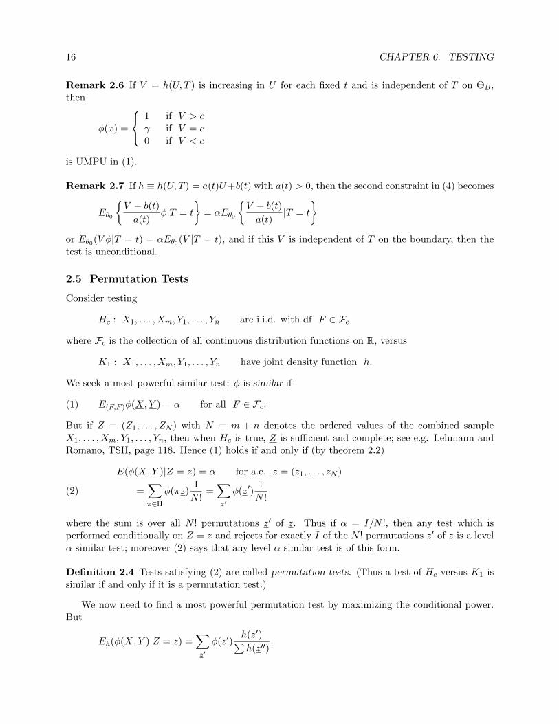
Remark 2.6 If V = h(U, T ) is increasing in U for each fixed t and is independent of T on ΘB,then
φ(x) =
1 if V > cγ if V = c0 if V < c
is UMPU in (1).
Remark 2.7 If h ≡ h(U, T ) = a(t)U+b(t) with a(t) > 0, then the second constraint in (4) becomes
Eθ0
{V − b(t)a(t)
φ|T = t
}= αEθ0
{V − b(t)a(t)
|T = t
}or Eθ0(V φ|T = t) = αEθ0(V |T = t), and if this V is independent of T on the boundary, then thetest is unconditional.
2.5 Permutation Tests
Consider testing
Hc : X1, . . . , Xm, Y1, . . . , Yn are i.i.d. with df F ∈ Fc
where Fc is the collection of all continuous distribution functions on R, versus
K1 : X1, . . . , Xm, Y1, . . . , Yn have joint density function h.
We seek a most powerful similar test: φ is similar if
E(F,F )φ(X,Y ) = α for all F ∈ Fc.(1)
But if Z ≡ (Z1, . . . , ZN ) with N ≡ m + n denotes the ordered values of the combined sampleX1, . . . , Xm, Y1, . . . , Yn, then when Hc is true, Z is sufficient and complete; see e.g. Lehmann andRomano, TSH, page 118. Hence (1) holds if and only if (by theorem 2.2)
E(φ(X,Y )|Z = z) = α for a.e. z = (z1, . . . , zN )
=∑π∈Π
φ(πz)1
N !=∑z′
φ(z′)1
N !(2)
where the sum is over all N ! permutations z′ of z. Thus if α = I/N !, then any test which isperformed conditionally on Z = z and rejects for exactly I of the N ! permutations z′ of z is a levelα similar test; moreover (2) says that any level α similar test is of this form.
Definition 2.4 Tests satisfying (2) are called permutation tests. (Thus a test of Hc versus K1 issimilar if and only if it is a permutation test.)
We now need to find a most powerful permutation test by maximizing the conditional power.But
Eh(φ(X,Y )|Z = z) =∑z′
φ(z′)h(z′)∑h(z′′)
.

2. UNBIASED TESTS; CONDITIONAL TESTS; PERMUTATION TESTS 17
Since the conditional densities under the composite null hypothesis and under the simple alternativeh are
p0(z′|z) =1
N !and p1(z′|z) =
h(z′)∑h(z′′)
, z′ ∈ {πz : π ∈ Π},
the conditional power is maximized by rejecting for large values of
p1(z′|z)p0(z′|z)
= Kzh(z′) with Kz =N !∑h(z′′)
.
Thus, at level α = I/N ! we reject if
h(z′) > c(z)
where c(z) is chosen so that we reject for exactly I of the N ! permutations z′ of z; or else we use arandomized version of such a test.
Example 2.5 Suppose now that we specify a particular alternative:
K1 :X1, . . . , Xm are i.i.d. N(θ1, σ
2)Y1, . . . , Yn are i.i.d. N(θ2, σ
2)
where θ1 < θ2 and σ2 are fixed constants. Then the similar test of Hc that is most powerful againthis simple K1 rejects H for those permutations z′ of z which lead to large values of
(2πσ2)−N/2 exp
{− 1
2σ2
(m∑1
(Xi − θ1)2 +
n∑1
(Yj − θ2)2
)},
or small values of
m∑1
(Xi − θ1)2 +
n∑1
(Yj − θ2)2
=m∑1
X2i +
n∑1
Y 2j +mθ2
1 + nθ22 − 2θ1
m∑i=1
Xi − 2θ2
n∑j=1
Yj ,
or large values of
θ1
m∑1
Xi + θ2
n∑1
Yj −mθ1 + nθ2
N(m∑1
Xi +n∑1
Yj)
=mn
N(θ2 − θ1)(Y −X),
or large values of
Y −X,
or large values of
θ1
m∑1
Xi + θ2
n∑1
Yj − θ1(m∑1
Xi +n∑1
Yj) = (θ2 − θ1)n∑j=1
Yj ,
18 CHAPTER 6. TESTING
or large values of √mnN (Y −X)√
1N−2
{∑Z2i −
(∑Zi)2
N − mnN (Y −X)2
}=
√mnN (Y −X)√
1N−2
{∑(Xi −X)2 +
∑(Yj − Y )2
} ≡ τ.Thus the most powerful similar test of Hc versus K1 is
φ(z′) =
{1 if τ > cα(z)0 if τ < cα(z)
where cα(z) is chosen so that exactly αN ! of the permutations z′ lead to rejection (if this is possible;if not we can use a randomized test). But we know that τ takes on at most
(Nm
)distinct values
according to each of the(Nm
)assignments zc of m of the zi’s to be Xi’s. Thus
φ(zc) =
{1 if τ(zc) > cα(z)0 if τ(zc) < cα(z)
(3)
where cα(z) is chosen so that exactly α(Nm
)of the assignments zc of m of the zi’s to be Xi’s leads
to rejection.Since the test (3) does not depend on which θ1 < θ2 or σ2 we started with, the test is actually
a UMP similar test of Hc versus K ≡ ∪θ1<θ2,σ2K1; i.e. different normal distributions with θ1 < θ2,σ2 unknown.
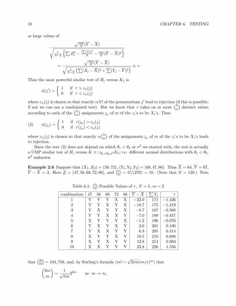
Example 2.6 Suppose that (X1, X2) = (56, 72), (Y1, Y2, Y3) = (68, 47, 86). Thus X = 64, Y = 67,Y − X = 3. Here Z = (47, 56, 68, 72, 86), and
(52
)= 5!/(2!3!) = 10. (Note that 5! = 120.) Note
Table 6.1:(
52
)Possible Values of τ , N = 5, m = 2
combination 47 56 68 72 86 Y −X∑Yj τ
1 Y Y Y X X −22.0 171 −1.4362 Y Y X Y X −18.7 175 −1.2193 Y X Y Y X −8.7 187 −0.5664 Y Y X X Y −7.0 189 −0.4575 X Y Y Y X −1.2 196 −0.0766 Y X Y X Y 3.0 201 0.1967 Y X X Y Y 6.3 205 0.4148 X Y Y X Y 10.5 210 0.6869 X Y X Y Y 13.8 214 0.90310 X X Y Y Y 23.8 226 1.556
that(
2010
)= 184, 756, and, by Stirling’s formula (m! ∼
√2πm(m/e)m) that(
2m
m
)∼ 1√
πm22m as m→∞,

2. UNBIASED TESTS; CONDITIONAL TESTS; PERMUTATION TESTS 19
so the exact permutation test is difficult computationally for all but small sample sizes. Butsampling from the permutation distribution is always possible.
Remark 2.8 We will call the present test “reject if τ > cα(z)” the permutation t - test; it is theUMP similar test of Hc versus K specified above. If we consider the smaller null hypothesis
HG : X1, . . . , Xm, Y1, . . . , Yn i.i.d. N(θ, σ2) with θ, σ2 unknown,
then we recall that the classical t -test “reject if τ > tm+n−2,α” is the UMPU test of HG versus K.
The classical t−test has greater power than the permutation t−test for HG; but is not a similartest of Hc. If we could show that for a.e. z the numbers
cα(z) and tm+n−2,α
where just about equal, then the classical t−test and the permutation t−test would be almostidentical.
Theorem 2.4 If F ∈ Fc has EF |X|2 <∞ and if 0 < lim inf(m/N) ≤ lim sup(m/N) < 1, then
cα(z)→ zα
where P (N(0, 1) > zα) = α. Since we also know that tm+n−2,α → zα, it follows that cα(z) −tm+n−2,α → 0.
Proof. Let an urn contain balls numbered z1, . . . , zN . Let Y1, . . . , Yn denote the numbers on nballs drawn without replacement. let z = N−1
∑Ni=1 zi, σ
2z = N−1
∑N1 (zi − z)2, m = N − n. Then
EY = z, and σ2N ≡ V ar(Y ) =
(1− n− 1
N − 1
)σ2z
n.
Moreover, by the Wald - Wolfowitz - Noether - Hajek finite sampling CLT
Y − zσN
→d N(0, 1)
as long as the Noether condition
ηN ≡max1≤i≤N |zi − z|2∑N
i=1 |zi − z|2→ 0(a)
holds.
Now rewrite the permutation t− statistic τ : note that
Y −X = Y − 1
m
m∑1
Xi −1
m
n∑1
Yi +n
mY
=N
m(Y − z),

20 CHAPTER 6. TESTING
and hence
τ =
√mnN (Y −X)√
1N−2
{∑Z2i −
(∑Zi)2
N − mnN (Y −X)2
}
=
√NN−1
Y−z√1n
(1− n−1N−1
)√NN−2σ
2z − 1
N−2NN−1
(Y−z)21n
(1− n−1N−1
)
=
√N − 2
N − 1
(Y − z)/σN√1− 1
N−1(Y−z)2σ2N
→d 1 · Z√1− 0 · Z2
= Z ∼ N(0, 1)
if
Y − zσN
→d Z ∼ N(0, 1)
in probability or, better yet, almost surely; i.e. if
P
(Y − zσN
≤ t∣∣∣Z = z
)→ Φ(t)
in probability or almost surely. But this holds under the present hypotheses in view of the finite -sampling CLT 2.5 which follows, if we can show that
ηN →a.s. 0(b)
where ηN is key quantity in the Noether condition (a). To accomplish this note that even underthe alternative hypothesis F 6= G and EF |X|2 <∞, EG|Y |2 <∞,
1
N
N∑i=1
(Zi − Z)2 =1
N
{N∑i=1
Z2i −NZ
2
}
=(m− 1)
NS2X +
(n− 1)
NS2Y
→a.s. λσ2X + (1− λ)σ2
Y ≥ min{σ2X , σ
2Y } > 0
for any subsequence N → ∞ for which λN ≡ m/N → λ, and hence the denominator of ηN(divided by N) has a positive limit inferior almost surely. To see that the numerator convergesalmost surely to zero, first recall that max1≤i≤n |Xi|/n →a.s. 0 if and only if EF |X1| < ∞. Hencemax1≤i≤n |Xi|2/n →a.s. 0 if and only if EF |X1|2 < ∞. Thus we rewrite the numerator divided byN as
1
Nmaxi≤N|Zi − Z|2 ≤ 2
N
{maxi≤N|Zi|2 + Z
2}
≤ 2
N
{max{max
i≤m|Xi|2, max
j≤n|Yj |2}+
(mNX +
n
NY)2}
≤ 2 max{ 1
mmaxi≤m|Xi|2,
1
nmaxj≤n|Yj |2}+
2
N
(mNX +
n
NY)2
→a.s. 0 + 0.

2. UNBIASED TESTS; CONDITIONAL TESTS; PERMUTATION TESTS 21
Hence (b) holds (even under the alternative if EFX2 <∞ and EGY
2 <∞). 2
Theorem 2.5 (Wald - Wolfowitz - Noether - Hajek finite - sampling central limit theorem). If0 < lim inf(m/N) ≤ lim sup(m/N) < 1, then
Y − zσN
→d Z ∼ N(0, 1) as N →∞
if and only if
ηN ≡max1≤i≤N |zi − z|2∑N
i=1 |zi − z|2→ 0 as N →∞.(4)
Moreover,
supt
∣∣∣P (Y − zσN
≤ t)− Φ(t)
∣∣∣ ≤ 5
(N
m ∧ nηN
)1/4
for all N ≥ 1.
Proof. See Hajek, Ann. Math. Statist. 32, 506 - 523. For still better rates under strongerconditions, see Bolthausen (1984). 2

22 CHAPTER 6. TESTING
3 Invariance in Testing; Rank Methods
3.1 Notation and Basic Results
Let (X ,A, Pθ) be a probability space for all θ ∈ Θ, and suppose θ 6= θ′ implies Pθ 6= Pθ′ . Weobserve X ∼ Pθ.
Suppose that g : X → X is one-to-one, onto X , and measurable, and suppose that the distri-bution of gX when X ∼ Pθ is some Pθ′ = Pgθ; that is
Pθ(gX ∈ A) = Pgθ(X ∈ A) for all A ∈ A,(1)
or equivalently
Pθ(g−1A) = Pgθ(A) for all A ∈ A;
or, equivalently,
Pθ(A) = Pgθ(gA) for all A ∈ A.
Hence
Eθh(g(X)) = Egθh(X).(2)
Suppose that gΘ = Θ.Let G denote a group of such tranformations g. We want to test H : θ ∈ ΘH versus K : θ ∈ ΘK .
Proposition 3.1 G is a group of one-to-one transformations of Θ onto Θ and is homomorphic toG.
Proof. Suppose that gθ1 = gθ2. Then Pθ1 = Pθ2 by (1). Thus θ1 = θ2 by assumption. Thusg ∈ G is one-to-one.
Closure, associativity, and identity are easy.If X ∼ Pθ, then g1X ∼ Pg1θ, and (g2 ◦g1)X = g2 ◦ (g1X) ∼ Pg2◦g1θ, while (g2 ◦g1)X ∼ Pg2◦g1 , so
g2 ◦ g1 = g2 ◦ g1. If X ∼ Pθ, then g−1X ∼ Pg−1θ
, so g ◦ g−1X ∼ Pg◦ ¯g−1θ, while g ◦ g−1X = X ∼ Pθ,so g ◦ g−1 = e; thus g−1 = g−1, and G is a group. 2
Definition 3.1 A group of one-to-one transformations of X onto X is said to leave the testingproblem H versus K invariant provided gΘ = Θ and gΘH = ΘH for all g ∈ G.
3.2 Orbits and maximal invariants
Definition 3.2 x1 ∼ x2mod(G) if x2 = g(x1) for some g ∈ G.
Proposition 3.2 ∼ is an equivalence relation.
Proof. Reflexive: x1 ∼ x1 since x1 = e(x1).Symmetric: g(x1) = x2 implies g−1(x2) = x1.Transitive: x1 ∼ x2 and x2 ∼ x3 implies x1 ∼ x3 since g1(x1) = x2 and g2(x2) = x3 implies(g2 ◦ g1)(x1) = x3. 2

3. INVARIANCE IN TESTING; RANK METHODS 23
Definition 3.3 The equivalence classes of ∼ are called the orbits of G. Thus orbit(x) = {g(x) :g ∈ G}. A function φ defined on the sample space X is invariant if φ(g(x)) = φ(x) for all x ∈ Xand all g ∈ G.
Proposition 3.3 A test function φ is invariant if and only if φ is constant on each orbit of G.
Proof. This follows immediately from the definitions. 2
Definition 3.4 A measurable function T : X → Rk for some k is a maximal invariant for G (orGMI), if T is invariant and T (x1) = T (x2) implies x1 ∼ x2. That is, T is constant on the orbits ofG and takes on distinct values on distinct orbits.
Theorem 3.1 Let T be a GMI. Then φ is invariant if and only if there exists a function h suchthat φ(x) = h(T (x)) for all x ∈ X .
Proof. Suppose that φ(x) = h(T (x)). Then
φ(gx) = h(T (gx)) = h(T (x)) = φ(x),
so φ is invariant.On the other hand, suppose that φ is G−invariant. Then T (x1) = T (x2) implies x1 ∼ x2 implies
g(x1) = x2 for some g ∈ G. Thus φ(x2) = φ(gx1) = φ(x1); that is, φ is constant on the orbit. Itfollows that φ is a function of T . 2
3.3 Examples
Example 3.1 (Translation group). Suppose that X = Rn and G = {g : gx = x + c1, c ∈ R}.Then T (x) = (x1 − xn, . . . , xn−1 − xn) is a GMI.Proof: Clearly T is invariant. Suppose that T (x) = T (x∗). Then xi = x∗i − (x∗n − xn) for i =1, . . . , n− 1, and this holds trivially for i = n. Thus x∗ = g(x) = x+ c1 with c = (x∗n − xn).
Example 3.2 (Scale group). Suppose that X = {x ∈ Rn : xn 6= 0}, and G = {g : gx = cx, c ∈R \ {0}}. Then T (x) = (x1/xn, . . . , xn−1/xn) is a GMI.Proof: Clearly T is invariant. Suppose that T (x) = T (x∗). Then x∗i = (x∗n/xn)xi for i = 1, . . . , n−1,this holds trivially for i = n. Thus x∗ = g(x) = cx with c = (x∗n/xn).
Example 3.3 (Orthogonal group). Suppose that X = Rn and G = {g : gx = Γx, Γ an n ×n orthogonal matrix}. Then T (x) = xTx =
∑ni=1 x
2i is a GMI.
Proof: T (gx) = xTΓTΓx = xTx, so T is invariant. Suppose that T (x) = T (x∗). Then there existsΓ = Γx,x∗ such that x∗ = Γx.
Example 3.4 (Permutation group). Suppose that X = Rn \ {ties}, and G = {g : g(x) = πx =(xπ(1), . . . , xπ(n)) for some permutation π = (π(1), . . . , π(n)) of {1, . . . , n}. Note that #(G) = n!.Then T (x) = (x(1), . . . , x(n)) ≡ x(·), the vector of ordered x’s is a GMI.Proof. T (gx) = T (πx) = x(·) = T (x), so T is invariant. Moreover, if T (x∗) = T (x), then x∗ = πxfor some π ∈ Π, so T is maximal.

24 CHAPTER 6. TESTING
Example 3.5 (Rank transformation group). Suppose that X = {x ∈ Rn : xi 6= xj for all i 6=j} = Rn \ {ties}, and G = {g : g(x) = (f(x1), . . . , f(xn)), f continuous and strictly increasing}.Then T (x) ≡ r = (r1, . . . , rn) where ri ≡ #{j ≤ n : xj ≤ xi} denotes the rank of xi (amongx1, . . . , xn).Proof: T is clearly invariant. If T (x∗) = T (x), then, relabeling if necessary, we have a picture asfollows:
Example 3.6 (Sign group). Suppose that X = Rn and that G = {g, e}n where g(x) = −x ande(x) = x. Then T (x) = (|x1|, . . . , |xn|) is a GMI.
Example 3.7 (Affine group). Suppose that X = {x ∈ Rn : xn−1 6= xn} and that G = {g : g(x) =ax+ b1 with a 6= 0, b ∈ R}. Then
T (x) =
(x1 − xnxn−1 − xn
, . . . ,xn−2 − xnxn−1 − xn
)is a GMI. Note that
T (x) =
(x1 − xs
, . . . ,xn − xs
)is also a GMI (on X ≡ {x ∈ Rn : s > 0} where s2 ≡ n−1
∑ni=1(xi − x)2).
Remark 3.1 In the previous example G = G2⊕G1 = scale⊕translation = {g2◦g1 : g1 ∈ G1, g2 ∈G2}. Then Y = (x1−xn, x2−xn, . . . , xn−1−xn) is a G1− MI. In the space of the G1−MI we haveZ = (y1/yn−1, . . . , yn−2/yn−1) is a G2−MI. Thus Z is the GMI. If this works, it is OK; see theorem2 on page 218 of TSH. But it doesn’t always work. When G = G2 ⊕ G1, it does work if G1 is anormal subgroup of G. [Recall that G1 is a normal subgroup of G if and only if gG1g
−1 = G1 forall g ∈ G.]
Example 3.8 (Signed rank transformation group). Suppose that X = RN \{ties} as in example 3.5(but with N instead of n), but now let and
G = {g : g(x) = (f(x1), . . . , f(xN )), f is odd, continuous, and strictly increasing}.
Then T (x) = (r, s) = (r1, . . . , rm, s1, . . . , sn) where r1, . . . , rm denote the ranks of |xi1 |, . . . , |xim |among |x1|, . . . , |xN | and s1, . . . , sn denote the rank of |xj1 |, . . . , |xjn | among |x1|, . . . , |xN | and wherexi1 , . . . , xim < 0 < xj1 , . . . , xjn .Proof: T is clearly invariant. To show maximal invariance, the picture is much as in example 3.5,but with the function f being odd; see Lehmann TSH pages 316 - 317.
3. INVARIANCE IN TESTING; RANK METHODS 25
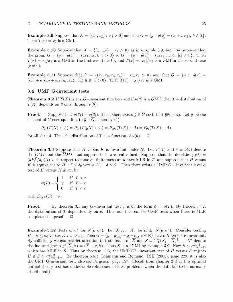
Example 3.9 Suppose that X = {(x1, x2) : x2 > 0} and that G = {g : g(x) = (x1+b, x2), b ∈ R}.Then T (x) = x2 is a GMI.
Example 3.10 Suppose that X = {(x1, x2) : x2 > 0} as in example 3.9, but now suppose thatthe group G = {g : g(x) = (cx1, cx2), c > 0} or G = {g : g(x) = (cx1, |c|x2), |c| 6= 0}. ThenT (x) = x1/x2 is a GMI in the first case (c > 0), and T (x) = |x1|/x2 is a GMI in the second case(c 6= 0).
Example 3.11 Suppose that X = {(x1, x2, x3, x4) : x3, x4 > 0} and that G = {g : g(x) =(cx1 + a, cx2 + b, cx3, cx4), a, b ∈ R, c > 0}. Then T (x) = x3/x4 is a GMI.
3.4 UMP G-invariant tests
Theorem 3.2 If T (X) is any G−invariant function and if ν(θ) is a GMI, then the distribution ofT (X) depends on θ only through ν(θ).
Proof. Suppose that ν(θ1) = ν(θ2). Then there exists g ∈ G such that gθ1 = θ2. Let g be theelement of G corresponding to g ∈ G. Then by (1)
Pθ1(T (X) ∈ A) = Pθ1(T (gX) ∈ A) = Pgθ1(T (X) ∈ A) = Pθ2(T (X) ∈ A)
for all A ∈ A. Thus the distribution of T is a function of ν(θ). 2
Theorem 3.3 Suppose that H versus K is invariant under G. Let T (X) and δ ≡ ν(θ) denotethe GMI and the GMI; and suppose both are real-valued. Suppose that the densities pδ(t) =(dP Tδ /dµ)(t) with respect to some σ−finite measure µ have MLR in T ; and suppose that H versusK is equivalent to H1 : δ ≤ δ0 versus K1 : δ > δ0. Then there exists a UMP G− invariant level αtest of H versus K given by
ψ(T ) =
1 if T > cγ if T = c0 if T < c
with Eδ0ψ(T ) = α.
Proof. By theorem 3.1 any G−invariant test φ is of the form φ = ψ(T ). By theorem 3.2,the distribution of T depends only on δ. Thus our theorem for UMP tests when there is MLRcompletes the proof. 2
Example 3.12 Tests of σ2 for N(µ, σ2). Let X1, . . . , Xn be i.i.d. N(µ, σ2). Consider testingH : σ ≤ σ0 versus K : σ > σ0. Then G = {g : g(x) = x+ c1, c ∈ R} leaves H versus K invariant.By sufficiency we can restrict attention to tests based on X and S ≡
∑n1 (Xi −X)2. let G∗ denote
the induced group g∗(X,S) = (X + c, S). Thus S is a G∗MI by example 3.9. Now S ∼ σ2χ2n−1,
which has MLR in S. Thus by theorem 3.3, the UMP G∗−invariant test of H versus K rejectsH if S > σ2
0χ2n−1,α. By theorem 6.5.3, Lehmann and Romano, TSH (2005), page 229, it is also
the UMP G-invariant test; also see Ferguson, page 157. (Recall from chapter 2 that this optimalnormal theory test has undesirable robustness of level problems when the data fail to be normallydistributed.)
26 CHAPTER 6. TESTING
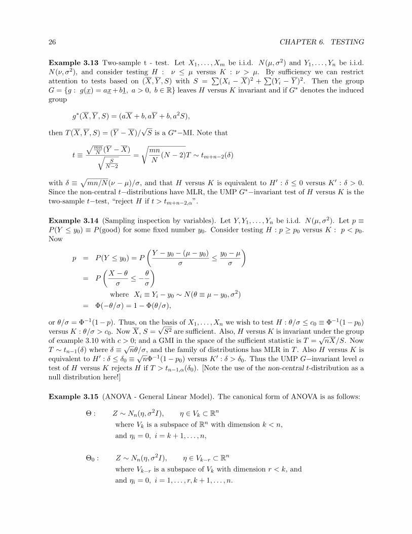
Example 3.13 Two-sample t - test. Let X1, . . . , Xm be i.i.d. N(µ, σ2) and Y1, . . . , Yn be i.i.d.N(ν, σ2), and consider testing H : ν ≤ µ versus K : ν > µ. By sufficiency we can restrictattention to tests based on (X,Y , S) with S =
∑(Xi − X)2 +
∑(Yi − Y )2. Then the group
G = {g : g(x) = ax+ b1, a > 0, b ∈ R} leaves H versus K invariant and if G∗ denotes the inducedgroup
g∗(X,Y , S) = (aX + b, aY + b, a2S),
then T (X,Y , S) = (Y −X)/√S is a G∗−MI. Note that
t ≡√
mnN (Y −X)√
SN−2
=
√mn
N(N − 2)T ∼ tm+n−2(δ)
with δ ≡√mn/N(ν − µ)/σ, and that H versus K is equivalent to H ′ : δ ≤ 0 versus K ′ : δ > 0.
Since the non-central t−distributions have MLR, the UMP G∗−invariant test of H versus K is thetwo-sample t−test, “reject H if t > tm+n−2,α”.
Example 3.14 (Sampling inspection by variables). Let Y, Y1, . . . , Yn be i.i.d. N(µ, σ2). Let p ≡P (Y ≤ y0) ≡ P (good) for some fixed number y0. Consider testing H : p ≥ p0 versus K : p < p0.Now
p = P (Y ≤ y0) = P
(Y − y0 − (µ− y0)
σ≤ y0 − µ
σ
)= P
(X − θσ
≤ − θσ
)where Xi ≡ Yi − y0 ∼ N(θ ≡ µ− y0, σ
2)
= Φ(−θ/σ) = 1− Φ(θ/σ),
or θ/σ = Φ−1(1− p). Thus, on the basis of X1, . . . , Xn we wish to test H : θ/σ ≤ c0 ≡ Φ−1(1− p0)versus K : θ/σ > c0. Now X, S =
√S2 are sufficient. Also, H versus K is invariant under the group
of example 3.10 with c > 0; and a GMI in the space of the sufficient statistic is T =√nX/S. Now
T ∼ tn−1(δ) where δ ≡√nθ/σ, and the family of distributions has MLR in T . Also H versus K is
equivalent to H ′ : δ ≤ δ0 ≡√nΦ−1(1− p0) versus K ′ : δ > δ0. Thus the UMP G−invariant level α
test of H versus K rejects H if T > tn−1,α(δ0). [Note the use of the non-central t-distribution as anull distribution here!]
Example 3.15 (ANOVA - General Linear Model). The canonical form of ANOVA is as follows:
Θ : Z ∼ Nn(η, σ2I), η ∈ Vk ⊂ Rn
where Vk is a subspace of Rn with dimension k < n,
and ηi = 0, i = k + 1, . . . , n,
Θ0 : Z ∼ Nn(η, σ2I), η ∈ Vk−r ⊂ Rn
where Vk−r is a subspace of Vk with dimension r < k, and
and ηi = 0, i = 1, . . . , r, k + 1, . . . , n.

3. INVARIANCE IN TESTING; RANK METHODS 27
We let
G1 ≡ {g1 : g1z = (z1, . . . , zr, zr+1 + ∆r+1, . . . , zk + ∆k, zk+1, . . . , zn), with ∆i ∈ R} ,
G2 =
{g2 : g2z = (z∗1 , . . . , z
∗r , zr+1, . . . , zk, zk+1, . . . , zn),
(z∗1 , . . . , z∗r ) an orthogonal transformation of (z1, . . . , zr)
},
G3 =
{g3 : g3z = (z1, . . . , zr, zr+1, . . . , zk, z
∗k+1, . . . , z
∗n),
(z∗k+1, . . . , z∗n) an orthogonal transformation of (zk+1, . . . , zn)
},
G4 = {g4 : g4z = cz, where c 6= 0};
and, finally
G ≡ G4 ⊕G3 ⊕G2 ⊕G1 ≡ {g4 ◦ g3 ◦ g2 ◦ g1 : gi ∈ Gi, i = 1, . . . , 4}.
Then H versus K is invariant under G.Now T1(z) = (z1, . . . , zr, zk+1, . . . , zn) is a G1MI.
In the space of the G1MI, a G2MI is T2(z) = (∑r
i=1 z2i , zk+1, . . . , zn).
In the space of the G2 ⊕G1MI, a G3MI is T3(z) = (∑r
i=1 z2i ,∑n
i=k+1 z2i ).
In the space of the G3 ⊕G2 ⊕G1MI, a G4MI is T (z) = ((n− k)/r)(∑r
1 z2i /∑n
k+1 z2i
).
Now T (z) is a GMI; thus any G−invariant test function for H versus K is a function of T (z)by theorem 3.1. Similarly,
(σ2, η1, . . . , ηr) is a G1MI;
(σ2,r∑i=1
η2i ) is a G2 ⊕G1MI; and a G3 ⊕G2 ⊕G1MI;
and
δ2 ≡ λ2 =
∑ri=1 η
2i
σ2is a GMI.
Thus the distribution of any invariant test depends only on δ2.Now T ∼ Fr,n−k(δ2), which has MLR in T . Also, H versus K is equivalent to H ′ : δ = 0 versus
K ′ : δ > 0. Thus the UMP G−invariant test of H versus K rejects H when T > Fr,n−k,α.
Reduction to canonical form
The above analysis has been developed for the linear model in canonical form. Now the questionis: how do we reduce a model stated in a more usual way to the canonical form? Suppose that
X ∼ Nn(ξ, σ2I)
where ξ ≡ EX = Aθ ∈ L, where A is a (known) n × k matrix of rank k, θ is a k × 1 vector of(unknown) parameters, and L is the k−dimensional subspace of Rn spanned by the columns of thematrix A. Let B be a given r × k matrix, and consider testing
H : Bθ = 0 or ξ ∈ L1
where L1 is a (k − r)−dimensional subspace of Rn.To transform this form of the testing problem to canonical form, let T be an n× n orthogonal
matrix with:
(i) the last n− k rows of T are orthogonal to L; i.e. orthogonal to the columns of A.

28 CHAPTER 6. TESTING
(ii) the rows r + 1, . . . , k of T span L1.
Then set Z = TX. We compute
η ≡ EZ = TAθ = Tξ,
and note that:
(a) ηk+1 = · · · = ηn = 0 always by (i).
(b) η1 = · · · = ηr = 0 under H by (ii) since the first r rows of T are orthogonal to L1.
Now we will re-express the F−statistic we have derived in terms of the X’s:
S2(η) ≡n∑i=1
(Zi − ηi)2 =k∑i=1
(Zi − ηi)2 +n∑
i=k+1
Z2i
≥n∑
i=k+1
Z2i
by taking ηi = ηi = Zi, i = 1, . . . , k. But since T is orthogonal, η = Tξ, and Z = TX,
S2(η) = ‖Z − η‖2 = (Z − η)T (Z − η)(3)
= (X − ξ)T (X − ξ) =
n∑i=1
(Xi − ξi)2(4)
so that
minξ∈L
n∑i=1
(Xi − ξi)2 =n∑i=1
(Xi − ξi)2 =n∑
i=k+1
Z2i(5)
where ξ is the Least Squares (LS) estimator of ξ under ξ = Aθ ∈ L. Similarly, under H : ξ ∈ L1
(or η1 = · · · = ηr = 0 in the canonical form),
S2(η) =r∑i=1
Z2i +
k∑i=r+1
(Zi − ηi)2 +n∑
i=k+1
Z2i
≥r∑i=1
Z2i +
n∑k+1
Z2i
by taking ηi = ˆηi = Zi for i = r + 1, . . . , k, and hence by (4)
minξ∈L1
n∑i=1
(Xi − ξi)2 ≡n∑i=1
(Xi − ˆξi)
2 =r∑i=1
Z2i +
n∑i=k+1
Z2i(6)
whereˆξ is the least squares estimate of ξ under the hypothesis ξ ∈ L1. Combining (5) and (6)
yields
r∑i=1
Z2i =
n∑i=1
(Xi − ˆξi)
2 −n∑i=1
(Xi − ξi)2;
3. INVARIANCE IN TESTING; RANK METHODS 29
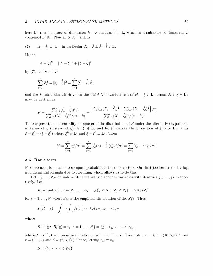
here L1 is a subspace of dimension k − r contained in L, which is a subspace of dimension kcontained in Rn. Now since X − ξ ⊥ L
X − ξ ⊥ L; in particular, X − ξ ⊥ ξ − ˆξ ∈ L.(7)
Hence
‖X − ˆξ‖2 = ‖X − ξ‖2 + ‖ξ − ˆ
ξ‖2
by (7), and we have
r∑i=1
Z2i = ‖ξ − ˆ
ξ‖2 =
n∑i=1
(ξi − ˆξi)
2,
and the F−statistics which yields the UMP G−invariant test of H : ξ ∈ L1 versus K : ξ /∈ L1
may be written as
F =
∑ni=1(ξi − ˆ
ξi)2/r∑n
i=1(Xi − ξi)2/(n− k)=
{∑ni=1(Xi − ˆ
ξi)2 −
∑ni=1(Xi − ξi)2
}/r∑n
i=1(Xi − ξi)2/(n− k).
To re-express the noncentrality parameter of the distribution of F under the alternative hypothesisin terms of ξ (instead of η), let ξ ∈ L, and let ξ0 denote the projection of ξ onto L1: thus
ξ = ξ0 + (ξ − ξ0) where ξ0 ∈ L1 and ξ − ξ0 ⊥ L1. Then
δ2 =r∑i=1
η2i /σ
2 =n∑i=1
{ξi(ξ)− ˆξi(ξ)}2/σ2 =
n∑i=1
{ξi − ξ0i }2/σ2.
3.5 Rank tests
First we need to be able to compute probabilities for rank vectors. Our first job here is to developa fundamental formula due to Hoeffding which allows us to do this.
Let Z1, . . . , ZN be independent real-valued random variables with densities f1, . . . , fN respec-tively. Let
Ri ≡ rank of Zi in Z1, . . . , ZN = #{j ≤ N : Zj ≤ Zi} = NFN (Zi)
for i = 1, . . . , N where FN is the empirical distribution of the Zi’s. Thus
P (R = r) =
∫· · ·∫Sf1(z1) · · · fN (zN )dz1 · · · dzN
where
S ≡ {z : Ri(z) = ri, i = 1, . . . , N} = {z : zd1 < · · · < zdN }
where d = r−1, the inverse permutation, r ◦d = r ◦ r−1 = e. (Example: N = 3; z = (10, 5, 8). Thenr = (3, 1, 2) and d = (2, 3, 1).) Hence, letting zdi ≡ vi,
S = {V1 < · · · < VN},

30 CHAPTER 6. TESTING
and
P (R = r) =
∫· · ·∫v1<···<vN
f1(vr1) · · · fN (vrN )
N !h(vr1) · · ·h(vrN )N !h(v1) · · ·h(vN )dv
=1
N !Ef1(V(r1)) · · · fN (V(rN ))
h(V(r1)) · · ·h(V(rN ))
where V(1) < · · · < V(N) are the order statistics of a sample of size N from h. This formula is oneversion of Hoeffding’s formula.
Of course, sometimes direct calculation succeeds immediately. Here are two simple, but impor-tant, examples:
Example 3.16 Suppose that Fi = F∆i with ∆i > 0, i = 1, . . . , N and F continuous. Then
P (R = e) = P (X1 < · · · < XN ) =
∫· · ·∫x1<···<xN
N∏i=1
dF∆i(xi)
=
∫· · ·∫
0≤u1≤···≤uN≤1
N∏i=1
∆iu∆i−1i dui
=
∫· · ·∫
0≤u2≤···≤uN≤1
N∏i=3
∆iu∆i−1i ∆2u
∆1+∆2−12 du2 · · · duN
= · · · =
N∏i=1
∆i∑ij=1 ∆j
.
This yields any probability P (R = r), r ∈ Π, by relabeling:
P (R = r) =
N∏i=1
∆di∑ij=1 ∆dj
.
Example 3.17 (Proportional hazards alternative). Similarly, suppose that (1 − Fi) = (1 − F )∆i
with ∆i > 0, i = 1, . . . , N and F continuous; this is equivalent to Λi ≡ − log(1−Fi) = ∆i{− log(1−F )} = ∆iΛ, the proportional hazards model. Then
P (R = e) = P (X1 < · · · < XN ) =
∫· · ·∫x1<···<xN
N∏i=1
d{1− (1− F (xi))∆i}
=
∫· · ·∫
0≤u1≤···≤uN≤1
N∏i=1
∆i(1− ui)∆i−1dui
= · · · =N∏i=1
∆i∑Nj=i ∆j
.
This yields any probability P (R = r), r ∈ Π, by relabeling:
P (R = r) =
N∏i=1
∆di∑Nj=i ∆dj
.

3. INVARIANCE IN TESTING; RANK METHODS 31
Now suppose that X1, . . . , Xm are i.i.d. F and Y1, . . . , Yn are i.i.d. G, F,G ∈ Fc; and let Gdenote the group of all strictly increasing continuous transformations of the real line onto itself,example 3.5.
Proposition 3.4A. The two-sample problem of testing H : F = G versus K : F <s G, F,G ∈ Fc, is invariantunder G.B. The rank vector R is a G−MI.C. ψ(u) = G ◦ F−1(u) is a G−MI.D. The ordered Y ranks Q1 < · · · < Qn are sufficient for R; Qi ≡ NHN (G−1
n (i/n)), i = 1, . . . , n.E. Hoeffding’s formula: suppose that F and G have densities f and g respectively, and thatf(x) = 0 implies g(x) = 0. Then
P (Q = q) =1(Nn
)Ef
n∏j=1
g(V(qj))
f(V(qj))
where V(1) < · · · < V(N) are the order statistics of a sample of size N from F . Furthermore, thisprobability may be rewritten as
P (Q = q) =1(Nn
)E
n∏j=1
ψ′(U(qj))
where U(1) < · · · < U(N) are the order statistics of a sample of N Uniform(0, 1) random variables.
Proof. Statements A - C follow easily from the preceding development. To prove E, wespecialize Hoeffding’s formula by taking fi = f for i = 1, . . . ,m, fi = g for i = m + 1, . . . , N , andh = f . Then
P (R = r) =1
N !EF
n∏j=1
g
f(V(rm+j))
=1
N !EF
n∏j=1
g
f(V(qj))
.
Hence
P (Q = q) =∑
r: q(r)=q
P (R = r) =1
N !EF
n∏j=1
g
f(V(qj))
∑r: q(r)=q
1
=m!n!
N !EF
n∏j=1
g
f(V(qj))
.
Note that the claimed sufficiency of Q for R in D follows from these computations.To see the second formula, note that ψ′(u) = (g/f)(F−1(u)), and that
(F−1(U(1), . . . , F−1(U(N)))
d= (V(1), . . . , V(N)).
2
Here are several applications of Hoeffding’s formula: we use the preceding results to find locallymost powerful rank tests in several different two-sample testing problems: location, scale, andLehmann alternatives of the proportional hazards type.

32 CHAPTER 6. TESTING
Proposition 3.5 (Locally most powerful rank test for location). Suppose that F has an absolutelycontinuous density f for which
∫|f ′(x)|dx < ∞. Then the locally most powerful rank test of
H : F = G versus K : G = F (· − θ) with θ > 0 is of the form
φ(q) =
1 if SN ≡
∑nj=1EF
(−f ′
f (V(qj)))> kα
γ if SN = kα0 if SN < kα
where V(1) < · · · < V(N) are the order statistics in a sample of size N from F .
Proof. For a rank test, φ = φ(Q), we want to maximize the slope of the power function atθ = 0: i.e. to maximize the slope at θ = 0 of
βφ(θ) = Eθφ(Q) =∑q
φ(q)Pθ(Q = q).
To do this we clearly want to find those q for which
d
dθPθ(Q = q)
∣∣∣θ=0
is large. But, by using proposition 3.4 and differentiation under the expectation (which can bejustified by the assumption that
∫|f ′(x)|dx <∞),
d
dθPθ(Q = q)
∣∣∣θ=0
=d
dθ
1(Nn
)EF { n∏i=1
f(V(qj) − θ)f(V(qj))
}∣∣∣θ=0
=1(Nn
)EF { d
dθ
n∏i=1
f(V(qj) − θ)f(V(qj))
∣∣∣θ=0
}
=1(Nn
)EF−
n∑j=1
f ′
f(V(qj))
since
d
dθ
n∏j=1
f(xj − θ)f(xj)
=n∑k=1
n∏j=1,j 6=k
f(xj − θ)f(xj)
∣∣∣θ=0
{−f′(xk − θ)f(xk)
∣∣∣θ=0
}
= −n∑k=1
f ′
f(xk).
2
Example 3.18 If F is N(µ, σ2), then without loss (by the monotone transformation g(X) =(X−µ)/σ, we may take F = Φ, the standardN(0, 1) distribution function. Then−(f ′/f)(x) = x, soE{(−f ′/f)(V(i))} = E(Z(i)) where Z(1) < · · · < Z(N) are the order statistics of N standard normal(N(0, 1)) random variables, and SN =
∑nj=1E(Z(qj)). Note that E(Z(i)) may be approximated by
Φ−1(i/(N + 1)), or by Φ−1((3i− 1)/(3N + 1)).

3. INVARIANCE IN TESTING; RANK METHODS 33
Example 3.19 If F is logistic, f(x) = e−x/(1 + e−x)2, then f = F (1− F ), and −f ′/f = 2F − 1.
Since F (V(i))d= U(i) where U1, . . . , UN are uniform(0, 1) random variables with EU(i) = i/(N + 1),
the LMPRT of F versus G = F (· − θ) rejects H for large values of SN =∑n
j=1Qj ; this is theWilcoxon statistic.
Proposition 3.6 (Locally most powerful rank test for scale). Suppose that F has an absolutelycontinuous density f for which
∫|xf ′(x)|dx < ∞. Then the locally most powerful rank test of
H : F = G versus K : G = F (·/θ) with θ > 1 is of the form
φ(q) =
1 if SN ≡
∑nj=1 aN (qj) > kα
γ if SN = kα0 if SN < kα
where
aN (i) ≡ EF {−1− V(i)f ′
f(V(i))}
and V(1) < · · · < V(N) are the order statistics in a sample of size N from F .
Example 3.20 If f(x) = e−x1[0,∞)(x), then (f ′/f)(x) = −1, and hence aN (i) = EF {−1 + V(i)} =EF {V(i) − 1} where V(i) are the order statistics of a sample of size N from F . But
V(i)d=
i∑j=1
ZjN − j + 1
where Zj are i.i.d. exponential(1), and hence
E(V(i)) =
i∑j=1
1
N − j + 1=
N∑k=N−i+1
1
k= E{− log(1− U(i))}
since F−1(t) = − log(1 − t). These are the Savage scores for testing exponential scale change; theapproximate scores are
aN (i) = − log
(1− i
N + 1
)− 1 , i = 1, . . . , N,
and the resulting test is sometimes called the “log-rank” test. Its modern derivation in survivalanalysis is via different considerations which allow for the introduction of censoring, and rewrittenin a martingale framework. [Recall that
∑Nk=1 k
−1 − logN → γ = .5772 · · ·, Euler’s constant, asN →∞, so
N∑k=N−i+1
1
k=
N∑k=1
1
k−N−i∑k=1
1
k
=
N∑k=1
1
k− logN −
(N−i∑k=1
1
k− log(N − i)
)− log(1− i
N)
= − log(1− i
N)

34 CHAPTER 6. TESTING
for large N .]Note that when F is exponential(1), then
(1−G(x)) = 1− F (x/θ) = exp(−x/θ) = (1− F (x))1/θ,
or, ΛG = (1/θ)ΛF = ∆ΛF with ∆ = 1/θ. Hence
ψ(u) = 1− (1− u)1/θ = 1− (1− u)∆,
and ψ′(u) = ∆(1 − u)∆−1. Since the distribution of the ranks is the same for all (F,G) pairswith the same ψ, it follows that in fact the Savage test is the locally most powerful rank test ofH : F = G versus the Lehmann alternative K : (1−G) = (1− F )∆, ∆ < 1.
Example 3.21 If F is N(0, σ2), the LMPRT of F = G versus K : G = F (·/θ), θ > 1, rejects forlarge values of SN ≡
∑nj=1 aN (Qj) where aN (i) ≡ E(Z2
(i)) and Z(1) < · · · < Z(N) is an ordered
sample from N(0, 1). The approximate scores are (Φ−1(i/(N + 1))2.
Remark 3.2 Note that any rank statistic of the form SN can be rewritten in terms of empiricaldistributions as follows:
SN =
n∑j=1
aN (Qj) =
n∑j=1
aN (Rm+j) =
N∑i=1
aN (i)ZNi
where ZNi = 0 or 1 according as the ith largest of the combined sample is an X or Y . LetHN (x) = empirical df of the combined sample. Then H−1
N (i/N) = ith largest of the combinedsample, nGn(H−1
N (i/N)) = the number of Yi’s ≤ H−1N (i/N), and ZNi = ∆{nGn(H−1
N )}(i/N) where∆h(y) ≡ h(y)− h(y−). Therefore we can write
SN =
N∑i=1
aN (i)ZNi =
n∑i=1
aN (i)∆{nGn(H−1N )}(i/N)
= n
∫ 1
0φN (u)dGn(H−1
N (u))
where φN (u) ≡∑N
i=1 aN (i)1{(i− 1)/N < u ≤ i/N} for 0 < u < 1. If φN → φ and λN → λ, then itis often true that under alternatives F 6= G,
1
nSN =
∫ 1
0φN (u)dGn ◦H−1
N (u)→a.s.
∫ 1
0φ(u)dG ◦H−1(u)
where H = λF + (1− λ)G.
4. EFFICIENCY OF TESTS 35
4 Efficiency of Tests
4.1 The Power of two tests
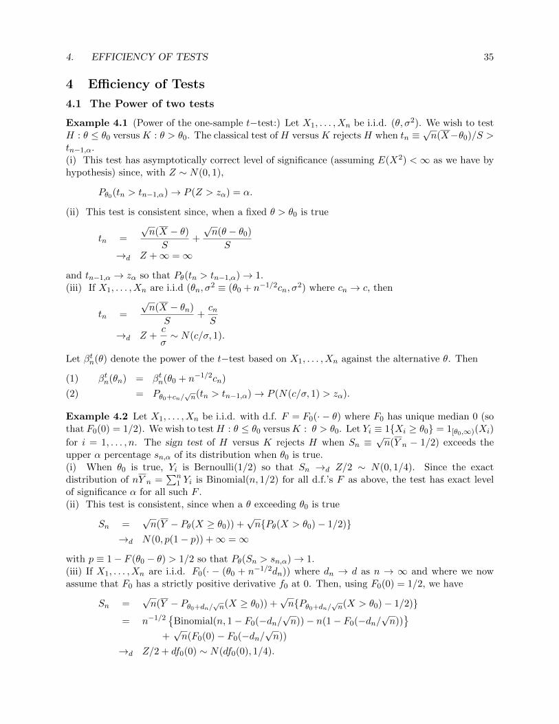
Example 4.1 (Power of the one-sample t−test:) Let X1, . . . , Xn be i.i.d. (θ, σ2). We wish to testH : θ ≤ θ0 versus K : θ > θ0. The classical test of H versus K rejects H when tn ≡
√n(X−θ0)/S >
tn−1,α.(i) This test has asymptotically correct level of significance (assuming E(X2) <∞ as we have byhypothesis) since, with Z ∼ N(0, 1),
Pθ0(tn > tn−1,α)→ P (Z > zα) = α.
(ii) This test is consistent since, when a fixed θ > θ0 is true
tn =
√n(X − θ)S
+
√n(θ − θ0)
S→d Z +∞ =∞
and tn−1,α → zα so that Pθ(tn > tn−1,α)→ 1.(iii) If X1, . . . , Xn are i.i.d (θn, σ
2 ≡ (θ0 + n−1/2cn, σ2) where cn → c, then
tn =
√n(X − θn)
S+cnS
→d Z +c
σ∼ N(c/σ, 1).
Let βtn(θ) denote the power of the t−test based on X1, . . . , Xn against the alternative θ. Then
βtn(θn) = βtn(θ0 + n−1/2cn)(1)
= Pθ0+cn/√n(tn > tn−1,α)→ P (N(c/σ, 1) > zα).(2)
Example 4.2 Let X1, . . . , Xn be i.i.d. with d.f. F = F0(· − θ) where F0 has unique median 0 (sothat F0(0) = 1/2). We wish to testH : θ ≤ θ0 versusK : θ > θ0. Let Yi ≡ 1{Xi ≥ θ0} = 1[θ0,∞)(Xi)
for i = 1, . . . , n. The sign test of H versus K rejects H when Sn ≡√n(Y n − 1/2) exceeds the
upper α percentage sn,α of its distribution when θ0 is true.(i) When θ0 is true, Yi is Bernoulli(1/2) so that Sn →d Z/2 ∼ N(0, 1/4). Since the exactdistribution of nY n =
∑n1 Yi is Binomial(n, 1/2) for all d.f.’s F as above, the test has exact level
of significance α for all such F .(ii) This test is consistent, since when a θ exceeding θ0 is true
Sn =√n(Y − Pθ(X ≥ θ0)) +
√n{Pθ(X > θ0)− 1/2)}
→d N(0, p(1− p)) +∞ =∞
with p ≡ 1− F (θ0 − θ) > 1/2 so that Pθ(Sn > sn,α)→ 1.(iii) If X1, . . . , Xn are i.i.d. F0(· − (θ0 + n−1/2dn)) where dn → d as n → ∞ and where we nowassume that F0 has a strictly positive derivative f0 at 0. Then, using F0(0) = 1/2, we have
Sn =√n(Y − Pθ0+dn/
√n(X ≥ θ0)) +
√n{Pθ0+dn/
√n(X > θ0)− 1/2)}
= n−1/2{
Binomial(n, 1− F0(−dn/√n))− n(1− F0(−dn/
√n))}
+√n(F0(0)− F0(−dn/
√n))
→d Z/2 + df0(0) ∼ N(df0(0), 1/4).
36 CHAPTER 6. TESTING
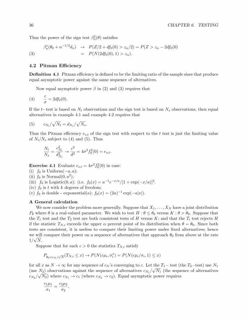
Thus the power of the sign test β2n(θ) satisfies
βsn(θ0 + n−1/2dn) → P (Z/2 + df0(0) > zα/2) = P (Z > zα − 2df0(0)
= P (N(2df0(0), 1) > zα).(3)
4.2 Pitman Efficiency
Definition 4.1 Pitman efficiency is defined to be the limiting ratio of the sample sizes that produceequal asymptotic power against the same sequence of alternatives.
Now equal asymptotic power β in (2) and (3) requires that
c
σ= 2df0(0).(4)
If the t−test is based on Nt observations and the sign test is based on Ns observations, then equalalternatives in example 4.1 and example 4.2 requires that
cNt/√Nt = dNs/
√Ns.(5)
Thus the Pitman efficiency es,t of the sign test with respect to the t test is just the limiting valueof Nt/Ns subject to (4) and (5). Thus
Nt
Ns=c2Nt
d2Ns
→ c2
d2= 4σ2f2
0 (0) = es,t.
Exercise 4.1 Evaluate es,t = 4σ2f20 (0) in case:
(i) f0 is Uniform(−a, a);(ii) f0 is Normal(0, a2);(iii) f0 is Logistic(0, a): (i.e. f0(x) = a−1e−x/a/[1 + exp(−x/a)]2.(iv) f0 is t with k degrees of freedom;(v) f0 is double - exponential(a); f0(x) = (2a)−1 exp(−a|x|).
A General calculation
We now consider the problem more generally. Suppose that X1, . . . , XN have a joint distributionPθ where θ is a real-valued parameter. We wish to test H : θ ≤ θ0 versus K : θ > θ0. Suppose thatthe T1 test and the T2 test are both consistent tests of H versus K; and that the Ti test rejects Hif the statistic TN,i exceeds the upper α percent point of its distribution when θ = θ0. Since bothtests are consistent, it is useless to compare their limiting power under fixed alternatives; hencewe will compare their power on a sequence of alternatives that approach θ0 from above at the rate1/√N .
Suppose that for each c > 0 the statistics TN,i satisfy
Pθ0+cN/√N (TN,i ≤ x)→ P (N(cµi, σ
xi ) = P (N(cµi/σi, 1) ≤ x)
for all x as N →∞ for any sequence of cN ’s converging to c. Let the T1− test (the T2−test) use N1
(use N2) observations against the sequence of alternatives cN1/√N1 (the sequence of alternatives
cN2/√N2) where cN1 → c1 (where cN2 → c2). Equal asymptotic power requires
c1µ1
σ1=c2µ2
σ2,

4. EFFICIENCY OF TESTS 37
and equal alternatives requires
cN1√N1
=cN2√N2
;
solving these simultaneously leads to
N2
N1=c2N2
c2N1
→ (µ1/σ1)2
(µ2/σ2)2= e1,2.(6)
Note that the efficiency e1,2 is independent of the common level of significance α of the tests, of theparticular value of the asymptotic power β, and of the particular sequences that converge to thevalues of c1 and c2 that are specified by the choice of β. Since so much is summarized in a singlenumber, the procedure is bound to have some shortcomings; however it can be extremely usefuland informative.
The quantity εi ≡ (µi/σi)2 is called the efficacy of the Ti−test, and hence the efficiency e1,2 is
the ratio of the efficacies.
Exercise 4.2 Define your idea of what the exact small sample efficiency es,t(α, β, n) of the sign testwith respect to the t−test should be. Compute some values of it in case X1, . . . , Xn are normal,and compare these values with the asymptotic value es,t = 2/π=.6366 . . . that was obtained inexercise 4.1.
Exercise 4.3 Now redefine Pitman efficiency to be the ratio of the squared distances from thealternative to the hypothesized valued θ0 that produce equal asymptotic power as equal samplesized approach infinity. Show that you get the same answer as before.
Note that if T1 and T2 are estimating the same thing (that is, if µ1 = µ2), then e1,2 is just theratio of the limiting variances.
Also note that the typical test of H : θ ≤ θ0 versus K : θ > θ0 is of the form: reject H if√n(T − Eθ0(T ))√V arθ0(
√n(T ))
> kn,α → zα.
Thus when θ0 + c/√n is true, intuitively we have (letting m(θ) ≡ Eθ(T ), and σ2
0 ≡ V arθ0(√nT )),
√n(T − Eθ0(T ))√V arθ0(
√n(T ))
=
√V arθ0+c/
√n(√n(T ))√
V arθ0(√n(T ))
√n(T − Eθ0+c/
√n(T ))√
V arθ0+c/√n(√n(T ))
+
√n(m(θ0 + c/
√n)−m(θ0)√
V arθ0(√n(T ))
→d 1 · Z +cm′(θ0)
σ0∼ N(cm′(θ0)/σ0, 1).
Thus we expect (m′(θ0)/σ0)2 to be the efficacy.
Exercise 4.4 Now consider testing H : θ = θ0 versus K : θ 6= θ0 on the basis of a two-sided testbased on either the T1 or the T2 statistics consider previously. Show that the same formula forPitman efficiency is appropriate for the two-side test also.
38 CHAPTER 6. TESTING
Exercise 4.5 Again consider testing H : θ = θ0 versus K : θ 6= θ0; but suppose now that
Tn,i →d χ2k(c
2δ2i ) as n→∞
under any sequence of alternatives θ0 + cn/√n having cn → c > 0 as n → ∞. Here k is a fixed
interger, and the limiting random variable has a noncentral chi-square distribution. Show that thePitman efficiency criterion leads to e1,2 = δ2
1/δ22 .
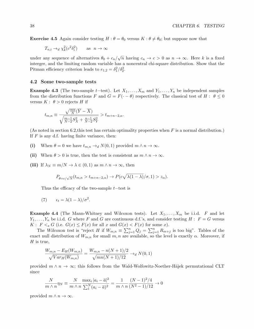
4.2 Some two-sample tests
Example 4.3 (The two-sample t−test). Let X1, . . . , Xm and Y1, . . . , Yn be independent samplesfrom the distribution functions F and G = F (· − θ) respectively. The classical test of H : θ ≤ 0versus K : θ > 0 rejects H if
tm,n ≡√
mnN (Y −X)√
m−1N−2S
2X + n−1
N−2S2Y
> tm+n−2,α.
(As noted in section 6.2,this test has certain optimality properties when F is a normal distribution.)If F is any d.f. having finite variance, then:
(i) When θ = 0 we have tm,n →d N(0, 1) provided m ∧ n→∞.
(ii) When θ > 0 is true, then the test is consistent as m ∧ n→∞.
(iii) If λN ≡ m/N → λ ∈ (0, 1) as m ∧ n→∞, then
Pθ=c/√N (tm,n > tm+n−2,α)→ P (c
√λ(1− λ)/σ, 1) > zα).
Thus the efficacy of the two-sample t−test is
εt = λ(1− λ)/σ2.(7)
Example 4.4 (The Mann-Whitney and Wilcoxon tests). Let X1, . . . , Xm be i.i.d. F and letY1, . . . , Yn be i.i.d. G where F and G are continuous d.f.’s, and consider testing H : F = G versusK : F <s G (i.e. G(x) ≤ F (x) for all x and G(x) < F (x) for some x).
The Wilcoxon test is “reject H if Wm,n ≡∑n
j=1Qj =∑n
j=1Rm+j is too big”. Tables of theexact null distribution of Wm,n for small m,n are available, so the level is exactly α. Moreover, ifH is true,
Wm,n − EH(Wm,n)√V arH(Wm,n)
=Wm,n − n(N + 1)/2√
mn(N + 1)/12→d N(0, 1)
provided m ∧ n → ∞; this follows from the Wald-Wolfowitz-Noether-Hajek permutational CLTsince
N
m ∧ nηN ≡
N
m ∧ nmaxi |ai − a|2∑N
1 (ai − a)2=
1
m ∧ n(N − 1)2/4
(N2 − 1)/12→ 0
provided m ∧ n→∞.

4. EFFICIENCY OF TESTS 39
The Mann-Whitney test is described as follows: let
Um,n ≡1
mn
m∑i=1
n∑j=1
1{Xi ≤ Yj}.
Mann and Whitney proposed to reject H if Um,n is “too big”. Since
mnUm,n + n(n+ 1)/2 = Wm,n,
when H is true we have
Um,n − 1/2√(N + 1)/12mn
→d N(0, 1) as m ∧ n→∞.
For arbitrary F and G
EUm,n = E1{X ≤ Y } = P (X ≤ Y ) =
∫FdG,
while, for arbitrary continuous F and G
V ar(√mnUm,n) = (n− 1)
∫(1−G)2dF
+ (m− 1)
∫F 2dG− (N − 1)
(∫FdG
)2
+
∫FdG
= (n− 1)V ar(1−G(X)) + (m− 1)V ar(F (Y )) +
∫FdG(1−
∫FdG).
We now consider the local alternatives Yd= X + c/
√N , or G = F (· − c/
√N). We also suppose
that λN = m/N → λ. Then
Um,n − 1/2√(N + 1)/12mn
=Um,n −
∫FdG√
(N + 1)/12mn+
∫FdG− 1/2√
(N + 1)/12mn
≡ Zm,n + am,n
where it seems intuitive that Zm,n →d Z ∼ N(0, 1) as N →∞ and
am,n =
√12mn
N(N + 1)
√N
{∫FdG− 1
2
}
=
√12mn
N(N + 1)
√N
{∫F (x)dF (x− c/
√N)−
∫FdF
}
=
√12mn
N(N + 1)
∫ √N(F (x− c/
√N)− F (x))dF (x)
→√
12λ(1− λ)c
∫f2(x)dx
assuming that F has density f with∫f2(x)dx <∞. Thus under (F,G) = (F, F (· − c/
√N))
Um,n − 1/2√(N + 1)/12mn
→d Z + c√
12λ(1− λ)
∫f2 ∼ N(c
√12λ(1− λ)
∫f2, 1).

40 CHAPTER 6. TESTING
Thus the efficacy of the U−test is
εU = 12λ(1− λ)
(∫f2(x)dx
)2
.(8)
Combining the efficacies in (7) and (8) for the t−test and the U−test respectively gives thePitman efficiency of the U−test with respect to the t−test:
eU,t(F ) =12λ(1− λ){
∫f2}2
λ(1− λ)/σ2= 12σ2
(∫f2
)2
.
Proposition 4.1 eU,t(F ) ≥ 108/125 = .864 . . ..
Proof. first note that eU,t(F ) = eU,t(F (·−a)/c). Thus it suffices to minimize∫f2(x)dx subject
to the restrictions∫x2f(x)dx = 1,
∫xf(x)dx = 0, f(x) ≥ 0,
∫f(x)dx = 1.
Consider minimizing
B(f) ≡∫ ∞−∞{f2(x) + f(x)2b(x2 − a2)}dx
with b > 0 subject to f ≥ 0 and∫f(x)dx = 0. Now
f2(x) + 2bf(x)(x2 − a2) = f(x){f(x) + 2b(x2 − a2)}= A{A+ 2b(x2 − a2) ≥ 0 for |x| ≥ a.
Thus take f(x) = 0 for |x| ≥ a and minimize the integrand pointwise for |x| ≤ a. This yieldsA ≡ f(x) = b(a2−x2). Thus the minimizer fa,b(x) ≡ f = b(a2−x2)1[−a,a](x). Choosing a and b so
that∫x2f(x)dx = 1 and
∫f(x) = 1 yields a =
√5, b = 3
√5/100, and hence
∫f2(x)dx = 3
√5/25.
Hence
eU,t ≥ 12{∫f2a,b(x)dx}2 = 12(9 · 5)/625 = 108/125.
2
Proof of asymptotic normality of Um,n under local alternatives Suppose that
XN,1, . . . , XN,m are i.i.d. FN
YN,1 . . . , YN,n are i.i.d. GN
where FN , GN , and H are continuous df’s satisfying ‖FN − H‖∞ → 0 and ‖GN − H‖∞ → 0as N → ∞. Let Fm and Gn denote the empirical df’s of XN,1 . . . , XN,m and YN,1, . . . , YN,mrespectively. Now
Um,n =
∫FmdGn.
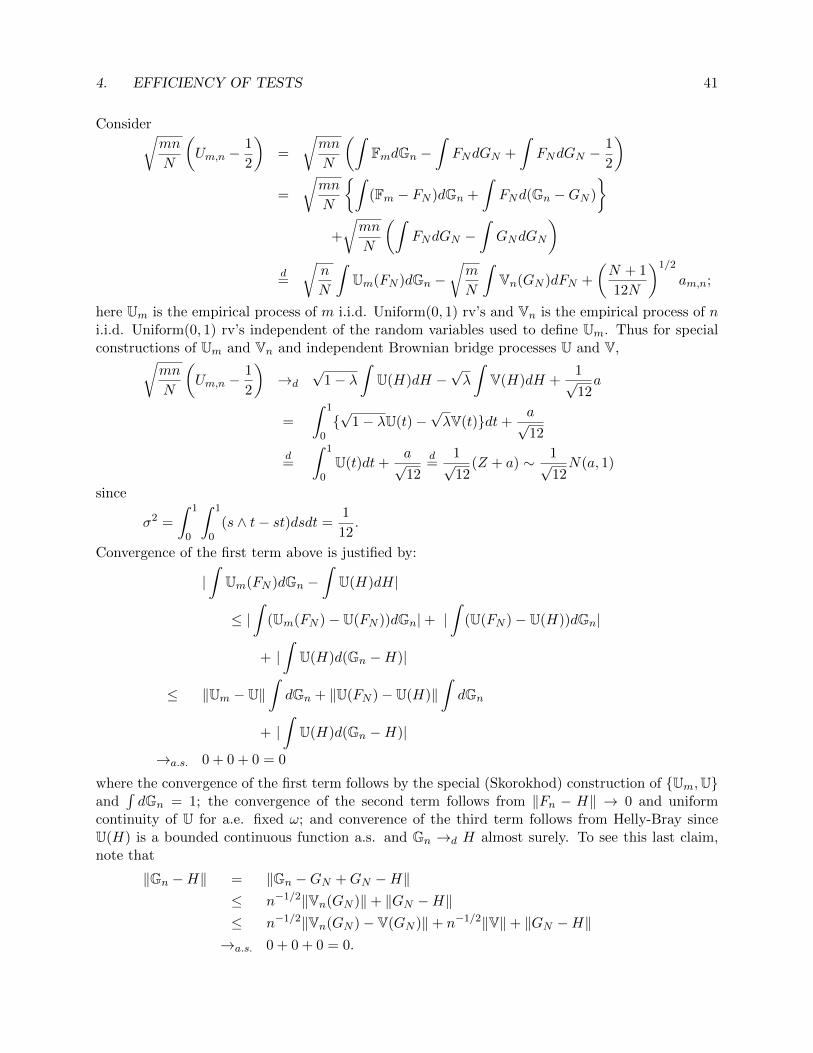
4. EFFICIENCY OF TESTS 41
Consider√mn
N
(Um,n −
1
2
)=
√mn
N
(∫FmdGn −
∫FNdGN +
∫FNdGN −
1
2
)=
√mn
N
{∫(Fm − FN )dGn +
∫FNd(Gn −GN )
}+
√mn
N
(∫FNdGN −
∫GNdGN
)d=
√n
N
∫Um(FN )dGn −
√m
N
∫Vn(GN )dFN +
(N + 1
12N
)1/2
am,n;
here Um is the empirical process of m i.i.d. Uniform(0, 1) rv’s and Vn is the empirical process of ni.i.d. Uniform(0, 1) rv’s independent of the random variables used to define Um. Thus for specialconstructions of Um and Vn and independent Brownian bridge processes U and V,√
mn
N
(Um,n −
1
2
)→d
√1− λ
∫U(H)dH −
√λ
∫V(H)dH +
1√12a
=
∫ 1
0{√
1− λU(t)−√λV(t)}dt+
a√12
d=
∫ 1
0U(t)dt+
a√12
d=
1√12
(Z + a) ∼ 1√12N(a, 1)
since
σ2 =
∫ 1
0
∫ 1
0(s ∧ t− st)dsdt =
1
12.
Convergence of the first term above is justified by:
|∫
Um(FN )dGn −∫
U(H)dH|
≤ |∫
(Um(FN )− U(FN ))dGn|+ |∫
(U(FN )− U(H))dGn|
+ |∫
U(H)d(Gn −H)|
≤ ‖Um − U‖∫dGn + ‖U(FN )− U(H)‖
∫dGn
+ |∫
U(H)d(Gn −H)|
→a.s. 0 + 0 + 0 = 0
where the convergence of the first term follows by the special (Skorokhod) construction of {Um,U}and
∫dGn = 1; the convergence of the second term follows from ‖Fn − H‖ → 0 and uniform
continuity of U for a.e. fixed ω; and converence of the third term follows from Helly-Bray sinceU(H) is a bounded continuous function a.s. and Gn →d H almost surely. To see this last claim,note that
‖Gn −H‖ = ‖Gn −GN +GN −H‖≤ n−1/2‖Vn(GN )‖+ ‖GN −H‖≤ n−1/2‖Vn(GN )− V(GN )‖+ n−1/2‖V‖+ ‖GN −H‖→a.s. 0 + 0 + 0 = 0.

42 CHAPTER 6. TESTING
Exercise 4.6 Evaluate eU,t(F ) = 12σ2(∫f2(x)dx)2 in case:
(i) f is Uniform[−a, a].
(ii) f is Normal.
(iii) f is Logistic.
(iv) f is tk.
(v) f is double-exponential.
Exercise 4.7 (General behavior of the centering constants for Um,n). Suppose that
‖√N(f
1/2N − h1/2)− 1
2αh1/2‖2 → 0, and ‖
√N(g
1/2N − h1/2)− 1
2βh1/2‖2 → 0.
Then
‖√N(FN −H)−
∫ ·−∞
αdH‖∞ → 0, and ‖√N(GN −H)−
∫ ·−∞
βdH‖∞ → 0.
Show that this implies (using∫αdH = 0 =
∫βdH) that
am,n →√
12λ(1− λ)
∫(1−H)(α− β)dH.
Check that the result for shift alternatives H ≡ F and G = F (· − c/√N) follows with α = 0 and
β = −f ′/f .
4.4 Pitman efficiency via Le Cam’s third lemma.
Often the limiting power and efficacy of a test can be easily derived via Le Cam’s third lemma,lemma 3.3.14. Recall tht the essence of that lemma is that the joint limiting distribution of astatistic and the local log-likelihood ratio under the null hypothesis determines the joint limitingdistribution of the statistic and the local log-likelhood ratio under the sequence of local alternatives.Here we simply illustrate this approach with the examples considered in section 6.4.1.
Example 4.5 The one-sample t−test again. Let X1, . . . , Xn be i.i.d. F = F0(· − θ) withθ = EF (X). Consider testing H : θ ≤ θ0 versus K : θ > θ0 using tn ≡
√n(X − θ0)/S. Suppose
that F0 has an absolutely continuous density f0 and that I0 ≡∫
(f ′0/f0)2f0dx < ∞. Let Ln ≡∏ni=1(fn/f)(Xi) where fn(x) = f0(x − θn), θn = θ0 + c/
√n, and f(x) = f0(x − θ0). Thus with
l(x) ≡ −(f ′/f)(x), under Pn = Pnf ,
logLn =c√n
n∑i=1
l(Xi)−c2
2I(f0) + op(1),
and, hence under Pn with pn(x) =∏ni=1 f(xi),(
tnlogLn
)→d N2
((0
−(c2/2)I(f0)
),
(1 σtLσtL c2I(f0)
))

4. EFFICIENCY OF TESTS 43
where
σtL = eEfX − θ0
σl(X) = cEf0
{−f′0(X)
f0(X)
}.
But
1 =θn − θ0
c/√n
=1
c/√n{Efn(X)− Ef (X)} = Ef
{X
((fn/f)(X)− 1
c/√n
)},
where the right side converges to Ef{X(−f ′/f)(X)}. Thus 1 = Ef{X(−f ′/f)(X)} and σtL = c/σ.Hence it follows from Le Cam’s third lemma with qn(x) =
∏ni=1 fn(xi) that, under Qn,(
tnlogLn
)→d N2
((c/σ
+(c2/2)I(f0)
),
(1 σtLσtL c2I(f0)
)).
Hence the efficacy of the t−test is (again) εt = 1/σ2.
Example 4.6 The one-sample sign test again. Now consider the sign statistic Sn =√n(Y −
1/2) where Yi ≡ 1(θ0,∞)(Xi) and Ln is as above. Then under Pn with pn(x) =∏ni=1 f(xi),(
SnlogLn
)→d N2
((0
+(c2/2)I(f0)
),
(1 σSLσSL c2I(f0)
))where
σSL ≡ cEf1(θ0,∞)(X)l(X) = −c∫ ∞θ0
f ′
f(x)f(x)dx = cf(θ0).
Hence, by Le Cam’s third lemma(Sn
logLn
)→d N2
((cf(θ0)
+(c2/2)I(f0)
),
(1 cf(θ0)
cf(θ0) c2I(f0)
))and it follows that the efficacy of the sign test is εS = 4f2(θ0) = 4f2
0 (0). Combining the two efficaciesεt and εS yields the Pitman efficiency of the sign test relative to the t−test, eS,t = 4σ2f2
0 (0).

44 CHAPTER 6. TESTING
5 Confidence Sets and p−values
The theory of testing that has been developed in the previous sections in this chapter connectswith with estimation theory via the construction of confidence sets. The material outlined in thissection is drawn in large part from Sections 3.5 (pages 72-77) and 5.4 (pages 161-162) of Lehmannand Romano (2005), and Section 5.8 (pages 257 - 264) of Ferguson (1967).
First, a definition:
Definition 5.1 Let {S(x)} ≡ {S(x) : x ∈ X} be a family of subsets of the parameter space Θ fora given sample space X . Then {S(x)} is said to be a family of confidence sets of confidence level1− α if
Pθ(S(X) contains θ) = Pθ(θ ∈ S(X)) = 1− α.
Construction of confidence sets from tests: Let A(θ0) denotes the acceptance region of a sizeα nonrandomized test ϕ of the hypothesis H0 : θ = θ0 against any alternative. That is
ϕ(x) =
{1 if x /∈ A(θ0)0 if x ∈ A(θ0)
where Pθ0(X ∈ A(θ0)) = 1−α. If we consider the sets A(θ), θ ∈ Θ, we have a family of acceptanceregions, each a subset of X such that
Pθ(X ∈ A(θ)) = 1− α.
Define S(x) = {θ : x ∈ A(θ)}, so that {θ ∈ S(X)} = {X ∈ A(θ)}. Then it follows that
Pθ(θ ∈ S(X)) = Pθ(X ∈ A(θ)) = 1− α,
so the resulting family {S(x) : x ∈ X} is a family of confidence sets of level 1− α.
Here are three examples:
Example 5.1 Suppose that X ∼ N(µ, 1), and consider testing H : µ = µ0 versus K : µ > µ0.By the Karlin - Rubin theorem, the UMP test is ϕ(X) = 1{X > µ0 + zα} with acceptance regionA(µ0) = {x : x ≤ µ0 + zα}. Thus
A(µ) = {x : x ≤ µ+ zα},S(x) = {µ : µ ≥ x− zα}.
Thus it follows that
1− α = Pµ(X ≤ µ+ zα) = Pµ(µ ≥ X − zα)
= Pµ(µ ≥ µα(X)) with µα(X) ≡ X − zα= Pµ(µ ∈ [µα(X),∞)) = Pµ(µ ∈ S(X))
where S(X) ≡ [µα(X),∞) = [X − zα,∞), and hence the family S(X) is a family of 1 − α levelconfidence sets for µ.

5. CONFIDENCE SETS AND P−VALUES 45
Example 5.2 Suppose that X1, . . . , Xn are i.i.d. with continuous distribution function F on [0, 1].Consider testing H : F = F0 (continuous) versus K : F <s F0 (i.e. F (x) ≥ F0(x) with strictinequality for some x). One natural test statistic is
Rn ≡ sup0<x≤1
Fn(x)
F0(x).
Now by Theorem 2.3.1 (and the discussion in Section 2.4) Fnd= Gn(F0) where Gn is the empirical
distribution function of i.i.d. Uniform(0, 1) random variables ξ1, . . . , ξn. Therefore
PF0(Rn > r) = PF0
(sup
0<x≤1
Gn(F0(x))
F0(x)> r
)= P
(sup
0<u<1
Gn(u)
u> r
)= 1/r, for r ≥ 1;
this is a result due to Daniels (1945); see e.g. Shorack and Wellner (1986), Theorem 9.1.2, page345 . Thus the test
ϕ(X) =
{1, if Rn > 1/α0, if Rn ≤ 1/α,
is a size α test with acceptance region
A(F0) =
{X : sup
0<x≤1
Fn(x)
F0(x)≤ 1/α
}= {X : αFn(x) ≤ F0(x) for all 0 < x ≤ 1} ,
A(F ) = {X : αFn(x) ≤ F (x) for all 0 < x ≤ 1} ,S(X) = {F : F (x) ≥ αFn(x) for all 0 < x ≤ 1}.
Thus
PF {F ∈ S(X)} = PF (F : F (x) ≥ αFn(x) for all 0 < x ≤ 1)
= PF
(sup
0<x≤1
Fn(x)
F (x)≤ 1/α
)= 1− α.
Example 5.3 Suppose that X1, . . . , Xn are i.i.d. Weibull (α, β) as in Example 3.x.y. Considertesting H : (α, β) = (α0, β0) versus K : (α, β) 6= (α0, β0). From the theory developed in Chapter4 we know that the likelihood ratio test based on the statistic
λn ≡ λn(α0, β0) ≡supα>0,β>0 Ln(α, β)
Ln(α0, β0)
satisfies
2 log λn(α0, β0)→d χ22
when α0, β0 are true. Therefore the acceptance sets
An(α0, β0) = {X : 2 log λn(α0, β0) ≤ χ22,δ}

46 CHAPTER 6. TESTING
where P (χ22 > χ2
2,δ) = δ satisfy
Pα0,β0(An(α0, β0))→ 1− δ, as n→∞,
and, similarly,
Pα,β(An(α, β))→ 1− δ, as n→∞.
But then
Pα,β(An(α, β)) = Pα,β((α, β) ∈ Sn(X))→ 1− δ
for the associated confidence sets
Sn(X) = {(α, β) ∈ R+2 : 2 log λn(α, β) ≤ χ22,δ}.
How should we choose a family of confidence sets? One natural criterion is to minimize theprobability of covering false values. That is, we should try to make
Pθ′(θ ∈ S(X))
small if θ 6= θ′. It turns out that optimality properties of tests carry over or translate into optimalityproperties of confidence sets. One version of this is given in the following theorem.
Theorem 5.1 Let A(θ0) be the acceptance region of a UMP test of size α of the hypothesisH0 : θ = θ0 versus H1 : θ ∈ Θ1. Then {S(x)} defined by
{θ ∈ S(x)} = {x ∈ A(θ)}
minimizes Pθ′(θ ∈ S(X)) for all θ′ ∈ Θ1 among all level 1− α families of confidence sets.
See e.g. Lehmann and Romano (2005), pages 72 - 77 and 164 - 168.Suppose that θ = (ν, ξ) ∈ Θ, ν ∈ R, ξ ∈ Rk for some k. A lower confidence bound for ν is a
function ν(x) such thatPν,ξ(ν(X) ≤ ν) ≥ 1− α for all ν, ξ.
Similarly, a confidence interval for ν at confidence level 1− α is given by ν(x), ν(x) satisfying
Pν,ξ(ν(X) ≤ ν ≤ νX)) ≥ 1− α for all ν, ξ.
Connection with estimation: If ν(X) satisfies
Pν,ξ(ν(X) ≤ ν) = Pν,ξ(ν(X) ≥ ν) = 1/2,
then ν(X) is a median unbiased estimator of ν. For the use of this in developing “R-estimators oflocation”, see e.g. Hodges and Lehmann (1963).
p-values:See Lehmann and Romano, pages 57, 63-65, 97-98, 108-109, and 139.Consider a family of tests ϕα(X) = 1Acα(X) of H versus K with rejection regions Acα satisfying
Acα ⊂ Acα′ if α < α′.(1)
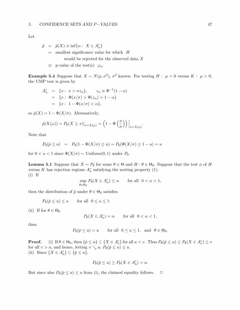
5. CONFIDENCE SETS AND P−VALUES 47
Let
p = p(X) ≡ inf{α : X ∈ Acα}= smallest significance value for which H
would be rejected for the observed data X
≡ p-value of the test(s) ϕα.
Example 5.4 Suppose that X ∼ N(µ, σ2), σ2 known. For testing H : µ = 0 versus K : µ > 0,the UMP test is given by
Acα = {x : x > σzα}, zα ≡ Φ−1(1− α)
= {x : Φ(x/σ) > Φ(zα) = 1− α}= {x : 1− Φ(x/σ) < α},
so p(X) = 1− Φ(X/σ). Alternatively,
p(X(ω)) = P0(X ≥ x)|x=X(ω) =(
1− Φ(xσ
)) ∣∣∣x=X(ω)
.
Note that
P0(p ≤ u) = P0(1− Φ(X/σ) ≤ u) = P0(Φ(X/σ) ≥ 1− u) = u
for 0 < u < 1 since Φ(X/σ) ∼ Uniform(0, 1) under P0.
Lemma 5.1 Suppose that X ∼ Pθ for some θ ∈ Θ and H : θ ∈ Θ0. Suppose that the test φ of Hversus K has rejection regions Acα satisfying the nesting property (1).(i) If
supθ∈Θ0
Pθ(X ∈ Acα) ≤ α for all 0 < α < 1,
then the distribution of p under θ ∈ Θ0 satisfies
Pθ(p ≤ u) ≤ u for all 0 ≤ u ≤ 1.
(ii) If for θ ∈ Θ0
Pθ(X ∈ Acα) = α for all 0 < α < 1,
then
Pθ(p ≤ u) = u for all 0 ≤ u ≤ 1, and θ ∈ Θ0.
Proof. (i) If θ ∈ Θ0, then {p ≤ u} ⊂ {X ∈ Acv} for all u < v. Thus Pθ(p ≤ u) ≤ Pθ(X ∈ Acv) ≤ vfor all v > u, and hence, letting v ↘ u, Pθ(p ≤ u) ≤ u.(ii) Since {X ∈ Acu} ⊂ {p ≤ u},
Pθ(p ≤ u) ≥ Pθ(X ∈ Acu) = u.
But since also Pθ(p ≤ u) ≤ u from (i), the claimed equality follows. 2

48 CHAPTER 6. TESTING
Example 5.5 (Test for µ when X ∼ N(µ, σ2), continued.) What is the distribution of p underµ > 0?
Pµ(p ≤ u) = Pµ(1− Φ(X/σ) ≤ u) = Pµ(X ≥ σΦ−1(1− u))
= Pµ
(X − µσ
≥ Φ−1(1− u)− µ
σ
)= 1− Φ(Φ−1(1− u)− µ/σ).
Note that sinceΦ−1(1− u)− µ/σ ≤ Φ−1(1− u),
it follows thatΦ(Φ−1(1− u)− µ/σ) ≤ 1− u,
and hencePµ(p ≤ u) = 1− Φ(Φ−1(1− u)− µ/σ) ≥ 1− (1− u) = u.