Extending the Johnson-Neyman Procedure to Categorical

Independent Variables: Mathematical Derivations and

Computational Tools

A Thesis

Presented in Partial Fulfillment of the Requirements for the DegreeMaster of Arts in the Graduate School of The Ohio State University

By

Amanda Kay Montoya, B.S.

Graduate Program in Psychology

The Ohio State University

2016

Master’s Examination Committee:

Andrew F. Hayes, Advisor

Michael C. Edwards

Duane T. Wegener

c© Copyright by

Amanda Kay Montoya

2016

Abstract

Moderation analysis is used throughout many scientific fields, including psychol-

ogy and other social sciences, to model contingencies in the relationship between some

independent variable (X) and some outcome variable (Y ) as a function of some other

variable, typically called a moderator (M). Inferential methods for testing moderation

provide only a simple yes/no decision about whether the relationship is contingent.

These contingencies can often be complicated. Researcher often need to look closer.

Probing the relationship between X and Y at different values of the moderator pro-

vides the researcher with a better understanding of how the relationship changes

across the moderator. There are two popular methods for probing an interaction:

simple slopes analysis and the Johnson-Neyman procedure. The Johnson-Neyman

procedure is used to identify the point(s) along a continuous moderator where the

relationship between the independent variable and the outcome variable transition(s)

between being statistically significant to nonsignificant or vice versa. Implementation

of the Johnson-Neyman procedure when X is either dichotomous of continuous is

well described in the literature; however, when X is a multicategorical variable it is

not clear how to implement this method. I begin with a review of moderation and

popular probing techniques for dichotomous and continuous X. Next, I derive the

Johnson-Neyman solutions for three groups and continue with a partial derivation

for four groups. Solutions for the four-group derivation rely on finding the roots of

ii

an eighth-degree polynomial for which there is no algebraic solution. I provide an

iterative computer program for SPSS and SAS that solves for the Johnson-Neyman

boundaries for any number of groups. I describe the performance of this program,

relative to known solutions, and typical run-times under a variety of circumstances.

Using a real dataset, I show how to analyze data using the tool and how to interpret

the results. I conclude with some consideration about when to use and when not to

use this tool, future directions, and general conclusions.

iii

This thesis is dedicated to my friends and family who have supported me in all my

various dreams. Particularly to my mother Lori for always seeing the best in me

and my best friend Colleen for being a rock and support through the toughest times

in life. Even though we are far apart you are always close to my heart.

iv

Acknowledgments

I would like to thank my committee members for their detailed feedback and

questions, particularly my advisor Dr. Hayes for suggesting this topic and guiding me

through the research process. I would like to thank the attendees of the Quantitative

Psychology Graduate Student Meeting for their helpful feedback, particularly in the

early stages of development. Special thanks to J. R. R. Tolkien for inspiring the name

of the tool.

v

Vita

May 8, 1991 . . . . . . . . . . . . . . . . . . . . . . . . . . . . . . . . BornSeattle, WA

2011 . . . . . . . . . . . . . . . . . . . . . . . . . . . . . . . . . . . . . . . .A.A. Psychology,North Seattle Community College

2013 . . . . . . . . . . . . . . . . . . . . . . . . . . . . . . . . . . . . . . . .B.S. PsychologyUniversity of Washington

2014-present . . . . . . . . . . . . . . . . . . . . . . . . . . . . . . . .Graduate Fellow,Holstein University.

Fields of Study

Major Field: Psychology

vi

Table of Contents

Page

Abstract . . . . . . . . . . . . . . . . . . . . . . . . . . . . . . . . . . . . . . . ii

Dedication . . . . . . . . . . . . . . . . . . . . . . . . . . . . . . . . . . . . . . iv

Acknowledgments . . . . . . . . . . . . . . . . . . . . . . . . . . . . . . . . . . v

Vita . . . . . . . . . . . . . . . . . . . . . . . . . . . . . . . . . . . . . . . . . vi

List of Tables . . . . . . . . . . . . . . . . . . . . . . . . . . . . . . . . . . . . x

List of Figures . . . . . . . . . . . . . . . . . . . . . . . . . . . . . . . . . . . xi

1. Introduction . . . . . . . . . . . . . . . . . . . . . . . . . . . . . . . . . . 1

2. Linear Moderation Analysis in OLS Regression . . . . . . . . . . . . . . 5

2.1 Inference about Moderation . . . . . . . . . . . . . . . . . . . . . . 52.2 Probing Moderation Effects . . . . . . . . . . . . . . . . . . . . . . 10

2.2.1 Simple-Slopes Analysis . . . . . . . . . . . . . . . . . . . . . 102.2.2 The Johnson-Neyman Procedure . . . . . . . . . . . . . . . 132.2.3 Tools for Probing . . . . . . . . . . . . . . . . . . . . . . . . 18

3. Moderation of the Effect of a Categorical Variable . . . . . . . . . . . . . 20

3.1 Inference about Moderation . . . . . . . . . . . . . . . . . . . . . . 213.2 Probing Moderation Effects . . . . . . . . . . . . . . . . . . . . . . 23

3.2.1 Simple-Slopes Analysis . . . . . . . . . . . . . . . . . . . . . 24

vii

4. Derivations of the Johnson-Neyman Procedure for Multiple Groups . . . 28

4.1 Three Groups . . . . . . . . . . . . . . . . . . . . . . . . . . . . . . 294.2 Four Groups . . . . . . . . . . . . . . . . . . . . . . . . . . . . . . 35

5. OGRS: An Iterative Tool for Finding Johnson-Neyman Regions of Signif-icance for Omnibus Group Differences . . . . . . . . . . . . . . . . . . . 40

5.1 Program Inputs . . . . . . . . . . . . . . . . . . . . . . . . . . . . . 405.1.1 Required Inputs . . . . . . . . . . . . . . . . . . . . . . . . 415.1.2 Optional Inputs . . . . . . . . . . . . . . . . . . . . . . . . . 415.1.3 Command Line Example . . . . . . . . . . . . . . . . . . . . 44

5.2 Internal Processes . . . . . . . . . . . . . . . . . . . . . . . . . . . 455.2.1 Regression Results . . . . . . . . . . . . . . . . . . . . . . . 455.2.2 Finding Johnson-Neyman Solutions . . . . . . . . . . . . . . 46

5.3 Program Outputs . . . . . . . . . . . . . . . . . . . . . . . . . . . . 505.4 Programming Decisions . . . . . . . . . . . . . . . . . . . . . . . . 515.5 Program Performance . . . . . . . . . . . . . . . . . . . . . . . . . 53

5.5.1 Accuracy . . . . . . . . . . . . . . . . . . . . . . . . . . . . 535.5.2 Run Time . . . . . . . . . . . . . . . . . . . . . . . . . . . . 56

6. Party Differences in Support of Government Action to Mitigate ClimateChange . . . . . . . . . . . . . . . . . . . . . . . . . . . . . . . . . . . . 64

7. Discussion . . . . . . . . . . . . . . . . . . . . . . . . . . . . . . . . . . . 72

7.1 Uses and Non-Uses . . . . . . . . . . . . . . . . . . . . . . . . . . . 737.2 Future Directions . . . . . . . . . . . . . . . . . . . . . . . . . . . . 737.3 Conclusion . . . . . . . . . . . . . . . . . . . . . . . . . . . . . . . 76

References . . . . . . . . . . . . . . . . . . . . . . . . . . . . . . . . . . . . . . 78

Appendices

A. OGRS Macro for SPSS . . . . . . . . . . . . . . . . . . . . . . . . . . . . 82

B. OGRS Macro Documentation for SPSS . . . . . . . . . . . . . . . . . . . 90

B.1 Overview . . . . . . . . . . . . . . . . . . . . . . . . . . . . . . . . 90

viii

B.2 Preparation for Use . . . . . . . . . . . . . . . . . . . . . . . . . . 91B.3 Model Specification . . . . . . . . . . . . . . . . . . . . . . . . . . . 91B.4 Confidence Level . . . . . . . . . . . . . . . . . . . . . . . . . . . . 92B.5 Convergence Criteria . . . . . . . . . . . . . . . . . . . . . . . . . . 93B.6 Initial Iterations . . . . . . . . . . . . . . . . . . . . . . . . . . . . 93B.7 Decimals . . . . . . . . . . . . . . . . . . . . . . . . . . . . . . . . 93

C. OGRS Macro for SAS . . . . . . . . . . . . . . . . . . . . . . . . . . . . 95

D. OGRS Macro Documentation for SAS . . . . . . . . . . . . . . . . . . . 102

D.1 Overview . . . . . . . . . . . . . . . . . . . . . . . . . . . . . . . . 102D.2 Preparation for Use . . . . . . . . . . . . . . . . . . . . . . . . . . 103D.3 Model Specification . . . . . . . . . . . . . . . . . . . . . . . . . . . 103D.4 Confidence Level . . . . . . . . . . . . . . . . . . . . . . . . . . . . 104D.5 Convergence Criteria . . . . . . . . . . . . . . . . . . . . . . . . . . 105D.6 Initial Iterations . . . . . . . . . . . . . . . . . . . . . . . . . . . . 105D.7 Decimals . . . . . . . . . . . . . . . . . . . . . . . . . . . . . . . . 106

ix

List of Tables

Table Page

5.1 Accuracy of OGRS Johnson-Neyman Solutions for SPSS and SAS . . 57

5.2 Run Time in Seconds for OGRS with Three Groups . . . . . . . . . . 61

5.3 Run Time in Seconds for OGRS with Five Groups . . . . . . . . . . . 62

5.4 Run Time in Seconds for OGRS with Seven Groups . . . . . . . . . . 63

x

List of Figures

Figure Page

6.1 OGRS Output for SPSS: Global Data . . . . . . . . . . . . . . . . . . 67

6.2 OGRS Output for SAS: Global Data . . . . . . . . . . . . . . . . . . 68

6.3 Graph of Predicted Support for Government Action across Party Iden-tification and Age . . . . . . . . . . . . . . . . . . . . . . . . . . . . . 69

xi

Chapter 1: Introduction

When a researcher believes that the relationship between an independent variable

(X) and an outcome (Y ) may depend on some other variable (M) they can test this

hypotheses by allowing for moderation of the effect of X on Y by M in a regression

analysis. For example, Kim and Baek (2014) were interested in if people’s selec-

tive self-presentation online (X ) predicted their online life satisfaction (Y ), and if

this relationship depended on self-esteem (M ). Indeed, they found that selective self-

presentation online predicted increased online life satisfaction, and this relationship

was larger among those with low self-esteem than those with high self-esteem. Siy and

Cheryan (2013) studied how Asian Americans reacted to positive stereotypes based

on their Asian culture. They found that those who had an independent self-construal

(M ) as compared to an interdependent self-construal, reactived more negatively (Y )

when they were positively stereotyped (X ). In this study self-construal, the modera-

tor, was measured on a single scale which ranged from interdependent to independent.

Research often begins with a simple correlation question: “Does this relate to

that?”. As a research area develops, these questions may gain some nuance, such as

whether or not two things are always related in the same way, or does the relation-

ship depend on other variables. Questions about contingencies help define boundary

1

conditions for the relationships between variables. These types of analysis can pro-

vide explanations for seemingly contradictory results. For example, Campbell (1990)

found that boys had more positive attitudes towards computers than girls. However,

DeRemer (1989) found that girls had more positive attitudes toward computers than

boys. One major difference between these two studies is the age of students sampled.

Campbell (1990) looked at high school students and DeRemer (1989) examined stu-

dents in grades three and six. A single study which sampled students from a variety of

grades could show that the relationship between gender and computer attitudes varies

with age or school grade, as was shown in a meta-analysis by Whitley Jr. (1997).

Researchers throughout psychology are often interested in moderators such as sit-

uational variables, individual differences, and experimental conditions. Using mod-

eration analysis allows researchers to more clearly understand under what conditions

certain effects occur or do not occur, how their magnitude varies, and how their direc-

tion can change. Moderation analyses are important not only for improving theory,

but also for improving practical applications. For example, given the results of a

moderation analysis, it has been suggested that practitioners can assign individuals

to treatments, such as educational classes, where they are predicted to have the most

beneficial outcomes given their scores on the moderator (Forster, 1971).

Statistical moderation analysis has been used in psychology for many years and is

taught in introductory regression classes to most graduate students in the field. Many

books have been written on the topic of moderation and interactions (e.g., Jaccard

& Turrisi, 2003; Aiken & West, 1991) and complete chapters and full sections of

introductory regression and statistics books are dedicated to this topic (e.g., Cohen,

Cohen, West, & Aiken, 2003; Field, 2013; Darlington & Hayes, 2017; Hayes, 2013;

2

Howell, 2007). Researchers also often use statistical methods to probe interactions

to better understand the nature of the contingent effect they are interested in. By

expanding methods for probing interactions this thesis provides additional tools for

psychology researchers to answer the questions they are interested in.

The aim of this thesis is to provide a tool to help researchers probe moderated rela-

tionships when the independent variable of interest is categorical, particularly having

three or more categories, using the Johnson-Neyman procedure. Moderation analysis

involves both inferential methods for decisions of moderation or no moderation and

probing methods for investigating the nature of the moderated relationship. The topic

of moderation with categorical independent variables has been discussed in a variety

of books and publications (e.g., Cohen et al., 2003; Huitema, 1980; Spiller, Fitzimons,

Lynch Jr., & McClelland, 2013); however, probing methods for categorical predictors

are less frequently discussed. Common probing methods for examining moderated

relationships include two approaches: the simple slopes approach and the Johnson-

Neyman procedure. Some researchers have discussed how to apply the simple slopes

approach for moderated relationships with categorical independent variables and ei-

ther dichotomous or continuous moderators (Hayes, 2013; Spiller et al., 2013). The

primary contribution of this thesis is to describe how the the Johnson-Neyman pro-

cedure can be generalized to situations where the independent variable is categorical

and the moderator is continuous. This case is particularly of interest to researchers

focused on the effect of the independent variable on the outcome at different values of

the moderator, rather than an estimate of the effect of the moderator on the outcome

at each level of the independent variable.

3

I begin with an overview of the procedures for testing moderation as well as the two

methods for probing moderated relationships: simple slopes analysis and the Johnson-

Neyman procedure. I will focus on a model comparison approach, using ordinary least

squares (OLS) for model estimation. I will then give a brief discussion of the historical

development of the Johnson-Neyman procedure. I continue by describing how to

estimate competing models in order to test moderation hypotheses with categorical

independent variables and implementation of the simple slopes method in these cases.

I then provide an analytical derivation of the Johnson-Neyman procedure with a 3-

group categorical variable and then start the derivation for a 4-group categorical

variable. As the number of groups (k) increases, the Johnson-Neyman procedure

relies on finding the roots of a 2k−1 degree polynomial. By the Abel-Ruffini theorem,

there are no general algebraic solutions for polynomial equations of degree five or

higher (Abel, 1824; Ruffini, 1799), meaning Johnson-Neyman solutions do not have

closed forms and cannot be found using traditional methods. I propose an iterative

computational method which finds the Johnson-Neyman solutions, and will provide

a tool, OGRS, to make this analysis easy to do using SPSS or SAS. I will illustrate

how to use this tool and interpret the results using two examples of real data from

psychology.

4

Chapter 2: Linear Moderation Analysis in OLS Regression

Moderation analysis using ordinary least squares regression (OLS) has two major

parts. First, a researchers tests if there is sufficient evidence that the relationship

between the independent variable and the outcome depends on some moderator. If

evidence of moderation in found, researchers often probe the interaction in order to

better understand and visualize the contingent relationship. This practice is much

like the practice of examining simple effects in ANOVA. In this chapter I describe

common methods for both inference about moderation and probing interactions in

linear moderation analysis using OLS regression.

2.1 Inference about Moderation

Though moderation can be tested in a variety of ways, the focus of this paper

will be using OLS regression for model estimation. Linear moderation is traditionally

tested by estimating and comparing the fit of two models, one with no contingent

relationships and one which allows for contingent relationships.

Model 1: Yi = b∗0 + b∗1Xi + b∗2Mi + ε∗i where εiiid∼ N(0, σ∗2)

Model 2: Yi = b0 + ΘX→Y |MXi + b2Mi + εi where εiiid∼ N(0, σ2)

ΘX→Y |M = b1 + b3Mi

5

In Models 1 and 2, Y is a continuous outcome variable which is being predicted.

The predictor variables in the models are X and M ’s. Within the context of modera-

tion, it is often helpful to frame the problem with respect to an independent variable,

the variable whose effect on Y is of interest, and a moderator, the variable which

is believed to influence the independent variable’s effect on Y . I will use X as the

independent variable and M as the moderator variable throughout. In Model 1, b∗0,

b∗1, and b∗2, are the population regression coefficients. In Model 2, b0, b1, b2, and b3

are the population regression coefficients. The stars in Model 1 are meant to indicate

that the coefficients are different from the coefficients in Model 2. In Model 1 the

effect of X on Y is not contingent on M but, rather, is constant, b∗1. In Model 2

however, the effect of X on Y is ΘX→Y |M , the conditional effect of X on Y at some

value of M , which is defined as a linear function of M . In this way, X’s effect on Y

depends on M , and is allowing for a certain type of moderation, linear moderation.

The effect ΘX→Y |M could be any defined function of M , such as a quadratic function,

but because linear moderation is most common in psychology, this thesis will focus

solely on linear moderation. Also note that the error terms in these equations are

assumed to be normally distributed with a constant variance σ2 or σ∗2. This will be

the case throughout this thesis but to avoid needless repetition this notation will be

omitted in future equations.

Model 1 is nested within Model 2. Specifically, if the b3 parameter is zero in

the population, then Model 2 simplifies to Model 1. This can be shown by plugging

ΘX→Y |M into the equation for Model 2 and expanding terms:

Yi = b0 + b1Xi + b2Mi + b3XiMi + εi

6

By setting b3 = 0:

Yi = b0 + b1Xi + b2Mi + 0XiMi + εi

Yi = b0 + b1Xi + b2Mi + εi

This last model is the equivalent to Model 1. This shows how Model 1 is nested

within Model 2.

The most common way to test for linear moderation in this case is to test if b3

is significantly different from zero in Model 2. If this coefficient is not significantly

different from zero, there is insufficient evidence that allowing the effect of X on Y

to depend on M improves the fit of the model, and so it is more reasonable to say

this relationship is not contingent.

An equivalent way to test for linear moderation is to use hierarchical OLS regres-

sion. Though this method may seem excessively complicated as compared to testing

one coefficient, this method generalizes to the case of a categorical X whereas the

test of b3 does not. Because of this, I will focus on hierarchical OLS as the method

of inference for moderation effects. A researcher would first estimate Model 1 then

add the product term, XiMi, to estimate Model 2. Comparing these two models will

test if allowing the relationship between X and Y to be contingent on M explains

additional variance in the outcome variable. This type of analysis can be completed

using any number of statistical packages. An F statistic corresponding to the change

in the variance explained can be calculated using Equation 2.1.

F =df2(R2

2 −R21)

q(1−R22)

(2.1)

Here the subscript on the R2 and df refer to the model number: Models 1 and

2 respectively as described above. The residual degrees of freedom in Model 2 is

7

noted by df2. The variance explained in Y in Model 1 and Model 2, are R21 and R2

2

respectively, and q is the number of constraints made to Model 2 to get Model 1. In

the situation where X is dichotomous or continuous, q is always 1, but as we move

into the case of a categorical X, q will depend on the number of categories in X. This

F -value is then compared to a critical F to decide if it is significant or the cumulative

distribution function is used to calculate the area to the right of the observed F -value

to calculate a p-value, the probability of observing this change in R2 assuming that

the relationship between X and Y is linearly independent of M (i.e. not contingent).

An inference about whether the relationship between X and Y is dependent on

M is important, but this inference does not completely describe the nature of the

contingency. The relationship between X and Y may get stronger or weaker as M

increases, and in order to understand the full nature of the contingency, it is impor-

tant to interpret the sign and magnitude of the regression coefficients. In multiple

regression without interactions, the regression coefficients are an estimate of the ef-

fect of each variable controlling for the other variables or holding the other variables

constant. For example, in Model 1 an estimate of b∗1 would be interpreted as the

expected change in Y for a one unit change in X, holding M constant.

In regression models with interactions, the interpretations of the coefficients are

no longer estimates of effects controlling for the other variables, but rather they are

conditional effects. The estimate of the coefficient b0 has the same interpretation as b∗0:

the expected value of Y when both X and M are zero. The other coefficients, however,

do not correspond with their counterparts in Model 1. They cannot be interpreted

as holding the other variables constant, because a one unit change in X would also

result in a change in XM when M is nonzero. In the model with interactions, b1

8

can be interpreted as the expected change in Y with a one unit change in X when

M is zero. Similarly, b2 can be interpreted as the expected change in Y with a one

unit change in M when X is zero. These two effects, b1 and b2, are conditioned on

certain variables being zero. The b3 parameter can be best understood by examining

the equation for ΘX→Y |M . From this equation it is clear that and estimate of b3 is

the expected change in the effect of X on Y with a one unit change in M . Therefore

if b3 is positive, the relationship between X and Y will become more positive as M

increases. If b3 is negative, the relationship between X and Y will become more

negative as M increases. The magnitude of b3 indicates how much the relationship

changes with a one unit change in M .

A Note on Symmetry. Throughout this proposal I call X the “independent vari-

able” and M the “moderator.” However, these distinctions are mathematically arbi-

trary and driven primarily by theoretical considerations of the researcher. Alterna-

tively, Model 2 could be used to describe how M ’s effect on Y may be linearly depend

on X, a property called symmetry. Equation 2.2 results from plugging ΘX→Y |M into

the equation for Model 2:

Yi = b0 + (b1 + b3Mi)Xi + b2Mi + εi (2.2)

Note that by multiplying out the terms, Equation 2.2 is equivalent to Equation 2.3.

Yi = b0 + b1Xi + b3MiXi + b2Mi + εi (2.3)

And by regrouping the terms in a new way, it is clear that the same equation could

be used to describe M ’s effect on Y as a function of X.

Yi = b0 + b1Xi + (b2 + b3Xi)Mi + εi (2.4)

9

Where the conditional effect of M on Y could be described as ΘM→Y |X = b2 + b3Xi.

There is no mathematical distinction between X’s effect being moderated by M and

M ’s effect being moderated by X. So, throughout the proposal I will refer to X

as the independent variable and M as the moderator with the understanding that

this distinction is for simplicity and depending on the research question, researchers

should consider which assignment of independent variable and moderator would be

more useful and informative to their research question.

2.2 Probing Moderation Effects

Once an inferential test of moderation is completed and evidence of moderation is

found, researchers often ask more specific questions about the nature of the moderated

effect. For what values of M does X positively influence Y , and for what values of

M does X negatively influence Y ? When M is at its mean, does X significantly

predict Y ? These are all questions related to conditional effects, the effect of X

on Y conditional on some value of M . Questions of this nature can be answered by

“probing” interactions. Throughout this manuscript I will discuss two frequently used

methods for probing an interaction: simple slopes analysis and the Johnson-Neyman

procedure.

2.2.1 Simple-Slopes Analysis

Simple-slopes analysis is a method for estimating and testing conditional effects

in order to answer the question: When M is equal to some value, say m, what is

the effect of X on Y ? Simple slopes analysis relies on the estimate of the conditional

effect of X on Y , ΘX→Y |M=m, and its standard error, sΘX→Y |M=m. In simple-slopes

analysis, the researcher chooses a value of M to assess the effect on X on Y at m.

10

The selected value of M is entered into the Equations 2.5 and 2.6 to estimate the

conditional effect of X on Y at m and the estimated standard error of this effect.

ΘX→Y |M=m = b1 + b3m (2.5)

sΘX→Y |M=m=√s2b1

+ 2msb1b3 +m2s2b3

(2.6)

The regression coefficient estimates from Model 2 are used as b1 and b3 in Equa-

tion 2.5. Estimates from Model 2 are also used in Equation 2.6: s2b1

is the estimated

sampling variance of b1, s2b3

is the estimated sampling variance of b3, and sb1b3 is

the estimated sampling covariance between b1 and b3. The ratio of ΘX→Y |M=m to

sΘX→Y |M=mis t-distributed with n− p− 1 degrees of freedom under the null hypoth-

esis that ΘX→Y |M=m = 0. That is

tobs =ΘX→Y |M=m

sΘX→Y |M=m

∼ t(n−p−1) | H0

where n is the total sample size and p is the number of predictors in the uncon-

strained model. For example, in Model 2, there are three regressors (X, M , and

XM), so p = 3.

In simple-slopes analysis, m is chosen and plugged in to Equations 2.5 and 2.6,

then the observed t-value, tobs, is calculated. This value is then compared to a critical

t-value corresponding to the α2

quantile of the t-distribution with n − p − 1 degrees

of freedom, where α is the level of the test corresponding to the desired Type I error

rate of the test, typically chosen as .01, .05, or .1. If the observed t-value is more

extreme than the critical t-value, then the researcher concludes that is it unlikely that

X has no effect on Y when M = m. More typically the t-statistic is used to calculate

11

a p-value which represents the probability that a value this extreme or more extreme

would have occured under the null hypothesis. This p-value can be compared to a

set α level, and if it is smaller than α the null hypothesis is rejected. Using this

procedure researchers can probe the effect of X on Y at different values of M , both

estimating the effect of X on Y at that value and completing a hypothesis test which

determines if this effect is significantly different than zero.

Choosing points along M to probe the relationship between X and Y is often

arbitrary. If M is a dichotomous variable, then it makes sense to examine the effect

of X on Y for each coded value of M . If M is a continuous variable, however the

choice is more arbitrary. Researchers often choose the sample mean of M and the

sample mean plus and minus one standard deviation (Bauer & Curran, 2005; Cohen

et al., 2003; Spiller et al., 2013). In some cases, particularly if M is skewed, one

of these points may be out of the range of the collected data, and therefore claims

about the estimated effect of X on Y at that point on M are dubious at best. Hayes

(2013) recommends probing along the percentiles of M (e.g., 10th percentile, 20th

percentile, 90th percentile) to guarantee that all probed points are within the range of

the observed data on the moderator. Alternatively, there may be specific points that

are of interest to researchers. For example, many depression scales have cut-off scores

for the diagnosis of depression, so it may be of interest for a researcher interested in

the moderating role of depression to examine the effect of their independent variable

on their outcome variable at that cutoff. Similarly, some scales like BMI have ranges

of interest: a BMI under 18.5 indicates being underweight, between 18.5 and 25

indicates normal range, etc. Researchers interested in the moderating role of BMI

12

may use these ranges to inform the points at which they probe their interaction effects

using the simple slopes method.

The simple-slopes method is very helpful for understanding interaction effects

by examining more closely specific conditional effects. The interpretations of these

analyses often depend on the choices of the analyst, specifically at which points to

probe the relationship between X and Y . Next I will discuss a method for probing

interactions which does not rely on choice of sometimes arbitrary points. Rather, this

method identifies points along a continuous moderator where the conditional effect

of X on Y transitions from statistically significant to non-significant or vice versa.

2.2.2 The Johnson-Neyman Procedure

Rather than conditioning on specific values of the moderator, the Johnson-Neyman

procedure solves for values of the moderator which mark the transition between signif-

icant and non-significant effects of X on Y . These points may be of particular interest

to some researchers. They are the points, mJN , along M where the conditional ef-

fect of X on Y is exactly statistically significant at level α. The same definition of

the conditional effect of X on Y is used in the Johnson-Neyman procedure as in the

simple slopes method; however this method, rather than plugging in values of M ,

sets the ratio of the conditional effect to its standard error equal to a specific value

then solves for M . In order for the conditional effect of X on Y at some value of

M to be exactly statistically significant at level α, then the ratio of ΘX→Y |M=mJNto

sΘX→Y |M=mJNmust equal exactly the critical t-value for a level α test with n− (p+ 1)

degrees of freedom.

13

ΘX→Y |M=mJN

sΘX→Y |M=mJN

=b1 + b3mJN√

s2b1

+ 2mJN sb1b3 +m2JN s

2b3

= tcrit = tn−(p+1),α/2

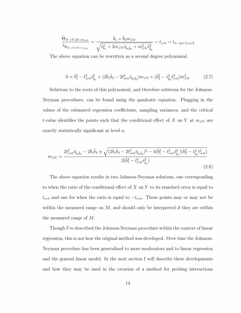
The above equation can be rewritten as a second degree polynomial.

0 = b21 − t2crits2

b1+ (2b1b3 − 2t2critsb1b3)mJN + (b2

3 − s2b3t2crit)m

2JN (2.7)

Solutions to the roots of this polynomial, and therefore solutions for the Johnson-

Neyman procedures, can be found using the quadratic equation. Plugging in the

values of the estimated regression coefficients, sampling variances, and the critical

t-value identifies the points such that the conditional effect of X on Y at mJN are

exactly statistically significant at level α.

mJN =2t2critsb1b3 − 2b1b3 ±

√(2b1b3 − 2t2critsb1b3)

2 − 4(b21 − t2crits2

b1)(b2

3 − s2b3t2crit)

2(b21 − t2crits2

b1)

(2.8)

The above equation results in two Johnson-Neyman solutions, one corresponding

to when the ratio of the conditional effect of X on Y to its standard error is equal to

tcrit and one for when the ratio is equal to −tcrit. These points may or may not be

within the measured range on M , and should only be interpreted if they are within

the measured range of M .

Though I’ve described the Johnson-Neyman procedure within the context of linear

regression, this is not how the original method was developed. Over time the Johnson-

Neyman procedure has been generalized to more moderators and to linear regression

and the general linear model. In the next section I will describe these developments

and how they may be used in the creation of a method for probing interactions

14

between a categorical variable with three or more levels and a continuous moderator,

providing an omnibus test of group differences at different values of a moderator.

A Brief History of the Johnson-Neyman Procedure

The Johnson-Neyman procedure was developed within the framework of analysis

of covariance (Johnson & Neyman, 1936; Johnson & Fay, 1950). The original ap-

proach was developed in a two-group two-moderator model. They began by defining

a linear model of the outcome variable of interest for two groups, group A and B:

E(YA) = a0 + a1Xi + a2Zi

E(YB) = b0 + b1Xi + b2Zi

Here YA and YB are the outcome variables for group A and B respectively. The

variables X and Z are moderators measured for each individual/case. The lower case

a’s and b’s are weights, estimated using a least squares criterion. The question was

then posed: For what values of X and Z are the expected values of YA and YB the

same and for which are they different? Johnson and Neyman derive the sums of

squares (SSFull) for a model where the expected values of YA and YB are different

at specified values of X and Z, x and z, and the sums of squares (SSreduced) for a

model where the expected values are fixed to be equal at x and z. Note that SSFull

does not depend on the choice of x and z, because there are no constraints on this

model. However, SSreduced is a function of x and z. This is equivalent to asking if

there is an effect of group (A vs. B) for individuals with the specific observed values

x and z. They define a sufficient statistic to test this question, the ratio between

the two calculated sums of squares (SSFull/SSreduced) whose cumulative distribution

15

function is the incomplete beta function, under the null hypothesis of no difference

in expected values at x and z. Johnson and Neyman define a critical value of the

incomplete beta function, as a function of some test level α, then derive the region

for which SSFull/SSreduced will be smaller than that critical value. This region is

defined as the region of significance and defines the region(s) of the range of the two

moderators X and Z for which the expected values of YA and YB differ. Of particular

importance in this method is the curve which limits the region of significance, which

is defined by the points at which SSFull/SSreduced exactly equals the critical value as

defined by α. This curve is frequently referred to as the boundary of significance.

Extensions of the Johnson-Neyman procedure within the ANCOVA framework

allowed for increased use of this method. The original work described only two mod-

erators, but Johnson and Hoyt (1947) generalized this approach to three moderators.

Abelson (1953) proposed that instead of always using the Johnson-Neyman proce-

dure, researchers should test if the regression slopes are the same for each group (a

test of moderation) and only proceed with the Johnson-Neyman procedure if this hy-

pothesis is rejected. Otherwise researchers can use ANCOVA. Additionally, Abelson

(1953) derived formulas for both the region of significance and the boundary of sig-

nificance for any number of moderators. Potthoff (1964) proposed the first approach

for dealing with more than two groups. He derived a simultaneous Johnson-Neyman

solution for all pairwise comparisons of groups.

There have been a few proposed methods for how to treat multiple groups when

using the Johnson-Neyman procedure. Huitema (1980) proposed using the proce-

dure for each pair of groups, thus defining regions of significance for each pair of

16

groups. Potthoff (1964) derived a simultaneous method for these pairwise compar-

isons. However both of these approaches can result in a large number of regions,

the interpretation of which can be difficult with an increasing number of groups. It

could be useful for researchers to know where along the range of a moderator the

groups differ from each other using an omnibus test of differences. Some research

based on the general linear model (Hunka, 1995; Hunka & Leighton, 1997), provided

equations for an omnibus region of significance with multiple groups in matrix form,

which will be used in my derivations later. However, the closed form solutions for the

region of significance were not provided, but rather, given a set of data the region of

significance was solved for using Mathematica, a fairly expensive program which is

not commonly used within psychology. Additionally, no more than three-groups were

considered, which may be the upper limit of this method for finding omnibus groups

differences.

An important extension of the Johnson-Neyman procedure moved away from just

categorical independent variables and into the framework of multiple regression, which

can include a categorical or continuous independent variable. Bauer and Curran

(2005) were the first to derive the Johnson-Neyman procedure for a continuous by

continuous variable interaction. They derived Equations 2.5 – 2.8, providing closed

form equations for solutions to the Johnson-Neyman boundary of significance and

thus the regions of significance. Bauer and Curran (2005) continue by deriving the

approximate Johnson-Neyman boundary of significance for linear multilevel models.

Preacher, Curran, and Bauer (2006) followed up with an online tool to calculate

Johnson-Neyman boundaries of significance for multiple linear regression, multilevel

17

models, and latent curve analysis. Hayes and Matthes (2009) generalized this ap-

proach to logistic regression, where the outcome is dichotomous. These publications

together allow for many applications to continuous independent variables in a variety

of different types of models.

These innovations and easy to use tools have allowed for the Johnson-Neyman

procedure to be applied in more varied contexts, increasing the versatility of this type

of analysis. Since its conception, researchers from a variety of academic fields have

published in applied journals encouraging their colleagues to consider the Johnson-

Neyman procedure as an alternative to ANCOVA or the simple-slopes method for

probing moderation effects, including education (Carroll & Wilson, 1970), nursing

(D’Alonzo, 2004), ecology (Engqvist, 2005), psychology (Hayes & Matthes, 2009),

and marketing (Spiller et al., 2013). Adoption of this method has been encouraged by

the development of a variety of computational tools to assist researchers in conducting

these analyses.

2.2.3 Tools for Probing

Probing an interaction by hand is often computationally intense and allows for

many opportunities for mistakes and rounding errors. A number of researchers have

created tools which take the computational burden, and potential for error, off of

the researcher. The first computational tool available for the Johnson-Neyman pro-

cedure was developed in the language TELCOMP (Carroll & Wilson, 1970). With

input summary statistics, the program could solve for the region of significance in a

two-group two-moderator problem, boasting a run time of a mere half hour. Code

for computing the Johnson-Neyman points for a dichotomous independent variable

18

in both SPSS and BDMP was provided in Karpman (1983) and expanded to SAS

in Karpman (1986). Pedhazur (1997) and O’Connor (1998) provided programs com-

patible for SPSS and SAS which computed simple-slopes analysis for two- and three-

way interactions. Preacher et al. (2006) provide an online tool which takes a vari-

ety of inputs generated from a traditional statistical package and can output both

simple-slopes and Johnson-Neyman solutions for multiple linear regression, hierarchi-

cal linear models, and latent curve analysis. The first within-package tool for SPSS

and SAS which could compute both simple-slopes and the Johnson-Neyman proce-

dure for continuous and dichotomous outcome variables was MODPROBE (Hayes &

Matthes, 2009). Most of the capabilities of MODPROBE have since been integrated

into PROCESS, a tool for SPSS and SAS which estimates moderation, mediation,

and conditional process models (Hayes, 2013).

Probing interactions is an important part of understanding how an the effect

of the independent variable on an outcome looks and behaves along the range of the

moderator. Methods for probing interactions (simple-slopes and the Johnson-Neyman

procedure) as well as accompanying tools for these methods have been available for

a number of years. Since there has not previously been a method for implementing

the Johnson-Neyman technique with categorical independent variables, I will provide

a tool to conduct the analysis, reducing the burden on the researcher.

19

Chapter 3: Moderation of the Effect of a Categorical

Variable

There are many instances where researchers are interested in moderation and

the predictor of interest X is categorical, such as race or religion or experimental

condition (when there are more than two conditions). For example, Barajas-Gonzales

and Brooks-Gunn (2014) investigated the relationship between participants’ ethnicity

(White, Black, or Latino) and fear of safety in their neighborhood. They proposed

that some ethnic groups may be more reactive to neighborhood disorder than other

groups, resulting in an interaction between ethnicity and neighborhood disorder in

predicting fear for safety. In a different study, Niederdeppe, Shapiro, Kim, Bartolo,

and Porticella (2014) had participants read one of three narratives about a woman’s

experience with weight loss, where each story varied how much personal responsibility

she took for her inability to lose weight (categorized as low, moderate, and high).

Participants then indicated their support for a variety of government policies which

might help individuals lose weight (e.g., increasing sidewalks in neighborhoods). They

found that story narrative had essentially no effect among those high in liberal beliefs,

but individuals low in liberal beliefs were more supportive of policies when the woman

in the story took low or moderate responsibility for her weight loss. Many other

examples of moderation of the effect of a categorical variable can be found throughout

20

psychology and other social sciences (e.g., Cleveland et al., 2013; O’Malley, Voight,

Renshaw, & Eklund, 2015).

In this chapter I describe how to make inference about moderation when X is

categorical, focusing particularly on the case where X has three or more categories.

Just as in the case of a continuous or dichotomous X, probing a moderation effect

is key to understanding how the effect of X on Y changes across the range of M . I

will describe the currently available methods for probing these types of interactions

in this chapter, leaving the development of the Johnson-Neyman procedure for the

following chapter.

3.1 Inference about Moderation

In the categorical case, X can be represented in linear regression using k − 1

variables, where k is the number of categories in X. There are a number of ways

to code X into these new variables, one of the most popular of which is dummy

coding (also known as indicator coding). Dummy coding is a method which recodes a

categorical variable into k−1 dichotomous variables which take the value of either 0 or

1 depending on which group the case is in. Each of the k−1 variables corresponds to

a specific group in X, with one group lacking a corresponding variable. If participant

i is in group j then the dummy variable corresponding to group j will equal 1 and

all other dummy variables will equal zero for case i. The one group which does not

have a corresponding dummy variable is often referred to as the reference group, and

individuals in this group have scores of zero on all dummy variables. An example of

dummy coding is provided below, where D1 corresponds to participants in Group 1,

21

D2 corresponds to participants in Group 2, D3 corresponds to participants in Group

3, and participants in Group 4 are the reference group.

X D1 D2 D3

1 1 0 02 0 1 03 0 0 14 0 0 0

I will continue throughout the manuscript under the assumption that dummy

codes are being used to describe the categorical variable of interest. However, any

other kind of coding can be used without loss of generality.

As in the case of two groups, researchers interested in testing questions of moder-

ation can set up two competing models, one model where the effect of X (now coded

in the D variables) is not contingent on some moderator M and another model where

the effect of X is contingent on M . Let us consider the example of three groups.

Because the effect of X is now captured by 2 variables (D1 and D2), the effect of each

of these variables should be allowed to be contingent on M as such:

Model 1: Yi = b∗0 + b∗1D1i + b∗2D2i + b∗3Mi + ε∗i

Model 2: Yi = b0 + ΘD1→Y |MD1i + ΘD2→Y |MD2i + b3Mi + εi

ΘD1→Y |M = b1 + b4Mi

ΘD2→Y |M = b2 + b5Mi

Here the effect of D1 and the effect of D2 are linear functions of M . By plugging

in the equations for ΘD1→Y |M and ΘD2→Y |M and expanding, the equation for Model

2 can be re-expressed as:

Yi = b0 + b1D1i + b2D2i + b3Mi + b4MiD1i + b5MiD2i + εi (3.1)

22

From Equation 3.1 it is clear that Model 1 is nested under Model 2, in that if both

b4 and b5 are zero, then Model 2 is equivalent to Model 1. Most regression software

does not provide results for simultaneous inference about multiple coefficients in the

model, but rather provides inferences about each coefficient on its own. However,

similar to the two group case, hierarchical regression analysis can be used to test if

adding the product termsD1M andD2M to Model 1 explains additional variance in Y

(i.e., if the joint hypothesis that both b4 and b5 are zero can be rejected). This type of

analysis can be completed using most statistical packages which can estimate linear

regression models. If the product terms explain a significant portion of additional

variance as assessed by applying Equation 2.1 and associated hypothesis tests, then

this is evidence that the relationship between X and Y is indeed contingent on M .

If there are more than three groups, additional dummy coded variables are needed,

and thus additional conditional relationships will be needed to fully quantify the

conditional relationship between X and Y . For example, Model 2 for a four group

case would be written as such:

Model 2: Yi = b0 + ΘD1→Y |MD1i + ΘD2→Y |MD2i + ΘD3→Y |MD3i + b4Mi + εi

ΘD1→Y |M = b1 + b5Mi

ΘD2→Y |M = b2 + b6Mi

ΘD3→Y |M = b3 + b7Mi

3.2 Probing Moderation Effects

Just like in the continuous or dichotomous case, a test of moderation is often

insufficient for answering all the questions a researcher may pose. For example, Nei-

derdeppe et al. (2014) may be interested in identifying the range of scores on their

23

political ideology scale (liberal – conservative) which correspond to significant differ-

ences among the story narratives. Methods for probing moderation of the relationship

between a categorical independent variable and a continuous outcome have been dis-

cussed in some books and publications (e.g., Cohen et al., 2003; Darlington & Hayes,

2017; Spiller et al., 2013), but not nearly as much as in the dichotomous or contin-

uous independent variable case. Specifically, what differentiates the categorical case

is that there is not always a single function which can describe the conditional effect

of X on Y , but rather k − 1 functions which must be taken together to describe the

conditional effect of X on Y .

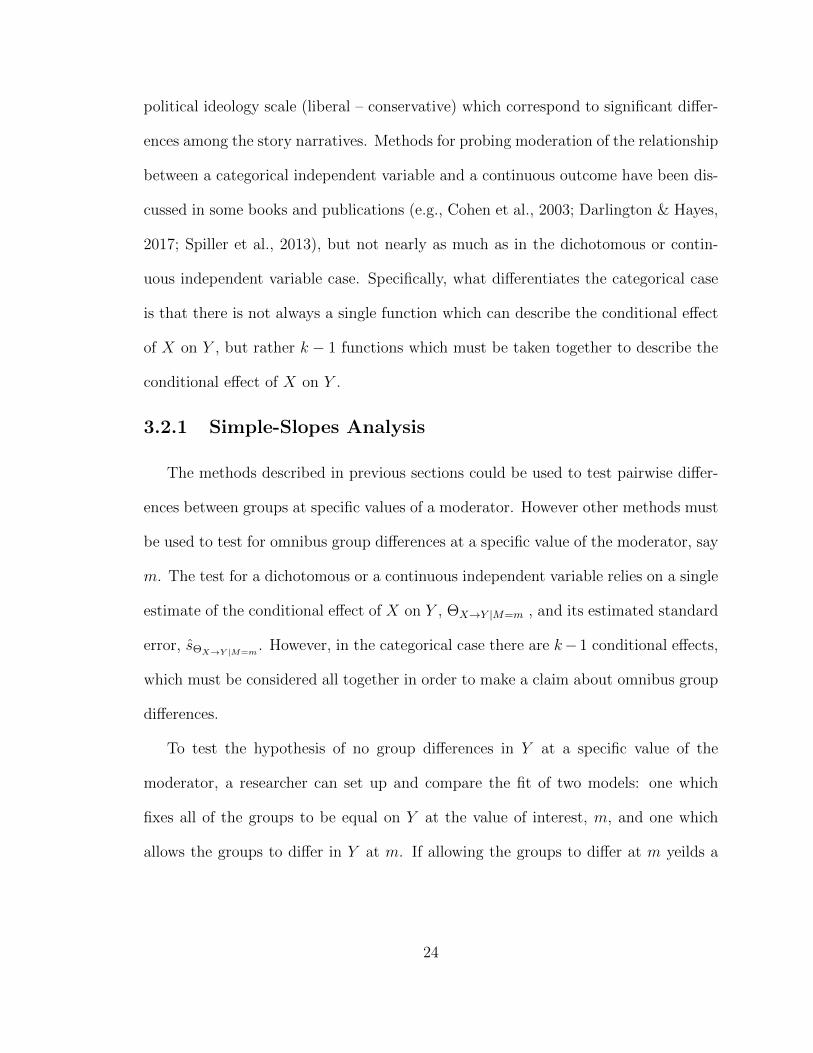
3.2.1 Simple-Slopes Analysis

The methods described in previous sections could be used to test pairwise differ-

ences between groups at specific values of a moderator. However other methods must

be used to test for omnibus group differences at a specific value of the moderator, say

m. The test for a dichotomous or a continuous independent variable relies on a single

estimate of the conditional effect of X on Y , ΘX→Y |M=m , and its estimated standard

error, sΘX→Y |M=m. However, in the categorical case there are k−1 conditional effects,

which must be considered all together in order to make a claim about omnibus group

differences.

To test the hypothesis of no group differences in Y at a specific value of the

moderator, a researcher can set up and compare the fit of two models: one which

fixes all of the groups to be equal on Y at the value of interest, m, and one which

allows the groups to differ in Y at m. If allowing the groups to differ at m yeilds a

24

better fitting model of Y , then this supports the claim that the groups vary on Y at

m, and thus there is an omnibus effect of X on Y at M = m.

To decide how to set up these models, let us examine the interpretations of the

regression coefficients in Equation 3.1. The interpretation of b1 is the predicted change

in Y with a one unit change in D1 when M is zero. When D1 is a dummy coded

variable, this indicates the estimated difference in Y between the group coded with

D1 and the reference group when M is zero. Similarly, when using dummy coding, b2

is the estimated difference in Y between the group coded with D2 and the reference

group when M is zero. Therefore, when both b1 and b2 are zero, there are no group

differences when M is zero.

A researcher could use hierarchical regression to test if b1 and b2 are both zero by

setting up one model which fixes b1 and b2 to be zero, and one that allows them to

vary.

Model 1: Yi = b∗0 + b∗1Mi + b∗2D1iMi + b∗3D2iMi + ε∗i

Model 2: b0 + b1D1i + b2D2i + b3Mi + b4D1iMi + b5D2iMi + εi

From the above equations it is clear that Model 1 is nested within Model 2,

where if b1 and b2 both equal zero in Model 2 then Model 2 is the same as Model 1.

Using hierarchical regression, estimate Model 1 then Model 2. If Model 2 explains

significantly more variance in Y than Model 1, this is evidence that b1 and b2 are not

both equal to zero, and thus there are group differences at the point where M is equal

to zero.

Based on this method it is easy to probe the effect of X and Y when M = 0.

Instead, we would like a general method for probing at any value of M , not just

25

M = 0. In order to probe the effect of X on Y at any point along M , say m, a

researcher should center the variable M at m, call this new variable M c = M − m

and use the same hierarchical regression method as above.

Model 1: Yi = b∗0 + b∗1Mci + b∗2D1iM

ci + b∗3D2iM

ci + ε∗i

Model 2: b0 + b1D1i + b2D2i + b3Mci + b4D1iM

ci + b5D2iM

ci + εi

It is now clear how to test for group differences in Y at any value of the moderator.

This method is equivalent to the simple-slopes method for two conditions, and would

result in the same conclusions as the method described above if used for a dichotomous

predictor X.

Though intuitive to some, it may be more clear to explain why re-centering works.

This can be described in the form of a model comparison, where one model fixes the

group differences in Y to be zero at m and the other allows the groups to vary at m.

The unconstrained model does not depend on the value of m chosen. However, by

beginning with the unconstrained model it is possible to derive the constrained model

in a general form, showing why the re-centering strategy proposed above works. The

unconstrained model for three groups can be described as such:

Yi = b0 + ΘD1→Y |MD1i + ΘD2→Y |MD2i + b3Mi + εi (3.2)

ΘD1→Y |M = b1 + b4Mi

ΘD2→Y |M = b2 + b5Mi

Because the question of interest is if the effect of X on Y is zero at m, constrain

both ΘD1→Y |M=m and ΘD2→Y |M=m to be zero.

26

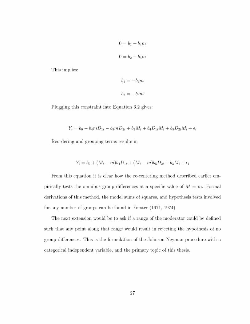
0 = b1 + b4m

0 = b2 + b5m

This implies:

b1 = −b4m

b2 = −b5m

Plugging this constraint into Equation 3.2 gives:

Yi = b0 − b4mD1i − b5mD2i + b3Mi + b4D1iMi + b5D2iMi + εi

Reordering and grouping terms results in

Yi = b0 + (Mi −m)b4D1i + (Mi −m)b5D2i + b3Mi + εi

From this equation it is clear how the re-centering method described earlier em-

pirically tests the omnibus group differences at a specific value of M = m. Formal

derivations of this method, the model sums of squares, and hypothesis tests involved

for any number of groups can be found in Forster (1971, 1974).

The next extension would be to ask if a range of the moderator could be defined

such that any point along that range would result in rejecting the hypothesis of no

group differences. This is the formulation of the Johnson-Neyman procedure with a

categorical independent variable, and the primary topic of this thesis.

27

Chapter 4: Derivations of the Johnson-Neyman Procedure

for Multiple Groups

Using an application of the approach to the Johnson-Neyman procedure in linear

regression from Bauer and Curran (2005) and the principles of hypothesis tests for

sets of regression coefficients, I will derive the boundary of significance for an omnibus

test of group difference along some moderator M . I begin with the derivation for three

groups and continue with a partial derivation for four groups. The solution for two

groups relies on solving for the roots of a two-degree polynomial, achieved easily by

applying the quadratic equation. The derivation of the Johnson-Neyman boundary

of significance for the three-group case relies on solving for the roots of a fourth-

degree polynomial, for which closed form solutions are available. In the four-group

derivation, the roots of an eighth-degree polynomial are required. The Abel-Ruffini

theorem states that there are no algebraic solutions for the roots of polynomials of

degree five or more (Abel, 1824; Ruffini, 1799). To deal with the issue of no closed

form algebraic solution for the boundary of significance I provide an iterative computer

program that solves for the Johnson-Neyman boundaries for any number of groups.

28

4.1 Three Groups

The region of significance is the range of the moderator such that any point within

that range results in rejecting the null hypothesis that there are no group differences

in Y at that point. These points can be described as those where allowing ΘD1→Y |M=m

and ΘD2→Y |M=m to be non-zero explains a significant amount of variance in Y . The

test of significance for the increase in variance explained is based on an F statistic

which can be calculated using Equation 2.1. This equation can be rewritten using

matrix algebra, and in this form I will use it to derive the boundaries of significance

in the three-group case.

F =(L′β)(L′ΣβL)−1(L′β)

q(4.1)

Recall from Chapter 2 that p is the number of predictors in the unconstrained

model, and q is the number of constraints made to the unconstrained model to results

in the constrained model. In the case of three groups q = 2. Here L′ is a q × (p+ 1)

matrix which describes the model constraints under the null hypothesis. β is a (p +

1)× 1 column vector containing the OLS estimates of the regression coefficients from

Model 2. Σβ is the estimated variance-covariance matrix of the regression coefficients

of size (p+ 1)× (p+ 1).

First consider the original data matrix, X. This matrix is not used in any of

the further equations, but it is important to note that formatting the data matrix in

this way results in the interpretations of the estimated regression coefficients below

matching the equations used above, particularly Equation 4.1.

29

X =

1 D11 D21 M1 D11M1 D21M1

1 D12 D22 M2 D12M2 D22M2...

......

......

...1 D1n D2n Mn D1nMn D2nMn

The corresponding regression coefficient estimates from Model 2 would be

β′ =[b0 b1 b2 b3 b4 b5

]Because the null hypothesis is that ΘD1→Y |M=m = b1 + b4m = 0 and ΘD2→Y |M=m =

b2 + b5m = 0 our contrast matrix L is defined as

L′ =

[0 1 0 0 m 00 0 1 0 0 m

]It may not be initially clear why L has been chosen in this manner, but once L′β

is examined, it is clear that the estimates of the functions of interest ΘD1→Y |M=m and

ΘD2→Y |M=m are defined by this contrast matrix.

L′β =

[b1 + b4m

b2 + b5m

]Additionally, because the individual variance and covariance components will be

integral to these derivations, Σβ will be defined as

Σβ =

v0 c01 c02 c03 c04 c05

c01 v1 c12 c13 c14 c15

c02 c12 v2 c23 c24 c25

c03 c13 c23 v3 c34 c35

c04 c14 c24 c34 v4 c45

c05 c15 c25 c35 c45 v5

Here the estimated sampling variance of each regression coefficient is defined by

the variable v with same subscript as the regression coefficient. For example, the

estimated sampling variance of b4 is v4. Similarly, the estimated sampling covariance

30

of two regression coefficients is noted by the variable c with the same subscripts as

regression coefficients. For consistency, the smallest subscript is always listed first.

For example, the estimated sampling covariance of b1 and b5 is noted as c15.

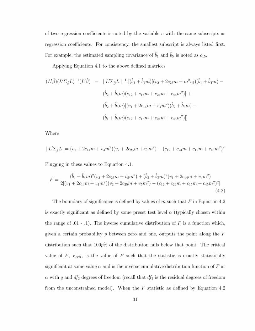
Applying Equation 4.1 to the above defined matrices

(L′β)(L′ΣβL)−1(L′β) = | L′ΣβL |−1 [(b1 + b4m)[(v2 + 2c25m+m2v5)(b1 + b4m)−

(b2 + b5m)(c12 + c15m+ c24m+ c45m2)] +

(b2 + b5m)[(v1 + 2c14m+ v4m2)(b2 + b5m)−

(b1 + b4m)(c12 + c15m+ c24m+ c45m2)]]

Where

| L′ΣβL |= (v1 + 2c14m+ v4m2)(v2 + 2c25m+ v5m

2)− (c12 + c24m+ c15m+ c45m2)2

Plugging in these values to Equation 4.1:

F =(b1 + b4m)2(v2 + 2c25m+ v5m

2) + (b2 + b5m)2(v1 + 2c14m+ v4m2)

2[(v1 + 2c14m+ v4m2)(v2 + 2c25m+ v5m2)− (c12 + c24m+ c15m+ c45m2)2]

(4.2)

The boundary of significance is defined by values of m such that F in Equation 4.2

is exactly significant as defined by some preset test level α (typically chosen within

the range of .01 - .1). The inverse cumulative distribution of F is a function which,

given a certain probability p between zero and one, outputs the point along the F

distribution such that 100p% of the distribution falls below that point. The critical

value of F , Fcrit, is the value of F such that the statistic is exactly statistically

significant at some value α and is the inverse cumulative distribution function of F at

α with q and df2 degrees of freedom (recall that df2 is the residual degrees of freedom

from the unconstrained model). When the F statistic as defined by Equation 4.2

31

is exactly equal to Fcrit, this statistic will be exactly significant, and thus values of

m such that F as defined in Equation 4.2 is equal to Fcrit define the boundary of

significance.

To find the boundary of significance, plug in Fcrit and q and solve for m. By

plugging in these values, setting the left hand side equal to zero, and reorganizing

terms it is clear that this equation is a fourth-degree polynomial in m.

0 = (b21v2 + b2

2v1 + 2Fcritv1v2c212) +

2[c23b21 + b1b4v2 + c14b

22 + b2b5v1 + 2Fcrit(c12c24 + c12c15 − v1c25 − v2c14)]m+

[v5b21 + 4c25b1b4 + b2

4v2 + v4b22 + 4c14b2b5 + b2

5v1 +

2Fcrit(2c45c12 + c224 + 2c24c15 + c2

15 − v1v5 − 4c14c25 − v22)]m2 +

2[v5b1b4 + c25b24 + v4b2b5 + c14b

25 + 2Fcrit(c24c45 + c15c45 − v5c14 − c25v2)]m3 +

[v5b24 + v4b

25 − 2Fcritv2v5c

245]m4 (4.3)

The solutions for the roots of this equation are long algebraic equations. There

are four solutions, some of which may be imaginary depending on specific values of

the regression coefficients, variances, and covariances. Below is one of the solutions.

In order to simplify notation, let each coefficient from Equation 4.3 be equal to some

variable.

d = b21v2 + b2

2v1 + Fcrit2v1v2

e = 2[c23b21 + b1b4v2 + c14b

22 + b2b5v1 + 2Fcrit(c12c24 + c12c15 − v1c25 − v2c14)]

f = v5b21 + 4c25b1b4 + b2

4v2 + v4b22 + 4c14b2b5 + b2

5v1 +

2Fcrit(2c45c12 + c224 + 2c24c14 + c2

15 − v1v5 − 4c14c25 − v22)

g = 2[v5b1b4 + c25b24 + v4b2b5 + c14b

25 + 2Fcrit(c24c25 + c15c45 − v5c14 − c25v2)]

32

h = v5b24 + v4b

25 − 2Fcritv2v5

Using these new variables the solution for one root of Equation 4.3 can be ex-

pressed algebraically. This is the first Johnson-Neyman solution, mJN1 . For the sake

of brevity, and because these equations would typically be implemented in a computer

program, there is no need to express the other roots. They are all of a similar form,

based completely off the variables d, e, f , g, and h.

MJN1 = − g

4h+

1

2(g2

4h2− 2f

3h+

1

6h(−288dfh+ 108dg2 + 108e2h− 36efg + 8f 3 +

12(−768d3h3 + 576d2egh2 + 384d2f 2h2 − 432d2fg2h+

81d2g4 − 432de2fh2 + 18de2g2h+ 240def 2gh− 54defg3 − 48df 4h+

12df 3g2 + 81e4h2 − 54e3fgh+ 12e3g3 + 12e2f 3h− 3e2f 2g2)1/2)1/3 +

2

3(12dh− 3eg + f 2)/(h(−288dfh+ 108dg2 + 108e2h− 36efg + 8f 3 +

12(−768d3h3 + 576d2egh2 + 384d2f 2h2 − 432d2fg2h+ 81d2g4 −

432de2fh2 + 18de2g2h+ 240def 2gh− 54defg3 − 48df 4h+ 12df 3g2 +

81e4h2 − 54e3fgh+ 12e3g3 + 12e2f 3h− 3e2f 2g2)1/2)1/3))1/2 +

1

2(g2

2h2− 4f

3h− 1

6h(−288dfh+ 108dg2 + 108e2h− 36efg + 8f 3 +

12(−768d3h3 + 576d2egh2 + 384d2f 2h2 − 432d2fg2h+ 81d2g4 −

432de2fh2 + 18de2g2h+ 240def 2gh− 54defg3 − 48df 4h+ 12df 3g2 +

81e4h2 − 54e3fgh+ 12e3g3 + 12e2f 3h− 3e2f 2g2)1/2)1/3 −

2

3(12dh− 3eg + f 2)/(h(−288dfh+ 108dg2 + 108e2h− 36efg + 8f 3 +

12(−768d3h3 + 576d2egh2 + 384d2f 2h2 − 432d2fg2h+ 81d2g4 −

432de2fh2 + 18de2g2h+ 240def 2gh− 54defg3 − 48df 4h+ 12df 3g2 +

33

81e4h2 − 54e3fgh+ 12e3g3 + 12e2f 3h− 3e2f 2g2)1/2)1/3) +

(fg

h2− 2e

h− g3

4h3)/(

g2

4h2− 2f

3h+

1

6h(−288dfh+ 108dg2 + 108e2h−

36efg + 8f 3 + 12(−768d3h3 + 576d2egh2 + 384d2f 2h2 − 432d2fg2h+

81d2g4 − 432de2fh2 + 18de2g2h+ 240def 2gh− 54defg3 − 48df 4h+

12df 3g2 + 81e4h2 − 54e3fgh+ 12e3g3 + 12e2f 3h− 3e2f 2g2)1/2)1/3 +

2

3(12dh− 3eg + f 2)/(h(−288dfh+ 108dg2 + 108e2h− 36efg + 8f 3 +

12(−768d3h3 + 576d2egh2 + 384d2f 2h2 − 432d2fg2h+ 81d2g4 −

432de2fh2 + 18de2g2h+ 240def 2gh− 54defg3 − 48df 4h+ 12df 3g2 +

81e4h2 − 54e3fgh+ 12e3g3 + 12e2f 3h− 3e2f 2g2)1/2)1/3))1/2)1/2

Using the solutions for the roots of quartic equations, the solutions for the Johnson-

Neyman boundary of significance for a test of omnibus group differences in the case

of three groups are well defined.

Though these equations are notably complicated, they are not too unwieldy to be

programmed into a computer program, such as an SPSS or SAS macro or R-package,

to solve for the Johnson-Neyman boundaries of significance for linear regression prob-

lems with a continuous moderator and a three-group categorical variable. A computer

program that implements this solution would be greatly useful to researchers inter-

ested in omnibus group differences which are moderated by a continuous variable.

These solutions will be able to inform them of the range of the moderator variable

which defines significant group differences and non-significant group differences.

Though this is the first time an algebraic solution has been derived for the three-

groups case, it would be ideal to provide a general solution for any number of groups.

34

In order to investigate this as a possibility, I perform a similar derivation using the

same equations and an expanded contrast matrix for the four-group case.

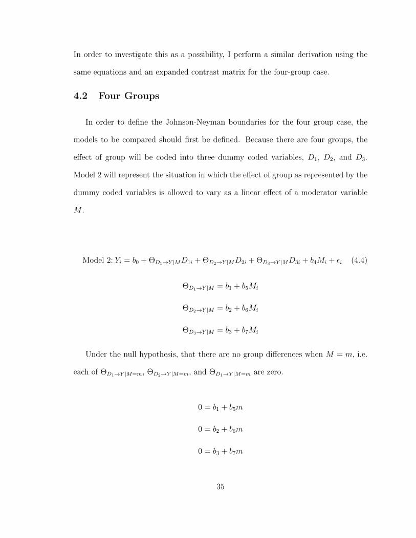
4.2 Four Groups

In order to define the Johnson-Neyman boundaries for the four group case, the

models to be compared should first be defined. Because there are four groups, the

effect of group will be coded into three dummy coded variables, D1, D2, and D3.

Model 2 will represent the situation in which the effect of group as represented by the

dummy coded variables is allowed to vary as a linear effect of a moderator variable

M .

Model 2: Yi = b0 + ΘD1→Y |MD1i + ΘD2→Y |MD2i + ΘD3→Y |MD3i + b4Mi + εi (4.4)

ΘD1→Y |M = b1 + b5Mi

ΘD2→Y |M = b2 + b6Mi

ΘD3→Y |M = b3 + b7Mi

Under the null hypothesis, that there are no group differences when M = m, i.e.

each of ΘD1→Y |M=m, ΘD2→Y |M=m, and ΘD1→Y |M=m are zero.

0 = b1 + b5m

0 = b2 + b6m

0 = b3 + b7m

35

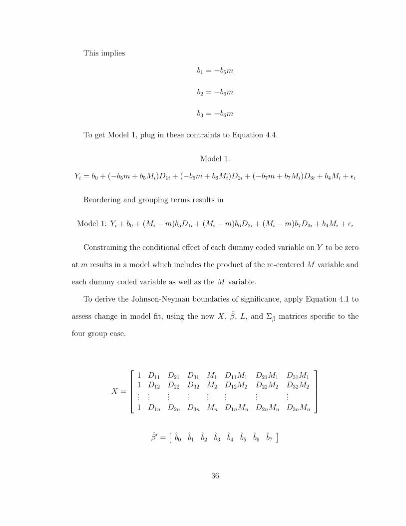
This implies

b1 = −b5m

b2 = −b6m

b3 = −b6m

To get Model 1, plug in these contraints to Equation 4.4.

Model 1:

Yi = b0 + (−b5m+ b5Mi)D1i + (−b6m+ b6Mi)D2i + (−b7m+ b7Mi)D3i + b4Mi + εi

Reordering and grouping terms results in

Model 1: Yi + b0 + (Mi −m)b5D1i + (Mi −m)b6D2i + (Mi −m)b7D3i + b4Mi + εi

Constraining the conditional effect of each dummy coded variable on Y to be zero

at m results in a model which includes the product of the re-centered M variable and

each dummy coded variable as well as the M variable.

To derive the Johnson-Neyman boundaries of significance, apply Equation 4.1 to

assess change in model fit, using the new X, β, L, and Σβ matrices specific to the

four group case.

X =

1 D11 D21 D31 M1 D11M1 D21M1 D31M1

1 D12 D22 D32 M2 D12M2 D22M2 D32M2...

......

......

......

...1 D1n D2n D3n Mn D1nMn D2nMn D3nMn

β′ =[b0 b1 b2 b3 b4 b5 b6 b7

]

36

L′ =

0 1 0 0 0 m 0 00 0 1 0 0 0 m 00 0 0 1 0 0 0 m

Σβ =

v0 c01 c02 c03 c04 c05 c06 c07

c01 v1 c12 c13 c14 c15 c16 c17

c02 c12 v2 c23 c24 c25 c26 c27

c03 c13 c23 v3 c34 c35 c36 c37

c04 c14 c24 c34 v4 c45 c46 c47

c05 c15 c25 c35 c45 v5 c56 c57

c06 c16 c26 c36 c46 c56 v6 c67

c07 c17 c27 c37 c47 c57 c67 v7

Based on these equations, the product of L′ and β define the model constraints of

interest.

L′β =

b1 + b5m

b2 + b6m

b3 + b7m

Applying Equation 4.1 to the above defined matrices

(L′β)′(L′ΣβL)−1(L′β) =

| L′ΣβL |−1 [(b1 + b5m)2[(v2 + 2c26m+ v6m

2)(v3 + 2c37m+ v7m2)− (c23 +

c36m+ c27m+ c67m2)2]− (b1 + b5m)(b2 + b6m)[(c12 + c25m+ c16m+ c56m

2)(v3 +

2c37m+ v7m2) + (c13 + c35m+ c17m+ c57m

2)(c23 + c27m+ c36m+ c67m2)] +

(b1 + b5m)(b3 + b7m)[(c12 + c25m+ c16m+ c56m2)(c23 + c36m+ c27m+ c67m

2)−

(c13 + c25m+ c17m+ c57m2)(v2 + 2c26m+ v6m

2)]− (b1 + b5m)(b2 + b6m)[(c12 +

c25m+ c16m+ c56m2)(v3 + 2c37m+ v7m

2) + (c13 + c35m+ c17m+ c57m2)(c23 +

c27m+ c36m+ c67m2)] + (b2 + b6m)2[(v1 + 2c15m+ v5m

2)(v3 + 2c37m+ v7m2)−

(c13 + c35m+ c17m+ c57m2)2] + (b2 + b6m)(b3 + b7m)[(c13 + c35m+ c17m+

37

c57m2)(c12 + c16m+ c25m+ c56m

2)− (v1 + 2c15m+ v5m2)(c23 + c36m+ c27m+

c67m2)] + (b1 + b5m)(b3 + b7m)[(c12 + c25m+ c16m+ c56m

2)(c23 + c36m+ c27m+

c67m2)− (c13 + c35m+ c17m+ c57m

2)(v2 + 2c26m+ v6m2)] + (b2 + b6m)(b3 +

b7m)[(c13 + c35m+ c17m+ c57m2)(c12 + c16m+ c25m+ c56m

2)− (v1 + 2c15m+

v5m2)(c23 + c36m+ c27m+ c67m

2)] + (b3 + b7m)2[(v1 + 2c15m+ v5m2)(v2 +

2c26m+ v6m2)− (c12 + c25m+ c16m+ c36m

2)2]]

Where

| L′ΣβL | = (v1 + 2mc15 + v5m2)(v2 + 2c26m+ v6m

2)(v3 + 2c37m+ v7m2)− (v1 +

2c15m+ v5m2)(c23 + c36m+ c27m+ c67m

2)(c23 + c27m+ c36m+

c67m2)− (c12 + c25m+ c16m+ c56m

2)2(v3 + 2c37m+ v7m2) + 2(c12 +

c25m+ c16m+ c56m2)(c23 + c36m+ c27m+ c67m

2)(c13 + c17m+

c35m+ c57m2)− (c13 + c17m+ c35m+ c57m

2)(v2 + 2c26m+ v6m2)

Again, F is defined as a polynomial function of m as in the three condition case.

A polynomial for which the roots would determine the Johnson-Neyman boundary

of significance can be defined by setting F to its critical value given the degrees of

freedom in this problem, and setting one side of the equation to zero. In doing this

(though excluded for the sake of space) this polynomial is an eighth degree polynomial

in m. By the Abel-Ruffini theorem (1824) there is no closed form algebraic solution

for the roots of this equation, thus precluding the derivation of the solutions for the

Johnson-Neyman boundary of significance. Hunka (1995) and Hunka and Leighton

(1997) proposed the use of Mathematica to apply these matrix calculations given

a specific data set. Their examples, however, only examined up to three-groups,

38

and Mathematica cannot calculate the roots of all equations of degree five or higher

(“Roots”, n.d.). This means that the methods proposed by Hunka and colleagues are

limited to three-groups or fewer.

Without a method for finding the Johnson-Neyman boundary of significance in

the four-condition case, it may seem that a solution for finding these boundaries in

a general number of groups is far out of reach. However, it is possible to probe

interactions between continuous variables and categorical variables of any number of

categories using the simple-slopes method. A computer program could repeatedly

probe the effect of some categorical variable, honing in on the point at which group

differences in Y are exactly significant, thus defining the Johnson-Neyman region of

significance without a closed-form solution. For my thesis I developed such a tool,

available in two popular statistical packages to increase the potential user base of the

tool.

39

Chapter 5: OGRS: An Iterative Tool for Finding

Johnson-Neyman Regions of Significance for Omnibus Group

Differences

OGRS (Omnibus Groups Regions of Significance) is an easy to use tool which

can probe interactions between a categorical independent variable and a continuous

moderator. It is available for two popular statistical packages, SPSS and SAS. After

executing the OGRS macro, users will be able to specify a single OGRS command

line that specifies all the information needed to do the analyses, while requiring no

mathematics on the part of the user. The tool will produce typical regression output,

the Johnson-Neyman boundaries of significance, and a table which describes how the

effect of the independent variable changes across the observed range of the moderator.

See Appendix A and B for SPSS code and documentation, and Appendix C and D

for SAS code and documentation.

5.1 Program Inputs

Each language has a different syntax structure for the OGRS command line, but

the required inputs are the same across both the SPSS and SAS versions. The only

exception is that SAS requires a data file name, whereas SPSS assumes that the active

dataset is the one being analyzed. The only required inputs are the variables involved

40

in the analysis. Optional inputs include confidence level, convergence criteria, and

number of initial iterations in the Johnson-Neyman algorithm.

5.1.1 Required Inputs

OGRS requires only one variable as the independent variable in the subcommand

X. Researchers should save their independent variable as one variable with each group

having a unique code (e.g., 1 = Protestant, 2 = Catholic, 3 = Jewish, etc). OGRS

recodes this variable into k − 1 dummy codes internally for use in regression. Only

one variable each will be accepted as input for the moderator and for the outcome

variable. Additional covariates can also be included by specifying them in the vars

command, but not assigning them to any specific role (X, Y, or M). There is no limit

to the number of covariates allowed in the model.

Below are examples of the base command line for each language.

SPSS OGRS vars = var1 var2 var3 var4 var5 /X = var1 /M = var2

/Y = var3.

SAS %OGRS (data = datafile, vars = var1 var2 var3 var4 var5,

X = var1, M = var2, Y = var3);

The list of variables in the vars subcommand, specifies all the variables that

are used in the regression. Including this command allows researchers to specify

additional covariates that do not play the role of independent variable, moderator, or

outcome.

5.1.2 Optional Inputs

A few options have been built into OGRS to increase its flexibility and allow

users to troubleshoot issues with the Johnson-Neyman algorithm. Researchers can

specify the level of confidence, the convergence criteria used by the Johnson-Neyman

41

algorithm, the number of initial iterations in the Johnson-Neyman algorithm, and the

number of decimal places printed in the output. Each of these options has a default

value that can be overridden by specifying the name of the subcommand then an

equals sign and the new value which is desired (e.g., CONF = 92).

Confidence Level

Confidence level is used in two parts of the OGRS routine. In the regression

output, confidence intervals are provided alongside each of the estimated regression

coefficients. The confidence level specified in the OGRS command line is used to

determine the level of confidence at which these intervals are calculated. The default

is 95. The users can specify any confidence level greater than 50 and less than 100 in

the CONF subcommand. The second part of the OGRS routine which uses confidence

level is the Johnson-Neyman algorithm. The Johnson-Neyman algorithm searches

for the point along the continuous range of the moderator at which the effect of

the independent variable on the outcome variable is exactly statistically significant.

This significance level is determined by the confidence level specified in the CONF

subcommand. For example, when the confidence level is set at 90, then the p-value

corresponding to the effect of the independent variable on the outcome variable at

the Johnson-Neyman boundary of significance will be .10. Similarly if the confidence

level is specified to be 99, the p-value will be .01.

Convergence Criteria

The convergence criteria is used to calibrate how close the Johnson-Neyman algo-

rithm gets to the exact answer. The default is as precise as the language is capable:

.00000001 (up to eight decimal places in both SPSS and SAS). However, if a researcher

42

is not particularly concerned with the exactness of the solution, then they can specify

a more relaxed convergence criteria.

The convergence criteria means different things in each of the languages. In SAS,

OGRS looks to converge to a critical F statistic, but in SPSS, OGRS converges

to an α level (reasons for this are discussed in the next section). The statistic to

which the routine aims to converge, whether it be an F statistic or an α value,

will be called the criterion statistic, and the desired value of that statistic will be

called the criterion value. In each of the languages, the default is to find a point

that has a corresponding criterion statistic which is within eight decimal places of

the criterion value. By specifying a different value in the CONVCRIT subcommand,

a solution that is that distance (or a smaller distance) from the criterion value will

be deemed acceptable. For example if a user specified CONVCRIT = .0001 then a

solution within four decimal points of the criterion value would be acceptable. This

can be useful for reducing runtime, as will be discussed later, or if the measurement

scale of the variable is not particularly precise, so that the solution does not need to

be particularly precise.

Initial Iterations

As discussed in Section 5.5, the Johnson-Neyman algorithm begins by dividing

the range of the moderator into sections. The number of sections the space is divded

into is determined by the iter subcommand. The default for the number of sections

is 50 + k ∗ 10, where k is the number of groups in the independent variable. As

will be discussed later, there is a trade off between speed of the program and finding

all Johnson-Neyman solutions. Researchers who are particularly concerned about

making sure they find all the solutions, but do not care about how long it takes the

43

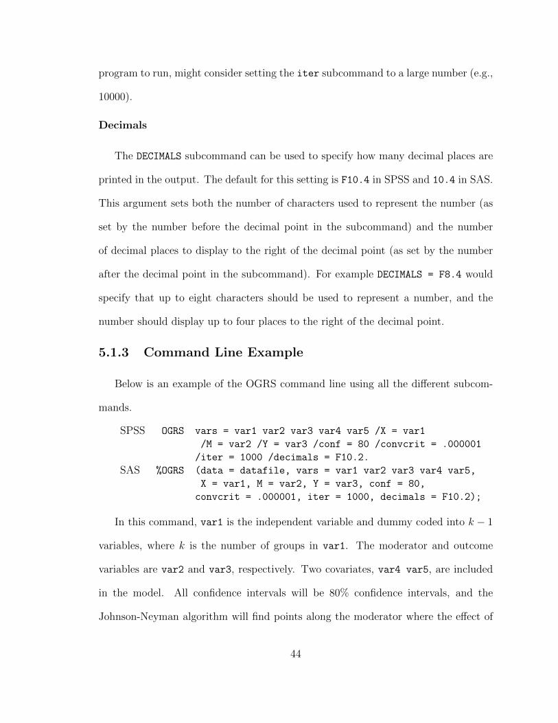
program to run, might consider setting the iter subcommand to a large number (e.g.,

10000).

Decimals

The DECIMALS subcommand can be used to specify how many decimal places are

printed in the output. The default for this setting is F10.4 in SPSS and 10.4 in SAS.

This argument sets both the number of characters used to represent the number (as

set by the number before the decimal point in the subcommand) and the number

of decimal places to display to the right of the decimal point (as set by the number

after the decimal point in the subcommand). For example DECIMALS = F8.4 would

specify that up to eight characters should be used to represent a number, and the

number should display up to four places to the right of the decimal point.

5.1.3 Command Line Example

Below is an example of the OGRS command line using all the different subcom-

mands.

SPSS OGRS vars = var1 var2 var3 var4 var5 /X = var1

/M = var2 /Y = var3 /conf = 80 /convcrit = .000001

/iter = 1000 /decimals = F10.2.

SAS %OGRS (data = datafile, vars = var1 var2 var3 var4 var5,

X = var1, M = var2, Y = var3, conf = 80,

convcrit = .000001, iter = 1000, decimals = F10.2);

In this command, var1 is the independent variable and dummy coded into k − 1

variables, where k is the number of groups in var1. The moderator and outcome

variables are var2 and var3, respectively. Two covariates, var4 var5, are included

in the model. All confidence intervals will be 80% confidence intervals, and the

Johnson-Neyman algorithm will find points along the moderator where the effect of

44

the independent variable on the outcome is exactly statistically significant at α = .20.

Acceptable solutions for the algorithm will be within .000001 of the criterion value,

whether it is an F -statistic in SAS or a p-value in SPSS. Initially, the algorithm will

divide the range of the moderator into 1000 sections, which will be used to find the

solutions, as described below. All output will be reported up to two decimal places.

5.2 Internal Processes

The OGRS routine uses the information provided in the command line to calculate

all the information needed to create the output. For example, OGRS can detect the

number of groups in the variable input in the X subcommand. This will imply the

number of groups, which will be important throughout. Additionally the range of the

moderator will be defined by the variable input in the M subcommand. The iterative

approach to the Johnson-Neyman procedure will only search within the observed

range of the moderator, as this is the only well-defined space where the researcher

has measurements.

5.2.1 Regression Results

After recoding the variable specified in the X subcommand, the program will

estimate the regression model using all the variables in the vars subcommand with

the exception of the variable in the Y subcommand, to predict the variable specified in

the Y subcommand, including all product terms between the M variable and the codes

representing X. All regression coefficients, standard errors, and inferential statistics

including t and p-values and confidence intervals are computed and appear in the

output. Additionally, a section of output at the bottom of the regression results is

dedicated to the test of interaction, comparing the contingent (including all product

45

terms between the dummy codes for X and M) and non-contingent models (not

including any of the product terms).

5.2.2 Finding Johnson-Neyman Solutions

Since it is not possible to directly solve for M such that the associated F statistic

reflecting group differences is exactly significant, an alternative is to search for values

of M such that this is true. An iterative method to examine a variety of values of

M can be used to complete this task. The method for finding the Johnson-Neyman

boundaries of significance is based on the bi-section method, a popular method in

computer science for finding roots of polynomials.

The Bi-Section Method

The bi-section method is a method for iteratively searching for the point along a

closed range where some continuous function equals a prespecified value. In this case

we are looking at the function which determines either the p-value associated with

the test of the effect of X on Y at different M values (SPSS), or the associated F

statistic (SAS). Either way, these functions are both continuous.

The intermediate value theorem states that if the values of this function at the

boundaries of the range of the domain of the function span the criterion value, then

there is some point where the function is exactly the criterion value within that range.

In our case, if we can find two values of the moderator where the criterion statistic

is below the criterion value, and another value of the moderator where the criterion

statistic is above the criterion value, then somewhere in between those points, the F

statistic is exactly the criterion value. This is the principle upon which the bi-section

method is based.

46

The bi-section method assumes that you start with a continuous function where

the range of the domain is such that the value of the function at the minimum of the

domain is less than (or greater than) the criterion value, and the value of the function

at the maximum of the domain is greater than (or less than) the criterion value value.

Under this assumption, the bi-section method continuously divides the space in half,

evaluating the function at the divided point, then chooses a half which still spans the

criterion value until a point which is close enough the criterion value is found.

In the Johnson-Neyman algorithm, we cannot ensure that we have two points

which span the criterion value (as there may be no such points), so we divide the

space up in small sections, increasing the likelihood that we find two points which

span the criterion value, if such points exist. The algorithm then repeatedly applies

the bisection method to find the Johnson-Neyman boundaries of significance.

Implementation in OGRS Routine

Using the results from the regression analysis, all of the matrices used in Equa-

tion 4.1 are completely known with the exception of L, which contains an unknown

m. To search the space along the moderator’s range, a jump parameter is specified

that divides the range of the moderator. The jump parameter is the width of jump

required to span the space of the moderator in a set number of jumps equal to the

iter subcommand, where the default is 50 + 10 ∗ k, where k is the number of groups

in the independent variable.

The program will identify the range of the moderator and divide this range into

sections, solving for the statistical significance of the group differences in Y at each

endpoint of the sections. The program will then identify specific sections that transi-

tion between significance and non-significance (i.e. sections where one endpoint has

47

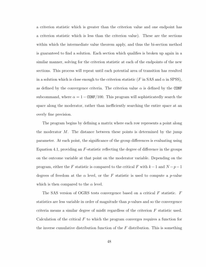
a criterion statistic which is greater than the criterion value and one endpoint has

a criterion statistic which is less than the criterion value). These are the sections

within which the intermediate value theorem apply, and thus the bi-section method

is guaranteed to find a solution. Each section which qualifies is broken up again in a

similar manner, solving for the criterion statistic at each of the endpoints of the new

sections. This process will repeat until each potential area of transition has resulted

in a solution which is close enough to the criterion statistic (F in SAS and α in SPSS),

as defined by the convergence criteria. The criterion value α is defined by the CONF

subcommand, where α = 1− CONF/100. This program will sophisticatedly search the

space along the moderator, rather than inefficiently searching the entire space at an

overly fine precision.

The program begins by defining a matrix where each row represents a point along

the moderator M . The distance between these points is determined by the jump

parameter. At each point, the significance of the group differences is evaluating using

Equation 4.1, providing an F -statistic reflecting the degree of difference in the groups

on the outcome variable at that point on the moderator variable. Depending on the

program, either the F statistic is compared to the critical F with k−1 and N −p−1

degrees of freedom at the α level, or the F statistic is used to compute a p-value

which is then compared to the α level.

The SAS version of OGRS tests convergence based on a critical F statistic. F

statistics are less variable in order of magnitude than p-values and so the convergence

criteria means a similar degree of misfit regardless of the criterion F statistic used.

Calculation of the critical F to which the program converges requires a function for

the inverse cumulative distribution function of the F distribution. This is something

48

that SAS has built into PROC IML, which is the language used to program OGRS.

However, the SPSS matrix language does not have a similar function. I investigated

a few approximations to this function (Abamowitz & Stegun, 1964; Bratley, Fox, &

Schrage, 1983); however, the approximations were off by enough that it seemed more

reasonable to use the α value instead of the approximate critical-F .

Areas of transition are identified by tagging (in an additional column of the matrix)

points where the criterion statistc was less than the specified criterion value in the

row above and is now greater than the specified criterion value, or rows where the

row above was greater than the criterion value and is now less than the criterion

value (i.e. the statistic has transitioned from significant to non-significant or non-

significant to significant). The program then checks if either of the two rows involved

in the transition converge based on the convergence criteria, and if either does, it

does not investigate this area further. When neither of these points is close enough

to converge, the program will examine this space on the moderator in more detail.

When a transition area is identified, the program identifies the boundaries of M

in this area and divides this range using the same number of jumps as before. Within

this space all previous calculations are repeated (Using Equation 4.1 to calculate an

F -statistic, and p-value) for each point. This new matrix of results is then inserted

into the original results matrix, and the program continues to look for other areas of

transition.

Areas are repeatedly searched with greater and greater precision until a solution

which is close enough to the criterion value based on the convergence criteria is found.

After this solution is found, the program will move on to a new transition area, if

one exists. Depending on the number of groups, the number of potential transition

49

areas will be limited (with only two potential transitions in 2 group, and 4 potential

transitions in 3 groups, etc). The program will continue until each area of transition

has a subsequent solution. There is currently no maximum number of times the

program can divide up a specific space within OGRS.

5.3 Program Outputs

Figure 6.1 provides an example of the output from OGRS for SPSS. The program

output includes regression results, Johnson-Neyman results, and a table which shows

how the effect of the independent variable on the outcome changes across the mod-

erator. The output begins with a section specifying the variables in the analyses,

including X, M , Y , and any covariates. There is also a table which shows how X was

dummy coded into k−1 variables. Next there is a section with the regression results.

This includes all the regression coefficient estimates, standard errors, t-statistics, p-

values, and confidence intervals. At the end of the regression results section is the

results of comparing the model with no interactions to the model with interactions,

and the associated test of significance which is a test of moderation.

The Johnson-Neyman results are presented with a table. The points of transition

are printed above the table. After the transition points, a table of other points

is provided to give the users a sense of the trends in the change in R2 and the

associated F statistic across the range of M . Approximately 20 lines are printed

in the table. This table could be used to graph the change in R2 or the associated

F -statistic across the range of the moderator in order to describe how the effect of

the independent variable on the outcome variable changes across this range.

50

5.4 Programming Decisions

Many programming decisions were made through testing and limitations of lan-

guages used. I will first outline the major decisions, then overview some of the testing

processes and performance outcomes which drove these decisions.

One of the major concerns was how the program would identify when there are

no Johnson-Neyman solutions. OGRS probes the initial points as determined by the

iter subcommand, and if these points do not identify any transition points, then

the program is complete and prints a message which states there are no Johnson-

Neyman solutions. During testing, most solutions were identified even with a very

small number of initial iterations. In most tested cases, all solutions were identified

using only three iterations. However, some specific cases emerged where two solu-

tions were very close together, and thus were not identified with a small number of

iterations. The largest number of iterations that did not find all solutions in all test

cases was 30. Additionally, the number of possible solutions increases as the number

of groups increases. This led to the decision to set the default number of iterations to

50 + 10k. This would allow for well over 30, which was the minimally sufficient case

in testing. Additionally, as will be seen in the run-time performance results, having

too many iterations caused the program to run quite slowly. It is very difficult to

choose a default for the number of iterations such that there are enough to identify

all transition points but not so many as to cause the program to run slowly. This

led me to add in the option for researchers to change the number of iterations. That

way if the program is running particularly slowly, they can decrease the number of

iterations, or if they are concerned that the algorithm missed some solutions, they

can increase the number of iterations.

51

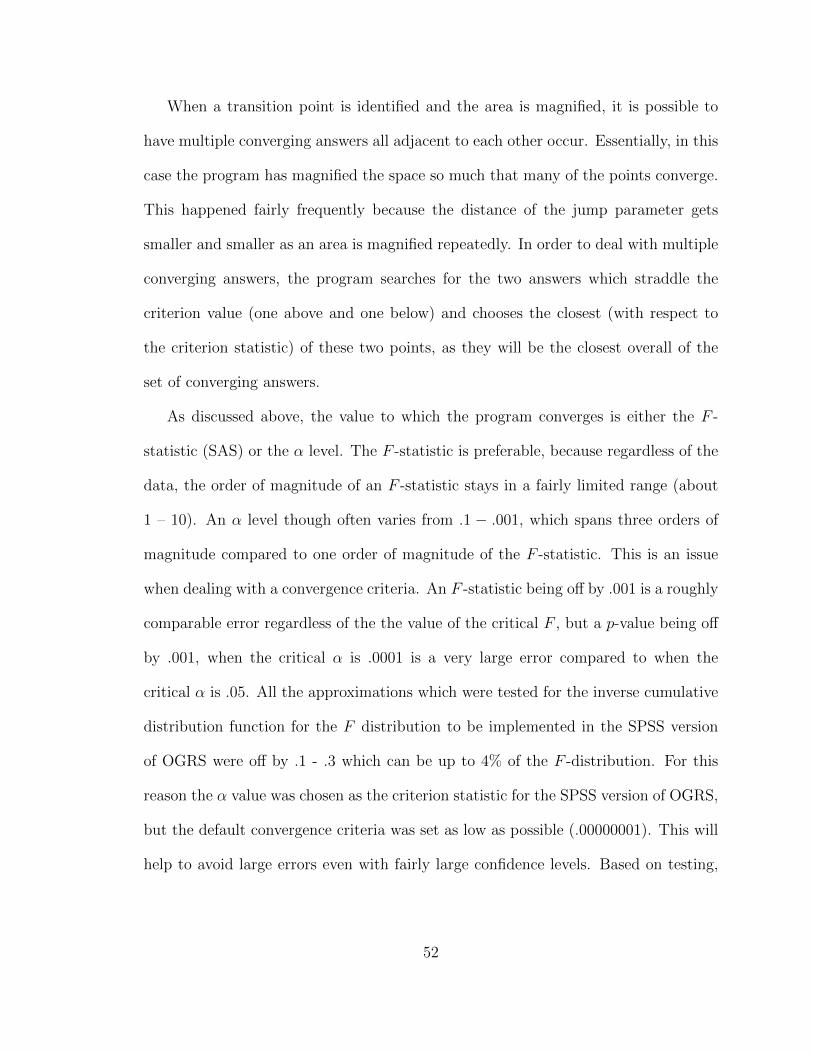
When a transition point is identified and the area is magnified, it is possible to

have multiple converging answers all adjacent to each other occur. Essentially, in this

case the program has magnified the space so much that many of the points converge.

This happened fairly frequently because the distance of the jump parameter gets

smaller and smaller as an area is magnified repeatedly. In order to deal with multiple

converging answers, the program searches for the two answers which straddle the

criterion value (one above and one below) and chooses the closest (with respect to

the criterion statistic) of these two points, as they will be the closest overall of the

set of converging answers.

As discussed above, the value to which the program converges is either the F -

statistic (SAS) or the α level. The F -statistic is preferable, because regardless of the

data, the order of magnitude of an F -statistic stays in a fairly limited range (about

1 – 10). An α level though often varies from .1 − .001, which spans three orders of

magnitude compared to one order of magnitude of the F -statistic. This is an issue

when dealing with a convergence criteria. An F -statistic being off by .001 is a roughly

comparable error regardless of the the value of the critical F , but a p-value being off

by .001, when the critical α is .0001 is a very large error compared to when the

critical α is .05. All the approximations which were tested for the inverse cumulative

distribution function for the F distribution to be implemented in the SPSS version

of OGRS were off by .1 - .3 which can be up to 4% of the F -distribution. For this

reason the α value was chosen as the criterion statistic for the SPSS version of OGRS,

but the default convergence criteria was set as low as possible (.00000001). This will

help to avoid large errors even with fairly large confidence levels. Based on testing,

52

convergence criteria influenced run time, but not drastically, so it seemed reasonable

to set this value to be very low.

Next, I will discuss some of the program tests which were completed in order

to understand the limitations of OGRS as well as make some of the programming

decisions above.

5.5 Program Performance

There were three major aspects of the program that I wanted to test. The first

two are accuracy related: 1) When does the program miss certain answers or get

answers that are incorrect, and 2) How accurate are the answers that the program

gets. The third aspect of the program is understanding how long it takes to run in

a variety of circumstances and understanding what influences how long the program

runs.

5.5.1 Accuracy

Perhaps the most important characteristic of an approximation is that is it ac-

curate enough to be useful. Though I cannot decide for potential users whether

or not this method is accurate enough to be useful, I can provide some information

about how accurate this method is, and potential users can decide whether this seems

accurate enough.

Accuracy comes in two forms with this algorithm. The algorithm must identify

the correct transition points (and not points that are not transition points) and it

must estimate those transition points well. Different parts of the algorithm come into

play for these two different types of accuracy so I will treat them separately.

53

Finding Solutions

Finding the correct solutions is determined by whether or not the initial number

of iterations is large enough to ensure there are points spanning each transition point.

Having these spanning points is what ensures the bi-section method will work, but

there is no way to know for sure if all transition points have been identified. If two

solutions are contained within one region of the initial division of the range of the

moderator, then those solutions will not be found. Because of this it is important to

have a sufficient number of initial iterations.

To test how many iterations seems sufficient, I used datasets with 3, 5, and 7

groups, sample sizes of 20, 100, and 1000, and covergence criteria of 10−8 and 10−4,

and iterations of 3, 4, 5, 10, 20, 30, 40, 50, 100, 1000, and 10000. These datasets

were also used to test runtimes. In Tables 5.2 to 5.4 there are rows with asterisks

which indicate the iteration numbers which failed to find the correct Johnson-Neyman

boundaries of significance. As can be seen from Tables 5.2 to 5.4 the largest value

which failed to find the correct Johnson-Neyman boundary in any of the conditions

was 30. Though, this may be an artifact of the data generation procedure, and there

is no true lower bound on how close two Johnson-Neyman boundaries could be. So

there is no way to know completely that all solutions have been found, regardless of

the number of initial iterations selected.

Because 30 was the upper bound of the number of iterations which did not find all

Johnson-Neyman boundaries of significance when testing, I selected 50 as the default

minimum number of iterations with additional iterations added based on the number

of groups. More groups have more possible solutions, and therefore two solutions

may be more likely to be close to each other. When using OGRS, I also recommend

54

making a visualization of the effect of the relationship between X and Y across M ,

such that you might be able to notice if a two transition points have been skipped,

as this would likely show up on a graph as a quick change in the group differences.

There were no situations where a solution was found that was not a Johnson-

Neyman transition point. Because of the way the algorithm is written there is no

reason to suspect this might occur. The major issue of inaccuracy that could occur

is for two transition points to be skipped.

Accuracy of Solutions

Though this algorithm has been developed to provide solutions to the Johnson-

Neyman boundaries of significance for cases where there is no previously available

solution, it is important to test this algorithm in situations where the solutions are

known. Testing against known solutions allows us to understand better how accurate

the solutions are in known cases, and how accurate the solutions are even in the

unknown cases. Based on our previous discussion we know that closed form solutions

are available in the two and three condition case.

Table 5.1 provides the closed form solution for two randomly generated datasets.

The first dataset had two groups, and was generated to have two Johnson-Neyman

solutions. The second dataset had three groups, and was generated to have two

Johnson-Neyman solutions. The “true” solutions were calculated using Maple, an

analytical software with highly accurate algorithms for computing the roots of poly-

nomials. OGRS was used in SPSS and SAS with convergence criteria ranging from

10−2 to 10−8. In the cells of Table 5.1 are two values, the first value is the solution

from OGRS printed to eight decimal places, the second value is the proportion of the

range of the moderator by which the OGRS solution differs from the Maple solution.

55

For example, if the moderator ranged from -1 to 1, then the range would be 2. If

the Maple solution was 1.4 and the OGRS solution was 1.35. Then the difference

between the Maple solution and the OGRS solution would be 1.4− 1.35 = .05 which

is .05/2 = .025 or 2.5% of the range of the moderator. I used this statistic to describe

the error in the OGRS algorithm, as it is reasonable to suspect the amount of error

in the algorithm will be directly proportional to the scale of the moderator.

Based on Table 5.1 it seems that the algorithm is fairly accurate with the maximum

error being less than .5% of the range of the moderator. It does seem that the SAS

algorithm is slightly more accurate than the SPSS algorithm, particularly at higher

values of the convergence criteria. This is likely related to the different criterion

statistics used, where SAS uses an F -statistic and SPSS uses an α value. Additionally,

as expected the algorithm is more accurate when a lower convergence criteria is used.

It seems that the algorithm performs admirably, even with very high convergence

criteria. For researchers who believe that this level of accuracy is sufficient, they could

use OGRS to solve for Johnson-Neyman boundaries of significance using this tool.

Though we cannot test for the situations of four groups or more, it seems rea-

sonable to assume that the algorithm would remain accurate when there are more

groups. The major issue of additional groups is missing potential transition points,

and increased run time.

5.5.2 Run Time

Run times were recorded for both the SPSS and SAS version of OGRS using

27 different datasets. The datasets were randomly generated in GAUSS to be of

varying group number, sample size, and number of Johnson-Neyman solutions. Three

56

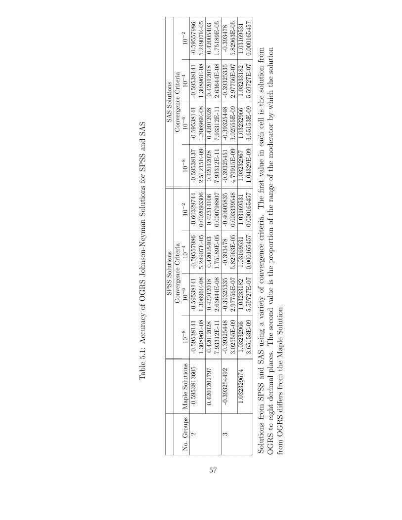
Tab

le5.

1:A

ccura

cyof

OG

RS

Joh

nso

n-N

eym

anSol

uti

ons

for

SP

SS

and

SA

S

SPSSSolutions

SASSolutions

Convergence

Criteria

Convergence

Criteria

No.

Groups

Map

leSolution

s10

−8

10−6

10−4

10−2

10−8

10−6

10−4

10−

2

2-0.5953813605

-0.59538141

-0.59538141

-0.59557986

-0.60329744

-0.59538137

-0.59538141

-0.59538141

-0.59557986

1.30896E

-08

1.30896E-08

5.24907E-05

0.002093306

2.51215E-09

1.30896E-08

1.30896E-08

5.24907E-05

0.4201202797

0.42012028

0.42012018

0.42005403

0.42314106

0.42012028

0.42012028

0.42012018

0.42005403

7.93312E

-11

2.63644E-08

1.75189E-05

0.000798807

7.93312E-11

7.93312E-11

2.63644E-08

1.75189E-05

3-0.393254492

-0.39325448

-0.39325335

-0.393478

-0.40605835

-0.39325451

-0.39325448

-0.39325335

-0.393478

3.02555E

-09

2.97756E-07

5.82963E-05

0.003339548

4.79915E-09

3.02555E-09

2.97756E-07

5.82963E-05

1.032329674

1.03232966

1.03233182

1.03169531

1.03169531

1.03232967

1.03232966

1.03233182

1.03169531

3.65153E

-09

5.59727E-07

0.000165457

0.000165457

1.04329E-09

3.65153E-09

5.59727E-07

0.000165457

Sol

uti

ons

from

SP

SS

and

SA

Susi

ng

ava

riet

yof

conve

rgen

cecr

iter

ia.

The

firs

tva

lue

inea

chce

llis

the

solu

tion

from

OG

RS

toei

ght

dec

imal

pla

ces.

The

seco

nd

valu

eis

the

pro

por

tion

ofth

era

nge

ofth

em

oder

ator

by

whic

hth

eso

luti

onfr

omO

GR

Sdiff

ers

from

the

Map

leSol

uti

on.

57

different group numbers were used: 3, 5, and 7. Three sample sizes were used: 20,

100, and 1000. Finally there were three different numbers of solutions generated: 0,

1, and 2. Each dataset was analyzed 22 times in each language using each of two

convergence criteria (10−8 and 10−4) and each of 11 different initial iterations: 3, 4,

5, 10, 20, 30, 40, 50, 100, 1000, 10000.

Run times were recorded by hand on a cellphone stopwatch while running SPSS

as there is not built in functional for timing in SPSS. The SAS program times each

executed statement, so the times were recorded after each run. Both programs were

run on a Dell Optiplex 745 computer running Windows 7 Enterprise with an Intel(R)

Core(TM) 2 CPU processor. During the tests no other programs or applications were

running.

Tables 5.2 to 5.4 contain all times for all conditions for both SPSS and SAS.

Because times of less than 1 second by hand were fairly unreliable in SPSS, the time

reported states “< 1”. Minimum run time was .22 seconds (3 Groups, Sample Size

100, convergence criteria 10−4, SAS, 3 initial iterations). Maximum run time was

1104 seconds or 18.39 minutes (5 Groups, Sample Size 1000, Convergence criteria

10−8, SAS, 10000 initial iterations).

The major finding from this experiment was that smaller numbers of initial iter-

ations took less time to run. However, smaller numbers of initial iterations are more

likely to miss potential solutions. Balancing these two findings was important when

setting the defaults for number of initial iterations. In general, a smaller number

of initial iterations resulted in fewer probed points required to find a point which

converged, leading to the quicker speed of these runs.

58

Datasets with more groups and larger samples took longer to analyze. This is

likely because the data matrix needed to be inverted is larger in both of these cases.

Inverting large matrices is time consuming even for computers. Especially when the

number of initial iterations was quite large, some of the larger datasets took multiple

minutes to run. Interestingly, though SAS was typically faster than SPSS, in some of

these large data and large initial iteration conditions, SPSS ran faster than SAS.

The number of solutions influenced run time slightly. When there are no solutions,

the program only checks the initial iterations then exits. In this situation the program

runs quite quickly, especially when there are few initial iterations. When there is one

solution, fewer magnifications must occur compared to when there are two solutions,

so typically more solutions resulted in higher run times.

Convergence criteria seemed to impact runtime slightly. With a higher conver-

gence criteria, fewer magnifications are required, and the program can run more

quickly. Though the program run more quickly with a higher convergence criteria,

lowering the convergence criteria impacts the accuracy of the solutions, and so the

default was set to the most accurate, as run times were still fairly reasonable under

this condition. If a researcher is particularly concerned about runtime and is willing

to sacrifice some accuracy, they can change the convergence criteria from the default.

Some of these run times are fairly unreasonable and might lead a user to assume

that their computer has crashed or the program is not working. As such, I chose the

initial value of iterations to reflect fairly reasonable run times. Even in the worst case

scenario tested (N = 1000, 7 Groups, and 2 Solutions) the default initial iterations

would be 120, which we would expect to run in about 6 - 12 seconds depending on

the language and convergence criteria. Additionally, by allowing the user to specify

59

the number of iterations, they can tailor the run time in cases where they have very

large datasets or feel the program is likely to run slowly.

Overall, the runtimes informed the default convergence criteria and number of

iterations. Keeping in mind a balance between accuracy and run time, I believe that

aiming for the program to run in a few seconds in most small data situations and in

under a minute in large data cases seemed reasonable. Researchers concerned that the

program will run too long can change the defaults to their situation. The measured

run times for this study were all on the same machine and are by no means universal.

Some machines will run slower or faster. Users of OGRS can tailor their command

line inputs to balance accuracy and speed on their own machine.

Next we will examine an application of OGRS to a real dataset. Through this

example, users can see how what the OGRS output will look like and also how to

interpret the output with respect to their research questions.

60

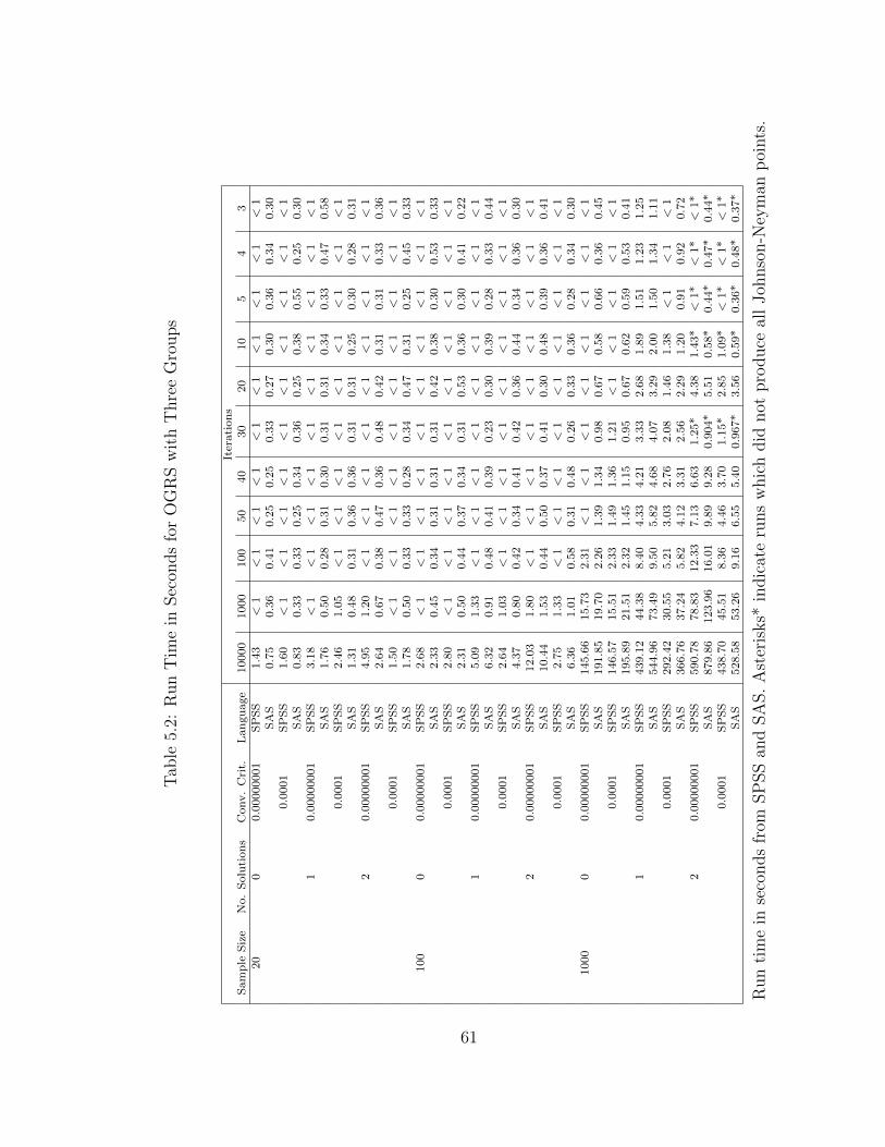
Tab

le5.

2:R

un

Tim

ein

Sec

onds

for

OG

RS

wit

hT

hre

eG

roups

Iter

ati

on

sS

am

ple

Siz

eN

o.

Solu

tion

sC

onv.

Cri

t.L

an

gu

age

10000

1000

100

50

40

30

20

10

54

320

00.0

0000001

SP

SS

1.4

3<

1<

1<

1<

1<

1<

1<

1<

1<

1<

1S

AS

0.7

50.3

60.4

10.2

50.2

50.3

30.2

70.3

00.3

60.3

40.3

00.0

001

SP

SS

1.6

0<

1<

1<

1<

1<

1<

1<

1<

1<

1<

1S

AS

0.8

30.3

30.3

30.2

50.3

40.3

60.2

50.3

80.5

50.2

50.3

01

0.0

0000001

SP

SS

3.1

8<

1<

1<

1<

1<

1<

1<

1<

1<

1<

1S

AS

1.7

60.5

00.2

80.3

10.3

00.3

10.3

10.3

40.3

30.4

70.5

80.0

001

SP

SS

2.4

61.0

5<

1<

1<

1<

1<

1<

1<

1<

1<

1S

AS

1.3

10.4

80.3

10.3

60.3

60.3

10.3

10.2

50.3

00.2

80.3

12

0.0

0000001

SP

SS

4.9

51.2

0<

1<

1<

1<

1<

1<

1<

1<

1<

1S

AS

2.6

40.6

70.3

80.4

70.3

60.4

80.4

20.3

10.3

10.3

30.3

60.0

001

SP

SS

1.5

0<

1<

1<

1<

1<

1<

1<

1<

1<

1<

1S

AS

1.7

80.5

00.3

30.3

30.2

80.3

40.4

70.3

10.2

50.4

50.3

3100

00.0

0000001

SP

SS

2.6

8<

1<

1<

1<

1<

1<

1<

1<

1<

1<

1S

AS

2.3

30.4

50.3

40.3

10.3

10.3

10.4

20.3

80.3

00.5

30.3

30.0

001

SP

SS

2.8

0<

1<

1<

1<

1<

1<

1<

1<

1<

1<

1S

AS

2.3

10.5

00.4

40.3

70.3

40.3

10.5

30.3

60.3

00.4

10.2

21

0.0

0000001

SP

SS

5.0

91.3

3<

1<

1<

1<

1<

1<

1<

1<

1<

1S

AS

6.3

20.9

10.4

80.4

10.3

90.2

30.3

00.3

90.2

80.3

30.4

40.0

001

SP

SS

2.6

41.0

3<

1<

1<

1<

1<

1<

1<

1<

1<

1S

AS

4.3

70.8

00.4

20.3

40.4

10.4

20.3

60.4

40.3

40.3

60.3

02

0.0

0000001

SP

SS

12.0

31.8

0<

1<

1<

1<

1<

1<

1<

1<

1<

1S

AS

10.4

41.5

30.4

40.5

00.3

70.4

10.3

00.4

80.3

90.3

60.4

10.0

001

SP

SS

2.7

51.3

3<

1<

1<

1<

1<

1<

1<

1<

1<

1S

AS

6.3

61.0

10.5

80.3

10.4

80.2

60.3

30.3

60.2

80.3

40.3

01000

00.0

0000001

SP

SS

145.6

615.7

32.3

1<

1<

1<

1<

1<

1<

1<

1<

1S

AS

191.8

519.7

02.2

61.3

91.3

40.9

80.6

70.5

80.6

60.3

60.4

50.0

001

SP

SS

146.5

715.5

12.3

31.4

91.3

61.2

1<

1<

1<

1<

1<

1S

AS

195.8

921.5

12.3

21.4

51.1

50.9

50.6

70.6

20.5

90.5

30.4

11

0.0

0000001

SP

SS

439.1

244.3

88.4

04.3

34.2

13.3

32.6

81.8

91.5

11.2

31.2

5S

AS

544.9

673.4

99.5

05.8

24.6

84.0

73.2

92.0

01.5

01.3

41.1

10.0

001

SP

SS

292.4

230.5

55.2

13.0

32.7

62.0

81.4

61.3

8<

1<

1<

1S

AS

366.7

637.2

45.8

24.1

23.3

12.5

62.2

91.2

00.9

10.9

20.7

22

0.0

0000001

SP

SS

590.7

878.8

312.3

37.1

36.6

31.2

5*

4.3

81.4

3*

<1*

<1*

<1*

SA

S879.8

6123.9

616.0

19.8

99.2

80.9

04*

5.5

10.5

8*

0.4

4*

0.4

7*

0.4

4*

0.0

001

SP

SS

438.7

045.5

18.3

64.4

63.7

01.1

5*

2.8

51.0

9*

<1*

<1*

<1*

SA

S528.5

853.2

69.1

66.5

55.4

00.9

67*

3.5

60.5

9*

0.3

6*

0.4

8*

0.3

7*

Run

tim

ein

seco

nds

from

SP

SS

and

SA

S.

Ast

eris

ks*

indic

ate

runs

whic

hdid

not

pro

duce

all

Joh

nso

n-N

eym

anp

oints

.

61

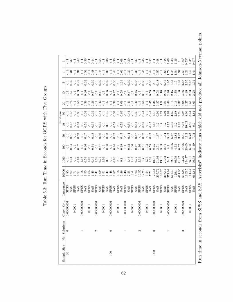
Tab

le5.

3:R

un

Tim

ein

Sec

onds

for

OG

RS

wit

hF

ive

Gro

ups

Iter

ati

on

sS

am

ple

Siz

eN

o.

Solu

tion

sC

onv.

Cri

t.L

an

gu

age

10000

1000

100

50

40

30

20

10

54

320

00.0

0000001

SP

SS

1.8

5<

1<

1<

1<

1<

1<

1<

1<

1<

1<

1S

AS

0.9

70.4

10.3

40.6

10.4

80.4

80.7

50.5

0.3

90.3

10.3

70.0

001

SP

SS

1.7

1<

1<

1<

1<

1<

1<

1<

1<

1<

1<

1S

AS

0.9

10.6

40.3

70.5

30.3

40.3

60.5

30.3

90.4

20.3

10.4

21

0.0

0000001

SP

SS

3.1

81.1

8<

1<

1<

1<

1<

1<

1<

1<

1<

1S

AS

1.9

50.5

90.3

60.4

70.5

60.3

10.3

90.3

60.3

30.5

90.3

60.0

001

SP

SS

1.8

51.0

3<

1<

1<

1<

1<

1<

1<

1<

1<

1S

AS

1.4

50.4

70.3

40.4

80.3

70.3

60.3

60.3

70.3

90.4

80.4

42

0.0

0000001

SP

SS

5.4

11.3

8<

1<

1<

1<

1<

1<

1<

1<

1<

1S

AS

3.0

90.7

20.3

70.3

60.3

90.4

10.4

20.4

10.3

90.4

50.5

50.0

001

SP

SS

1.9

11.0

4<

1<

1<

1<

1<

1<

1<

1<

1<

1S

AS

1.4

70.5

0.3

80.5

30.3

0.4

20.5

0.3

60.3

90.3

90.3

6100

00.0

0000001

SP

SS

3.4

8<

1<

1<

1<

1<

1<

1<

1<

1<

1<

1S

AS

2.8

70.6

60.4

40.4

20.5

10.3

70.3

90.4

70.3

60.4

40.3

60.0

001

SP

SS

3.1

8<

1<

1<

1<

1<

1<

1<

1<

1<

1<

1S

AS

2.8

60.8

0.3

90.4

50.5

90.6

21.0

80.5

81.3

10.6

62.0

81

0.0

0000001

SP

SS

6.4

31.8

1.1

<1

<1

<1

<1

<1

<1

<1

<1

SA

S7.5

51.4

30.4

20.4

40.5

90.4

10.4

10.4

70.3

90.3

90.3

90.0

001

SP

SS

3.4

1.4

31.0

6<

1<

1<

1<

1<

1<

1<

1<

1S

AS

5.2

30.7

70.4

70.4

70.4

40.3

90.4

20.4

50.3

80.3

90.3

72

0.0

0000001

SP

SS

10.5

52.3

41.1

6<

1<

1<

1<

1<

1<

1<

1<

1S

AS

12.2

81.7

0.5

10.6

20.3

90.4

10.5

60.3

10.3

60.4

50.4

50.0

001

SP

SS

3.5

41.7

61.0

3<

1<

1<

1<

1<

1<

1<

1<

1S

AS

7.7

11.3

30.5

50.4

20.4

50.4

40.4

50.5

90.3

60.4

40.5

21000

00.0

0000001

SP

SS

176.5

418.6

12.7

51.8

1.6

81.4

51.3

61.0

3<

1<

1<

1S

AS

207.7

221.3

62.5

11.3

71.2

0.9

40.8

70.5

80.4

80.5

50.4

80.0

001

SP

SS

185.2

519.3

13.3

31.9

11.7

1.7

11.3

1.1

6<

1<

1<

1S

AS

208.5

721.6

22.5

41.4

41.2

1.0

10.8

10.5

50.4

50.6

40.4

81

0.0

0000001

SP

SS

374.9

454.7

8.2

5.4

35.1

53.6

13.4

62.4

61.9

51.7

81.6

6S

AS

622.4

662.5

110.6

66.4

75.3

74.6

23.1

52.1

51.6

11.4

81.3

30.0

001

SP

SS

179.4

36.5

94.7

33.8

33.2

2.6

82.1

61.7

51.5

1.5

41.3

6S

AS

414.3

541.9

26.5

23.4

23.6

52.7

82.3

71.3

61.0

10.9

71

20.0

0000001

SP

SS

533.0

993.2

614.9

68.6

17.9

37.0

85.0

83.6

62.6

82.5

31.3

5*

SA

S1103.5

154.7

720.0

511.2

10.0

38.0

36.2

74.2

92.6

52.2

90.5

3*

0.0

001

SP

SS

114.4

756.0

16.8

86.7

34.8

63.4

43.5

12.5

32.1

32.4

1.3

*S

AS

661.8

466.5

811.3

97.9

36.4

4.8

13.6

52.2

51.5

11.4

40.6

7*

Run

tim

ein

seco

nds

from

SP

SS

and

SA

S.

Ast

eris

ks*

indic

ate

runs

whic

hdid

not

pro

duce

all

Joh

nso

n-N

eym

anp

oints

.

62

Tab

le5.

4:R

un

Tim

ein

Sec

onds

for

OG

RS

wit

hSev

enG

roups

Iter

ati

on

sS

am

ple

Siz

eN

o.

Solu

tion

sC

onv.

Cri

t.L

an

gu

age

10000

1000

100

50

40

30

20

10

54

320

00.0

0000001

SP

SS

2.7

41.3

31.3

1.2

1.1

81.2

51.1

31.0

61.3

51.2

1.2

SA

S0.9

20.5

30.3

90.4

20.4

80.3

60.3

0.5

20.3

40.4

40.5

90.0

001

SP

SS

2.4

41.4

31.3

31.2

61.1

41.2

1.1

81

11

1S

AS

0.9

40.5

90.3

40.3

10.5

20.3

70.3

90.4

20.3

40.3

10.4

71

0.0

0000001

SP

SS

4.0

41.5

61.3

1.3

61.2

51.3

61.2

11.2

51.2

31.3

1.3

6S

AS

2.2

10.6

90.5

50.3

60.4

80.3

90.4

50.5

60.4

10.3

60.6

70.0

001

SP

SS

2.5

11.5

11.3

81.2

51.2

61.3

11.2

81.2

61.2

11.2

31.2

6S

AS

1.5

50.6

70.3

40.3

40.5

0.3

40.3

30.5

50.3

70.3

30.4

72

0.0

0000001

SP

SS

6.9

1.8

31.6

1.2

11.2

81.2

61.1

61.2

1.2

11.3

11.3

1*

SA

S3.5

0.7

30.3

60.3

40.3

20.4

90.3

50.3

40.3

10.3

50.2

9*

0.0

001

SP

SS

2.5

11.5

61.3

1.3

11.3

31.3

61.1

51.3

91.3

91.3

51.3

6*

SA

S2.1

70.5

70.3

90.4

0.4

0.4

0.3

90.3

90.4

0.4

10.4

9*

100

00.0

0000001

SP

SS

4.5

31.7

1.6

41.2

41.3

81.3

61.4

31.4

51.3

81.4

31.4

3S

AS

3.0

50.6

40.3

90.3

60.5

0.3

50.4

80.3

40.3

40.4

40.3

60.0

001

SP

SS

4.6

11.7

81.4

11.4

31.3

61.4

11.3

31.3

91.3

81.3

81.5

3S

AS

3.1

0.6

60.4

40.6

0.4

30.3

40.3

50.3

70.3

20.3

50.3

31

0.0

0000001

SP

SS

8.2

32.5

61.7

61.6

51.4

51.7

1.5

1.3

81.4

61.5

61.5

8S

AS

8.5

91.4

50.5

0.4

70.4

60.4

40.4

20.3

90.3

90.4

70.3

80.0

001

SP

SS

4.7

3.2

51.6

31.6

61.3

11.3

1.3

51.5

61.2

51.5

51.2

8S

AS

5.7

90.8

80.3

90.3

60.3

90.3

60.3

50.3

10.3

30.6

30.3

42

0.0

0000001

SP

SS

12.5

63.3

11.8

41.6

61.7

81.7

1.5

31.6

1.5

91.5

91.5

8*

SA

S13.9

92.1

10.5

80.5

30.4

20.4

30.5

20.4

0.3

60.3

90.3

4*

0.0

001

SP

SS

4.8

2.5

61.9

61.6

1.8

1.6

81.4

1.7

61.6

11.6

11.5

8*

SA

S8.5

41.2

80.5

20.5

10.4

30.4

10.4

20.4

0.3

20.4

70.3

6*

1000

00.0

0000001

SP

SS

243.8

326.7

34.2

3.0

82.8

62.6

61.5

61.4

61.4

51.8

61.6

8S

AS

224.6

822.9

92.7

11.5

31.3

41.1

10.8

90.7

50.5

40.7

40.5

10.0

001

SP

SS

242.5

226.4

84.3

53.1

63.0

62.5

52.4

2.1

51.9

32

1.5

6S

AS

225.0

622.8

52.6

21.5

1.3

61.0

51

0.6

10.4

90.6

10.4

61

0.0

0000001

SP

SS

479.1

251.2

19.3

5.7

97.3

66.0

64.0

63.3

3.1

63.0

82.7

6S

AS

673.8

167.7

411.5

77.0

25.6

74.9

83.5

42.2

31.6

31.5

1.3

60.0

001

SP

SS

242.2

26.9

16.9

14.5

55.0

34.3

3.5

32.7

62.7

82.4

62.4

8S

AS

449.3

245.4

17.1

4.8

23.0

63.1

62.1

91.4

91.0

90.9

60.9

22

0.0

0000001

SP

SS

700.9

6116.5

618.0

112.2

9.6

32.6

6*

2.6

4*

2.3

3*

1.6

3*

2.3

*1.7

1*

SA

S895.3

3112.2

418.1

10.3

99.1

61.0

5*

0.8

3*

0.6

7*

0.5

*0.4

5*

0.5

*0.0

001

SP

SS

229.7

648.3

18.9

5.5

54.9

32.7

8*

2.4

8*

1.7

5*

2.2

4*

2.1

8*

2.2

*S

AS

448.3

267.6

19.5

65.9

65.0

41.1

6*

0.8

9*

0.7

8*

0.5

5*

0.5

6*

0.7

3*

Run

tim

ein

seco

nds

from

SP

SS

and

SA

S.

Ast

eris

ks*

indic

ate

runs

whic

hdid

not

pro

duce

all

Joh

nso

n-N

eym

anp

oints

.

63

Chapter 6: Party Differences in Support of Government

Action to Mitigate Climate Change

Climate change has been an increasing topic of discussion throughout science and

government. Particularly within psychology, it is important to understand who be-

lieves in climate change and who denies it. Through this example, we can investigate

how political party identification and age are related to support of government action

to mitigate climate change. In this study 815 U.S. citizens completed a survey online

related to their opinions about global warming in the U.S. These participants were

recruited such that they were approximately representative of the U.S. population.

The outcome I will examine in this dataset is a composite measure of how much

respondents support actions of the U.S. government in response to climate issues.

Each of the five questions related to a policy which would help the U.S. act in an at-

tempt to mitigate climate change. Responses were measured on a scale of 1 (Strongly

Opposed) to 7 (Strongly Support). An example item is “How much do you support

or oppose increasing government investment for developing alternative energy like

biofuels, wind or solar by 25%?” The scores on the five questions were averaged to

give an overall score of support for government actions.

64

Participants also reported some of their political information such as their party

identification (Democrat, Republican, or Independent). Additionally, some demo-

graphic information was collected such as age and gender.

Previous studies found that Democrats typically believe more that climate change

exists and more strongly support addressing climate change than Republicans (Hoffman,

2011; McCright & Dunlap, 2011; Nisbet & Myers, 2007; Schuldt, Roh, & Schwarz,

2015), with Independents falling somewhere between Republicans and Democrats

depending on the outcome variable (Guber, 2013).

Some studies have found, however, that younger individuals are more concerned

about climate change and project worse climate outcomes (Joslyn & LeClerc, 2016),

and they are also less willing to take risks with energy usage (e.g., nuclear and coal;

Greenberg & Truelove, 2011) as compared to older individuals. This leads to the

research question: Does the effect of party identification on support for government

action depend on age? Particularly, is there an age at which there is no significant

difference in support of government actions by party? This first question can be

answered by testing the interaction between party identification and age in predicting

support for government action against climate change. The second question can be

answered using the Johnson-Neyman technique for categorical independent variables.

Statistical tests for both of these questions are provided in the output of a single run

of OGRS. In these analyses I will treat party identification (Democrat, Republican,

or Independent) as the independent variable, age as the moderator, and support for

government action as the outcome variable.

If the data are stored in a dataset called global where party identification is

stored as a categorical variable called partyid where Democrats are coded as 1,

65

Independents are coded at 2, and Republicans are coded as 3, age (in years) of

participant is stored as a continuous variable called age, and support for government

action is stored as a continuous variable called govact, then the following OGRS

commands analyze the data:

SPSS OGRS vars = partyid age govact /X = partyid /M = age

/Y = govact.

SAS %OGRS (data = global, vars = partyid age govact,

X = partyid, M = age, Y = govact);

Figure 6.1 and Figure 6.2 provide the output generated from running the above

SPSS and SAS code respectively. In the first section of the output there is information

about the variables, and how partyid has been recoded. Variable D1 is an indicator

for Democrats, variable D2 is an indicator for Independents, and Republicans are the

reference group.

The second section of the output is the regression model. Based on this output,

it is clear that the regression coefficients for D1 and D2 are not significant (b =

−.44, p = .22 and b = −.2191, p = .5822 respectively). This means that there

are no significant differences in support for government action between Democrats

and Republicans when age is zero, and there are no significant differences between

Independents and Republicans when age is zero. This is not a particularly informative

finding, as the minimum age in the data was 17, and reaching conclusions about

newborns with party identifications based on this data is clearly overreaching. When

D1 and D2 are both zero (which is the code for Republicans) age significantly predicts

support in government actions (b = −.0213, p = .0001). This means that among

Republicans, a year increase in age results in an expected .0213 unit decrease in

support for government action against climate change. The coefficient for D1M (b =

66

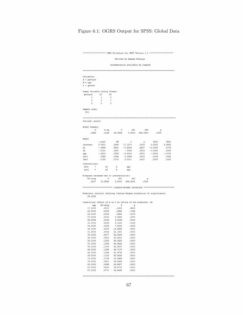
Figure 6.1: OGRS Output for SPSS: Global Data

67

Figure 6.2: OGRS Output for SAS: Global Data

68

Figure 6.3: Graph of Predicted Support for Government Action across Party Identi-fication and Age

.03, p < .001), means that the difference between Republicans and Democrats in

support for government action against climate change is expected to change as age

changes. Specifically, as age increases by one year the difference between Democrats

and Republicans is estimated to increase by .03 units, where democrats are estimated

to be more supportive of government action relative to Republicans as age increases.

This can be seen clearly in Figure 6.3, as age increases support for government action

increases among Democrats, and decreases among Republicans.

Similarly, the coefficient for D2M (b = .0155, p = .0427), means that the difference

between Republicans and Independents in support for government action against cli-

mate change is also estimated to increase as age increases. As age increases by one

69

year, the difference between Independents and Republicans is estimated to increase

by .02 units, where independents are estimated to be more supportive of government

action relative to Republicans as age increases. Based on Figure 2 it seems that

Independents support decreases slightly as age increases, but the decrease for Repub-

licans is stronger, and the gap between Independents and Republicans increases as

age increases.

Based on the regression coefficients, it seems that there is a clear interaction

between party identification and age in predicting support of government actions.

However, there are many instances where one product coefficient is significant and

the other is not, or both are marginally significant. In these cases, and in all cases,

it is best to examine a formal test of whether allowing the relationship between

the independent variable and the outcome to depend on the moderator increases the

explained variance in the outcome variable. This test is provided at the bottom of the

second section of the OGRS output labeled “R-square increase due to interaction(s)”.

This is the test comparing the model without either of the product coefficients, and

thus fixing the effect of political identification on support of government action to be

constant across age, to the model which allows this effect to vary across age. Based

on the output allowing this relationship to vary across age explains an estimated

additional 2% of the variance in support in government actions (F (2, 809) = 10.39,

p < .001). This provides clear support for the hypothesis that the effect of political

party on support for government action to mitigate climate change depends on age

of respondents.

Based on this finding it would be reasonable to wonder “At what point does

political party matter?” Alternatively, at what ages are there significant differences

70

between political parties on support for government action against climate change?

This is a question which can be answered by using the Johnson-Neyman procedure

for categorical independent variables. In the third section of the OGRS output labeled

Johnson-Neyman Technique, there is output from the iterative program described

in the previous chapter. The age at which the differences between political parties

transitions from being significant to non-significant is 29.33 years. Based on the table

below the Johnson-Neyman solutions, individuals below the age of 29.33 show no

significant party divides on support for government action, but for individuals above

the age of 29.33, party identification has a significant effect on support for government

action against climate change. By defining regions of significance and regions of non-

significance, the Johnson-Neyman procedure eliminates the need to probe at a variety

of arbitrary points along the moderator. Instead based on these regions we know if

the effect of party identification is significant for any point based on which of these

regions it is contained in.

71

Chapter 7: Discussion

An approximate method for finding Johnson-Neyman boundaries of significance

in an omnibus test of group difference should provide opportunities for researchers

to answer new questions. Particularly in psychology, researchers often care about

categorical variables such as ethnicity, and it is important that researchers have the

ability to estimate moderation effects and probe them using the most sophisticated

methods available. I began this thesis by explaining common methods of estimating

and probing interaction effects in linear regression. I overviewed the history of the

development of the Johnson-Neyman procedure, in order to show how the procedure

has grown from use just in an ANCOVA to any linear regression. Using the principles

of the Johnson-Neyman procedure in linear regression and the general linear model,

I derived the boundaries of significance for a three category variable. Using the same

method, I showed why the closed form derivation of the Johnson-Neyman boundaries

of significance is not possible for more than four groups. I developed an iterative

tool which can approximate these boundaries. I have shown that the tool achives

very close solutions when the solutions are known and runs in a reasonable amount

of time. I then showed how the tool is used and how the output is interpreted with

a real data example about party differences in support for government action against

global warming.

72

7.1 Uses and Non-Uses

My hope is that this tool will help researchers answer questions that they previ-

ously could not answer. There are many instances where other types of analyses are

more appropriate for a question, and my aim is not for people to use this method

in lieu of other more appropriate methods, but rather to use this method when it is

most relevant to the question at hand. Many researchers with categorical variables

are most interested in pairwise comparisons For example, when a researcher runs an

experiment with two control conditions and an experimental condition, this may be

an instance where the researcher is not particularly interested in omnibus group dif-

ferences, and in this case the researcher could use the Johnson-Neyman procedures

developed for pairwise comparisons. However, there are many instances where om-

nibus group differences are most relevant to a researcher’s question of interest, and in

that case I recommend using this tool over others where only the results for pairwise

comparisons are available.

7.2 Future Directions

There are many extensions of this Johnson-Neyman approximation which may

be of use to researchers. For example, allowing for multiple moderators may help

researchers identify more complex regions of significance which are of higher dimen-

sion. With one moderator, there is only one dimension which needs to be searched,

but with j moderators, there would be a j dimensional surface which would need to

be searched for Johnson-Neyman transition points. In this situation the boundary of

significance is a function, rather than a few points. This problem is complicated in

two ways. First, developing a search algorithm to thoroughly search multidimensional

73

spaces is more difficult than the current one dimensional problem dealt with in this

thesis. Second, there will be infinite transition points, and thus the goal might be to

define a function which describes this transition point. The form of such a function is

known in the continuous and dichotomous independent variable case (Abelson, 1953),

but in the categorical independent variable case it is currently unknown.

Moderation can take many forms. Throughout this thesis I have dealt solely with

linear moderation, where the effect of X on Y is a linear function of M . Other

forms of moderation, like higher level polynomial functions, would require defining

a different contrast matrix L. If the corresponding contrast matrix results in F

being a polynomial function of M of any order, then the methods here could be

applied to other types of moderation. However, not all contrast matrices will result

in a polynomial function of M , and so the method proposed in this thesis is not

generalizable to all types of moderation, but could potentially be generalized to other

certain kinds of moderation.

Hayes and Matthes (2009) generalized the Johnson-Neyman procedure to linear

regression with a dichotomous outcome. In principle, this could be done with the

current method as well. Because logistic regression requires a maximum likelihood

algorithm to estimate the coefficients and significance tests, and the Johnson-Neyman

approximation proposed in this thesis requires iterative estimation of these models,

program run time could become unreasonably long. A more efficient search algorithm

could be used in combination with logistic regression to generalize this procedure to

dichotomous outcomes.

Researchers are often interested in where along the range of a moderator the inde-

pendent variable no longer has an effect (e.g., Voorhees, Baker, Bourdeau, Brocato,

74

& Cronin Jr., 2009), for whom some intervention would be effective (e.g., Oyser-

man, Brickman, & Rhodes, 2007), or who that may be particularly at risk for some

outcome(e.g., Hilmer et al., 2008). One major misconception of the Johnson-Neyman

procedure is that the boundaries of significance are good estimates of these points.

Some researchers even make recommendations for treatments and decisions based on

the findings of the Johnson-Neyman procedure. Other researchers have even com-

pared transition points from one study to another, suggesting that the results are

contradictory because the transition points were different (Carlson & Iacono, 2008).

Because the boundaries of significance identify where an effect is statistically signifi-

cant, they will be very dependent on study elements like sample size and effect size or

strength of manipulation. Certain researchers may benefit from having an estimate of

the point where an effect is zero, or the smallest it gets. These would not necessarily

be the Johnson-Neyman boundaries of significance. The boundaries of significance

will approach the point(s) along the moderator where the independent variable no

longer has an effect as sample size increases. However, at any sample size, there is a

better estimate of this point, which is the sample estimate of where the effect is zero.

When there are two groups, a good estimate of when an effect is zero is the estimate

of where the two groups have the same expected value on the outcome. For example,

if X is a dichotomous variable coded 0 and 1, and the regression model is:

E(Yi) = b0 + b1Xi + b2Mi + b3XiMi.

Then the expected value of Y when X is 0 is

E(Yi|X = 0) = b0 + b2Mi,

75

and the expected value of Y when X is 1 is

E(Yi|X = 0) = b0 + b1 + b2Mi + b3Mi.

By setting these two equations equal to each other, and solving for M, this gives an

estimate of M such that the effect of X is zero.

b0 + b2Mi = b0 + b1 + b2Mi + b3Mi

0 = b1 + b3Mi

b1/b3 = M

This would be a better estimate of the point where the effect of X on Y is zero. The

sampling distribution of this point likely has an unusual shape, as the distribution of

the quotient of two normally distributed variables is not neccesarily normal. Methods

such as bootstrapping could be used to provide a confidence interval for this point.

Generalizing this method to categorical independent variables could be more complex,

as there may be no point along the moderator where the effect of X is estimated to

be zero. In this case, it could be worthwhile to estimate the point where the effect of

the independent variable on the outcome is smallest instead. Some investigation into

this estimate and elaboration on how the Johnson-Neyman points are sample-size

dependent and are not a good estimate of when an independent variable has no effect

could be useful in ensuring appropriate use of the Johnson-Neyman procedure.

7.3 Conclusion

The Johnson-Neyman procedure has been continuously generalized to more and

more situations since it’s development. I believe this is because it is a useful statis-

tical tool that helps researchers better understand and visualize interactions, which

76

can often be very complicated. My original goal in this thesis was to provide an ana-

lytical solution to the Johnson-Neyman boundaries of significance with a categorical

independent variable with any number of groups. Through my investigation of this

topic I discovered that a true analytical solution would not be possible; however, I

developed an iterative computer program which provides good approximations to the

Johnson-Neyman boundaries under the conditions tested in this thesis, and I believe

this tool could be helpful to researchers investigating questions of moderation of the

effect of a categorical independent variable on some outcome.

77

References

Abamowitz, M., & Stegun, I. A. (1964). Handbook of mathematical functions withformulas, graphs, and mathematical tables. Washington D. C.: Dover Publica-tions.

Abel, N. H. (1824). Memoire sur les equations algebriques: ou on demontrel’impossibilite de la resolution de l’equation generale du cinquieme degre. Groen-dahl: Christiana.

Abelson, R. P. (1953). A note on the Neyman-Johnson technique. Psychometrika,18 (3), 213–218.

Aiken, L. S., & West, S. G. (1991). Multiple regression: Testing and interpretinginteractions. Thousand Oaks, CA: Sage.

Barajas-Gonzales, R. G., & Brooks-Gunn, J. (2014). Income, neighborhood stressors,and harsh parenting: Test of moderation by ethnicity, age, and gender. Journalof Family Psychology , 28 (6), 855–866.

Bauer, D. J., & Curran, P. J. (2005). Probing interactions in fixed and multilevelregression: Inferential and graphical techniques. Multivariate Behavioral Re-search, 40 (3), 373–400.

Bratley, P., Fox, B. L., & Schrage, L. E. (1983). A guide to simulation. New York:Springer-Verlag.

Campbell, N. J. (1990). High school students computer attitudes and attributions:Gender and ethnic group differences. Journal of Adolescent Research, 5 (4),485–499.

Carlson, S. R., & Iacono, W. G. (2008). Deviant P300 amplitude developmentin males is associated with paternal exteralizing psychopathology. Journal ofAbnormal Psychology , 117 (4), 910–923.

Carroll, J. B., & Wilson, G. F. (1970). An interactive-computer program for theJohnson-Neyman technique in the case of two-groups, two predictor variables,and one criterion variable. Educational and Psychological Measurement , 30 ,121–132.

Cleveland, M. J., Hultgren, B., Varvil-Weld, L., Mallett, K. A., Turrisi, R., & Abar,C. C. (2013). Moderation of a parent-based intervention on transitions in drink-ing: Examining the role of normative perceptions and attitudes among high-and low-risk first-year college students. Alcoholism: Clinical and ExperimentalResearch, 37 (9), 1587–1594.

78

Cohen, J., Cohen, P., West, S. G., & Aiken, L. S. (2003). Applied multiple regres-sion/correlation analysis for the behavioral sciences (3rd ed.). Mahwah, NJ:Erlbaum.

D’Alonzo, K. T. (2004). The Johnson-Neyman procedure as an alternative to AN-COVA. Western Journal of Nursing Research, 26 (7), 804–812.

Darlington, R. B., & Hayes, A. F. (2017). Regression analysis and linear models: Con-cepts, applications, and implementation. New York, New York: The GuilfordPress.

DeRemer, M. (1989). The computer gender gap in elementary school. Computers inthe Schools , 6 (3–4), 39–50.

Engqvist, L. (2005). The mistreatment of covariate interaction terms in linear modelanalyses of behavioural and evolutionary ecology studies. Animal Behavior , 70 ,967–971.

Field, A. (2013). Discovering Statistics using IBM SPSS Statistics (4th ed.). Thou-sand Oaks, CA: Sage.

Forster, F. (1971). The generalized Johnson-Neyman procedures: An approach tocovariate adjustment and interaction analysis. Paper presented at the AnnualMeeting of the American Educational Research Association, New York, NY.

Forster, F. (1974). An alternative to ANCOVA when group regressions are heteroge-nous: The generalized Johnson-Neyman procedure. Paper presented at the An-nual Meeting of the American Educational Research Association, Washington,D. C.

Greenberg, M., & Truelove, M. B. (2011). Energy choices and risk beliefs: Is it justglobal warming and a fear of a nuclear power plant accident? Risk Analysis ,31 (5), 819–831.

Guber, D. L. (2013). A cooling climate for change? Party polarization and thepolitics of global warming. American Behavioral Scientist , 57 (1), 93–115.

Hayes, A. F. (2013). Introduction to mediation, moderation, and conditional processanalysis. New York, NY: Guilford Press.

Hayes, A. F., & Matthes, J. (2009). Computational procedures for probing interac-tions in OLS and logistic regression: SPSS and SAS implementations. BehaviorResearch Methods , 41 (3), 924–936.

Hilmer, C. J., Schetter, C. D., Dominguez, T. P., Abdou, C., Hobel, C. J., Glynn,L., & Sandman, C. (2008). Stress and blood pressure during pregnancy: Racialdifferences and associations with birthweight. Psychosomatic Medicine, 70 ,57–64.

Hoffman, L. (2011). Talking past each other? Cultural framing of skeptical andconvinced logics in the climate change debate. Organization & Environment ,24 (1), 3–33.

Howell, D. C. (2007). Statistical methods for psychology. Belmont, CA: ThomsonWadsworth.

Huitema, B. E. (1980). The analysis of covariance and alternatives. New York, NY:John Wiley.

79

Hunka, S. (1995). Identifying region of significance in ANCOVA problems havingnon-homogenous regressions. British Journal of Mathematical and StatisticalPsychology , 48 , 161–188.

Hunka, S., & Leighton, J. (1997). Defining Jjohnson-Neyman regions of signifiance inthe three-covariate ANCOVA using Mathematica. Journal of Educational andBehavioral Statistics , 22 (4), 361–387.

Jaccard, J., & Turrisi, R. (2003). Interaction effects in multiple regression (2nd ed.).Thousand Oaks, CA: Sage.

Johnson, P. O., & Fay, L. F. (1950). The Johnson-Neyman technique, its theory andapplication. Psychometrika, 15 (4), 349–367.

Johnson, P. O., & Hoyt, C. (1947). On determining three dimensional regions ofsignificance. Journal of Experimental Education, 15 , 203–212.

Johnson, P. O., & Neyman, J. (1936). Tests of certain linear hypotheses and theirapplication to some educational problems. Statistical Research Memoirs , 1 ,57–93.

Joslyn, S. L., & LeClerc, J. E. (2016). Climate projections and uncertainty commu-nication. Topics in Cognitive Science, 8 , 222–241.

Karpman, M. B. (1983). The Johnson-Neyman technique using SPSS or BMDP.Educational and Psychological Measurement , 43 , 137–147.

Karpman, M. B. (1986). Comparing two non-parallel regression lines with the para-metric alternative to analysis of covariance using SPSS-X or SAS – The Johnson-Neyman Technique. Educational and Psychological Measurement , 46 , 639–644.

Kim, Y., & Baek, Y. M. (2014). When is selective self-presentation effective? Aninvestigation of the moderation effect of “self-esteem” and “social trust”. Cy-berpsychology, Behavior, and Social Networking , 17 (11), 697–701.

McCright, A. M., & Dunlap, R. E. (2011). The politicization of climate changeand polization in the American public’s view of global warming, 2001–2010.Sociological Quarterly , 52 (2), 155–194.

Niederdeppe, J., Shapiro, M. A., Kim, H. K., Bartolo, D., & Porticella, N. (2014).Narrative persuasion, causality, complex integration, and support for obesitypolicy. Health Communications , 29 , 431–444.

Nisbet, M. C., & Myers, T. (2007). The polls-trend: Twenty years of public opinionabout global warming. Public Opinion Quarterly , 71 (3), 444–470.

O’Connor, B. P. (1998). SIMPLE: All-in-one programs for exploring interactionsin moderated multiple regression. Educational and Psychological Measurement ,58 (5), 836–840.

O’Malley, M., Voight, A., Renshaw, T. L., & Eklund, K. (2015). School climate,family structure, and academic achievement: A study of moderation effects.School Psychology Quarterly , 30 (1), 142–157.

Oyserman, D., Brickman, D., & Rhodes, M. (2007). School success, possible selves,and parent school involvement. Family Relations , 56 , 479–489.

Pedhazur, E. J. (1997). Multiple regression in behavioral research (3rd ed.). Orlando,FL: Harcourt Brace.

80

Potthoff, R. F. (1964). On the Johnson-Neyman technique and some extensionsthereof. Psychometrika, 29 (3), 241–256.

Preacher, K. J., Curran, P. J., & Bauer, D. J. (2006). Computational tools for probinginteractions in multiple linear regression, multilevel modeling, and latent curveanalysis. Journal of Educational & Behavioral Statistics , 31 (3), 437–488.

Roots [Computer program manual]. (n.d.). Wolfram Lanugage & System Documenta-tion Center. Retrieved January 2016, from https://reference.wolfram.com/

language/ref/Roots.html

Ruffini, P. (1799). Teoria general delle equazioni, in cui si dimonstra impossi-bile la soluzione albegraica delle equazioni generali de grado superior al quarto.Bologna, Italy: Nella stamperia di S. T. d’Aquino.

Schuldt, J. P., Roh, S., & Schwarz, N. (2015). Questionnaire design effects in cli-mate change surveys: Implications for the partisan divide. The Annals of theAmerican Academy of Political and Social Science, 658 , 67–85.

Siy, J. O., & Cheryan, S. (2013). When compliments fail to flatter: Americanindividualism and responses to positive stereotypes. Johnson of Personalityand Social Psychology , 104 (1), 87–102.

Spiller, S. A., Fitzimons, G. J., Lynch Jr., J. G., & McClelland, G. H. (2013). Spot-lights, floodlights, and the magic number zero: Simple effects tests in moderatedregression. Journal of Marketing Research, 50 , 277–288.

Voorhees, C. M., Baker, J., Bourdeau, B. L., Brocato, E. D., & Cronin Jr., J. J. (2009).It depends: Moderating the relationships among perceived waiting time, anger,and regret. Journal of Service Research, 12 (2), 138–155.

Whitley Jr., B. E. (1997). Gender differences in computer-related attitudes andbehavior: A meta-analysis. Computers in Human Behavior , 13 (1), 1–22.

81

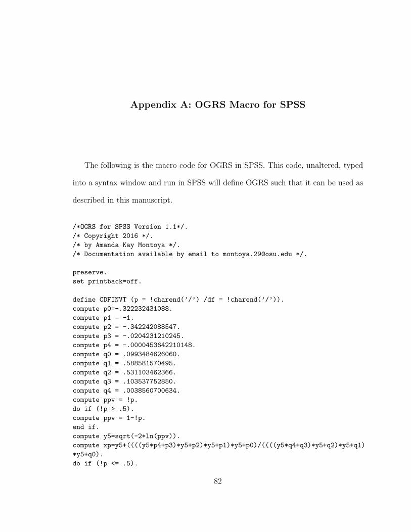
Appendix A: OGRS Macro for SPSS

The following is the macro code for OGRS in SPSS. This code, unaltered, typed

into a syntax window and run in SPSS will define OGRS such that it can be used as

described in this manuscript.

/*OGRS for SPSS Version 1.1*/.

/* Copyright 2016 */.

/* by Amanda Kay Montoya */.

/* Documentation available by email to montoya.29@osu.edu */.

preserve.

set printback=off.

define CDFINVT (p = !charend(’/’) /df = !charend(’/’)).

compute p0=-.322232431088.

compute p1 = -1.

compute p2 = -.342242088547.

compute p3 = -.0204231210245.

compute p4 = -.0000453642210148.

compute q0 = .0993484626060.

compute q1 = .588581570495.

compute q2 = .531103462366.

compute q3 = .103537752850.

compute q4 = .0038560700634.

compute ppv = !p.

do if (!p > .5).

compute ppv = 1-!p.

end if.

compute y5=sqrt(-2*ln(ppv)).

compute xp=y5+((((y5*p4+p3)*y5+p2)*y5+p1)*y5+p0)/((((y5*q4+q3)*y5+q2)*y5+q1)

*y5+q0).

do if (!p <= .5).

82

compute xp = -xp.

end if.

compute toutput = sqrt(!df*(exp((!df-(5/6))*(xp**2)/(!df-(2/3)+.1/!df)**2)

-1)).

!enddefine.

define CORR (var1 = !charend(’/’) /var2 = !charend(’/’)).

COMPUTE var1 = !var1.

COMPUTE var2 = !var2.

COMPUTE MeanV1 = csum(var1)/nrow(var1).

COMPUTE MeanV2 = csum(var2)/nrow(var2).

COMPUTE Var1Cent = var1 - MeanV1.

COMPUTE Var2Cent = var2 - MeanV2.

COMPUTE crosprod = csum(Var1Cent &* Var2Cent).

COMPUTE Var1SS = csum(Var1Cent &* Var1Cent).

COMPUTE Var2SS = csum(Var2Cent &* Var2Cent).

COMPUTE rPears = crosprod / (sqrt(var1SS)*sqrt(var2SS)).

!enddefine.

define RedR (center = !charend(’/’)).

COMPUTE mcent = m - !center.

COMPUTE m2int = MAKE(N, numgroup-1, -999).

LOOP i4 = 1 to (numgroup-1).

COMPUTE m2int(:,i4) = mcent&*data(:,i4+1).

END LOOP.

COMPUTE datam2 = {MAKE(N,1,1), mcent, m2int}.

DO IF covtog = 1.

COMPUTE datam2 = {datam2, data(:,(2*numgroup+1):ncol(data))}.

END IF.

COMPUTE yestm2 = datam2*inv(t(datam2)*datam2)*t(datam2)*y.

CORR var1 = y /var2 = yestm2.

COMPUTE ycorm2 = rPears.

COMPUTE redr2 = ycorm2**2.

!enddefine.

define PROBE (min = !charend(’/’) /max = !charend(’/’)).

COMPUTE jump = (!max - !min)/iter.

COMPUTE dim = (transtog=0)*(iter+1) + (transtog=1)*(iter-1).

COMPUTE tempres = MAKE(dim, 8, -999).

DO IF transtog = 0.

COMPUTE i2 = !min.

ELSE IF transtog = 1.

COMPUTE i2 = !min+jump.

END IF.

LOOP i = 1 to dim.

83

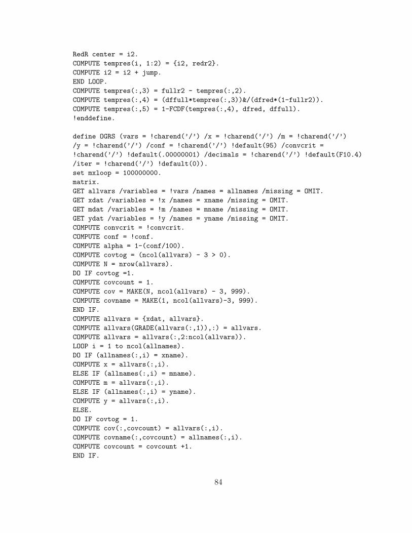
RedR center = i2.

COMPUTE tempres(i, 1:2) = {i2, redr2}.

COMPUTE i2 = i2 + jump.

END LOOP.

COMPUTE tempres(:,3) = fullr2 - tempres(:,2).

COMPUTE tempres(:,4) = (dffull*tempres(:,3))&/(dfred*(1-fullr2)).

COMPUTE tempres(:,5) = 1-FCDF(tempres(:,4), dfred, dffull).

!enddefine.

define OGRS (vars = !charend(’/’) /x = !charend(’/’) /m = !charend(’/’)

/y = !charend(’/’) /conf = !charend(’/’) !default(95) /convcrit =

!charend(’/’) !default(.00000001) /decimals = !charend(’/’) !default(F10.4)

/iter = !charend(’/’) !default(0)).

set mxloop = 100000000.

matrix.

GET allvars /variables = !vars /names = allnames /missing = OMIT.

GET xdat /variables = !x /names = xname /missing = OMIT.

GET mdat /variables = !m /names = mname /missing = OMIT.

GET ydat /variables = !y /names = yname /missing = OMIT.

COMPUTE convcrit = !convcrit.

COMPUTE conf = !conf.

COMPUTE alpha = 1-(conf/100).

COMPUTE covtog = (ncol(allvars) - 3 > 0).

COMPUTE N = nrow(allvars).

DO IF covtog =1.

COMPUTE covcount = 1.

COMPUTE cov = MAKE(N, ncol(allvars) - 3, 999).

COMPUTE covname = MAKE(1, ncol(allvars)-3, 999).

END IF.

COMPUTE allvars = {xdat, allvars}.

COMPUTE allvars(GRADE(allvars(:,1)),:) = allvars.

COMPUTE allvars = allvars(:,2:ncol(allvars)).

LOOP i = 1 to ncol(allnames).

DO IF (allnames(:,i) = xname).

COMPUTE x = allvars(:,i).

ELSE IF (allnames(:,i) = mname).

COMPUTE m = allvars(:,i).

ELSE IF (allnames(:,i) = yname).

COMPUTE y = allvars(:,i).

ELSE.

DO IF covtog = 1.

COMPUTE cov(:,covcount) = allvars(:,i).

COMPUTE covname(:,covcount) = allnames(:,i).

COMPUTE covcount = covcount +1.

END IF.

84

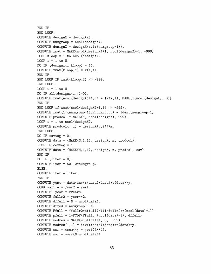
END IF.

END LOOP.

COMPUTE designX = design(x).

COMPUTE numgroup = ncol(designX).

COMPUTE designX = designX(:,1:(numgroup-1)).

COMPUTE xmat = MAKE(ncol(designX)+1, ncol(designX)+1, -999).

LOOP kloop = 1 to ncol(designX).

LOOP i = 1 to N.

DO IF (designx(i,kloop) = 1).

COMPUTE xmat(kloop,1) = x(i,1).

END IF.

END LOOP IF xmat(kloop,1) <> -999.

END LOOP.

LOOP i = 1 to N.

DO IF all(designx(i,:)=0).

COMPUTE xmat(ncol(designX)+1,:) = {x(i,1), MAKE(1,ncol(designX), 0)}.

END IF.

END LOOP if xmat(ncol(designX)+1,1) <> -999).

COMPUTE xmat(1:(numgroup-1),2:numgroup) = Ident(numgroup-1).

COMPUTE prodcol = MAKE(N, ncol(designX), 999).

LOOP i = 1 to ncol(designX).

COMPUTE prodcol(:,i) = designX(:,i)&*m.

END LOOP.

DO IF covtog = 0.

COMPUTE data = {MAKE(N,1,1), designX, m, prodcol}.

ELSE IF covtog = 1.

COMPUTE data = {MAKE(N,1,1), designX, m, prodcol, cov}.

END IF.

DO IF (!iter = 0).

COMPUTE iter = 50+10*numgroup.

ELSE.

COMPUTE iter = !iter.

END IF.

COMPUTE yest = data*inv(t(data)*data)*t(data)*y.

CORR var1 = y /var2 = yest.

COMPUTE ycor = rPears.

COMPUTE fullr2 = ycor**2.

COMPUTE dffull = N - ncol(data).

COMPUTE dfred = numgroup - 1.

COMPUTE Ffull = (fullr2*dffull)/((1-fullr2)*(ncol(data)-1)).

COMPUTE pfull = 1-FCDF(Ffull, (ncol(data)-1), dffull).

COMPUTE modres = MAKE(ncol(data), 6, -999).

COMPUTE modres(:,1) = inv(t(data)*data)*t(data)*y.

COMPUTE ssr = csum((y - yest)&**2).

COMPUTE msr = ssr/(N-ncol(data)).

85

COMPUTE semat = (msr*inv(t(data)*data)).

COMPUTE modres(:,2) = (diag(semat))&**(1/2).

COMPUTE modres(:,3) = modres(:,1)&/modres(:,2).

COMPUTE modres(:,4) = 2*(1-tcdf(abs(modres(:,3)),dffull)).

COMPUTE temp = alpha/2.

CDFINVT p = temp /df = dffull.

COMPUTE tcrit = toutput.

COMPUTE modres(:,5) = modres(:,1) - tcrit*modres(:,2).

COMPUTE modres(:,6) = modres(:,1) + tcrit*modres(:,2).

DO IF covtog = 0.

COMPUTE dataint = {MAKE(N,1,1), designX, m}.

ELSE IF covtog = 1.

COMPUTE dataint = {MAKE(N,1,1), designX, m, cov}.

END IF.

COMPUTE yestint = dataint*inv(t(dataint)*dataint)*t(dataint)*y.

CORR var1 = y /var2 = yestint.

COMPUTE ycorint = rPears.

COMPUTE r2int = ycorint**2.

COMPUTE rchint = fullr2 - r2int.

COMPUTE Fint = (dffull*rchint)&/(dfred*(1-fullr2)).

COMPUTE pint = 1-FCDF(Fint, dfred, dffull).

COMPUTE intres = {rchint, Fint, dfred, dffull, pint}.

COMPUTE transtog = 0.

COMPUTE minM = cmin(m).

COMPUTE maxM = cmax(m).

PROBE min = minM /max = maxM.

COMPUTE results = tempres.

COMPUTE OGres = tempres.

COMPUTE results(nrow(results),6:7) = {0,0}.

COMPUTE i3 = 1.

LOOP IF i3 <= nrow(results).

DO IF i3 < nrow(results).

COMPUTE results(i3, 6) = 1*(results(i3,4) < results(i3+1,4)) -

1*(results(i3,4) > results(i3+1,4)).

COMPUTE results(i3, 7) = -1*((results(i3,5) < alpha) AND

(results(i3+1,5) > alpha)) + 1*((results(i3,5) > alpha) AND

(results(i3+1, 5) < alpha)).

END IF.

COMPUTE results(i3,8) = (abs(results(i3,5) - alpha) < convcrit).

DO IF i3 = nrow(results).

COMPUTE transcnv = 0.

ELSE IF i3 = 1.

COMPUTE transcnv = ((results(i3,7) = 1)AND((results(i3,8)=1)OR

(abs(results(i3+1,5) - alpha) < convcrit))).

ELSE.

86

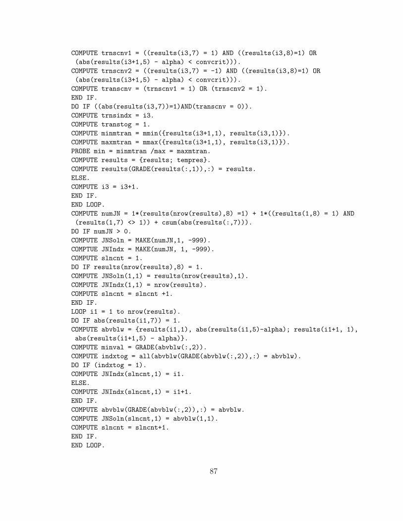
COMPUTE trnscnv1 = ((results(i3,7) = 1) AND ((results(i3,8)=1) OR

(abs(results(i3+1,5) - alpha) < convcrit))).

COMPUTE trnscnv2 = ((results(i3,7) = -1) AND ((results(i3,8)=1) OR

(abs(results(i3+1,5) - alpha) < convcrit))).

COMPUTE transcnv = (trnscnv1 = 1) OR (trnscnv2 = 1).

END IF.

DO IF ((abs(results(i3,7))=1)AND(transcnv = 0)).

COMPUTE trnsindx = i3.

COMPUTE transtog = 1.

COMPUTE minmtran = mmin({results(i3+1,1), results(i3,1)}).

COMPUTE maxmtran = mmax({results(i3+1,1), results(i3,1)}).

PROBE min = minmtran /max = maxmtran.

COMPUTE results = {results; tempres}.

COMPUTE results(GRADE(results(:,1)),:) = results.

ELSE.

COMPUTE i3 = i3+1.

END IF.

END LOOP.

COMPUTE numJN = 1*(results(nrow(results),8) =1) + 1*((results(1,8) = 1) AND

(results(1,7) <> 1)) + csum(abs(results(:,7))).

DO IF numJN > 0.

COMPUTE JNSoln = MAKE(numJN,1, -999).

COMPTUE JNIndx = MAKE(numJN, 1, -999).

COMPUTE slncnt = 1.

DO IF results(nrow(results),8) = 1.

COMPUTE JNSoln(1,1) = results(nrow(results),1).

COMPUTE JNIndx(1,1) = nrow(results).

COMPUTE slncnt = slncnt +1.

END IF.

LOOP i1 = 1 to nrow(results).

DO IF abs(results(i1,7)) = 1.

COMPUTE abvblw = {results(i1,1), abs(results(i1,5)-alpha); results(i1+1, 1),

abs(results(i1+1,5) - alpha)}.

COMPUTE minval = GRADE(abvblw(:,2)).

COMPUTE indxtog = all(abvblw(GRADE(abvblw(:,2)),:) = abvblw).

DO IF (indxtog = 1).

COMPUTE JNIndx(slncnt,1) = i1.

ELSE.

COMPUTE JNIndx(slncnt,1) = i1+1.

END IF.

COMPUTE abvblw(GRADE(abvblw(:,2)),:) = abvblw.

COMPUTE JNSoln(slncnt,1) = abvblw(1,1).

COMPUTE slncnt = slncnt+1.

END IF.

END LOOP.

87

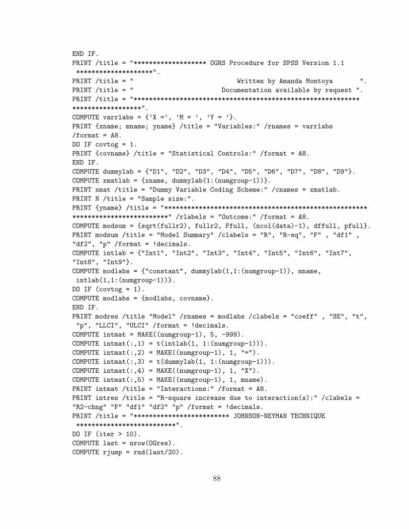
END IF.

PRINT /title = "******************* OGRS Procedure for SPSS Version 1.1

********************".

PRINT /title = " Written by Amanda Montoya ".

PRINT /title = " Documentation available by request ".

PRINT /title = "***********************************************************

******************".

COMPUTE varrlabs = {’X =’, ’M = ’, ’Y = ’}.

PRINT {xname; mname; yname} /title = "Variables:" /rnames = varrlabs

/format = A8.

DO IF covtog = 1.

PRINT {covname} /title = "Statistical Controls:" /format = A8.

END IF.

COMPUTE dummylab = {"D1", "D2", "D3", "D4", "D5", "D6", "D7", "D8", "D9"}.

COMPUTE xmatlab = {xname, dummylab(1:(numgroup-1))}.

PRINT xmat /title = "Dummy Variable Coding Scheme:" /cnames = xmatlab.

PRINT N /title = "Sample size:".

PRINT {yname} /title = "*****************************************************

*************************" /rlabels = "Outcome:" /format = A8.

COMPUTE modsum = {sqrt(fullr2), fullr2, Ffull, (ncol(data)-1), dffull, pfull}.

PRINT modsum /title = "Model Summary" /clabels = "R", "R-sq", "F" , "df1" ,

"df2", "p" /format = !decimals.

COMPUTE intlab = {"Int1", "Int2", "Int3", "Int4", "Int5", "Int6", "Int7",

"Int8", "Int9"}.

COMPUTE modlabs = {"constant", dummylab(1,1:(numgroup-1)), mname,

intlab(1,1:(numgroup-1))}.

DO IF (covtog = 1).

COMPUTE modlabs = {modlabs, covname}.

END IF.

PRINT modres /title "Model" /rnames = modlabs /clabels = "coeff" , "SE", "t",

"p", "LLCI", "ULCI" /format = !decimals.

COMPUTE intmat = MAKE((numgroup-1), 5, -999).

COMPUTE intmat(:,1) = t(intlab(1, 1:(numgroup-1))).

COMPUTE intmat(:,2) = MAKE((numgroup-1), 1, "=").

COMPUTE intmat(:,3) = t(dummylab(1, 1:(numgroup-1))).

COMPUTE intmat(:,4) = MAKE((numgroup-1), 1, "X").

COMPUTE intmat(:,5) = MAKE((numgroup-1), 1, mname).

PRINT intmat /title = "Interactions:" /format = A8.

PRINT intres /title = "R-square increase due to interaction(s):" /clabels =

"R2-chng" "F" "df1" "df2" "p" /format = !decimals.

PRINT /title = "************************* JOHNSON-NEYMAN TECHNIQUE

**************************".

DO IF (iter > 10).

COMPUTE last = nrow(OGres).

COMPUTE rjump = rnd(last/20).

88

COMPTUE rowsel = 1.

COMPUTE rcount = 1+rjump.

LOOP IF (rcount <= last).

COMPUTE rowsel = {rowsel, rcount}.

COMPUTE rcount = rcount + rjump.

END LOOP.

DO IF (rcount - rjump <> last).

COMPUTE rowsel = {rowsel, last}.

END IF.

END IF.

COMPUTE JNtabnam = {mname, "R2-chng", "F", "p"}.

DO IF numJN > 0.

PRINT JNSoln /title = "Moderator value(s) defining Johnson-Neyman boundaries

of significance:" /format = !decimals.

DO IF (iter > 10).

COMPUTE JNouttab = {OGres(rowsel,:); results(JNIndx, :)}.

ELSE.

COMPUTE JNouttab = {OGres(:,:);results(JNIndx,:)}.

END IF.

COMPUTE JNouttab(GRADE(JNouttab(:,1)),:) = JNouttab.

COMPUTE JNouttab = JNouttab(:,{1,3,4,5}).

PRINT JNouttab /title = "Conditional effect of X on Y at values of the

moderator (M)" /cnames = JNtabnam /format = !decimals.

ELSE.

PRINT /title = "No Johnson-Neyman bounds found within range of observed

data".

DO IF (iter > 10).

COMPUTE JNouttab = OGres(rowsel,{1,3,4,5}).

ELSE.

COMPUTE JNouttab = OGres(:,{1,3,4,5}).

END IF.

PRINT JNouttab /title = "Conditional effect of X on Y at values of the

moderator (M)" /cnames = JNtabnam /format = !decimals.

END IF.

PRINT /title = "********************************************************

*********************".

end matrix.

!enddefine.

restore.

89

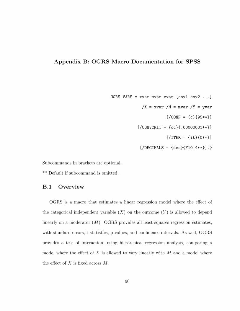
Appendix B: OGRS Macro Documentation for SPSS

OGRS VARS = xvar mvar yvar [cov1 cov2 ...]

/X = xvar /M = mvar /Y = yvar

[/CONF = {c}{95**}]

[/CONVCRIT = {cc}{.00000001**}]

[/ITER = {it}{0**}]

[/DECIMALS = {dec}{F10.4**}].}

Subcommands in brackets are optional.

** Default if subcommand is omitted.

B.1 Overview

OGRS is a macro that estimates a linear regression model where the effect of

the categorical independent variable (X) on the outcome (Y ) is allowed to depend

linearly on a moderator (M). OGRS provides all least squares regression estimates,

with standard errors, t-statistics, p-values, and confidence intervals. As well, OGRS

provides a test of interaction, using hierarchical regression analysis, comparing a

model where the effect of X is allowed to vary linearly with M and a model where

the effect of X is fixed across M .

90

OGRS also provides a unique method for probing the effect of X on Y using

an approximation of the Johnson-Neyman procedure. OGRS searches the observed

range of the moderator for points at which the effect of X on Y transitions from

significant to non-significant or vice versa, as specified by some level of confidence

(CONF). OGRS prints the transition points if any exist within the observed range of

the moderator, as well as a table of points along the moderator, statistics related to

the estimated effect of X at that point, and inferential statistics for the effect of X.

B.2 Preparation for Use

The OGRS.sps file should be opened as a syntax file in SPSS. Once opened,

execute the entire file exactly as is. Do not modify the code. Once the program

is executed, the OGRS.sps file window can be closed. Once executed, access to the

OGRS command is available until quitting SPSS. The OGRS.sps file must be loaded

and re-executed each time SPSS is opened.

B.3 Model Specification

Because OGRS will only accept one variable in the X subcommand, your inde-

pendent variable should be coded into one variable, with unique codes for each group.

Categorical independent variables can represent groups (e.g. race, political party),

experimental conditions, or any other categorical variable of interest. Both the mod-

erator M and the outcome variable Y are treated as continuous variables. Covariates

specified in the model can be continuous or dichotomous, but they cannot be cate-

gorical with more than two groups. To use categorical covariates, using your desired

coding scheme (e.g. dummy coding) to create k − 1 new variables to represent your

91

categorical covariate, and include all of these variables as covariates in the model.

Covariates can be included in the vars subcommand, and they will be included in

the regression model.

Various options in OGRS allow you to tailor the output to your question of in-

terest. You can specify a confidence level, the convergence criteria for the Johnson-

Neyman approximation, number of initial iterations in the Johnson-Neyman approx-

imation, and the number of decimal places printed in the output. For example:

OGRS vars = Xvar Mvar Yvar Cov1 /conf = 90 /convcrit = .0001

/iter = 1000 /decimals = F10.6.

will estimate the effect of a categorical variable Xvar on Yvar moderated by Mvar.

All confidence intervals will be 90% confidence intervals, and the Johnson-Neyman

procedure will solve for points of transition along Mvar where the effect of Xvar on

Yvar is exactly significant at α = 0.10. The convergence criteria will be .0001 rather

than the typical .00000001, and the Johnson-Neyman approximation will begin with

1000 iterations. All output will be printed to six decimals places.

B.4 Confidence Level

The c argument in the CONF subcommand specifies the confidence level for all

confidence intervals and the criterion value for which the Johnson-Neyman procedure

will compute the boundaries of significance. The default is 95%. Users can specify

any confidence level greater than 50 and less than 100. For example CONF = 90 will

result in 90% confidence intervals and for the Johnson-Neyman procedure to find the

points along the moderator at which the effect of the independent variable on the

outcome variable is exactly significant at α = .10.

92

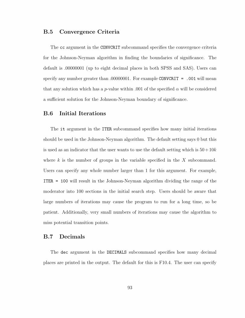
B.5 Convergence Criteria

The cc argument in the CONVCRIT subcommand specifies the convergence criteria

for the Johnson-Neyman algorithm in finding the boundaries of significance. The

default is .00000001 (up to eight decimal places in both SPSS and SAS). Users can

specify any number greater than .00000001. For example CONVCRIT = .001 will mean

that any solution which has a p-value within .001 of the specified α will be considered

a sufficient solution for the Johnson-Neyman boundary of significance.

B.6 Initial Iterations

The it argument in the ITER subcommand specifies how many initial iterations

should be used in the Johnson-Neyman algorithm. The default setting says 0 but this

is used as an indicator that the user wants to use the default setting which is 50+10k

where k is the number of groups in the variable specified in the X subcommand.

Users can specify any whole number larger than 1 for this argument. For example,

ITER = 100 will result in the Johnson-Neyman algorithm dividing the range of the

moderator into 100 sections in the initial search step. Users should be aware that

large numbers of iterations may cause the program to run for a long time, so be

patient. Additionally, very small numbers of iterations may cause the algorithm to

miss potential transition points.

B.7 Decimals

The dec argument in the DECIMALS subcommand specifies how many decimal

places are printed in the output. The default for this is F10.4. The user can specify

93

any format which is a valid printable numeric format (See SPSS Manual ). For

example DECIMALS = F10.2 will print all outputs to two decimal places.

94

Appendix C: OGRS Macro for SAS

The following is the macro code for OGRS in SAS. This code, unaltered, typed

into a syntax window and run in SAS will define OGRS such that it can be used as

described in this manuscript.

*OGRS for SPSS Version 1.1;

* Copyright 2016;

* by Amanda Kay Montoya;

* Documentation available by email to montoya.29@osu.edu;

%macro RedR (center = );

mcent = m - &center;

m2int = mcent#data[,2:numgroup];

datam2 = J(Ninit,1,1)||mcent||m2int;

IF (covtog = 1) then datam2 = datam2||cov;

yestm2 = datam2*inv((datam2‘)*datam2)*datam2‘*y;

ycorm2 = CORR(yestm2||y);

ycorm2 = ycorm2[1,2];

redr2 = ycorm2**2;

%mend;

%macro PROBE (min = , max = );

jump = (&max - &min)/iter;

dim = (transtog = 0)*(iter+1) + (transtog = 1)*(iter-1);

tempres = J(dim, 8, -999);

IF (transtog = 0) then i2 = &min;

IF (transtog = 1) then i2 = &min + jump;

DO i = 1 TO dim;

%RedR(center = i2);

tempres[i, 1:2] = i2||redr2;

i2 = i2 + jump;

END;

tempres[,3] = fullr2 - tempres[,2];

95

tempres[,4] = (dffull*tempres[,3])/(dfred*(1-fullr2));

tempres[,5] = 1 - CDF(’F’,tempres[,4],dfred,dffull);

%mend;

%macro OGRS (data =, vars =, x = , m = , y = , conf = 95,

convcrit = .00000001, decimals = 10.4, iter = 0);

proc iml;

start = time();

USE &data;

READ all var{&vars} into allvars;

allnames = {&vars};

READ all var{&x} into xdat;

xname = {&x};

READ all var{&m} into mdat;

mname = {&m};

READ all var{&y} into ydat;

yname = {&y};

convcrit = &convcrit;

conf = &conf;

alpha = 1-conf/100;

covtog = (ncol(allvars) - 3 > 0);

Ninit = nrow(allvars);

IF covtog=1 THEN DO;

covcount = 1;

cov = J(Ninit, ncol(allvars)-3, 999);

covname = J(1, ncol(allvars)-3, "AAAAAAAAAAAA");

END;

DO i = 1 TO ncol(allnames);

IF (allnames[,i] = xname) THEN DO;

x = allvars[,i];

END;

IF (allnames[,i] = mname) THEN DO;

m = allvars[,i];

END;

IF (allnames[,i] = yname) THEN DO;

y = allvars[,i];

END;

IF all(allnames[,i] ^= xname||mname||yname) THEN DO;

IF covtog = 1 THEN DO;

cov[,covcount] = allvars[,i];

covname[,covcount] = allnames[,i];

covcount = covcount + 1;

END;

END;

END;

96

designx = design(x);

numgroup = ncol(designx);

designx = designx[,1:(numgroup-1)];

xmat = J(ncol(designx)+1, ncol(designx) + 1, -999);

DO kloop = 1 TO ncol(designx);

icount = 1;

DO WHILE (xmat[kloop,1] = -999);

IF designx[icount,kloop] = 1 THEN xmat[kloop,1] = x[icount,1];

icount = icount + 1;

END;

END;

icount = 1;

DO WHILE (xmat[ncol(designx)+1,1] = -999);

IF all(designx[icount,] = 0) THEN DO;

xmat[ncol(designx)+1,] = x[icount,1]||J(1,ncol(designX),0);

END;

icount = icount +1;

END;

xmat[1:(numgroup-1),2:numgroup] = I(numgroup-1);

prodcol = designX#m;

IF covtog = 0 THEN data = J(Ninit,1,1)||designX||m||prodcol;

IF covtog = 1 THEN data = J(Ninit,1,1)||designX||m||prodcol||cov;

yest = data*inv(data‘*data)*data‘*y;

ycor = corr(y||yest);

ycor = ycor[1,2];

fullr2 = ycor**2;

IF &iter = 0 THEN iter = 50+10*numgroup;

IF &iter ^= 0 THEN iter = &iter;

dffull = Ninit - ncol(data);

dfred = numgroup - 1;

Ffull = (fullr2*dffull)/((1-fullr2)*(ncol(data)-1));

pfull = 1 - CDF(’F’,Ffull,(ncol(data)-1),dffull);

critF = FINV(conf/100, dfred, dffull);

modres = J(ncol(data), 6, -999);

modres[,1] = inv(data‘*data)*data‘*y;

ssr = sum((y-yest)##2);

msr = ssr/(Ninit - ncol(data));

semat = msr*inv(data‘*data);

modres[,2] = (vecdiag(semat))##(1/2);

modres[,3] = modres[,1]/modres[,2];

modres[,4] = 2*(1-CDF(’t’, abs(modres[,3]),dffull));

tcrit = TINV(1-alpha/2, dffull);

modres[,5] = modres[,1] - tcrit*modres[,2];

modres[,6] = modres[,1] + tcrit*modres[,2];

dataint = J(Ninit, 1,1)||designx||m;

97

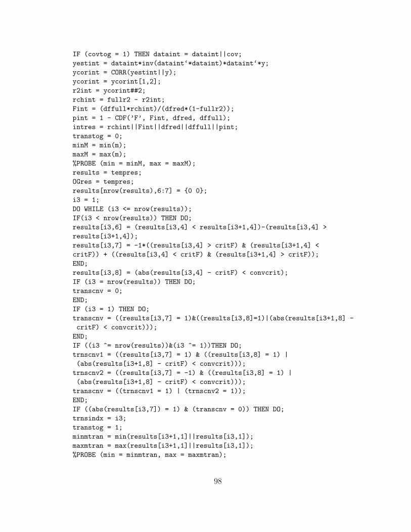
IF (covtog = 1) THEN dataint = dataint||cov;

yestint = dataint*inv(dataint‘*dataint)*dataint‘*y;

ycorint = CORR(yestint||y);

ycorint = ycorint[1,2];

r2int = ycorint##2;

rchint = fullr2 - r2int;

Fint = (dffull*rchint)/(dfred*(1-fullr2));

pint = 1 - CDF(’F’, Fint, dfred, dffull);

intres = rchint||Fint||dfred||dffull||pint;

transtog = 0;

minM = min(m);

maxM = max(m);

%PROBE (min = minM, max = maxM);

results = tempres;

OGres = tempres;

results[nrow(results),6:7] = {0 0};

i3 = 1;

DO WHILE (i3 <= nrow(results));

IF(i3 < nrow(results)) THEN DO;

results[i3,6] = (results[i3,4] < results[i3+1,4])-(results[i3,4] >

results[i3+1,4]);

results[i3,7] = -1*((results[i3,4] > critF) & (results[i3+1,4] <

critF)) + ((results[i3,4] < critF) & (results[i3+1,4] > critF));

END;

results[i3,8] = (abs(results[i3,4] - critF) < convcrit);

IF (i3 = nrow(results)) THEN DO;

transcnv = 0;

END;

IF (i3 = 1) THEN DO;

transcnv = ((results[i3,7] = 1)&((results[i3,8]=1)|(abs(results[i3+1,8] -

critF) < convcrit)));

END;

IF ((i3 ^= nrow(results))&(i3 ^= 1))THEN DO;

trnscnv1 = ((results[i3,7] = 1) & ((results[i3,8] = 1) |

(abs(results[i3+1,8] - critF) < convcrit)));

trnscnv2 = ((results[i3,7] = -1) & ((results[i3,8] = 1) |

(abs(results[i3+1,8] - critF) < convcrit)));

transcnv = ((trnscnv1 = 1) | (trnscnv2 = 1));

END;

IF ((abs(results[i3,7]) = 1) & (transcnv = 0)) THEN DO;

trnsindx = i3;

transtog = 1;

minmtran = min(results[i3+1,1]||results[i3,1]);

maxmtran = max(results[i3+1,1]||results[i3,1]);

%PROBE (min = minmtran, max = maxmtran);

98

results = results//tempres;

CALL sort(results,1);

END;

IF ((abs(results[i3,7]) = 0) | (transcnv = 1)) THEN i3 = i3+1;

END;

numJN = (results[nrow(results),8]=1)+((results[1,8] = 1) &

(results[1,7] ^= 1)) + sum(abs(results[,7]));

IF (numJN > 0) THEN DO;

JNSoln = J(numJN, 1, -999);

JNIndx = J(numJN, 1, -999);

slncnt = 1;

IF (results[nrow(results),8] = 1) THEN DO;

JNSoln[1,1] = results[nrow(results),1];

JNIndx[1,1] = nrow(results);

slncnt = slncnt + 1;

END;

DO i1 = 1 to nrow(results);

IF (abs(results[i1,7]) = 1) then do;

abvblw = (results[i1,1]||abs(results[i1,4] - critF))//(results[i1+1,1]||

abs(results[i1+1,4] - critF));

unsort = abvblw;

CALL sort(abvblw,2);

JNSoln[slncnt,1] = abvblw[1,1];

indxtog = all(abvblw = unsort);

IF (indxtog = 1) THEN JNIndx[slncnt,1] = i1;

IF (indxtog = 0) THEN JNIndx[slncnt,1] = i1+1;

slncnt = slncnt + 1;

END;

END;

END;

PRINT "************************ OGRS Procedure for SAS Version 1.1

*************************";

PRINT "Written by Amanda K. Montoya";

PRINT "Documentation available by request";

PRINT "*******************************************************

*************************************";

varrlabs = {"X = " "M = " "Y = "};

PRINT (xname//mname//yname) [label = "Variables:" rowname = varrlabs];

IF (covtog = 1) THEN DO;

PRINT covname [label = "Statistical Controls:"];

END;

dummylab = {"D1" "D2" "D3" "D4" "D5" "D6" "D7" "D8" "D9"};

xmatlab = xname||dummylab[1,1:(numgroup-1)];

PRINT xmat [label = "Dummy Variable Coding Scheme:" colname = xmatlab];

PRINT Ninit [label = "Sample Size:"];

99

PRINT "********************************************************************

************************";

PRINT yname [label = "Outcome:"];

modsum = sqrt(fullr2)||fullr2||Ffull||(ncol(data)-1)||dffull||pfull;

PRINT modsum [label = "Model Summary" colname = {"R" "R-Sq" "F" "df1" "df2"

"p"} format = &decimals];

intlab = {"Int1" "Int2" "Int3" "Int4" "Int5" "Int6" "Int7" "Int8" "Int9"};

modlabs = "Constant"||dummylab[1,1:(numgroup-1)]||mname||intlab[1,1:

(numgroup-1)];

IF (covtog = 1) THEN modlabs = modlabs||covname;

PRINT modres [label = "Model" rowname = modlabs colname = {"coeff" "SE" "t"

"p" "LLCI" "ULCI"} format = &decimals];

intmat = J((numgroup-1),5,"AAAAAAAAAAAA");

intmat[,1] = (intlab[1,1:(numgroup-1)])‘;

intmat[,2] = J((numgroup-1),1, "=");

intmat[,3] = (dummylab[1,1:(numgroup-1)])‘;

intmat[,4] = J((numgroup-1),1,"X");

intmat[,5] = J((numgroup-1), 1, mname);

PRINT intmat [label = "Interactions:"];

PRINT intres [label = "R-Square increase due to interaction(s):"

colname = {"R2-chng" "F" "df1" "df2" "p"} format = &decimals];

PRINT "************************* JOHNSON-NEYMAN TECHNIQUE

*************************";

IF (iter > 10) THEN DO;

last = nrow(OGres);

rjump = ceil(last/20);

rowsel = 1;

rcount = 1+rjump;

DO WHILE (rcount <= last);

rowsel = rowsel||rcount;

rcount = rcount +rjump;

END;

IF (rcount-rjump ^= last) THEN rowsel = rowsel||last;

END;

JNtabnam = mname||"R2-chng"||"F"||"p";

IF (numJN > 0) THEN DO;

PRINT JNSoln [label = "Moderator value(s) defining Johnson-Neyman boundaries

of significance;" format = &decimals];

IF (iter > 10) THEN DO;

JNouttab = OGres[rowsel,]//results[JNIndx,];

END;

IF (iter <= 10) THEN DO;

JNouttab = OGres//results[JNIndx,];

END;

CALL sort(JNouttab,1);

100

JNouttab = JNouttab[,{1 3 4 5}];

END;

IF (numJN = 0) THEN DO;

PRINT "No Johnson-Neyman bounds found within the range of observed data";

IF (iter > 10) THEN JNouttab = OGres[rowsel,{1 3 4 5}];

IF (iter <= 10) THEN JNouttab = OGres[,{1 3 4 5}];

END;

PRINT JNouttab [label = "Conditional effect of X on Y at values of the

moderator (M)" colname = JNtabnam format = &decimals];

PRINT "**********************************************************

*******************";

quit;

%mend;

101

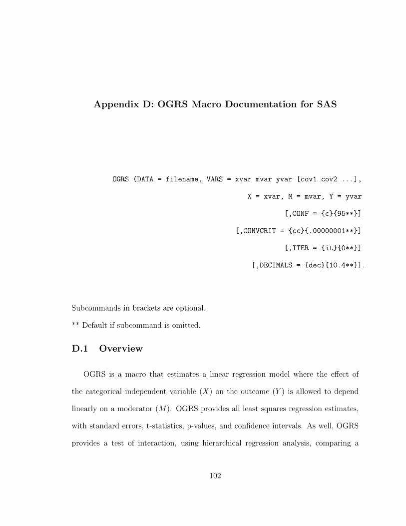
Appendix D: OGRS Macro Documentation for SAS

OGRS (DATA = filename, VARS = xvar mvar yvar [cov1 cov2 ...],

X = xvar, M = mvar, Y = yvar

[,CONF = {c}{95**}]

[,CONVCRIT = {cc}{.00000001**}]

[,ITER = {it}{0**}]

[,DECIMALS = {dec}{10.4**}].

Subcommands in brackets are optional.

** Default if subcommand is omitted.

D.1 Overview

OGRS is a macro that estimates a linear regression model where the effect of

the categorical independent variable (X) on the outcome (Y ) is allowed to depend

linearly on a moderator (M). OGRS provides all least squares regression estimates,

with standard errors, t-statistics, p-values, and confidence intervals. As well, OGRS

provides a test of interaction, using hierarchical regression analysis, comparing a

102

model where the effect of X is allowed to vary linearly with M and a model where

the effect of X is fixed across M .

OGRS also provides a unique method for probing the effect of X on Y using

an approximation of the Johnson-Neyman procedure. OGRS searches the observed

range of the moderator for points at which the effect of X on Y transitions from

significant to non-significant or vice versa, as specified by some level of confidence

(CONF). OGRS prints the transition points if any exist within the observed range of

the moderator, as well as a table of points along the moderator, statistics related to

the estimated effect of X at that point, and inferential statistics for the effect of X.

D.2 Preparation for Use

The OGRS.sas file should be opened as a program file in SAS. Once opened,

execute the entire file exactly as is. Do not modify the code. Once the program

is executed, the OGRS.sas file window can be closed. Once executed, access to the

OGRS command is available until quitting SAS. The OGRS.sas file must be loaded

and re-executed each time SAS is opened.

D.3 Model Specification

Because OGRS will only accept one variable in the X subcommand, your inde-

pendent variable should be coded into one variable, with unique codes for each group.

Categorical independent variables can represent groups (e.g. race, political party),

experimental conditions, or any other categorical variable of interest. Both the mod-

erator M and the outcome variable Y are treated as continuous variables. Covariates

103

specified in the model can be continuous or dichotomous, but they cannot be cate-

gorical with more than two groups. To use categorical covariates, using your desired

coding scheme (e.g. dummy coding) to create k − 1 new variables to represent your

categorical covariate, and include all of these variables as covariates in the model.

Covariates can be included in the vars subcommand, and they will be included in

the regression model.

Various options in OGRS allow you to tailor the output to your question of in-

terest. You can specify a confidence level, the convergence criteria for the Johnson-

Neyman approximation, number of initial iterations in the Johnson-Neyman approx-

imation, and the number of decimal places printed in the output. For example:

OGRS (data = datname, vars = Xvar Mvar Yvar Cov1, conf = 90,

convcrit = .0001, iter = 1000, decimals = 10.6.)

will estimate the effect of a categorical variable Xvar on Yvar moderated by Mvar.

All confidence intervals will be 90% confidence intervals, and the Johnson-Neyman

procedure will solve for points of transition along Mvar where the effect of Xvar on

Yvar is exactly significant at α = 0.10. The convergence criteria will be .0001 rather

than the typical .00000001, and the Johnson-Neyman approximation will begin with

1000 iterations. All output will be printed to six decimals places.

D.4 Confidence Level

The c argument in the CONF subcommand specifies the confidence level for all

confidence intervals and the criterion value for which the Johnson-Neyman procedure

will compute the boundaries of significance. The default is 95%. Users can specify

any confidence level greater than 50 and less than 100. For example CONF = 90 will

result in 90% confidence intervals and for the Johnson-Neyman procedure to find the

104

points along the moderator at which the effect of the independent variable on the

outcome variable is exactly significant at α = .10.

D.5 Convergence Criteria

The cc argument in the CONVCRIT subcommand specifies the convergence criteria

for the Johnson-Neyman algorithm in finding the boundaries of significance. The

default is .00000001 (up to eight decimal places in both SPSS and SAS). Users can

specify any number greater than .00000001. For example CONVCRIT = .001 will mean

that any solution which has a an F -statistic within .001 of the criterion F -statistic will

be considered a sufficient solution for the Johnson-Neyman boundary of significance.

D.6 Initial Iterations

The it argument in the ITER subcommand specifies how many initial iterations

should be used in the Johnson-Neyman algorithm. The default setting says 0 but this

is used as an indicator that the user wants to use the default setting which is 50+10k

where k is the number of groups in the variable specified in the X subcommand.

Users can specify any whole number larger than 1 for this argument. For example,

ITER = 100 will result in the Johnson-Neyman algorithm dividing the range of the

moderator into 100 sections in the initial search step. Users should be aware that

large numbers of iterations may cause the program to run for a long time, so be

patient. Additionally, very small numbers of iterations may cause the algorithm to

miss potential transition points.

105

D.7 Decimals

The dec argument in the DECIMALS subcommand specifies how many decimal

places are printed in the output. The default for this is F10.4. The user can specify

any format which is a valid printable numeric format (See SAS Manual ). For example

DECIMALS = 10.2 will print all outputs to two decimal places.

106