Bernoulli to Laplace Boole, Venn, Neyman, Statistical...
51
Learning and Teaching Statistical Inference B. Blais History Bernoulli to Laplace Boole, Venn, Neyman, Pearson, Fisher, etc. . . Cox and Jaynes Two Schools of Thought on Probability Estimating the Amplitude of a Signal Two Approaches Comparison Comparisons Hypothesis Testing Unknown mean, Known Variance Unknown mean, Unknown Variance Unknown proportion Other Examples Behrens-Fisher Flipping a Tack Conclusions Learning and Teaching Statistical Inference An Open Discussion B. Blais Department of Science and Technology Bryant University Faculty Development Seminar - Fall 2005
Transcript of Bernoulli to Laplace Boole, Venn, Neyman, Statistical...

Learning andTeachingStatisticalInference
B. Blais
HistoryBernoulli to Laplace
Boole, Venn, Neyman,Pearson, Fisher, etc. . .
Cox and Jaynes
Two Schools of Thought onProbability
Estimating theAmplitude of aSignalTwo Approaches
Comparison
ComparisonsHypothesis Testing
Unknown mean, KnownVariance
Unknown mean, UnknownVariance
Unknown proportion
Other ExamplesBehrens-Fisher
Flipping a Tack
Conclusions
Learning and TeachingStatistical Inference
An Open Discussion
B. Blais
Department of Science and TechnologyBryant University
Faculty Development Seminar - Fall 2005

Learning andTeachingStatisticalInference
B. Blais
HistoryBernoulli to Laplace
Boole, Venn, Neyman,Pearson, Fisher, etc. . .
Cox and Jaynes
Two Schools of Thought onProbability
Estimating theAmplitude of aSignalTwo Approaches
Comparison
ComparisonsHypothesis Testing
Unknown mean, KnownVariance
Unknown mean, UnknownVariance
Unknown proportion
Other ExamplesBehrens-Fisher
Flipping a Tack
Conclusions
Abstract
This Faculty Development Seminar focuses on thelearning and teaching of statistical inference, and isdirected towards those who use statistics andstatistical inference in either their teaching orresearch. During my summer vacation, I took theopportunity to learn and re-learn basic statistics. Inthis seminar, I would like to share what I havediscovered in my studies, including some interestinghistory and pedagogy. I would like to then introducesome possible alternative approaches to teachingstatistical inference, and open up the discussion toevaluate these suggestions and to get suggestionsfrom the faculty for whom statistical inference plays alarge role in their classroom. I would like to explorestudent misperceptions and challenges, along withinteresting pedagogical examples which highlight theimportant aspects of statistical inference.

Learning andTeachingStatisticalInference
B. Blais
HistoryBernoulli to Laplace
Boole, Venn, Neyman,Pearson, Fisher, etc. . .
Cox and Jaynes
Two Schools of Thought onProbability
Estimating theAmplitude of aSignalTwo Approaches
Comparison
ComparisonsHypothesis Testing
Unknown mean, KnownVariance
Unknown mean, UnknownVariance
Unknown proportion
Other ExamplesBehrens-Fisher
Flipping a Tack
Conclusions
Some Data
What does the “∗” mean?
How can one objectively define “significance”?
What are the assumptions?

Learning andTeachingStatisticalInference
B. Blais
HistoryBernoulli to Laplace
Boole, Venn, Neyman,Pearson, Fisher, etc. . .
Cox and Jaynes
Two Schools of Thought onProbability
Estimating theAmplitude of aSignalTwo Approaches
Comparison
ComparisonsHypothesis Testing
Unknown mean, KnownVariance
Unknown mean, UnknownVariance
Unknown proportion
Other ExamplesBehrens-Fisher
Flipping a Tack
Conclusions
Food For Thought
What does the word probability mean?
Why do we say that a coin has phead= 0.5?
What do we mean by identical repetitions?
Learning andTeachingStatisticalInference
B. Blais
HistoryBernoulli to Laplace
Boole, Venn, Neyman,Pearson, Fisher, etc. . .
Cox and Jaynes
Two Schools of Thought onProbability
Estimating theAmplitude of aSignalTwo Approaches
Comparison
ComparisonsHypothesis Testing
Unknown mean, KnownVariance
Unknown mean, UnknownVariance
Unknown proportion
Other ExamplesBehrens-Fisher
Flipping a Tack
Conclusions
Outline1 History
Bernoulli to LaplaceBoole, Venn, Neyman, Pearson, Fisher, etc. . .Cox and JaynesTwo Schools of Thought on Probability
2 Estimating the Amplitude of a SignalTwo ApproachesComparison
3 ComparisonsHypothesis TestingUnknown mean, Known VarianceUnknown mean, Unknown VarianceUnknown proportion
4 Other ExamplesBehrens-FisherFlipping a Tack
5 Conclusions
Learning andTeachingStatisticalInference
B. Blais
HistoryBernoulli to Laplace
Boole, Venn, Neyman,Pearson, Fisher, etc. . .
Cox and Jaynes
Two Schools of Thought onProbability
Estimating theAmplitude of aSignalTwo Approaches
Comparison
ComparisonsHypothesis Testing
Unknown mean, KnownVariance
Unknown mean, UnknownVariance
Unknown proportion
Other ExamplesBehrens-Fisher
Flipping a Tack
Conclusions
History: Bernoulli
James Bernoulli (1713) in “Ars Conjectandi”: definedprobability as a “degree of certainty”.
His theorem states that, if the probability of an eventis p then the limiting frequency of that eventconverges to p.

Learning andTeachingStatisticalInference
B. Blais
HistoryBernoulli to Laplace
Boole, Venn, Neyman,Pearson, Fisher, etc. . .
Cox and Jaynes
Two Schools of Thought onProbability
Estimating theAmplitude of aSignalTwo Approaches
Comparison
ComparisonsHypothesis Testing
Unknown mean, KnownVariance
Unknown mean, UnknownVariance
Unknown proportion
Other ExamplesBehrens-Fisher
Flipping a Tack
Conclusions
History: Bernoulli
Example: Coin with phead= 0.4, N flips
p(m|N) =
(Nm
)0.4m(1− 0.4)N−m
as N →∞, observed frequency f ≡ mN → 0.4
0
5
10
15
20
25
30
0 0.1 0.2 0.3 0.4 0.5 0.6 0.7 0.8 0.9 1
prob
abili
ty d
ensi
ty
Frequency (f := m/N)
N=20N=100
N=1000
Learning andTeachingStatisticalInference
B. Blais
HistoryBernoulli to Laplace
Boole, Venn, Neyman,Pearson, Fisher, etc. . .
Cox and Jaynes
Two Schools of Thought onProbability
Estimating theAmplitude of aSignalTwo Approaches
Comparison
ComparisonsHypothesis Testing
Unknown mean, KnownVariance
Unknown mean, UnknownVariance
Unknown proportion
Other ExamplesBehrens-Fisher
Flipping a Tack
Conclusions
History: Bernoulli
Assignment of probabilities: Principle of InsufficientReason
If the evidence does not provide any reason to chooseproposition A1 or A2, then one assigns equal probability toboth.
Equivalent states of knowledge (say, swapping labels 1and 2) should yield identical probability assignments.
Generalizes to N propositions
p(A) =mN
=(number of cases favorable to A)
(total number of equally possible cases)
Learning andTeachingStatisticalInference
B. Blais
HistoryBernoulli to Laplace
Boole, Venn, Neyman,Pearson, Fisher, etc. . .
Cox and Jaynes
Two Schools of Thought onProbability
Estimating theAmplitude of aSignalTwo Approaches
Comparison
ComparisonsHypothesis Testing
Unknown mean, KnownVariance
Unknown mean, UnknownVariance
Unknown proportion
Other ExamplesBehrens-Fisher
Flipping a Tack
Conclusions
History: Bernoulli, Bayes, Laplace
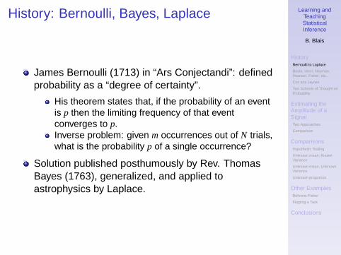
James Bernoulli (1713) in “Ars Conjectandi”: definedprobability as a “degree of certainty”.
His theorem states that, if the probability of an eventis p then the limiting frequency of that eventconverges to p.Inverse problem: given m occurrences out of N trials,what is the probability p of a single occurrence?
Solution published posthumously by Rev. ThomasBayes (1763), generalized, and applied toastrophysics by Laplace.
Learning andTeachingStatisticalInference
B. Blais
HistoryBernoulli to Laplace
Boole, Venn, Neyman,Pearson, Fisher, etc. . .
Cox and Jaynes
Two Schools of Thought onProbability
Estimating theAmplitude of aSignalTwo Approaches
Comparison
ComparisonsHypothesis Testing
Unknown mean, KnownVariance
Unknown mean, UnknownVariance
Unknown proportion
Other ExamplesBehrens-Fisher
Flipping a Tack
Conclusions
History: Bayes, Laplace
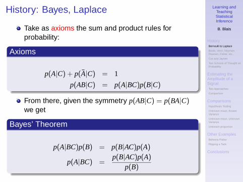
Take as axioms the sum and product rules forprobability:
Axioms
p(A|C) + p(A|C) = 1
p(AB|C) = p(A|BC)p(B|C)
From there, given the symmetry p(AB|C) = p(BA|C)we get
Bayes’ Theorem
p(A|BC)p(B) = p(B|AC)p(A)
p(A|BC) =p(B|AC)p(A)
p(B)
Learning andTeachingStatisticalInference
B. Blais
HistoryBernoulli to Laplace
Boole, Venn, Neyman,Pearson, Fisher, etc. . .
Cox and Jaynes
Two Schools of Thought onProbability
Estimating theAmplitude of aSignalTwo Approaches
Comparison
ComparisonsHypothesis Testing
Unknown mean, KnownVariance
Unknown mean, UnknownVariance
Unknown proportion
Other ExamplesBehrens-Fisher
Flipping a Tack
Conclusions
History: Laplace
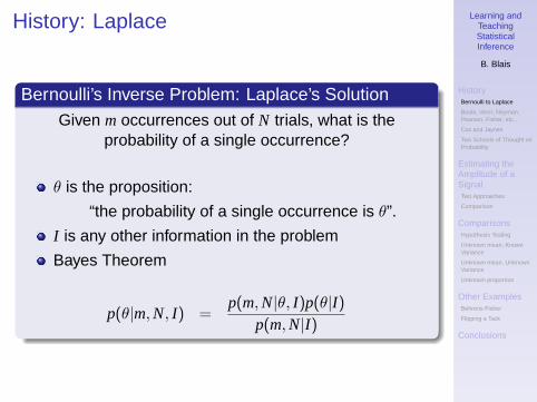
Bernoulli’s Inverse Problem: Laplace’s SolutionGiven m occurrences out of N trials, what is the
probability of a single occurrence?
θ is the proposition:
“the probability of a single occurrence is θ”.
I is any other information in the problem
Bayes Theorem
p(θ|m, N, I) =p(m, N|θ, I)p(θ|I)
p(m, N|I)
Learning andTeachingStatisticalInference
B. Blais
HistoryBernoulli to Laplace
Boole, Venn, Neyman,Pearson, Fisher, etc. . .
Cox and Jaynes
Two Schools of Thought onProbability
Estimating theAmplitude of aSignalTwo Approaches
Comparison
ComparisonsHypothesis Testing
Unknown mean, KnownVariance
Unknown mean, UnknownVariance
Unknown proportion
Other ExamplesBehrens-Fisher
Flipping a Tack
Conclusions
History: Laplace
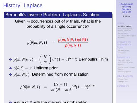
Bernoulli’s Inverse Problem: Laplace’s SolutionGiven m occurrences out of N trials, what is the
probability of a single occurrence?
p(θ|m, N, I) =p(m, N|θ, I)p(θ|I)
p(m, N|I)
p(m, N|θ, I) =
(Nm
)θm(1− θ)N−m: Bernoulli’s Th’m
p(θ|I) = 1: Uniform prior
p(m, N|I): Determined from normalization
p(θ|m, N, I) =(N + 1)!
m!(N−m)!θm(1− θ)N−m
Value of θ with the maximum probability:
θ =mN

Learning andTeachingStatisticalInference
B. Blais
HistoryBernoulli to Laplace
Boole, Venn, Neyman,Pearson, Fisher, etc. . .
Cox and Jaynes
Two Schools of Thought onProbability
Estimating theAmplitude of aSignalTwo Approaches
Comparison
ComparisonsHypothesis Testing
Unknown mean, KnownVariance
Unknown mean, UnknownVariance
Unknown proportion
Other ExamplesBehrens-Fisher
Flipping a Tack
Conclusions
History: Boole, Venn, Neyman, Pearson,Fisher, etc. . .
Criticisms of Laplace1 The axioms are not clearly unique for a definition of
probability as vague as “degrees of plausibility”.Algebra of relative frequencies satisfies the axioms
2 It was unclear how to assign the prior probabilities ofpropositions in the first place: how to generalizeBernoulli’s Principle of Insufficient Reason forcontinuous cases?Problem disappears: meaningless to speak of aprobability of propositions because there is nolimiting frequency (always true, or always false).
Solution:
define probability as the long-run relative frequency ofoccurrence
Learning andTeachingStatisticalInference
B. Blais
HistoryBernoulli to Laplace
Boole, Venn, Neyman,Pearson, Fisher, etc. . .
Cox and Jaynes
Two Schools of Thought onProbability
Estimating theAmplitude of aSignalTwo Approaches
Comparison
ComparisonsHypothesis Testing
Unknown mean, KnownVariance
Unknown mean, UnknownVariance
Unknown proportion
Other ExamplesBehrens-Fisher
Flipping a Tack
Conclusions
History: Birth of Statistics
Hypotheses are either true or false for the entirepopulation, and thus do not have a long-run relativefrequency.
Create a statistic: any function of the observedrandom variables in a sample, without any unknownquantities, e.g.
Sample mean: x =1N
∑i
xi
Sample variance: S2 =1
N− 1
∑i
(xi − x)2
Criteria for choosing a statistic: unbiasedness,efficiency, consistency, coherence, sufficiency, thelikelihood principle, etc. . .
Learning andTeachingStatisticalInference
B. Blais
HistoryBernoulli to Laplace
Boole, Venn, Neyman,Pearson, Fisher, etc. . .
Cox and Jaynes
Two Schools of Thought onProbability
Estimating theAmplitude of aSignalTwo Approaches
Comparison
ComparisonsHypothesis Testing
Unknown mean, KnownVariance
Unknown mean, UnknownVariance
Unknown proportion
Other ExamplesBehrens-Fisher
Flipping a Tack
Conclusions
History: R. T. Cox and E. T. Jaynes
Axioms for Probability Theory1 Degrees of plausibility are represented by real
numbers2 Qualitative correspondence with common sense.
Consistent with deductive logic in the limit of true andfalse propositions.
3 Consistency1 If a conclusion can be reasoned out in more than one
way, every possible way must lead to the same result2 The theory must use all of the information provided3 Equivalent states of knowledge must be represented
by equivalent plausibility assignments
Bayesian formulation uniquely satisfies these criteria

Learning andTeachingStatisticalInference
B. Blais
HistoryBernoulli to Laplace
Boole, Venn, Neyman,Pearson, Fisher, etc. . .
Cox and Jaynes
Two Schools of Thought onProbability
Estimating theAmplitude of aSignalTwo Approaches
Comparison
ComparisonsHypothesis Testing
Unknown mean, KnownVariance
Unknown mean, UnknownVariance
Unknown proportion
Other ExamplesBehrens-Fisher
Flipping a Tack
Conclusions
History: E. T. Jaynes
Generalization of the Principle of IndifferenceMaximum Entropy
Measure of the uncertainty, H, of a distribution,(p1, p2, . . ., pn), called the entropyPrior probabilities are assigned as those with themaximum entropy, given the initial information of theproblem
Transformation groupsEqual states of knowledge yield equal probabilityassignments
Learning andTeachingStatisticalInference
B. Blais
HistoryBernoulli to Laplace
Boole, Venn, Neyman,Pearson, Fisher, etc. . .
Cox and Jaynes
Two Schools of Thought onProbability
Estimating theAmplitude of aSignalTwo Approaches
Comparison
ComparisonsHypothesis Testing
Unknown mean, KnownVariance
Unknown mean, UnknownVariance
Unknown proportion
Other ExamplesBehrens-Fisher
Flipping a Tack
Conclusions
Two Schools of Thought on Probability
Frequentist Statistical Inferencep(A) =long-run relative frequency with which A occurs inidentical repeats of an experiment.“A” restricted to propositions about random variables.
Bayesian Inferencep(A|B) =a real number measure of the plausibility of aproposition/hypothesis A, given (conditional on) the truthof the information represented by proposition B.“A” can be any logical proposition, not restricted topropositions about random variables.
Learning andTeachingStatisticalInference
B. Blais
HistoryBernoulli to Laplace
Boole, Venn, Neyman,Pearson, Fisher, etc. . .
Cox and Jaynes
Two Schools of Thought onProbability
Estimating theAmplitude of aSignalTwo Approaches
Comparison
ComparisonsHypothesis Testing
Unknown mean, KnownVariance
Unknown mean, UnknownVariance
Unknown proportion
Other ExamplesBehrens-Fisher
Flipping a Tack
Conclusions
Objective versus Subjective
Bayesian inference is often labeled as subjective,because the probability is a measure of a state ofknowledge, and not directly observable like a relativefrequency
Loredo 1990: “In this sense, Bayesian ProbabilityTheory is ‘subjective,’ it describes states ofknowledge, not states of nature. But it is ‘objective’ inthat we insist that equivalent states of knowledge berepresented by equal probabilities, and that problemsbe well-posed: enough information must be providedto allow unique, unambiguous probabilityassignments.”
Learning andTeachingStatisticalInference
B. Blais
HistoryBernoulli to Laplace
Boole, Venn, Neyman,Pearson, Fisher, etc. . .
Cox and Jaynes
Two Schools of Thought onProbability
Estimating theAmplitude of aSignalTwo Approaches
Comparison
ComparisonsHypothesis Testing
Unknown mean, KnownVariance
Unknown mean, UnknownVariance
Unknown proportion
Other ExamplesBehrens-Fisher
Flipping a Tack
Conclusions
Definition of the Problem
Magnitude of a signal, µ
Given N measurements, xi , contaminated with noisewith known standard deviation, σ
Learning andTeachingStatisticalInference
B. Blais
HistoryBernoulli to Laplace
Boole, Venn, Neyman,Pearson, Fisher, etc. . .
Cox and Jaynes
Two Schools of Thought onProbability
Estimating theAmplitude of aSignalTwo Approaches
Comparison
ComparisonsHypothesis Testing
Unknown mean, KnownVariance
Unknown mean, UnknownVariance
Unknown proportion
Other ExamplesBehrens-Fisher
Flipping a Tack
Conclusions
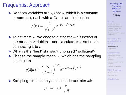
Frequentist Approach
Random variables are xi (not µ, which is a constantparameter), each with a Gaussian distribution
p(xi) =1√
2πσ2e−(xi−µ)2/2σ2
To estimate µ, we choose a statistic – a function ofthe random variables – and calculate its distributionconnecting it to µWhat is the “best” statistic? unbiased? sufficient?Choose the sample mean, x, which has the samplingdistribution
p(x|µ) =
(N
2πσ2
)1/2
e−N(x−µ)2/2σ2
Sampling distribution yields confidence intervals
µ = x± σ√N
Learning andTeachingStatisticalInference
B. Blais
HistoryBernoulli to Laplace
Boole, Venn, Neyman,Pearson, Fisher, etc. . .
Cox and Jaynes
Two Schools of Thought onProbability
Estimating theAmplitude of aSignalTwo Approaches
Comparison
ComparisonsHypothesis Testing
Unknown mean, KnownVariance
Unknown mean, UnknownVariance
Unknown proportion
Other ExamplesBehrens-Fisher
Flipping a Tack
Conclusions
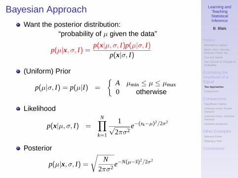
Bayesian Approach
Want the posterior distribution:“probability of µ given the data”
p(µ|x, σ, I) =p(x|µ, σ, I)p(µ|σ, I)
p(x|σ, I)
(Uniform) Prior
p(µ|σ, I) = p(µ|I) =
{A µmin ≤ µ ≤ µmax
0 otherwise
Likelihood
p(x|µ, σ, I) =N∏
k=1
1√2πσ2
e−(xk−µ)2/2σ2
Posterior
p(µ|x, σ, I) =
√N
2πσ2e−N(µ−x)2/2σ2
Learning andTeachingStatisticalInference
B. Blais
HistoryBernoulli to Laplace
Boole, Venn, Neyman,Pearson, Fisher, etc. . .
Cox and Jaynes
Two Schools of Thought onProbability
Estimating theAmplitude of aSignalTwo Approaches
Comparison
ComparisonsHypothesis Testing
Unknown mean, KnownVariance
Unknown mean, UnknownVariance
Unknown proportion
Other ExamplesBehrens-Fisher
Flipping a Tack
Conclusions
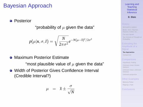
Bayesian Approach
Posterior
“probability of µ given the data”
p(µ|x, σ, I) =
√N
2πσ2e−N(µ−x)2/2σ2
Maximum Posterior Estimate
“most plausible value of µ given the data”
Width of Posterior Gives Confidence Interval(Credible Interval?)
µ = x± σ√N
Learning andTeachingStatisticalInference
B. Blais
HistoryBernoulli to Laplace
Boole, Venn, Neyman,Pearson, Fisher, etc. . .
Cox and Jaynes
Two Schools of Thought onProbability
Estimating theAmplitude of aSignalTwo Approaches
Comparison
ComparisonsHypothesis Testing
Unknown mean, KnownVariance
Unknown mean, UnknownVariance
Unknown proportion
Other ExamplesBehrens-Fisher
Flipping a Tack
Conclusions
Comparison
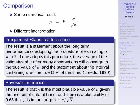
Same numerical result
µ = x± σ√N
Different interpretation
Frequentist Statistical InferenceThe result is a statement about the long termperformance of adopting the procedure of estimating µwith x. If one adopts this procedure, the average of theestimates of µ after many observations will converge tothe true value of µ, and the statement about the intervalcontaining µ will be true 68% of the time. (Loredo, 1990)
Bayesian InferenceThe result is that x is the most plausible value of µ giventhe one set of data at hand, and there is a plausibility of0.68 that µ is in the range x± σ/
√N.
Learning andTeachingStatisticalInference
B. Blais
HistoryBernoulli to Laplace
Boole, Venn, Neyman,Pearson, Fisher, etc. . .
Cox and Jaynes
Two Schools of Thought onProbability
Estimating theAmplitude of aSignalTwo Approaches
Comparison
ComparisonsHypothesis Testing
Unknown mean, KnownVariance
Unknown mean, UnknownVariance
Unknown proportion
Other ExamplesBehrens-Fisher
Flipping a Tack
Conclusions
Frequentist: Hypothesis Testing and p Values
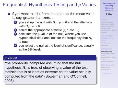
If you want to infer from the data that the mean valueis, say, greater than zero. . .
1 you set up the null with Ho : µ = 0 and the alternatewith Ha : µ > 0
2 select the appropriate statistic (z, t, etc. . . )3 calculate the p-value of the null, where you use
hypothetical data and look for the frequency that Ho
is true.4 you reject the null at the level of significance, usually
at the 5% level.
p value“the probability, computed assuming that the nullhypothesis Ho is true, of observing a value of the teststatistic that is at least as extreme as the value actuallycomputed from the data” (Bowerman and O’Connell,2003).
Learning andTeachingStatisticalInference
B. Blais
HistoryBernoulli to Laplace
Boole, Venn, Neyman,Pearson, Fisher, etc. . .
Cox and Jaynes
Two Schools of Thought onProbability
Estimating theAmplitude of aSignalTwo Approaches
Comparison
ComparisonsHypothesis Testing
Unknown mean, KnownVariance
Unknown mean, UnknownVariance
Unknown proportion
Other ExamplesBehrens-Fisher
Flipping a Tack
Conclusions
Frequentist: Hypothesis Testing and p Values
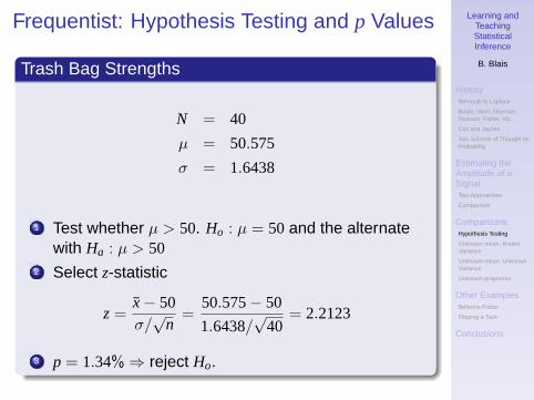
Trash Bag Strengths
N = 40
µ = 50.575
σ = 1.6438
1 Test whether µ > 50. Ho : µ = 50 and the alternatewith Ha : µ > 50
2 Select z-statistic
z =x− 50σ/√
n=
50.575− 50
1.6438/√
40= 2.2123
3 p = 1.34% ⇒ reject Ho.
Learning andTeachingStatisticalInference
B. Blais
HistoryBernoulli to Laplace
Boole, Venn, Neyman,Pearson, Fisher, etc. . .
Cox and Jaynes
Two Schools of Thought onProbability
Estimating theAmplitude of aSignalTwo Approaches
Comparison
ComparisonsHypothesis Testing
Unknown mean, KnownVariance
Unknown mean, UnknownVariance
Unknown proportion
Other ExamplesBehrens-Fisher
Flipping a Tack
Conclusions
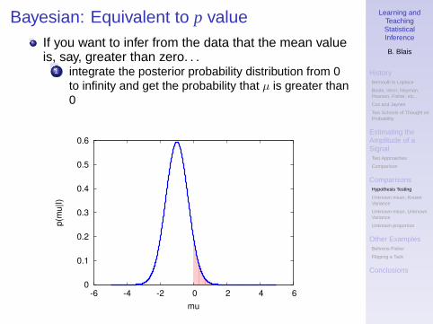
Bayesian: Equivalent to p valueIf you want to infer from the data that the mean valueis, say, greater than zero. . .
1 integrate the posterior probability distribution from 0to infinity and get the probability that µ is greater than0
0
0.1
0.2
0.3
0.4
0.5
0.6
-6 -4 -2 0 2 4 6
p(m
u|I)
mu
Learning andTeachingStatisticalInference
B. Blais
HistoryBernoulli to Laplace
Boole, Venn, Neyman,Pearson, Fisher, etc. . .
Cox and Jaynes
Two Schools of Thought onProbability
Estimating theAmplitude of aSignalTwo Approaches
Comparison
ComparisonsHypothesis Testing
Unknown mean, KnownVariance
Unknown mean, UnknownVariance
Unknown proportion
Other ExamplesBehrens-Fisher
Flipping a Tack
Conclusions
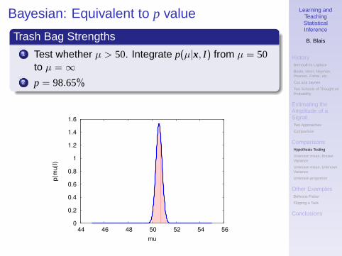
Bayesian: Equivalent to p value
Trash Bag Strengths1 Test whether µ > 50. Integrate p(µ|x, I) from µ = 50
to µ = ∞2 p = 98.65%
0
0.2
0.4
0.6
0.8
1
1.2
1.4
1.6
44 46 48 50 52 54 56
p(m
u|I)
mu

Learning andTeachingStatisticalInference
B. Blais
HistoryBernoulli to Laplace
Boole, Venn, Neyman,Pearson, Fisher, etc. . .
Cox and Jaynes
Two Schools of Thought onProbability
Estimating theAmplitude of aSignalTwo Approaches
Comparison
ComparisonsHypothesis Testing
Unknown mean, KnownVariance
Unknown mean, UnknownVariance
Unknown proportion
Other ExamplesBehrens-Fisher
Flipping a Tack
Conclusions
Bayesian Equivalents
Unknown mean, Known VariancePosterior: z-dist
p(µ|x, σ, I) =
√N
2πσ2e−N(x−µ)2/2σ2
Best Estimate
µ = x± σ√N
Learning andTeachingStatisticalInference
B. Blais
HistoryBernoulli to Laplace
Boole, Venn, Neyman,Pearson, Fisher, etc. . .
Cox and Jaynes
Two Schools of Thought onProbability
Estimating theAmplitude of aSignalTwo Approaches
Comparison
ComparisonsHypothesis Testing
Unknown mean, KnownVariance
Unknown mean, UnknownVariance
Unknown proportion
Other ExamplesBehrens-Fisher
Flipping a Tack
Conclusions
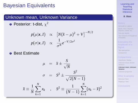
Bayesian Equivalents
Unknown mean, Unknown Variance
Posterior: t-dist, χ2
p(µ|x, I) ∝[N(x− µ)2 + V
]−N/2
p(σ|x, I) ∝ 1σN e−V/2σ2
Best Estimate
µ = x± S√N
σ = S2± S2√2(N− 1)
x≡ 1N
N∑k=1
xk , S2 ≡ 1(N− 1)
N∑k=1
(xk − x)2

Learning andTeachingStatisticalInference
B. Blais
HistoryBernoulli to Laplace
Boole, Venn, Neyman,Pearson, Fisher, etc. . .
Cox and Jaynes
Two Schools of Thought onProbability
Estimating theAmplitude of aSignalTwo Approaches
Comparison
ComparisonsHypothesis Testing
Unknown mean, KnownVariance
Unknown mean, UnknownVariance
Unknown proportion
Other ExamplesBehrens-Fisher
Flipping a Tack
Conclusions
Bayesian Equivalents
Unknown proportionPosterior: β-dist
p(θ|D, I) =(N + 1)!
m!(N−m)!θm(1− θ)N−m
Best Estimate
θ =mN
Approximate for Large N
θ ≈ mN≡ f
σ2 ≈ f (1− f )N

Learning andTeachingStatisticalInference
B. Blais
HistoryBernoulli to Laplace
Boole, Venn, Neyman,Pearson, Fisher, etc. . .
Cox and Jaynes
Two Schools of Thought onProbability
Estimating theAmplitude of aSignalTwo Approaches
Comparison
ComparisonsHypothesis Testing
Unknown mean, KnownVariance
Unknown mean, UnknownVariance
Unknown proportion
Other ExamplesBehrens-Fisher
Flipping a Tack
Conclusions
Two Samples (Behrens-Fisher)
Problem from Jaynes, 1976“Two manufacturers, A and B, are suppliers for a certaincomponent, and we want to choose the one which affordsthe longer mean life. Manufacturer A supplies 9 units fortest, which turn out to have a (mean ± standarddeviation) lifetime of (42± 7.48) hours. B supplies 4 units,which yield (50± 6.48) hours.” Should we prefer A or B?
Unknown mean, Unknown (possibly different)variance ⇒ t-distribution
p(µA|NA, A, SA, I) ∝[(A− µA)2 + SA
]−NA/2
p(µB|NB, B, SB, I) ∝[(B− µB)2 + SB
]−NB/2
Learning andTeachingStatisticalInference
B. Blais
HistoryBernoulli to Laplace
Boole, Venn, Neyman,Pearson, Fisher, etc. . .
Cox and Jaynes
Two Schools of Thought onProbability
Estimating theAmplitude of aSignalTwo Approaches
Comparison
ComparisonsHypothesis Testing
Unknown mean, KnownVariance
Unknown mean, UnknownVariance
Unknown proportion
Other ExamplesBehrens-Fisher
Flipping a Tack
Conclusions
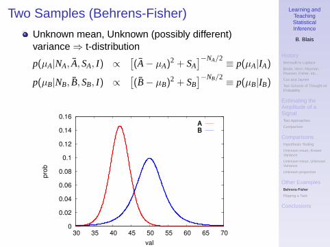
Two Samples (Behrens-Fisher)
Unknown mean, Unknown (possibly different)variance ⇒ t-distribution
p(µA|NA, A, SA, I) ∝[(A− µA)2 + SA
]−NA/2 ≡ p(µA|IA)
p(µB|NB, B, SB, I) ∝[(B− µB)2 + SB
]−NB/2 ≡ p(µB|IB)
0
0.02
0.04
0.06
0.08
0.1
0.12
0.14
0.16
30 35 40 45 50 55 60 65 70
prob
val
ABAB
Learning andTeachingStatisticalInference
B. Blais
HistoryBernoulli to Laplace
Boole, Venn, Neyman,Pearson, Fisher, etc. . .
Cox and Jaynes
Two Schools of Thought onProbability
Estimating theAmplitude of aSignalTwo Approaches
Comparison
ComparisonsHypothesis Testing
Unknown mean, KnownVariance
Unknown mean, UnknownVariance
Unknown proportion
Other ExamplesBehrens-Fisher
Flipping a Tack
Conclusions
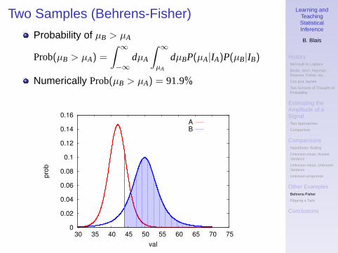
Two Samples (Behrens-Fisher)
Probability of µB > µA
Prob(µB > µA) =
∫ ∞−∞
dµA
∫ ∞µA
dµBP(µA|IA)P(µB|IB)
Numerically Prob(µB > µA) = 91.9%
0
0.02
0.04
0.06
0.08
0.1
0.12
0.14
0.16
30 35 40 45 50 55 60 65 70 75
prob
val
AB
Learning andTeachingStatisticalInference
B. Blais
HistoryBernoulli to Laplace
Boole, Venn, Neyman,Pearson, Fisher, etc. . .
Cox and Jaynes
Two Schools of Thought onProbability
Estimating theAmplitude of aSignalTwo Approaches
Comparison
ComparisonsHypothesis Testing
Unknown mean, KnownVariance
Unknown mean, UnknownVariance
Unknown proportion
Other ExamplesBehrens-Fisher
Flipping a Tack
Conclusions
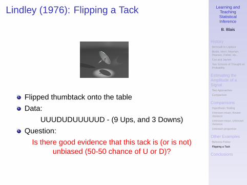
Lindley (1976): Flipping a Tack
Flipped thumbtack onto the table
Data:
UUUDUDUUUUUD - (9 Ups, and 3 Downs)
Question:
Is there good evidence that this tack is (or is not)unbiased (50-50 chance of U or D)?
Learning andTeachingStatisticalInference
B. Blais
HistoryBernoulli to Laplace
Boole, Venn, Neyman,Pearson, Fisher, etc. . .
Cox and Jaynes
Two Schools of Thought onProbability
Estimating theAmplitude of aSignalTwo Approaches
Comparison
ComparisonsHypothesis Testing
Unknown mean, KnownVariance
Unknown mean, UnknownVariance
Unknown proportion
Other ExamplesBehrens-Fisher
Flipping a Tack
Conclusions
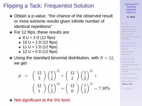
Flipping a Tack: Frequentist Solution
Obtain a p-value: “the chance of the observed resultor more extreme results given infinite number ofidentical repetitions”For 12 flips, these results are
9 U + 3 D (12 flips)10 U + 2 D (12 flips)11 U + 1 D (12 flips)12 U + 0 D (12 flips)
Using the standard binomial distribution, with N = 12,we get
p =
(123
)(12
)12
+
(122
)(12
)12
+(121
)(12
)12
+
(120
)(12
)12
= 7.30%
Not significant at the 5% level
Learning andTeachingStatisticalInference
B. Blais
HistoryBernoulli to Laplace
Boole, Venn, Neyman,Pearson, Fisher, etc. . .
Cox and Jaynes
Two Schools of Thought onProbability
Estimating theAmplitude of aSignalTwo Approaches
Comparison
ComparisonsHypothesis Testing
Unknown mean, KnownVariance
Unknown mean, UnknownVariance
Unknown proportion
Other ExamplesBehrens-Fisher
Flipping a Tack
Conclusions
Frequentist Solution
. . . BUT. . .

Learning andTeachingStatisticalInference
B. Blais
HistoryBernoulli to Laplace
Boole, Venn, Neyman,Pearson, Fisher, etc. . .
Cox and Jaynes
Two Schools of Thought onProbability
Estimating theAmplitude of aSignalTwo Approaches
Comparison
ComparisonsHypothesis Testing
Unknown mean, KnownVariance
Unknown mean, UnknownVariance
Unknown proportion
Other ExamplesBehrens-Fisher
Flipping a Tack
Conclusions
Flipping a Tack: Frequentist Solution
What if the experimenter decided to stop measuringwhen he reached 3 Down?For 3D (3 Down), results at least as extreme are
9 U + 3 D (12 flips)10 U + 3 D (13 flips)11 U + 3 D (14 flips)12 U + 3 D (15 flips)13 U + 3 D (16 flips)...
Using the negative binomial distribution, with D = 3,we get
p =
(12− 13− 1
)(12
)12
+
(13− 13− 1
)(12
)13
+(14− 13− 1
)(12
)14
+ · · · = 3.27%
Is significant at the 5% level
Learning andTeachingStatisticalInference
B. Blais
HistoryBernoulli to Laplace
Boole, Venn, Neyman,Pearson, Fisher, etc. . .
Cox and Jaynes
Two Schools of Thought onProbability
Estimating theAmplitude of aSignalTwo Approaches
Comparison
ComparisonsHypothesis Testing
Unknown mean, KnownVariance
Unknown mean, UnknownVariance
Unknown proportion
Other ExamplesBehrens-Fisher
Flipping a Tack
Conclusions
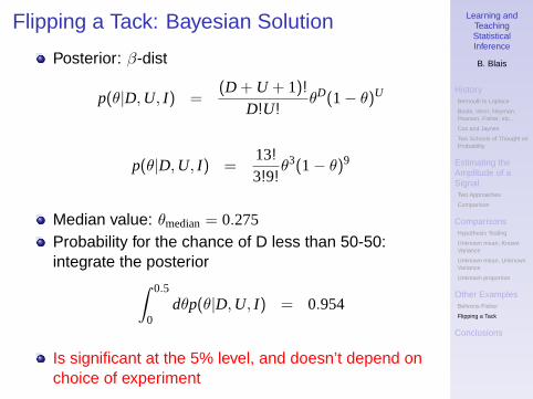
Flipping a Tack: Bayesian Solution
Posterior: β-dist
p(θ|D, U, I) =(D + U + 1)!
D!U!θD(1− θ)U
p(θ|D, U, I) =13!3!9!
θ3(1− θ)9
Median value: θmedian= 0.275Probability for the chance of D less than 50-50:integrate the posterior∫ 0.5
0dθp(θ|D, U, I) = 0.954
Is significant at the 5% level, and doesn’t depend onchoice of experiment
Learning andTeachingStatisticalInference
B. Blais
HistoryBernoulli to Laplace
Boole, Venn, Neyman,Pearson, Fisher, etc. . .
Cox and Jaynes
Two Schools of Thought onProbability
Estimating theAmplitude of aSignalTwo Approaches
Comparison
ComparisonsHypothesis Testing
Unknown mean, KnownVariance
Unknown mean, UnknownVariance
Unknown proportion
Other ExamplesBehrens-Fisher
Flipping a Tack
Conclusions
Conclusions
Two Schools of Thought on ProbabilityBayesianFrequentist
Both schools give identical numerical results to allproblems covered in introductory statistics coursesInterpretation perhaps more straightforward in theBayesian approach
Win-Win: don’t need to modify thecontent/examples/tests/syllabus very much, but yougain a possibly more intuitive perspective
Questions?
Comments?

Learning andTeachingStatisticalInference
B. Blais
Extra ExamplesUnknown µ, Known σ
Unknown µ, Unknown σ
Changing Variables
Difference of Means,δ ≡ µx − µy , knownσx and σy
Simple Linear Regression
Maximum EntropyPriorsKnowledge of N possibilities
Knowledge of Mean
Knowledge of Mean andVariance
Unknown µ, Known σ
(Uniform) Prior
p(µ|σ, I) = p(µ|I) =
{A µmin ≤ µ ≤ µmax
0 otherwise
Likelihood
p(x|µ, σ, I) =N∏
k=1
1√2πσ2
e−(xk−µ)2/2σ2
Posterior
p(µ|x, σ, I) =
√N
2πσ2e−N(x−µ)2/2σ2
Learning andTeachingStatisticalInference
B. Blais
Extra ExamplesUnknown µ, Known σ
Unknown µ, Unknown σ
Changing Variables
Difference of Means,δ ≡ µx − µy , knownσx and σy
Simple Linear Regression
Maximum EntropyPriorsKnowledge of N possibilities
Knowledge of Mean
Knowledge of Mean andVariance
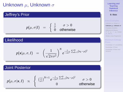
Unknown µ, Unknown σ
Jeffrey’s Prior
p(µ, σ|I) =
{ 1σ σ > 00 otherwise
Likelihood
p(x|µ, σ, I) =
(1√
2πσ2
)N
e1
−2σ2
PNk=1(xk−µ)2
Joint Posterior
p(µ, σ|x, I) ∝
{ (1σ
)N+1e
1−2σ2
PNk=1(xk−µ)2
σ > 00 otherwise

Learning andTeachingStatisticalInference
B. Blais
Extra ExamplesUnknown µ, Known σ
Unknown µ, Unknown σ
Changing Variables
Difference of Means,δ ≡ µx − µy , knownσx and σy
Simple Linear Regression
Maximum EntropyPriorsKnowledge of N possibilities
Knowledge of Mean
Knowledge of Mean andVariance
Unknown µ, Unknown σ, continued. . .
Joint Posterior
p(µ, σ|x, I) ∝
{ (1σ
)N+1e
1−2σ2
PNk=1(xk−µ)2
σ > 00 otherwise
Posterior for µ: t-dist
p(µ|x, I) =
∫ ∞0
p(µ, σ|x, I)dσ
∝[N(x− µ)2 + V
]−N/2
Posterior for σ: χ2-dist
p(σ|x, I) ∝ 1σN e−V/2σ2
Learning andTeachingStatisticalInference
B. Blais
Extra ExamplesUnknown µ, Known σ
Unknown µ, Unknown σ
Changing Variables
Difference of Means,δ ≡ µx − µy , knownσx and σy
Simple Linear Regression
Maximum EntropyPriorsKnowledge of N possibilities
Knowledge of Mean
Knowledge of Mean andVariance
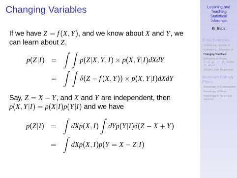
Changing Variables
If we have Z = f (X, Y), and we know about X and Y, wecan learn about Z.
p(Z|I) =
∫ ∫p(Z|X, Y, I)× p(X, Y|I)dXdY
=
∫ ∫δ(Z− f (X, Y))× p(X, Y|I)dXdY
Say, Z = X− Y, and X and Y are independent, thenp(X, Y|I) = p(X|I)p(Y|I) and we have
p(Z|I) =
∫dXp(X, I)
∫dYp(Y|I)δ(Z− X + Y)
=
∫dXp(X, I)p(Y = X− Z|I)

Learning andTeachingStatisticalInference
B. Blais
Extra ExamplesUnknown µ, Known σ
Unknown µ, Unknown σ
Changing Variables
Difference of Means,δ ≡ µx − µy , knownσx and σy
Simple Linear Regression
Maximum EntropyPriorsKnowledge of N possibilities
Knowledge of Mean
Knowledge of Mean andVariance
Difference of Means, δ ≡ µx− µy, known σx
and σy
Posteriors
p(µx|x, σx, I) =
√n
2πσ2x
e−n(x−µx)2/2σ2x
p(µy|y, σy, I) =
√m
2πσ2y
e−n(y−µy)2/2σ2y
Change of Variables
p(δ|x, y, σx, σy, I) =
√nm
2πσxσy
∫dµye
−n(x−δ−µy)2/2σ2x e−m(y−µy)2/2σ2
y
Posterior
µδ ≡ µx− µy , σδ ≡σ2
x
n+
σ2y
m
p(δ|x, y, σx, σy, I) =1√
2πσ2δ
e−(δ−µδ)2/2σ2δ
Learning andTeachingStatisticalInference
B. Blais
Extra ExamplesUnknown µ, Known σ
Unknown µ, Unknown σ
Changing Variables
Difference of Means,δ ≡ µx − µy , knownσx and σy
Simple Linear Regression
Maximum EntropyPriorsKnowledge of N possibilities
Knowledge of Mean
Knowledge of Mean andVariance
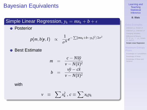
Bayesian Equivalents
Simple Linear Regression, yk = mxk + b + ε
Posterior
p(m, b|y, I) ∝ 1σN e−
P(mxk+b−yk)
2/2σ2
Best Estimate
m =c− Nxy
v− N(x)2
b =vy− cx
v− N(x)2
with
v ≡∑
x2k , c≡
∑xkyk
Learning andTeachingStatisticalInference
B. Blais
Extra ExamplesUnknown µ, Known σ
Unknown µ, Unknown σ
Changing Variables
Difference of Means,δ ≡ µx − µy , knownσx and σy
Simple Linear Regression
Maximum EntropyPriorsKnowledge of N possibilities
Knowledge of Mean
Knowledge of Mean andVariance
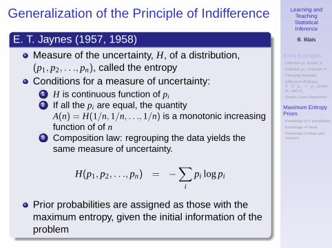
Generalization of the Principle of Indifference
E. T. Jaynes (1957, 1958)Measure of the uncertainty, H, of a distribution,(p1, p2, . . ., pn), called the entropyConditions for a measure of uncertainty:
1 H is continuous function of pi2 If all the pi are equal, the quantity
A(n) = H(1/n, 1/n, . . ., 1/n) is a monotonic increasingfunction of of n
3 Composition law: regrouping the data yields thesame measure of uncertainty.
H(p1, p2, . . ., pn) = −∑
i
pi logpi
Prior probabilities are assigned as those with themaximum entropy, given the initial information of theproblem
Learning andTeachingStatisticalInference
B. Blais
Extra ExamplesUnknown µ, Known σ
Unknown µ, Unknown σ
Changing Variables
Difference of Means,δ ≡ µx − µy , knownσx and σy
Simple Linear Regression
Maximum EntropyPriorsKnowledge of N possibilities
Knowledge of Mean
Knowledge of Mean andVariance
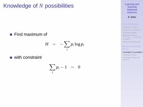
Knowledge of N possibilities
Find maximum of
H = −∑
i
pi logpi
with constraint ∑i
pi − 1 = 0

Learning andTeachingStatisticalInference
B. Blais
Extra ExamplesUnknown µ, Known σ
Unknown µ, Unknown σ
Changing Variables
Difference of Means,δ ≡ µx − µy , knownσx and σy
Simple Linear Regression
Maximum EntropyPriorsKnowledge of N possibilities
Knowledge of Mean
Knowledge of Mean andVariance
Knowledge of N possibilities
Find maximum of
Q = −∑
i
pi logpi + λo
(1−
∑i
pi
)
setting ∂Q/∂pj = 0 we get
pj = e−(1+λo) = (const)
normalizing we get
pj =1N
Learning andTeachingStatisticalInference
B. Blais
Extra ExamplesUnknown µ, Known σ
Unknown µ, Unknown σ
Changing Variables
Difference of Means,δ ≡ µx − µy , knownσx and σy
Simple Linear Regression
Maximum EntropyPriorsKnowledge of N possibilities
Knowledge of Mean
Knowledge of Mean andVariance
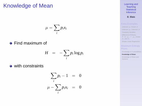
Knowledge of Mean
µ =∑
i
pixi
Find maximum of
H = −∑
i
pi logpi
with constraints ∑i
pi − 1 = 0
µ−∑
i
pixi = 0
Learning andTeachingStatisticalInference
B. Blais
Extra ExamplesUnknown µ, Known σ
Unknown µ, Unknown σ
Changing Variables
Difference of Means,δ ≡ µx − µy , knownσx and σy
Simple Linear Regression
Maximum EntropyPriorsKnowledge of N possibilities
Knowledge of Mean
Knowledge of Mean andVariance
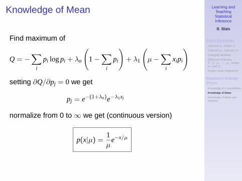
Knowledge of Mean
Find maximum of
Q = −∑
i
pi logpi + λo
(1−
∑i
pi
)+ λ1
(µ−
∑i
xipi
)
setting ∂Q/∂pj = 0 we get
pj = e−(1+λo)e−λ1xj
normalize from 0 to ∞ we get (continuous version)
p(x|µ) =1µ
e−x/µ
Learning andTeachingStatisticalInference
B. Blais
Extra ExamplesUnknown µ, Known σ
Unknown µ, Unknown σ
Changing Variables
Difference of Means,δ ≡ µx − µy , knownσx and σy
Simple Linear Regression
Maximum EntropyPriorsKnowledge of N possibilities
Knowledge of Mean
Knowledge of Mean andVariance
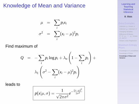
Knowledge of Mean and Variance
µ =∑
i
pixi
σ2 =∑
i
(xi − µ)2pi
Find maximum of
Q = −∑
i
pi logpi + λo
(1−
∑i
pi
)+
λ1
(σ2−
∑i
(xi − µ)2pi
)
leads to
p(x|µ, σ) =1√
2πσ2e−
(x−µ)2
2σ2