Chapter 16spielman/PAPERS/SGTChapter.pdf · Spectral Graph Theory 3 16.3 The matrices associated...

Chapter 16

Spectral Graph Theory

Daniel Spielman

Yale University

16.1 Introduction . . . . . . . . . . . . . . . . . . . . . . . . . . . . . . . . . . . . . . . . . . . . . . . . . . . . . . . . . . . . . . . 116.2 Preliminaries . . . . . . . . . . . . . . . . . . . . . . . . . . . . . . . . . . . . . . . . . . . . . . . . . . . . . . . . . . . . . . 216.3 The matrices associated with a graph . . . . . . . . . . . . . . . . . . . . . . . . . . . . . . . . . . . . 2

16.3.1 Operators on the vertices . . . . . . . . . . . . . . . . . . . . . . . . . . . . . . . . . . . . . . . . . 316.3.2 The Laplacian Quadratic Form . . . . . . . . . . . . . . . . . . . . . . . . . . . . . . . . . . . 416.3.3 The Normalized Laplacian . . . . . . . . . . . . . . . . . . . . . . . . . . . . . . . . . . . . . . . . 516.3.4 Naming the Eigenvalues . . . . . . . . . . . . . . . . . . . . . . . . . . . . . . . . . . . . . . . . . . . 5

16.4 Some Examples . . . . . . . . . . . . . . . . . . . . . . . . . . . . . . . . . . . . . . . . . . . . . . . . . . . . . . . . . . . 616.5 The Role of the Courant-Fischer Theorem . . . . . . . . . . . . . . . . . . . . . . . . . . . . . . . 9

16.5.1 Low-Rank Approximations . . . . . . . . . . . . . . . . . . . . . . . . . . . . . . . . . . . . . . . . 916.6 Elementary Facts . . . . . . . . . . . . . . . . . . . . . . . . . . . . . . . . . . . . . . . . . . . . . . . . . . . . . . . . . . 1016.7 Spectral Graph Drawing . . . . . . . . . . . . . . . . . . . . . . . . . . . . . . . . . . . . . . . . . . . . . . . . . . 1116.8 Algebraic Connectivity and Graph Partitioning . . . . . . . . . . . . . . . . . . . . . . . . . . 11

16.8.1 Convergence of Random Walks . . . . . . . . . . . . . . . . . . . . . . . . . . . . . . . . . . . 1416.8.2 Expander Graphs . . . . . . . . . . . . . . . . . . . . . . . . . . . . . . . . . . . . . . . . . . . . . . . . . 1416.8.3 Ramanujan Graphs . . . . . . . . . . . . . . . . . . . . . . . . . . . . . . . . . . . . . . . . . . . . . . . . 1616.8.4 Bounding !2 . . . . . . . . . . . . . . . . . . . . . . . . . . . . . . . . . . . . . . . . . . . . . . . . . . . . . . . 16

16.9 Coloring and Independent Sets . . . . . . . . . . . . . . . . . . . . . . . . . . . . . . . . . . . . . . . . . . . 1716.10Perturbation Theory and Random Graphs . . . . . . . . . . . . . . . . . . . . . . . . . . . . . . . 1816.11Relative Spectral Graph Theory . . . . . . . . . . . . . . . . . . . . . . . . . . . . . . . . . . . . . . . . . . 2016.12Directed Graphs . . . . . . . . . . . . . . . . . . . . . . . . . . . . . . . . . . . . . . . . . . . . . . . . . . . . . . . . . . . 2116.13Concluding Remarks . . . . . . . . . . . . . . . . . . . . . . . . . . . . . . . . . . . . . . . . . . . . . . . . . . . . . . 22

Bibliography . . . . . . . . . . . . . . . . . . . . . . . . . . . . . . . . . . . . . . . . . . . . . . . . . . . . . . . . . . . . . . . 23

16.1 Introduction

Spectral graph theory is the study and exploration of graphs throughthe eigenvalues and eigenvectors of matrices naturally associated with thosegraphs. It is intuitively related to attempts to understand graphs through thesimulation of processes on graphs and through the consideration of physicalsystems related to graphs. Spectral graph theory provides many useful algo-rithms, as well as some that can be rigorously analyzed. We begin this chapterby providing intuition as to why interesting properties of graphs should berevealed by these eigenvalues and eigenvectors. We then survey a few appli-cations of spectral graph theory.

1

2 Combinatorial Scientific Computing

The figures in this chapter are accompanied by the Matlab code used togenerate them.

16.2 Preliminaries

We ordinarily view an undirected graph1 G as a pair (V,E), where Vdenotes its set of vertices and E denotes its set of edges. Each edge in E is anunordered pair of vertices, with the edge connecting distinct vertices a and bwritten as (a, b). A weighted graph is a graph in which a weight (typically areal number) has been assigned to every edge. We denote a weighted graphby a triple (V,E,w), where (V,E) is the associated unweighted graph, and wis a function from E to the real numbers. We restrict our attention to weightfunctions w that are strictly positive. We reserve the letter n for the numberof vertices in a graph. The degree of a vertex in an unweighted graph is thenumber of edges in which it is involved. We say that a graph is regular if everyvertex has the same degree, and d-regular if that degree is d.

We denote vectors by bold letters, and denote the ith component of a vectorx by x (i). Similarly, we denote the entry in the ith row and jth column of amatrix M by M(i, j).

If we are going to discuss the eigenvectors and eigenvalues of a matrix M ,we should be sure that they exist. When considering undirected graphs, mostof the matrices we consider are symmetric, and thus they have an orthonormalbasis of eigenvectors and n eigenvalues, counted with multiplicity. The othermatrices we associate with undirected graphs are similar to symmetric ma-trices, and thus also have n eigenvalues, counted by multiplicity, and possessa basis of eigenvectors. In particular, these matrices are of the form MD!1,where M is symmetric and D is a non-singular diagonal matrix. In this case,D!1/2MD!1/2 is symmetric, and we have

D!1/2MD!1/2v i = !iv i =! MD!1(D1/2v i) = !i

!

D1/2v i

"

.

So, if v1, . . . , vn form an orthonormal basis of eigenvectors of D!1/2MD!1/2,then we obtain a basis (not necessarily orthonormal) of eigenvectors of MD!1

by multiplying these vectors by D1/2. Moreover, these matrices have the sameeigenvalues.

The matrices we associate with directed graphs will not necessarily bediagonalizable.

1Strictly speaking, we are considering simple graphs. These are the graphs in which alledges go between distinct vertices and in which there can be at most one edge between agiven pair of vertices. Graphs that have multiple-edges or self-loops are often called multi-graphs.

Spectral Graph Theory 3

16.3 The matrices associated with a graph

Many di!erent matrices arise in the field of Spectral Graph Theory. In thissection we introduce the most prominent.

16.3.1 Operators on the vertices

Eigenvalues and eigenvectors are used to understand what happens whenone repeatedly applies an operator to a vector. If A is an n-by-nmatrix havinga basis of right-eigenvectors v1, . . . , vn with

Av i = !iv i,

then we can use these eigenvectors to understand the impact of multiplying avector x by A. We first express x in the eigenbasis

x =#

i

civ i

and then compute

Akx =#

i

ciAkv i =

#

i

ci!ki v i.

If we have an operator that is naturally associated with a graph G, thenproperties of this operator, and therefore of the graph, will be revealed by itseigenvalues and eigenvectors. The first operator one typically associates witha graph G is its adjacency operator, realized by its adjacency matrix AG anddefined by

AG(i, j) =

$

1 if (i, j) " E

0 otherwise.

To understand spectral graph theory, one must view vectors x " IRn asfunctions from the vertices to the Reals. That is, they should be understoodas vectors in IRV . When we apply the adjacency operator to such a function,the resulting value at a vertex a is the sum of the values of the function xover all neighbors b of a:

(AGx ) (a) =#

b:(a,b)"E

x (b).

This is very close to one of the most natural operators on a graph: thedi!usion operator. Intuitively, the di!usion operator represents a process inwhich “stu!” or “mass” moves from vertices to their neighbors. As massshould be conserved, the mass at a given vertex is distributed evenly among


its neighbors. Formally, we define the degree of a vertex a to be the numberof edges in which it participates. We naturally encode this in a vector, labeledd :

d (a) = |{b : (a, b) " E}| ,

where we write |S| to indicate the number of elements in a set S. We thendefine the degree matrix DG by

DG(a, b) =

$

d(a) if a = b

0 otherwise.

The di!usion matrix of G, also called the walk matrix of G, is then given by

WGdef= AGD

!1G . (16.1)

It acts on a vector x by

(WGx ) (a) =#

b:(a,b)"E

x (b)/d(b).

This matrix is called the walk matrix of G because it encodes the dynamicsof a random walk on G. Recall that a random walk is a process that beginsat some vertex, then moves to a random neighbor of that vertex, and then arandom neighbor of that vertex, and so on. The walk matrix is used to studythe evolution of the probability distribution of a random walk. If p " IRn

is a probability distribution on the vertices, then WGp is the probabilitydistribution obtained by selecting a vertex according to p , and then selectinga random neighbor of that vertex. As the eigenvalues and eigenvectors of WG

provide information about the behavior of a random walk on G, they alsoprovide information about the graph.

Of course, adjacency and walk matrices can also be defined for weightedgraphs G = (V,E,w). For a weighted graph G, we define

AG(a, b) =

$

w(a, b) if (a, b) " E

0 otherwise.

When dealing with weighted graphs, we distinguish between the weighted de-gree of a vertex, which is defined to be the sum of the weights of its attachededges, and the combinatorial degree of a vertex, which is the number of suchedges. We reserve the vector d for the weighted degree, so

d(a) =#

b:(a,b)"E

w(a, b).

The random walk on a weighted graph moves from a vertex a to a neighbor bwith probability proportional to w(a, b), so we still define its walk matrix byequation (16.1).


16.3.2 The Laplacian Quadratic Form

Matrices and spectral theory also arise in the study of quadratic forms.The most natural quadratic form to associate with a graph is the Laplacian,which is given by

xTLGx =#

(a,b)"E

w(a, b)(x (a)# x (b))2. (16.2)

This form measures the smoothness of the function x . It will be small if thefunction x does not jump too much over any edge. The matrix defining thisform is the Laplacian matrix of the graph G,

LGdef= DG #AG.

The Laplacian matrices of weighted graphs arise in many applications.For example, they appear when applying the certain discretization schemes tosolve Laplace’s equation with Neumann boundary conditions. They also arisewhen modeling networks of springs or resistors. As resistor networks provide avery useful physical model for graphs, we explain the analogy in more detail.We associate an edge of weight w with a resistor of resistance 1/w, sincehigher weight corresponds to higher connectivity which corresponds to lessresistance.

When we inject and withdraw current from a network of resistors, we leti ext(a) denote the amount of current we inject into node a. If this quantity isnegative then we are removing current. As electrical flow is a potential flow,there is a vector v " IRV so that the amount of current that flows across edge(a, b) is

i(a, b) = (v(a)# v (b)) /r(a, b),

where r(a, b) is the resistance of edge (a, b). The Laplacian matrix provides asystem of linear equations that may be used to solve for v when given i ext:

i ext = LGv . (16.3)

We refer the reader to [1] or [2] for more information about the connectionsbetween resistor networks and graphs.

16.3.3 The Normalized Laplacian

When studying random walks on a graph, it often proves useful to nor-malize the Laplacian by its degrees. The normalized Laplacian of G is definedby

NG = D!1/2G LGD

!1/2G = I #D!1/2

G AGD!1/2G .

It should be clear that normalized Laplacian is closely related to the walkmatrix of a graph. Chung’s monograph on spectral graph theory focuses onthe normalized Laplacian [3].


16.3.4 Naming the Eigenvalues

When the graph G is understood, we will always let

"1 $ "2 $ · · · $ "n

denote the eigenvalues of the adjacency matrix. We order the eigenvalues ofthe Laplacian in the other direction:

0 = !1 % !2 % · · · % !n.

We will always let0 = #1 % #2 % · · · % #n

denote the eigenvalues of the normalized Laplacian. Even though $ is not aGreek variant of w, we use

1 = $1 $ $2 $ · · · $ $n

to denote the eigenvalues of the walk matrix. It is easy to show that $i = 1##i.For graphs in which every vertex has the same weighted degree the degree

matrix is a multiple of the identity; so, AG and LG have the same eigenvectors.For graphs that are not regular, the eigenvectors of AG and LG can behavevery di!erently.

16.4 Some Examples

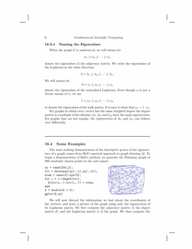
The most striking demonstration of the descriptive power of the eigenvec-tors of a graph comes from Hall’s spectral approach to graph drawing [4]. Tobegin a demonstration of Hall’s method, we generate the Delaunay graph of200 randomly chosen points in the unit square.

xy = rand(200,2);tri = delaunay(xy(:,1),xy(:,2));elem = ones(3)-eye(3);for i = 1:length(tri),A(tri(i,:),tri(i,:)) = elem;

endA = double(A > 0);gplot(A,xy)

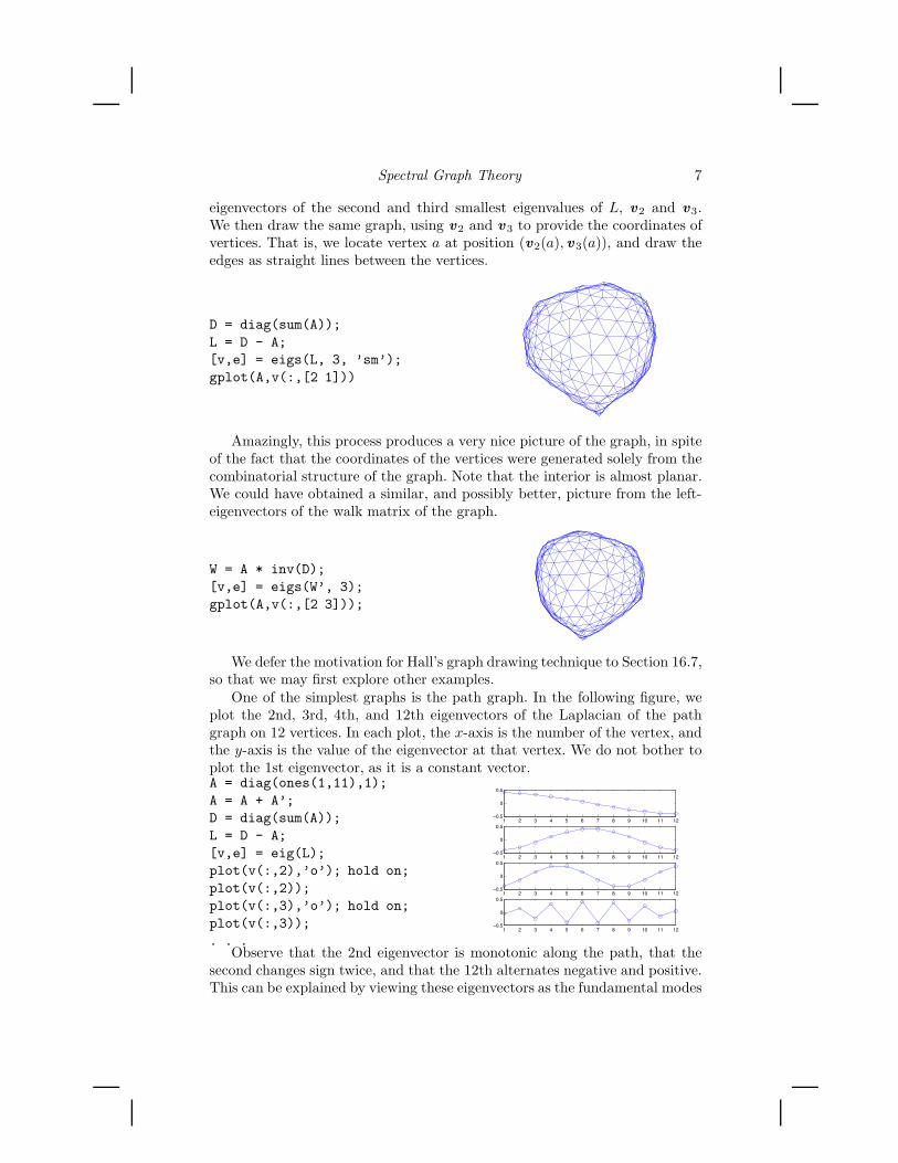
We will now discard the information we had about the coordinates ofthe vertices, and draw a picture of the graph using only the eigenvectors ofits Laplacian matrix. We first compute the adjacency matrix A, the degreematrix D, and the Laplacian matrix L of the graph. We then compute the


eigenvectors of the second and third smallest eigenvalues of L, v2 and v3.We then draw the same graph, using v2 and v3 to provide the coordinates ofvertices. That is, we locate vertex a at position (v2(a), v3(a)), and draw theedges as straight lines between the vertices.

D = diag(sum(A));L = D - A;[v,e] = eigs(L, 3, ’sm’);gplot(A,v(:,[2 1]))

Amazingly, this process produces a very nice picture of the graph, in spiteof the fact that the coordinates of the vertices were generated solely from thecombinatorial structure of the graph. Note that the interior is almost planar.We could have obtained a similar, and possibly better, picture from the left-eigenvectors of the walk matrix of the graph.

W = A * inv(D);[v,e] = eigs(W’, 3);gplot(A,v(:,[2 3]));

We defer the motivation for Hall’s graph drawing technique to Section 16.7,so that we may first explore other examples.

One of the simplest graphs is the path graph. In the following figure, weplot the 2nd, 3rd, 4th, and 12th eigenvectors of the Laplacian of the pathgraph on 12 vertices. In each plot, the x-axis is the number of the vertex, andthe y-axis is the value of the eigenvector at that vertex. We do not bother toplot the 1st eigenvector, as it is a constant vector.A = diag(ones(1,11),1);A = A + A’;D = diag(sum(A));L = D - A;[v,e] = eig(L);plot(v(:,2),’o’); hold on;plot(v(:,2));plot(v(:,3),’o’); hold on;plot(v(:,3));. . .

1 2 3 4 5 6 7 8 9 10 11 12−0.5

0

0.5

1 2 3 4 5 6 7 8 9 10 11 12−0.5

0

0.5

1 2 3 4 5 6 7 8 9 10 11 12−0.5

0

0.5

1 2 3 4 5 6 7 8 9 10 11 12−0.5

0

0.5

Observe that the 2nd eigenvector is monotonic along the path, that thesecond changes sign twice, and that the 12th alternates negative and positive.This can be explained by viewing these eigenvectors as the fundamental modes


of vibration of a discretization of a string. We recommend [5] for a formaltreatment.

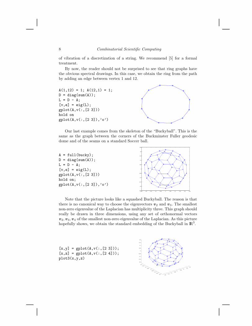
By now, the reader should not be surprised to see that ring graphs havethe obvious spectral drawings. In this case, we obtain the ring from the pathby adding an edge between vertex 1 and 12.

A(1,12) = 1; A(12,1) = 1;D = diag(sum(A));L = D - A;[v,e] = eig(L);gplot(A,v(:,[2 3]))hold ongplot(A,v(:,[2 3]),’o’)

Our last example comes from the skeleton of the “Buckyball”. This is thesame as the graph between the corners of the Buckminster Fuller geodesicdome and of the seams on a standard Soccer ball.

A = full(bucky);D = diag(sum(A));L = D - A;[v,e] = eig(L);gplot(A,v(:,[2 3]))hold on;gplot(A,v(:,[2 3]),’o’)

−0.25 −0.2 −0.15 −0.1 −0.05 0 0.05 0.1 0.15 0.2 0.25−0.25

−0.2

−0.15

−0.1

−0.05

0

0.05

0.1

0.15

0.2

0.25

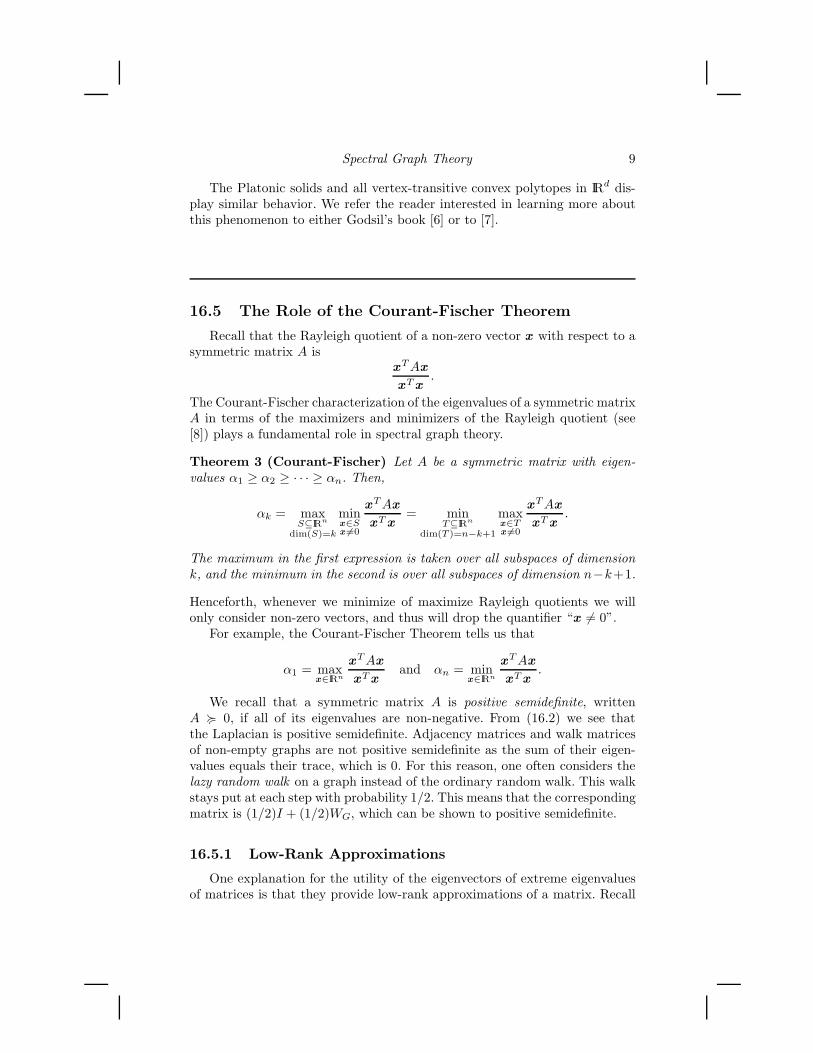
Note that the picture looks like a squashed Buckyball. The reason is thatthere is no canonical way to choose the eigenvectors v2 and v3. The smallestnon-zero eigenvalue of the Laplacian has multiplicity three. This graph shouldreally be drawn in three dimensions, using any set of orthonormal vectorsv2, v3, v4 of the smallest non-zero eigenvalue of the Laplacian. As this picturehopefully shows, we obtain the standard embedding of the Buckyball in IR3.

[x,y] = gplot(A,v(:,[2 3]));[x,z] = gplot(A,v(:,[2 4]));plot3(x,y,z)

−0.2−0.15

−0.1−0.05

00.05

0.10.15

0.2

−0.2−0.15

−0.1−0.05

00.05

0.10.15

0.2

−0.2

−0.15

−0.1

−0.05

0

0.05

0.1

0.15

0.2


The Platonic solids and all vertex-transitive convex polytopes in IRd dis-play similar behavior. We refer the reader interested in learning more aboutthis phenomenon to either Godsil’s book [6] or to [7].

16.5 The Role of the Courant-Fischer Theorem

Recall that the Rayleigh quotient of a non-zero vector x with respect to asymmetric matrix A is

xTAx

xTx.

The Courant-Fischer characterization of the eigenvalues of a symmetric matrixA in terms of the maximizers and minimizers of the Rayleigh quotient (see[8]) plays a fundamental role in spectral graph theory.

Theorem 3 (Courant-Fischer) Let A be a symmetric matrix with eigen-values "1 $ "2 $ · · · $ "n. Then,

"k = maxS#IRn

dim(S)=k

minx"Sx $=0

xTAx

xTx= min

T#IRn

dim(T )=n!k+1

maxx"Tx $=0

xTAx

xTx.

The maximum in the first expression is taken over all subspaces of dimensionk, and the minimum in the second is over all subspaces of dimension n#k+1.

Henceforth, whenever we minimize of maximize Rayleigh quotients we willonly consider non-zero vectors, and thus will drop the quantifier “x &= 0”.

For example, the Courant-Fischer Theorem tells us that

"1 = maxx"IRn

xTAx

xTxand "n = min

x"IRn

xTAx

xTx.

We recall that a symmetric matrix A is positive semidefinite, writtenA ! 0, if all of its eigenvalues are non-negative. From (16.2) we see thatthe Laplacian is positive semidefinite. Adjacency matrices and walk matricesof non-empty graphs are not positive semidefinite as the sum of their eigen-values equals their trace, which is 0. For this reason, one often considers thelazy random walk on a graph instead of the ordinary random walk. This walkstays put at each step with probability 1/2. This means that the correspondingmatrix is (1/2)I + (1/2)WG, which can be shown to positive semidefinite.

16.5.1 Low-Rank Approximations

One explanation for the utility of the eigenvectors of extreme eigenvaluesof matrices is that they provide low-rank approximations of a matrix. Recall


that if A is a symmetric matrix with eigenvalues "1 $ "2 $ · · · $ "n and acorresponding orthonormal basis of column eigenvectors v1, . . . , vn, then

A =#

i

"iv ivTi .

We can measure how well a matrix B approximates a matrix A by either theoperator norm 'A#B' or the Frobenius norm 'A#B'F , where we recall

'M' def= max

x

'Mx''x' and 'M'F

def=

%

#

i,j

M(i, j)2.

Using the Courant-Fischer Theorem, one can prove that for every k, thebest approximation of A by a rank-k matrix is given by summing the terms"iv ivT

i over the k values of i for which |"i| is largest. This holds regardless ofwhether we measure the quality of approximation in the operator or Frobeniusnorm.

When the di!erence between A and its best rank-k approximation is small,it explains why the eigenvectors of the largest k eigenvalues ofA should providea lot of information about A. However, one must be careful when applyingthis intuition as the analogous eigenvectors of the Laplacian correspond to issmallest eigenvalues. Perhpas the best way to explain the utility of these smalleigenvectors is to observe that they provide the best low-rank approximationof the pseudoinverse of the Laplacian.

16.6 Elementary Facts

We list some elementary facts about the extreme eigenvalues of the Lapla-cian and adjacency matrices. We recommend deriving proofs yourself, or con-sulting the suggested references.

1. The all-1s vector is always an eigenvector of LG of eigenvalue 0.

2. The largest eigenvalue of the adjacency matrix is at least the averagedegree of a vertex of G and at most the maximum degree of a vertex ofG (see [9] or [10, Section 3.2]).

3. If G is connected, then "1 > "2 and the eigenvector of "1 may be takento be positive (this follows from the Perron-Frobenius theory; see [11]).

4. The all-1s vector is an eigenvector of AG with eigenvalue "1 if and onlyif G is an "1-regular graph.

5. The multiplicity of 0 as an eigenvalue of LG is equal to the number ofconnected components of LG.


6. The largest eigenvalue of LG is at most twice the maximum degree of avertex in G.

7. "n = #"1 if and only if G is bipartite (see [12], or [10, Theorem 3.4]).

16.7 Spectral Graph Drawing

We can now explain the motivation behind Hall’s spectral graph drawingtechnique [4]. Hall first considered the problem of assigning a real numberx (a) to each vertex a so that (x (a) # x (b))2 is small for most edges (a, b).This led him to consider the problem of minimizing (16.2). So as to avoidthe degenerate solutions in which every vertex is mapped to zero, or anyother value, he introduces the restriction that x be orthogonal to b1. As theutility of the embedding does not really depend upon its scale, he suggestedthe normalization 'x' = 1. By the Courant-Fischer Theorem, the solution tothe resulting optimization problem is precisely an eigenvector of the second-smallest eigenvalue of the Laplacian.

But, what if we want to assign the vertices to points in IR2? The naturalminimization problem,

minx ,y"IRV

#

(a,b)"E

'(x (a), y(a))# (x (b), y(b))'2

such that#

a

(x (a), y(a)) = (0, 0)

typically results in the degenerate solution x = y = v2. To ensure that the twocoordinates are di!erent, Hall introduced the restriction that x be orthogonalto y . One can use the Courant-Fischer Theorem to show that the optimalsolution is then given by setting x = v2 and y = v3, or by taking a rotationof this solution.

Hall observes that this embedding seems to cluster vertices that are closein the graph, and separate vertices that are far in the graph. For more sophis-ticated approaches to drawing graphs, we refer the reader to Chapter 15.

16.8 Algebraic Connectivity and Graph Partitioning

Many useful ideas in spectral graph theory have arisen from e!orts to findquantitative analogs of qualitative statements. For example, it is easy to show


that !2 > 0 if and only if G is connected. This led Fiedler [13] to label !2

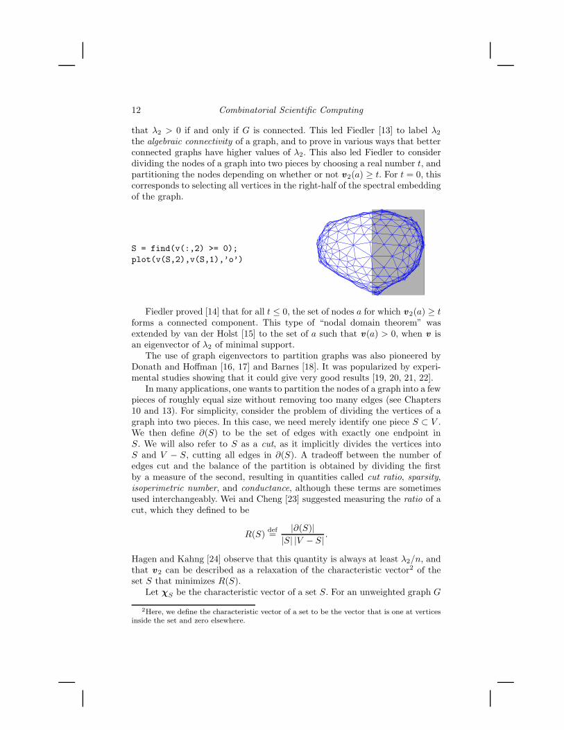
the algebraic connectivity of a graph, and to prove in various ways that betterconnected graphs have higher values of !2. This also led Fiedler to considerdividing the nodes of a graph into two pieces by choosing a real number t, andpartitioning the nodes depending on whether or not v2(a) $ t. For t = 0, thiscorresponds to selecting all vertices in the right-half of the spectral embeddingof the graph.

S = find(v(:,2) >= 0);plot(v(S,2),v(S,1),’o’)

Fiedler proved [14] that for all t % 0, the set of nodes a for which v2(a) $ tforms a connected component. This type of “nodal domain theorem” wasextended by van der Holst [15] to the set of a such that v(a) > 0, when v isan eigenvector of !2 of minimal support.

The use of graph eigenvectors to partition graphs was also pioneered byDonath and Ho!man [16, 17] and Barnes [18]. It was popularized by experi-mental studies showing that it could give very good results [19, 20, 21, 22].

In many applications, one wants to partition the nodes of a graph into a fewpieces of roughly equal size without removing too many edges (see Chapters10 and 13). For simplicity, consider the problem of dividing the vertices of agraph into two pieces. In this case, we need merely identify one piece S ( V .We then define %(S) to be the set of edges with exactly one endpoint inS. We will also refer to S as a cut, as it implicitly divides the vertices intoS and V # S, cutting all edges in %(S). A tradeo! between the number ofedges cut and the balance of the partition is obtained by dividing the firstby a measure of the second, resulting in quantities called cut ratio, sparsity,isoperimetric number, and conductance, although these terms are sometimesused interchangeably. Wei and Cheng [23] suggested measuring the ratio of acut, which they defined to be

R(S)def=

|%(S)||S| |V # S| .

Hagen and Kahng [24] observe that this quantity is always at least !2/n, andthat v2 can be described as a relaxation of the characteristic vector2 of theset S that minimizes R(S).

Let !S be the characteristic vector of a set S. For an unweighted graph G

2Here, we define the characteristic vector of a set to be the vector that is one at verticesinside the set and zero elsewhere.


we have!

TSLG!S = |%(S)| ,

and#

a<b

(!S(a)# !S(b))2 = |S| |V # S| .

So,

R(S) =!

TSLG!S

&

a<b(!S(a)# !S(b))2.

On the other hand, Fiedler [14] proved that

!2 = n minx $=b0

xTLGx&

a<b(x (a)# x (b))2.

If we impose the restriction that x be a zero-one valued vector and thenminimize this last expression, we obtain the characteristic vector of the setof minimum ratio. As we have imposed a constraint on the vector x , theminimum ratio obtained must be larger than !2. Hagen and Kahng make thisobservation, and suggest using v2 to try to find a set of low ratio by choosingsome value t, and setting S = {a : v (a) $ t}.

One may actually prove that the set obtained in this fashion does not haveratio too much worse than the minimum. Statements of this form follow fromdiscrete versions of Cheeger’s inequality [25]. The cleanest version relates tothe the conductance of a set S

&(S)def=

w(%(S))

min(d(S),d(V # S)),

where d(S) denotes the sum of the degrees of the vertices in S and w(%(S))denotes the sum of the weights of the edges in %(S). The conductance of thegraph G is defined by

&G = min%&S&V

&(S).

By a similar relaxation argument, one can show

2&G $ #2.

Sinclair and Jerrum’s discrete version of Cheeger’s inequality [26] says that

#2 % &2G/2.

Moreover, their proof reveals that if v2 is an eigenvector of #2, then thereexists a t so that

&!'

a : d!1/2(a)v2(a) $ t("

%)2#2.

Other discretizations of Cheeger’s inequality were proved around the same


time by a number of researchers. See [27, 28, 29, 30, 31]. We remark thatLawler and Sokal define conductance by

w(%(S))

d(S)d(V # S),

which is proportional to the normalized cut measure

w(%(S))

d(S)+

w(%(V # S))

d(V # S)

popularized by Shi and Malik [21]. The advantage of this later formulation isthat it has an obvious generalization to partitions into more than two pieces.

In general, the eigenvalues and entries of eigenvectors of Laplacian matri-ces will not be rational numbers; so, it is unreasonable to hope to computethem exactly. Mihail [32] proves that an approximation of the second-smallesteigenvector su"ces. While her argument was stated for regular graphs, onecan apply it to irregular, weighted graphs to show that for every vector xorthogonal to d1/2 there exists a t so that

&!'

a : d!1/2(a)x (a) $ t("

%)

2xTNGx

xTx.

While spectral partitioning heuristics are easy to implement, they are nei-ther the most e!ective in practice or in theory. Theoretically better algorithmshave been obtained by linear programming [33] and by semi-definite program-ming [34]. Fast variants of these algorithms may be found in [35, 36, 37, 38, 39].More practical algorithms are discussed in Chapters 10 and 13.

16.8.1 Convergence of Random Walks

If G is a connected, undirected graph, then the largest eigenvalue of WG,$1, has multiplicity 1, equals 1, and has eigenvector d . We may convert thiseigenvector into a probability distribution " by setting

" =d

&

a d(a).

If $n &= #1, then the distribution of every random walk eventually convergesto ". The rate of this convergence is governed by how close max($2,#$n) isto $1. For example, let pt denote the distribution after t steps of a randomwalk that starts at vertex a. Then for every vertex b,

|pt(b)# "(b)| %

%

d(b)

d(a)(1#max($2,#$n))

t .

One intuition behind Cheeger’s inequality is that sets of small conductanceare precisely the obstacles to the convergence of random walks.

For more information about random walks on graphs, we recommend thesurvey of Lovasz [40] and the book by Doyle and Snell [2].


16.8.2 Expander Graphs

Some of the most fascinating graphs are those on which random walksmix quickly and which have high conductance. These are called expandergraphs, and may be defined as the d-regular graphs for which all non-zeroLaplacian eigenvalues are bounded away from zero. In the better expandergraphs, all the Laplacian eigenvalues are close to d. One typically considersinfinite families of such graphs in which d and a lower bound on the distance ofthe non-zero eigenvalues from d remain constant. These are counter-examplesto many naive conjectures about graphs, and should be kept in mind wheneverone is thinking about graphs. They have many amazing properties, and havebeen used throughout Theoretical Computer Science. In addition to playing aprominent role in countless theorems, they are used in the design of pseudo-random generators [41, 42, 43], error-correcting codes [44, 45, 46, 47, 48],fault-tolerant circuits [49] and routing networks [50].

The reason such graphs are called expanders is that all small sets of verticesin these graphs have unusually large numbers of neighbors. That is, theirneighborhoods expand. For S ( V , let N(S) denote the set of vertices thatare neighbors of vertices in S. Tanner [51] provides a lower bound on the sizeof N(S) in bipartite graphs. In general graphs, it becomes the following.

Theorem 4 Let G = (V,E) be a d-regular graph on n vertices and set

' = max

*

1# !2

d,!n

d# 1

+

Then, for all S * V ,

|N(S)| $ |S|'2(1# ") + "

,

where |S| = "n.

The term ' is small when all of the eigenvalues are close to d. Note that when" is much less than '2, the term on the right is approximately |S| /'2, whichcan be much larger than |S|.

An example of the pseudo-random properties of expander graphs is the“Expander Mixing Lemma”. To understand it, consider choosing two subsetsof the vertices, S and T of sizes "n and (n, at random. Let )E(S, T ) denote theset of ordered pairs (a, b) with a " S, b " T and (a, b) " E. The expected sizeof )E(S, T ) is "(dn. This theorem tells us that for every pair of large sets Sand T , the number of such pairs is approximately this quantity. Alternatively,one may view an expander as an approximation of the complete graph. Thefraction of edges in the complete graph going from S to T is "(. The followingtheorem says that the same is approximately true for all su"ciently large setsS and T .

Theorem 5 (Expander Mixing Lemma) Let G = (V,E) be a d-regular


graph and set

' = max

*

1# !2

d,!n

d# 1

+

Then, for every S * V and T * V ,,

,

,

,

,

,

)E(S, T ),

,

,# "(dn

,

,

,% 'dn

-

("# "2)(( # (2),

where |S| = "n and |T | = (n.

This bound is a slight extension by Beigel, Margulis and Spielman [52] of abound originally proved by Alon and Chung [53]. Observe that when " and (are greater than ', the term on the right is less than "(dn. Theorem 4 maybe derived from Theorem 5.

We refer readers who would like to learn more about expander graphs tothe survey of Hoory, Linial and Wigderson [54].

16.8.3 Ramanujan Graphs

Given the importance of !2, we should know how close it can be to d.Nilli [55] shows that it cannot be much closer than 2

)d# 1.

Theorem 6 Let G be an unweighted d-regular graph containing two edges(u0, u1) and (v0, v1) whose vertices are at distance at least 2k + 2 from eachother. Then

!2 % d# 2)d# 1 +

2)d# 1# 1

k + 1.

Amazingly, Margulis [56] and Lubotzky, Phillips and Sarnak [57] haveconstructed infinite families of d-regular graphs, called Ramanujan graphs,for which !2 $ d# 2

)d# 1.

However, this is not the end of the story. Kahale [58] proves that vertexexpansion by a factor greater than d/2 cannot be derived from bounds on !2.Expander graphs that have expansion greater than d/2 on small sets of verticeshave been derived by Capalbo et. al. [59] through non-spectral arguments.

16.8.4 Bounding !2

I consider !2 to be the most interesting parameter of a connected graph.If it is large, the graph is an expander. If it is small, then the graph canbe cut into two pieces without removing too many edges. Either way, welearn something about the graph. Thus, it is very interesting to find ways ofestimating the value of !2 for families of graphs.

One way to explain the success of spectral partitioning heuristics is toprove that the graphs to which they are applied have small values of !2 or #2.A line of work in this direction was started by Spielman and Teng [60], whoproved upper bounds on !2 for planar graphs and well-shaped finite elementmeshes.


Theorem 7 ([60]) Let G be a planar graph with n vertices of maximum de-gree d, and let !2 be the second-smallest eigenvalue of its Laplacian. Then,

!2 % 8d

n.

This theorem has been extended to graphs of bounded genus by Kelner [61].Entirely new techniques were developed by Biswal, Lee and Rao [62] to extendthis bound to graphs excluding bounded minors. Bounds on higher Laplacianeigenvalues have been obtained by Kelner, Lee, Price and Teng [63].

Theorem 8 ([63]) Let G be a graph with n vertices and constant maximumdegree. If G is planar, has constant genus, or has a constant-sized forbiddenminor, then

!k % O(k/n).

Proving lower bounds on !2 is a more di"cult problem. The dominantapproach is to relate the graph under consideration to a graph with knowneigenvalues, such as the complete graph. Write

LG ! cLH

if LG # cLH ! 0. In this case, we know that

!i(G) $ c!i(H),

for all i. Inequalities of this form may be proved by identifying each edgeof the graph H with a path in G. The resulting bounds are called Poincareinequalities, and are closely related to the bounds used in the analysis of pre-conditioners in Chapter 12 and in related works [64, 65, 66, 67]. For examplesof such arguments, we refer the reader to one of [68, 69, 70].

16.9 Coloring and Independent Sets

In the graph coloring problem one is asked to assign a color to every vertexof a graph so that every edge connects vertices of di!erent colors, while usingas few colors as possible. Replacing colors with numbers, we define a k-coloringof a graph G = (V,E) to be a function c : V + {1, . . . , k} such that

c(i) &= c(j), for all (i, j) " E.

The chromatic number of a graph G, written *(G), is the least k for which Ghas a k-coloring. Wilf [71] proved that the chromatic number of a graph maybe bounded above by its largest adjacency eigenvalue.


Theorem 9 ([71])

*(G) % "1 + 1.

On the other hand, Ho!man [72] proved a lower bound on the chromaticnumber in terms of the adjacency matrix eigenvalues. When reading this the-orem, recall that "n is negative.

Theorem 10 If G is a graph with at least one edge, then

*(G) $ "1 # "n

#"n= 1 +

"1

#"n.

In fact, this theorem holds for arbitrary weighted graphs. Thus, one may provelower bounds on the chromatic number of a graph by assigning a weight toevery edge, and then computing the resulting ratio.

It follows from Theorem 10 that G is not bipartite if |"n| < "1. Moreover,as |"n| becomes closer to 0, more colors are needed to properly color thegraph. Another way to argue that graphs with small |"n| are far from beingbipartite was found by Trevisan [73]. To be precise, Trevisan proves a bound,analogous to Cheeger’s inequality, relating |E|#maxS&V |%(S)| to the smallesteigenvalue of the signless Laplacian matrix, DG +AG.

An independent set of vertices in a graph G is a set S * V such that noedge connects two vertices of S. The size of the largest independent set ina graph is called its independence number, and is denoted "(G). As all thenodes of one color in a coloring of G are independent, we know

"(G) $ n/*(G).

For regular graphs, Ho!man derived the following upper bound on the sizeof an independent set.

Theorem 11 Let G = (V,E) be a d-regular graph. Then

"(G) % n#"n

d# "n.

This implies Theorem 10 for regular graphs.

16.10 Perturbation Theory and Random Graphs

McSherry [74] observes that the spectral partitioning heuristics and therelated spectral heuristics for graph coloring can be understood through ma-trix perturbation theory. For example, let G be a graph and let S be a subset


of the vertices of G. Without loss of generality, assume that S is the set of thefirst |S| vertices of G. Then, we can write the adjacency matrix of G as

.

A(S) 00 A(V # S)

/

+

.

0 A(S, V # S)A(V # S, S) 0

/

,

where we write A(S) to denote the restriction of the adjacency matrix to thevertices in S, and A(S, V #S) to capture the entries in rows indexed by S andcolumns indexed by V #S. The set S can be discovered from an examination ofthe eigenvectors of the left-hand matrix: it has one eigenvector that is positiveon S and zero elsewhere, and another that is positive on V # S and zeroelsewhere. If the right-hand matrix is a “small” perturbation of the left-handmatrix, then we expect similar eigenvectors to exist in A. It seems reasonablethat the right-hand matrix should be small if it contains few edges. Whetheror not this may be made rigorous depends on the locations of the edges. Wewill explain McSherry’s analysis, which makes this rigorous in certain randommodels.

We first recall the basics perturbation theory for matrices. Let A and Bbe symmetric matrices with eigenvalues "1 $ "2 $ · · · $ "n and (1 $ (2 $· · · $ (n, respectively. Let M = A # B. Weyl’s Theorem, which follows fromthe Courant-Fischer Theorem, tells us that

|"i # (i| % 'M'

for all i. As M is symmetric, 'M' is merely the largest absolute value of aneigenvalue of M .

When some eigenvalue "i is well-separated from the others, one can showthat a small perturbation does not change the corresponding eigenvector toomuch. Demmel [75, Theorem 5.2] proves the following bound.

Theorem 12 Let v1, . . . , vn be an orthonormal basis of eigenvectors of Acorresponding to "1, . . . ,"n and let u1, . . . ,un be an orthonormal basis ofeigenvectors of B corresponding to (1, . . . ,(n. Let +i be the angle between v i

and w i. Then,1

2sin 2+i %

'M'minj $=i |"i # "j |

.

McSherry applies these ideas from perturbation theory to analyze the be-havior of spectral partitioning heuristics on random graphs that are generatedto have good partitions. For example, he considered the planted partitionmodel of Boppana [76]. This is defined by a weighted complete graph H de-termined by a S ( V in which

w(a, b) =

$

p if both or neither of a and b are in S, and

q if exactly one of a and b are in S,

for q < p. A random unweighted graph G is then constructed by including


edge (a, b) in G with probability w(a, b). For appropriate values of q and p, thecut determined by S is very likely to be the sparsest. If q is not too close to p,then the largest two eigenvalues of H are far from the rest, and correspond tothe all-1s vector and a vector that is uniform and positive on S and uniformand negative on V # S. Using results from random matrix theory of Furediand Komlos [77], Vu [78], and Alon, Krievlevich and Vu [79], McSherry provesthat G is a slight perturbation of H , and that the eigenvectors of G can beused to recover the set S, with high probability.

Both McSherry [74] and Alon and Kahale [80] have shown that the eigen-vectors of the smallest adjacency matrix eigenvalues may be used to k-colorrandomly generated k-colorable graphs. These graphs are generated by firstpartitioning the vertices into k sets, S1, . . . , Sk, and then adding edges betweenvertices in di!erent sets with probability p, for some small p.

For more information on these and related results, we suggest the book byKannan and Vempala [81].

16.11 Relative Spectral Graph Theory

Preconditioning (see Chapter 12) has inspired the study of the relativeeigenvalues of graphs. These are the eigenvalues of LGL

+H , where LG is the

Laplacian of a graph G and L+H is the pseudo-inverse of the Laplacian of a

graph H . We recall that the pseudo-inverse of a symmetric matrix L is givenby

#

i:!i $=0

1

!iv iv

Ti ,

where the !i and v i are the eigenvalues and eigenvectors of the matrix L. Theeigenvalues of LGL

+H reveal how well H approximates G.

Let Kn denote the complete graph on n vertices. All of the non-trivialeigenvalues of the Laplacian ofKn equal n. So, LKn acts as n times the identityon the space orthogonal to b1. Thus, for every G the eigenvalues of LGL

+Kn

are just the eigenvalues of LG divided by n, and the eigenvectors are the same.Many results on expander graphs, including those in Section 16.8.2, can bederived by using this perspective to treat an expander as an approximationof the complete graph (see [82]).

Recall that when LG and LH have the same range, ,f (LG, LH) is definedto be the largest non-zero eigenvalue of LGL

+H divided by the smallest. The

Ramanujan graphs are d-regular graphs G for which

,f (LG, LKn) %d+ 2

)d# 1

d# 2)d# 1

.


Batson, Spielman and Srivastava [82] prove that every graph H can be ap-proximated by a sparse graph almost as well as this.

Theorem 13 For every weighted graph G on n vertices and every d > 1,there exists a weighted graph H with at most ,d(n# 1)- edges such that

,f (LG, LH) % d+ 1 + 2)d

d+ 1# 2)d.

Spielman and Srivastava [83] show that if one forms a graph H by sam-pling O(n logn/'2) edges of G with probability proportional to their ef-fective resistance and rescaling their weights, then with high probability,f (LG, LH) % 1 + '.

Spielman and Woo [84] have found a characterization of the well-studiedstretch of a spanning tree with respect to a graph in terms of relative graphspectra. For simplicity, we just define it for unweighted graphs. If T is aspanning tree of a graph G = (V,E), then for every (a, b) " E there is aunique path in T connecting a to b. The stretch of (a, b) with respect to T ,written stT (a, b), is the number of edges in that path in T . The stretch of Gwith respect to T is then defined to be

stT (G)def=

#

(a,b)"E

stT (a, b).

Theorem 14 ([84])

stT (G) = trace0

LGL+T

1

.

See Chapter 12 for a proof.

16.12 Directed Graphs

There has been much less success in the study of the spectra of directedgraphs, perhaps because the nonsymmetric matrices naturally associated withdirected graphs are not necessarily diagonalizable. One naturally defines theadjacency matrix of a directed graph G by

AG(a, b) =

$

1 if G has a directed edge from b to a

0 otherwise.

Similarly, if we let d(a) denote the number of edges leaving vertex a and defineD as before, then the matrix realizing the random walk on G is

WG = AGD!1G .


The Perron-Frobenius Theorem (see [11, 8]) tells us that if G is strongly con-nected, then AG has a unique positive eigenvector v with a positive eigenvalue! such that every other eigenvalue µ of A satisfies |µ| % !. The same holdsfor WG. When |µ| < ! for all other eigenvalues µ, this vector is proportionalto the unique limiting distribution of the random walk on G.

These Perron-Frobenius eigenvectors have proved incredibly useful in anumber of situations. For instance, athey are at the heart of Google’s PageR-ank algorithm for answering web search queries (see [85, 86]). This algorithmconstructs a directed graph by associating vertices with web pages, and cre-ating a directed edge for each link. It also adds a large number of low-weightedges by allowing the random walk to move to a random vertex with somesmall probability at each step. The PageRank score of a web page is thenprecisely the value of the Perron-Frobenius vector at the associated vertex.Interestingly, this idea was actually proposed by Bonacich [87, 88, 89] in the1970’s as a way of measuring the centrality of nodes in a social network. Ananalogous measure, using the adjacency matrix, was proposed by Berge [90,Chapter 4, Section 5] for ranking teams in sporting events. Palacios-Huertaand Volij [91] and Altman and Tennenholtz [92] have given abstract, axiomaticdescriptions of the rankings produced by these vectors.

An related approach to obtaining rankings from directed graphs was pro-posed by Kleinberg [93]. He suggested using singular vectors of the directedadjacency matrix. Surprising, we are unaware of other combinatorially in-teresting uses of the singular values or vectors of matrices associated withdirected graphs.

To avoid the complications of non-diagonalizable matrices, Chung [94] hasdefined a symmetric Laplacian matrix for directed graphs. Her definition isinspired by the observation that the degree matrix D used in the definition ofthe undirected Laplacian is the diagonal matrix of d , which is proportional tothe limiting distribution of a random walk on an undirected graph. Chung’sLaplacian for directed graphs is constructed by replacing d by the Perron-Frobenius vector for the random walk on the graph. Using this Laplacian,she derives analogs of Cheeger’s inequality, defining conductance by countingedges by the probability they appear in a random walk [95].

16.13 Concluding Remarks

Many fascinating and useful results in Spectral Graph Theory are omittedin this survey. For those who want to learn more, the following books andsurvey papers take an approach in the spirit of this Chapter: [96, 97, 98, 81,3, 40]. I also recommend [10, 99, 6, 100, 101].

Anyone contemplating Spectral Graph Theory should be aware that thereare graphs with very pathological spectra. Expanders could be considered ex-


amples. But, Strongly Regular Graphs (which only have 3 distinct eigenvalues)and Distance Regular Graphs should also be considered. Excellent treatmentsof these appear in some of the aforementioned works, and also in [6, 102].

Bibliography

[1] Bollobas, B., Modern graph theory, Springer-Verlag, New York, 1998.

[2] Doyle, P. G. and Snell, J. L., Random Walks and Electric Networks ,Vol. 22 of Carus Mathematical Monographs , Mathematical Associationof America, 1984.

[3] Chung, F. R. K., Spectral Graph Theory, American Mathematical Soci-ety, 1997.

[4] Hall, K. M., “An r-dimensional quadratic placement algorithm,” Man-agement Science, Vol. 17, 1970, pp. 219–229.

[5] Gould, S. H., Variational Methods for Eigenvalue Problems , Dover, 1995.

[6] Godsil, C., Algebraic Combinatorics , Chapman & Hall, 1993.

[7] van der Holst, H., Lovasz, L., and Schrijver, A., “The Colin de VerdiereGraph Parameter,” Bolyai Soc. Math. Stud., Vol. 7, 1999, pp. 29–85.

[8] Horn, R. A. and Johnson, C. R., Matrix Analysis , Cambridge UniversityPress, 1985.

[9] Collatz, L. and Sinogowitz, U., “Spektren endlicher Grafen,” Abh. Math.Sem. Univ. Hamburg, Vol. 21, 1957, pp. 63–77.

[10] Cvetkovic, D. M., Doob, M., and Sachs, H., Spectra of Graphs , AcademicPress, 1978.

[11] Bapat, R. B. and Raghavan, T. E. S., Nonnegative Matrices and Appli-cations , No. 64 in Encyclopedia of Mathematics and its Applications,Cambridge University Press, 1997.

[12] Ho!man, A. J., “On the Polynomial of a Graph,” The American Math-ematical Monthly, Vol. 70, No. 1, 1963, pp. 30–36.

[13] Fiedler., M., “Algebraic connectivity of graphs,” Czechoslovak Mathe-matical Journal , Vol. 23, No. 98, 1973, pp. 298–305.

[14] Fiedler, M., “A property of eigenvectors of nonnegative symmetric ma-trices and its applications to graph theory,” Czechoslovak MathematicalJournal , Vol. 25, No. 100, 1975, pp. 618–633.


[15] van der Holst, H., “A Short Proof of the Planarity Characterization ofColin de Verdiere,” Journal of Combinatorial Theory, Series B , Vol. 65,No. 2, 1995, pp. 269 – 272.

[16] Donath, W. E. and Ho!man, A. J., “Algorithms for Partitioning Graphsand Computer Logic Based on Eigenvectors of Connection Matrices,”IBM Technical Disclosure Bulletin, Vol. 15, No. 3, 1972, pp. 938–944.

[17] Donath, W. E. and Ho!man, A. J., “Lower Bounds for the Partitioningof Graphs,” IBM Journal of Research and Development , Vol. 17, No. 5,Sept. 1973, pp. 420–425.

[18] Barnes, E. R., “An Algorithm for Partitioning the Nodes of a Graph,”SIAM Journal on Algebraic and Discrete Methods, Vol. 3, No. 4, 1982,pp. 541–550.

[19] Simon, H. D., “Partitioning of Unstructured Problems for Parallel Pro-cessing,” Computing Systems in Engineering , Vol. 2, 1991, pp. 135–148.

[20] Pothen, A., Simon, H. D., and Liou, K.-P., “Partitioning Sparse Matriceswith Eigenvectors of Graphs,” SIAM Journal on Matrix Analysis andApplications , Vol. 11, No. 3, 1990, pp. 430–452.

[21] Shi, J. B. and Malik, J., “Normalized Cuts and Image Segmentation,”IEEE Trans. Pattern Analysis and Machine Intelligence, Vol. 22, No. 8,Aug. 2000, pp. 888–905.

[22] Ng, A. Y., Jordan, M. I., and Weiss, Y., “On Spectral Clustering: Anal-ysis and an algorithm,” Adv. in Neural Inf. Proc. Sys. 14 , 2001, pp.849–856.

[23] Wei, Y.-C. and Cheng, C.-K., “Ratio cut partitioning for hierarchicaldesigns,” IEEE Transactions on Computer-Aided Design of IntegratedCircuits and Systems , Vol. 10, No. 7, Jul 1991, pp. 911–921.

[24] Hagen, L. and Kahng, A. B., “New Spectral Methods for Ratio CutPartitioning and Clustering,” IEEE Transactions on Computer-AidedDesign of Integrated Circuits and Systems , Vol. 11, 1992, pp. 1074–1085.

[25] Cheeger, J., “A lower bound for smallest eigenvalue of the Laplacian,”Problems in Analysis , Princeton University Press, 1970, pp. 195–199.

[26] Sinclair, A. and Jerrum, M., “Approximate Counting, Uniform Gener-ation and Rapidly Mixing Markov Chains,” Information and Computa-tion, Vol. 82, No. 1, July 1989, pp. 93–133.

[27] Lawler, G. F. and Sokal, A. D., “Bounds on the L2 Spectrum forMarkov Chains and Markov Processes: A Generalization of Cheeger’s In-equality,” Transactions of the American Mathematical Society , Vol. 309,No. 2, 1988, pp. 557–580.


[28] Alon, N. and Milman, V. D., “!1, Isoperimetric inequalities for graphs,and superconcentrators,” J. Comb. Theory, Ser. B , Vol. 38, No. 1, 1985,pp. 73–88.

[29] Alon, N., “Eigenvalues and expanders,” Combinatorica, Vol. 6, No. 2,1986, pp. 83–96.

[30] Dodziuk, J., “Di!erence Equations, Isoperimetric Inequality and Tran-sience of Certain Random Walks,” Transactions of the American Math-ematical Society, Vol. 284, No. 2, 1984, pp. 787–794.

[31] Varopoulos, N. T., “Isoperimetric inequalities and Markov chains,”Journal of Functional Analysis , Vol. 63, No. 2, 1985, pp. 215 – 239.

[32] Mihail, M., “Conductance and Convergence of Markov Chains—A Com-binatorial Treatment of Expanders,” 30th Annual IEEE Symposium onFoundations of Computer Science, 1989, pp. 526–531.

[33] Leighton, T. and Rao, S., “Multicommodity max-flow min-cut theoremsand their use in designing approximation algorithms,” Journal of theACM , Vol. 46, No. 6, Nov. 1999, pp. 787–832.

[34] Arora, S., Rao, S., and Vazirani, U., “Expander flows, geometric embed-dings and graph partitioning,” J. ACM , Vol. 56, No. 2, 2009, pp. 1–37.

[35] Khandekar, R., Rao, S., and Vazirani, U., “Graph partitioning usingsingle commodity flows,” J. ACM , Vol. 56, No. 4, 2009, pp. 1–15.

[36] Sherman, J., “Breaking the Multicommodity Flow Barrier for O(sqrt(logn))-approximations to Sparsest Cut,” Proceedings of the 50th IEEESymposium on Foundations of Computer Science, 2009, pp. 363 – 372.

[37] Arora, S., Hazan, E., and Kale, S., “O(sqrt (log n)) Approximation toSparsest Cut in O(n2) Time,” 45th IEEE Symposium on Foundationsof Computer Science, 2004, pp. 238–247.

[38] Arora, S. and Kale, S., “A combinatorial, primal-dual approach tosemidefinite programs,” Proceedings of the 39th Annual ACM Sympo-sium on Theory of Computing, 2007, pp. 227–236.

[39] Orecchia, L., Schulman, L. J., Vazirani, U. V., and Vishnoi, N. K., “Onpartitioning graphs via single commodity flows,” Proceedings of the 40thAnnual ACM Symposium on Theory of Computing , 2008, pp. 461–470.

[40] Lovasz, L., “Random walks on graphs: a survey,” Combinatorics, PaulErdos is Eighty, Vol. 2 , edited by T. S. D. Miklos, V. T. Sos, JanosBolyai Mathematical Society, Budapest, 1996, pp. 353–398.

[41] Impagliazzo, R. and Zuckerman, D., “How to recycle random bits,” 30thannual IEEE Symposium on Foundations of Computer Science, 1989,pp. 248–253.


[42] Karp, R. M., Pippenger, N., and Sipser, M., “A time randomness trade-o!,” AMS Conf. on Probabilistic Computational Complexity, Durham,New Hampshire, 1985.

[43] Ajtai, M., Komlos, J., and Szemeredi, E., “Deterministic Simulation inLOGSPACE,” Proceedings of the Nineteenth Annual ACM Symposiumon Theory of Computing, 1987, pp. 132–140.

[44] Alon, N., Bruck, J., Naor, J., Naor, M., and Roth, R. M., “Construc-tion of Asymptotically Good Low-Rate Error-Correcting Codes throughPseudo-Random Graphs,” IEEE Transactions on Information Theory,Vol. 38, No. 2, March 1992, pp. 509–516.

[45] Sipser, M. and Spielman, D., “Expander codes,” IEEE Transactions onInformation Theory, Vol. 42, No. 6, Nov 1996, pp. 1710–1722.

[46] Zemor, G., “On expander codes,” IEEE Transactions on InformationTheory, Vol. 47, No. 2, Feb 2001, pp. 835–837.

[47] Barg, A. and Zemor, G., “Error exponents of expander codes,” IEEETransactions on Information Theory , Vol. 48, No. 6, Jun 2002, pp. 1725–1729.

[48] Guruswami, V., “Guest column: error-correcting codes and expandergraphs,” SIGACT News , Vol. 35, No. 3, 2004, pp. 25–41.

[49] Pippenger, N., “On networks of noisy gates,” Proceedings of the 26thAnn. IEEE Symposium on Foundations of Computer Science, 1985, pp.30–38.

[50] Pippenger, N., “Self-Routing Superconcentrators,” Journal of Computerand System Sciences , Vol. 52, No. 1, Feb. 1996, pp. 53–60.

[51] Tanner, R. M., “Explicit construction of concentrators from generalizedn-gons,” SIAM J. Algebraic Discrete Methods, Vol. 5, 1984, pp. 287–293.

[52] Beigel, R., Margulis, G., and Spielman, D. A., “Fault diagnosis in asmall constant number of parallel testing rounds,” SPAA ’93: Proceed-ings of the fifth annual ACM symposium on Parallel algorithms andarchitectures , ACM, New York, NY, USA, 1993, pp. 21–29.

[53] Alon, N. and Chung, F., “Explicit Construction of Linear Sized TolerantNetworks,” Discrete Mathematics , Vol. 72, 1988, pp. 15–19.

[54] Hoory, S., Linial, N., and Wigderson, A., “Expander Graphs and TheirApplications,” Bulletin of the American Mathematical Society, Vol. 43,No. 4, 2006, pp. 439–561.

[55] Nilli, A., “On the second eigenvalue of a graph,” Discrete Math, Vol. 91,1991, pp. 207–210.


[56] Margulis, G. A., “Explicit group theoretical constructions of combina-torial schemes and their application to the design of expanders andconcentrators,” Problems of Information Transmission, Vol. 24, No. 1,July 1988, pp. 39–46.

[57] Lubotzky, A., Phillips, R., and Sarnak, P., “Ramanujan Graphs,” Com-binatorica, Vol. 8, No. 3, 1988, pp. 261–277.

[58] Kahale, N., “Eigenvalues and expansion of regular graphs,” J. ACM ,Vol. 42, No. 5, 1995, pp. 1091–1106.

[59] Capalbo, M., Reingold, O., Vadhan, S., and Wigderson, A., “Random-ness conductors and constant-degree lossless expanders,” Proceedings ofthe 34th Annual ACM Symposium on Theory of Computing, 2002, pp.659–668.

[60] Spielman, D. A. and Teng, S.-H., “Spectral partitioning works: Planargraphs and finite element meshes,” Linear Algebra and its Applications ,Vol. 421, No. 2-3, 2007, pp. 284 – 305, Special Issue in honor of MiroslavFiedler.

[61] Kelner, J. A., “Spectral partitioning, eigenvalue bounds, and circle pack-ings for graphs of bounded genus,” SIAM J. Comput., Vol. 35, No. 4,2006, pp. 882–902.

[62] Biswal, P., Lee, J., and Rao, S., “Eigenvalue bounds, spectral partition-ing, and metrical deformations via flows,” Journal of the ACM , 2010,to appear.

[63] Kelner, J. A., Lee, J., Price, G., and Teng, S.-H., “Higher Eigenvaluesof Graphs,” Proceedings of the 50th IEEE Symposium on Foundationsof Computer Science, 2009, pp. 735–744.

[64] Vaidya, P. M., “Solving linear equations with symmetric diagonallydominant matrices by constructing good preconditioners.” Unpublishedmanuscript UIUC 1990. A talk based on the manuscript was presentedat the IMA Workshop on Graph Theory and Sparse Matrix Computa-tion, October 1991, Minneapolis.

[65] Bern, M., Gilbert, J., Hendrickson, B., Nguyen, N., and Toledo, S.,“Support-graph preconditioners,” SIAM Journal on Matrix Analysisand Applications , Vol. 27, No. 4, 2006, pp. 930–951.

[66] Boman, E. G. and Hendrickson, B., “Support Theory for Precondition-ing,” SIAM Journal on Matrix Analysis and Applications, Vol. 25, No. 3,2003, pp. 694–717.

[67] Spielman, D. A. and Teng, S.-H., “Nearly-Linear Time Algorithmsfor Preconditioning and Solving Symmetric, Diagonally Dominant


Linear Systems,” CoRR, Vol. abs/cs/0607105, 2009, Available athttp://www.arxiv.org/abs/cs.NA/0607105.

[68] Diaconis, P. and Stroock, D., “Geometric Bounds for Eigenvalues ofMarkov Chains,” The Annals of Applied Probability , Vol. 1, No. 1, 1991,pp. 36–61.

[69] Guattery, S., Leighton, T., and Miller, G. L., “The Path ResistanceMethod for Bounding the Smallest Nontrivial Eigenvalue of a Lapla-cian,” Combinatorics, Probability and Computing , Vol. 8, 1999, pp. 441–460.

[70] Guattery, S. and Miller, G. L., “Graph Embeddings and LaplacianEigenvalues,” SIAM Journal on Matrix Analysis and Applications ,Vol. 21, No. 3, 2000, pp. 703–723.

[71] Wilf, H. S., “The Eigenvalues of a Graph and its Chromatic Number,”J. London math. Soc., Vol. 42, 1967, pp. 330–332.

[72] Ho!man, A. J., “On eigenvalues and colorings of graphs,” Graph Theoryand its Applications , Academic Press, New York, 1970, pp. 79–92.

[73] Trevisan, L., “Max cut and the smallest eigenvalue,” Proceedings of the41st Annual ACM Symposium on Theory of Computing, 2009, pp. 263–272.

[74] McSherry, F., “Spectral Partitioning of Random Graphs,” Proceedingsof the 42nd IEEE Symposium on Foundations of Computer Science,2001, pp. 529–537.

[75] Demmel, J., Applied Numerical Linear Algebra, SIAM, 1997.

[76] Boppana, R. B., “Eigenvalues and graph bisection: an average-case anal-ysis,” Proc. 28th IEEE Symposium on Foundations of Computer Sci-ence, 1987, pp. 280–285.

[77] Furedi, Z. and Komlos, J., “The eigenvalues of random symmetric ma-trices,” Combinatorica, Vol. 1, No. 3, 1981, pp. 233–241.

[78] Vu, V., “Spectral Norm of Random Matrices,” Combinatorica, Vol. 27,No. 6, 2007, pp. 721–736.

[79] Alon, N., Krivelevich, M., and Vu, V. H., “On the concentration of eigen-values of random symmetric matrices,” Israel Journal of Mathematics,Vol. 131, No. 1, 2002, pp. 259–267.

[80] Alon, N. and Kahale, N., “A Spectral Technique for Coloring Ran-dom 3-Colorable Graphs,” SIAM Journal on Computing, Vol. 26, 1997,pp. 1733–1748.


[81] Kannan, R. and Vempala, S., “Spectral Algorithms,” Foundations andTrends in Theoretical Computer Science, Vol. 4, No. 3-4, 2008, pp. 132–288.

[82] Batson, J. D., Spielman, D. A., and Srivastava, N., “Twice-Ramanujansparsifiers,” Proceedings of the 41st Annual ACM Symposium on Theoryof computing, 2009, pp. 255–262.

[83] Spielman, D. A. and Srivastava, N., “Graph sparsification by e!ectiveresistances,” SIAM Journal on Computing, 2010, To appear. Prelim-inary version appeared in the Proceedings of the 40th Annual ACMSymposium on Theory of Computing.

[84] Spielman, D. A. and Woo, J., “A Note on Preconditioning by Low-Stretch Spanning Trees,” CoRR, Vol. abs/0903.2816, 2009, Available athttp://arxiv.org/abs/0903.2816.

[85] Page, L., Brin, S., Motwani, R., and Winograd, T., “The PageRankCitation Ranking: Bringing Order to the Web,” Tech. rep., ComputerScience Department, Stanford University, 1998.

[86] Langville, A. N. and Meyer, C. D., Google’s PageRank and Beyond:The Science of Search Engine Rankings , Princeton University Press,Princeton, NJ, USA, 2006.

[87] Bonacich, P., “Technique for Analyzing Overlapping Memberships,” So-ciological Methodology, Vol. 4, 1972, pp. 176–185.

[88] Bonacich, P., “Factoring and Weighting Approaches to Status Scoresand Clique Identification,” Journal of Mathematical Sociology, Vol. 2,1972, pp. 113–120.

[89] Bonacich, P., “Power and Centrality: A family of Measures,” AmericanJournal of Sociology, Vol. 92, 1987, pp. 1170–1182.

[90] Berge, C., Graphs , North-Holland, 1985.

[91] Palacios-Huerta, I. and Volij, O., “The Measurement of Intellectual In-fluence,” Econometrica, Vol. 72, No. 3, 2004, pp. 963–977.

[92] Altman, A. and Tennenholtz, M., “Ranking systems: the PageRank ax-ioms,” Proceedings of the 6th ACM Conference on Electronic Commerce,2005, pp. 1–8.

[93] Kleinberg, J., “Authoratitive sources in a hyperlinked environment,”Journal of the ACM , Vol. 48, 1999, pp. 604–632.

[94] Chung, F., “The Diameter and Laplacian Eigenvalues of DirectedGraphs,” The Electronic Journal of Combinatorics , Vol. 13, No. 1, 2006.


[95] Chung, F., “Laplacians and the Cheeger Inequality for DirectedGraphs,” Annals of Combinatorics , Vol. 9, No. 1, 2005, pp. 1–19.

[96] Mohar, B. and Poljak, S., “Eigenvalues in combinatorial optimization,”Combinatorial and graph-theoretical problems in linear algebra, IMAVolumes in Mathematics and Its Applications, Springer-Verlag, 1993,pp. 107–151.

[97] Mohar, B., “The Laplacian spectrum of graphs,” Graph Theory, Com-binatorics, and Applications , Wiley, 1991, pp. 871–898.

[98] Brouwer, A. E. and Haemers, W. H., “Spectra of Graphs,” ElectronicBook. Available at http://www.win.tue.nl/.aeb/ipm.pdf.

[99] Godsil, C. and Royle, G., Algebraic Graph Theory, Graduate Texts inMathematics, Springer, 2001.

[100] Biggs, N. L., Algebraic graph theory, Cambridge Tracts in Math., Cam-bridge University Press, London, New York, 1974.

[101] Brualdi, R. A. and Ryser, H. J., Combinatorial Matrix Theory, Cam-bridge University Press, New York, 1991.

[102] Brouwer, A. E., Cohen, A. M., and Neumaier, A., Distance-RegularGraphs., Springer Verlag, 1989.

Chapter 16spielman/PAPERS/SGTChapter.pdf · Spectral Graph Theory 3 16.3 The matrices associated...

Documents

Transcript of Chapter 16spielman/PAPERS/SGTChapter.pdf · Spectral Graph Theory 3 16.3 The matrices associated...