arX

iv:n

lin/0

3010

44v1

[nl

in.C

D]

29

Jan

2003

Spectral properties of distance

matrices

E. Bogomolny, O. Bohigas, and C. SchmitLaboratoire de Physique Theorique et Modeles Statistiques

Universite de Paris XI, Bat. 10091405 Orsay Cedex, France

June 8, 2007

Abstract

Distance matrices are matrices whose elements are the relative dis-

tances between points located on a certain manifold. In all cases con-

sidered here all their eigenvalues except one are non-positive. When

the points are uncorrelated and randomly distributed we investigate

the average density of their eigenvalues and the structure of their

eigenfunctions. The spectrum exhibits delocalized and strongly local-

ized states which possess different power-law average behaviour. The

exponents depend only on the dimensionality of the manifold.

1 Introduction

In a recent work about general properties of complete metric spaces [1]A.M. Vershik introduced a specific type of random matrices, which he calleddistance matrices, and asked questions about their statistical properties.

Distance matrices are defined for any metric space X with some prob-ability measure on it in the following way. Consider N points randomlydistributed on X according to the measure. The matrix element Mij of theN × N (real symmetric) distance matrix M equals the distance on X be-tween points i and j. In all cases considered here it is tacitly assumed that

1

there always exists a distance || . . . || on X between two points i and j whichdepends only on their relative position and we use the notation

Mij = ||~xi − ~xj ||, (1)

where ~xi is the d-dimensional vector locating the point i on X, and d is thedimension of the base manifold.

For any realization of the random points, (real) eigenvalues Λn and eigen-vectors u(n) of distance matrices are well defined

N∑

j=1

Miju(n)j =

N∑

j=1

||~xi − ~xj ||u(n)j = Λnu

(n)i . (2)

We are interested in their statistical properties.The first quantity to be considered is the average eigenvalue density de-

fined as

ρ(Λ) =<1

N

N∑

j=1

δ(Λ − Λj) >, (3)

or equivalently the average integrated eigenvalue density, i.e. the averagestaircase function

N(Λ) =<1

N

N∑

j=1

Θ(Λ − Λj) > . (4)

Here < . . . > denotes an average taken over realizations. NN(Λ) (countingfunction) counts the number of eigenvalues up to the value Λ.

As the elements of distance matrices are non-negative there is one largepositive eigenvalue whose existence follows from the Perron-Frobenius the-orem (see e.g. [2] V. 2, p. 49). When the metric space X is Euclideanor spherical all other eigenvalues have the remarkable property of beingnon-positive (the counting function associated to a distance matrix satis-fies N(0+) = (N − 1)/N). The proof of this for Euclidean spaces is givenin [3] (see [4] for a general discussion of the subject). The purpose of thepresent note is the investigation of the asymptotics, in the limit of a largenumber of points N , of the average eigenvalue density at large and smallnegative eigenvalues and the properties of the corresponding eigenfunctionsfor distance matrices built from a uniform distribution of uncorrelated pointson a base manifold.

The plan of the paper is the following. In Section 2 one-dimensionalspaces are considered in detail. In Section 2.1 we demonstrate that the case

2

of the interval is equivalent to the one-dimensional Anderson model withdiagonal disorder. Though all states are localized, the localization lengthincreases for large negative eigenvalues as discussed in Section 2.2. Whenthe localization length is much larger than the system size, the concept oflocalization becomes meaningless and a plane wave description of such statesis adequate. This happens for large negative eigenvalues and as shown inSection 2.3 it leads to a power-law behaviour of the eigenvalue density. Forsmall negative Λ, states are strongly localized and in Section 2.4 it is demon-strated that in the one-dimensional case the eigenvalue density tends to aconstant. The properties of the participation ratio are also discussed in thisSection.

When instead of the interval the circle is considered, two new phenomenaappear. First, as demonstrated in Section 3, the delocalized eigenvaluescorresponding to large negative Λ form quasi-doublets whose splittings aremuch smaller than the distance among them. Second, as shown in Section3.1, the localized eigenfunctions of the distance matrix on the circle are,in general, localized not in one but in two diametrically opposite regions(forming a kind of echo).

In Section 4 d-dimensional spaces are investigated. First in Section 4.1 weintroduce the continuous approximation valid for large negative eigenvaluesand show that it leads to a |Λ|−(2d+1)/(d+1) asymptotics of the average eigen-value density. In Section 4.2 it is demonstrated that if the base manifoldhas a symmetry group, large negative eigenvalues of its distance matrix formquasi-multiplets whose dimensions equal the dimensions of the irreduciblerepresentations of the group. For small |Λ|, the splitting of these multipletsbecomes comparable to the distance among them and the quasi-multipletstructure disappears. The general condition for the applicability of the con-tinuous approximation is discussed in Section 4.3 where it is demonstratedthat the quasi-multiplets are present only for the first

√N largest negative

eigenvalues. In Section 4.4 the behaviour of the average eigenvalue densityfor strongly localized states is investigated and it is shown that it vanishesas |Λ|d−1. To investigate eigenfunction properties the participation ratio isconsidered in the same Section. The presence of a localization echo is alsoestablished for higher dimensions.

Numerical calculations when the points are distributed uniformly on sphe-res and cubes of different dimensions are consistent with the results found.

3

2 One-dimensional spaces

2.1 Distance matrices on an interval

Let us consider N uncorrelated points xj distributed uniformly on an intervalof length L. The distance matrix in this case is

Mij = |xi − xj |, (5)

where | . . . | stands for the usual modulus. The eigenvalue equation (2) reads

N∑

j=1

|xi − xj |uj = Λui, for i = 1, . . . , N. (6)

The eigenvalues of distance matrices are insensitive to the ordering of theN points but the understanding of the structure of the eigenvectors dependsheavily on it. We will rearrange the points xj in increasing order

0 ≤ x1 ≤ x2 ≤ . . . ≤ xN ≤ L. (7)

Subtract Eqs. (6) with indices i+ 1 and i (assuming (7)), then

Λ(ui+1 − ui) =N

∑

j=1

(|xi+1 − xj | − |xi − xj|)uj. (8)

As

|xi+1 − y| − |xi − y| = (xi+1 − xi)

−1 when y ≥ xi+1

1 when y ≤ xi, (9)

one gets

Λ(ui+1 − ui) = (xi+1 − xi)[−i

∑

j=1

uj +N

∑

j=i+1

uj ]. (10)

After simple manipulations one proves that these equations are equivalent to

Λ(Ri+1 − 2Ri +Ri−1) = 2(xi+1 − xi)Ri, (11)

where Ri = Li − LN/2 with Li =∑ij=1 uj for i = 1, . . . , N and L0 = 0.

This second order difference equation has to be completed with boundaryconditions. The first follows from the definition of Ri

RN = −R0. (12)

4

The second one can be obtained from any of Eqs. (6) by expressing ui throughLi. Combining Eqs. (6) with i = 1 and i = N one gets

Λ(−R1 − 2RN +RN−1) = 2(x1 − xN)RN . (13)

This condition can be casted in the form of Eqs. (11) by introducing thepoint xN+1 = x1. Then Eqs. (11) are valid for all i = 1, . . . , N + 1 and theboundary conditions correspond to the anti-symmetric solutions

RN = −R0, RN+1 = −R1. (14)

Eqs. (11) coincide with the one-dimensional Anderson model

Ri+1 − (E − Vi)Ri +Ri−1 = 0, for i = 1, . . . , N + 1, (15)

with diagonal disorder

E − Vi = 2(1 +liΛ

), (16)

where li (= xi+1 − xi) are random variables equal to the distance betweenadjacent points. When N → ∞ and the points xj are uncorrelated li areindependent random variables with the Poisson distribution

P (l) = ρ exp(−ρl), (17)

where

ρ =N

L(18)

is the mean density of initial points.

2.2 Localization length

It is well known (see e.g. [5]) that all solutions of the one-dimensional An-derson model (15) are exponentially localized i.e. they have asymptoticallythe following decay from their maximum value, say at n0

|Rn| ∼ e−|n−n0|/lloc, (19)

where lloc is the dimensionless localization length.When |Λ| → ∞ the fluctuating part of the random potential (16) tends to

zero and it is convenient to use the perturbation theory developed in [6]. The

5

first terms of the expansion of the localization length for the one-dimensionalAnderson model (15) with a random potential ǫV of zero mean (< V >= 0)are

1

lloc≈ ǫ2/3[

√x− < V 2 >

8x], (20)

where E−2 = ǫ4/3x. In our case ǫ = 1/(Λρ), Vi = 2(liρ−1), and x = 2ǫ−1/3.By introducing the dimensionless scaled eigenvalue

λ = ρΛ =N

LΛ, (21)

one has1

lloc≈

√

2

λ− 1

4λ. (22)

This expression is valid for positive λ. When λ is negative the first term isimaginary and only the second term remains

lloc → −4λ, when λ→ −∞. (23)

2.3 Crystal configuration

Though for the model (15) all states are formally localized, only N sites existin our problem and, as usual for finite systems, the effect of localization canbe ignored when the change of the wave function over the system size is small

N

lloc≪ 1. (24)

For large N Eq. (23) indicates that states with |λ| ≥ N/4 are practicallydelocalized and all states with smaller |λ| are localized.

For delocalized states, the fluctuating part of the potential (16) is unim-portant. Neglecting it is equivalent to investigate the spectrum of the dis-tance matrix for an equally spaced points configuration

xi =i

N + 1L, for i = 1, . . . , N, (25)

which we call the crystal configuration. From Eq. (15) it follows that for thisconfiguration the Ri take an especially simple form

Ri = aqi + bq−i, (26)

6

where q is related to the scaled eigenvalue λ

λ =2q

(1 − q)2. (27)

The allowed values of q (and consequently of λ) are determined from theboundary conditions (14). Straightforward calculations give two equationsfor q

qN + 1 = 0, (28)

qN+1 + 1 =N + 1

N − 1(qN + q). (29)

The set of solutions of both equations (except q = −1) corresponds to eigen-values of the crystal distance matrix. If q is a solution then 1/q is also asolution and both give the same eigenvector and eigenvalue and the totalnumber of solutions is N , as it should be.

These equations have only one real solution which gives the Perron-Frobenius (i.e. the largest positive) eigenvalue. All other solutions havethe form q = exp(iφ) and correspond to a negative value of λ

λ = − 1

2 sin2 φ/2. (30)

For large N , solutions of Eqs. (28) and (29) have the form

q = exp(u/N) (31)

with u independent on N. The corresponding eigenvalues are

λ =1

2 sinh2(u/2N)→ 2N2

u2, when N → ∞. (32)

In this limit Eq. (29) takes the form

cosh z = z sinh z (33)

where z = u/2. Its unique positive real solution is z ≈ 1.19968 and thePerron-Frobenius eigenvalue λ ∼ 1.6671N2. The imaginary solutions u = iφof Eq. (29) lead to the following asymptotics φ = 2(πn− 1/(πn)) +O(n−2).Together with the solutions of Eq. (28) φ = (2m + 1)π the allowed values

7

of φ are approximately φn → πn, with 1 ≪ n ≪ N and the correspondingscaled eigenvalues are

λn = − 2N2

π2n2. (34)

The counting function N(λ) of large negative eigenvalues is

N(λ) =1

N

N∑

n=1

Θ(λ− λn) →C

(−λ)1/2, (35)

with C = 4√

2/π.The N → ∞ behaviour of the crystal configuration distance matrix can

also be obtained without the knowledge of the exact solution by noticing thatin this limit the eigenvector components uj can be replaced by a continuousfunction u(x) with x as in Eq. (25). In this approximation (which we callthe continuous approximation) the eigenvalue equation (6) takes the form

Λu(x) =N

L

∫ L

0|x− y|u(y)dy. (36)

Differentiating this equation twice and taking into account that |x|′′ = 2δ(x),one gets

Λu′′(x) = 2N

Lu(x). (37)

Its general solution is u(x) = aevx + be−vx, with Λ = 2N/(v2L). Substitutingin Eq. (36) one obtains equations for a and b whose compatibility conditionsare exactly Eqs. (28) and (33).

The conditions of applicability of the continuous approximation are dis-cussed in Section 4.3.

2.4 Strongly localized states

Strongly localized states with small eigenvalues correspond to the configu-ration of points xj in which two points, say x1 and x2 are separated by adistance r = |x1 − x2| much smaller than the mean distance between pointsρr ≪ 1. Let u1 and u2 be the eigenvector components at points x1 and x2.The eigenvalue equation (6) gives

Λu1 = ru2 +∑

j 6=1,2

|x1 − xj | uj, Λu2 = ru1 +∑

j 6=1,2

|x2 − xj | uj. (38)

8

As x1 ≈ x2 the sums above are approximately equal and by subtracting theseequations one obtains that to leading order in ρr

Λ = −r. (39)

Starting from this value of Λ it is possible to build a perturbation theory inhigher powers of ρr.

Therefore, each time that there exists two points anomalously close toeach other, a strongly localized state with the eigenvalue (39) is formed. Thedensity of such states is equal to the probability that two uncorrelated pointsare separated by a small distance r = −Λ. From Eq. (17) it follows that atnegative λ = ρΛ

ρ(λ) ∼ eλ. (40)

Strictly speaking Eq. (40) is applicable only for very small λ and it indicatesthat in the one-dimensional case ρ(λ) tends to a constant when λ→ 0.

A convenient way to distinguish between localized and delocalized statesis to compute the participation ratio R

R =(∑Nj=1 u

2j)

2

∑Nj=1 u

4j

. (41)

When an eigenfunction is delocalized, all uj are of the same order and the par-ticipation ratio N increases linearly with N , R ∼ N . For strongly localizedstates the participation ratio is independent of N and R ∼ lloc. Therefore,when the number N of points is fixed, the participation ratio as function ofthe corresponding eigenvalue is a constant (proportional to N) till it becomesequal to the localization length and ceases to depend on N .

On Fig. 1 the results for the participation ratio from numerical simulationsare displayed and the expected behaviour is clearly seen. R is constant andproportional to N far from the origin (on the right hand side of the figure),and curves corresponding to different N coalesce to the localization lengthwhen approaching the origin (towards the left of the figure).

3 Distance matrices on the circle

The distance between two points (i and j) on a manifold is defined as thelength of the shortest geodesic connecting them. For later discussion, it isconvenient to distinguish between two kinds of manifolds. We shall call a

9

−3 0 3 6 9log(−λ)

0

2

4

6

8

log(

R)

N=5000N=2500N=1000N=500N=250N=100

Figure 1: Participation ratio corresponding to a single realization for theunit interval smoothed over a small window of δλ with different numberN of points. Straight line: asymptotics (23) of the localization length, forcomparison.

10

manifold for which there exists a single geodesic connecting two points amanifold of the first kind and of the second kind otherwise. The simplestexamples of this classification are provided by the interval and the circle forthe first and second kind respectively.

Let us proceed to discuss the case of the circle. For a circle of radius Rparameterized by the polar angle ϕ the distance is

||ϕi − ϕj || = R

|ϕi − ϕj|, if |ϕi − ϕj | ≤ π2π − |ϕi − ϕj |, if π < |ϕi − ϕj | ≤ 2π

. (42)

This equation differs from Eq. (5) and the arguments of the previous Sectionmust be slightly modified, in particular for the crystal configuration consist-ing of N equally spaced points located at ϕj = 2πj/N . In this case thedistance matrix M takes the form

Mij = ||ϕi − ϕj || =2πR

Nf(i− j), i, j = 1, . . . , N, (43)

where f(k) are the integers

f(k) =

k, 0 ≤ k ≤ [N/2]N − k, [N/2] < k < N

(44)

and [x] is the integer part of x. M is therefore a circulant matrix whosesuccessive rows are obtained by cyclic permutations of the first one (see e.g.[7]). Its eigenvectors are the Fourier harmonics

u(n)j = e2πinj/N , n, j = 1, . . . , N (45)

with eigenvalues

Λn =2π

N

N∑

k=1

f(k)e2πink/N . (46)

As in the preceding Section it is convenient to define the scaled eigenvaluesλ as

λ = ΛN

2πR. (47)

The sum (46) takes a different form for N even or odd. For N even

λn = − 1 − (−1)n

2 sin2(πn/N), n = 1 . . . , N − 1, λN =

N2

4, (48)

11

and for N odd

λn = −1 − (−1)n cos(πn/N)

2 sin2(πn/N), n = 1 . . . , N − 1, λN =

N2 − 1

4. (49)

The eigenvalues with n and N − n are degenerate due to the fact that bothu

(n)j and u

(n)∗j = e−2πinj/N are eigenvectors of the distance matrix (43). When

n/N ≪ 1

λn = λN−n → −(1 − (−1)n)N2

2π2n2, (50)

similar to Eq. (34) for the crystal solution for the interval except for exacttwo-fold degeneracies for the circle.

As for the distance matrix on the interval, the asymptotic behaviour ofeigenvalues with n/N → 0 for the circle can be calculated by consideringuj as a continuous function u(2πj/N). In this approximation the eigenvalueequation reads

Λu(ϕ) =NR

2π

∫ 2π

0||ϕ− ϕ′|| u(ϕ′)dϕ′. (51)

Taking the second derivative one gets

Λu′′(ϕ) =NR

π(u(ϕ) − u(ϕ− π)). (52)

The second term appears due to the definition (42) of the distance on thecircle when |ϕ − ϕ′| > π. The periodic solutions of this equation are e±inϕ

with eigenvalues given by (50). Notice that for n odd the contribution toEq. (51) from angles close to π is the same as the contribution from smallangles and for n even they cancel each other.

3.1 Strongly localized states

The behaviour of the eigenvalue density for the distance matrix on the circle ispractically the same as on the interval (except for quasi-degenerate doublets).However, strongly localized eigenfunctions for the circle differ from thosefor the interval. This is in contrast to the familiar situation (e.g. for theAnderson model) in which strongly localized wave functions do not dependon the choice of boundary conditions. The origin of this difference is to befound in the (unusual) growth of the matrix elements with the distance.

Let us assume that an eigenfunction is localized in a region L of the orderof the localization length lloc with lloc ≪ 1 and ui are (large) components of

12

this eigenfunction inside this region. Consider a certain point ϕ0 (measuredfrom a point inside L) at a distance large in comparison with the size of thelocalization region. Due to localization the value u0 of the eigenfunction atthis point decreases exponentially |u0| ∼ e−|ϕ0/lloc|. On the other hand u0 hasto be computed from Eq. (2) where the sum can be restricted to points lyingin the localization region

Λu0 =∑

i∈L

||ϕ0 − ϕi|| ui. (53)

Let 0 < ϕ0 − ϕi < π. Then

Λu0 = ϕ0

∑

i∈L

ui −∑

i∈L

ϕi ui. (54)

As the eigenfunction considered is a localized state, |u0| should be muchsmaller than |ui| for all ϕ0 ≫ lloc. But the sums on the right hand sideinclude only the values of ui inside L which are (almost) independent ofϕ0. Therefore, in order to obey the localization property, the ui’s inside thelocalization region should satisfy

∑

i∈L

ui ≈ 0,∑

i∈L

ϕi ui ≈ 0. (55)

Here the sign ≈ 0 means that these sums should be exponentially small(∼ e−|ϕ0|/lloc). When only powers of lloc/ϕ0 are considered, the above sumsare zero

∑

i∈L

ui = 0,∑

i∈L

ϕi ui = 0, (56)

which can be interpreted as conditions for the vanishing of the total chargeand the total dipole moment of charges ui located at ϕi. These are the onlygeneral relations to be satisfied for the interval. They do not depend on ϕ0

and express the necessary conditions for the vanishing of the eigenfunctionoutside the localization region.

However, for the circle, a new feature appears when the point ϕ0 is closeto a region diametrically opposite to the localization region L. In that regionϕ0 = π + ψ0 with |ψ0| ≪ 1 and, due to the definition of the distance (42),Eq. (53) takes the form

Λu0 = π∑

i∈L

ui −∑

ϕi<ψ0

(ψ0 − ϕi)ui +∑

ϕi>ψ0

(ψ0 − ϕi)ui. (57)

13

The important difference with Eq. (54) is that the right hand side of thisequation depends strongly on ϕ0 which determines the splitting betweennegative and positive sums in (57). No simple conditions can be imposedon the values of the eigenfunction inside the localization region (similar toEqs. (56)) insuring naturally that the left hand side of Eq. (57) is small. Con-sequently, our assumption (required in the usual localization theory) that acircle eigenfunction is localized only in one small region is not correct andthe above arguments indicate that eigenfunctions of distance matrices on thecircle are, in general, localized not in one but in at least two diametricallyopposite regions. Exceptions to this rule may be constituted by states local-ized in such a small region that the diametrically opposite one contains nopoints (i.e. one of the sums in Eq. (57) is empty).

On Fig 2 numerically calculated eigenfunctions of the distance matricesfor the interval and the circle are plotted. In both figures the abscissa axisis the distance from the origin divided by the total length. As predicted, forthe case of the interval (left hand side) each eigenfunction is localized in onesmall region whereas for the circle (right hand side) the eigenfunctions arelarge in two diametrically opposite regions (regions whose abscissas differ bya value of 1/2).

Later we will show that the sort of ‘echo’ discussed here is present, ingeneral, for distance matrices on manifolds of the second kind. Examples aregiven in the next Section.

4 Higher-dimensional spaces

In this Section we generalize the methods developed for the one-dimensionalcase to higher-dimensional spaces.

4.1 Continuous approximation

The asymptotics of the average eigenvalue density at large negative eigen-values is related to delocalized states whose contribution can be calculatedin the continuous approximation. It is then necessary to solve the followingequation

Λu(~x) =N

V

∫

X||~x− ~y|| u(~y)d~y, (58)

14

0 0.2 0.4 0.6 0.8 1−0.5

0.0

0.5

−0.5

0

0.5

−0.5

0

0.5

−0.5

0

0.5

−0.5

0

0.5

0 0.2 0.4 0.6 0.8 1

Figure 2: Individual eigenfunctions u(n) corresponding to the n-th eigenvaluewith N = 1000 points on the unit interval (left hand side) and on the unitcircle (right hand side). From top to bottom: n = 200, 210, 220, 230, and240.

where the points ~x and ~y belong to a d-dimensional base manifold X ofvolume V .

In a small vicinity of each regular point the manifold can be consideredas a part of the d-dimensional Euclidean space Rd with coordinates ~z. Insuch vicinity eigenfunctions of Eq. (58) can be considered as functions of ~zand we seek for semiclassical-type solutions

u(~z ) ∼ ei~q~z (59)

with a large vector ~q.Locally Eq. (58) leads to the following expression for the eigenvalues

Λ(q) ≈ N

V

∫

Rd

|~z|ei~q~zd~z. (60)

This formula is valid for manifolds of the first kind where two points canbe connected by a single geodesic. For manifolds of the second kind (likespheres) there exist a few regions which will contribute to Λ(q). For clarityonly the first case will be considered in detail.

15

Formally the integral (60) is divergent but it can be computed from theconvergent integral

I(α, ~q) =∫

Rd

e−α|~z|ei~q~zd~z (α > 0), (61)

by using Λ(q) = −(N/V )∂I(α, ~q)/∂α|α=0. The integral (61) can be expressedthrough the Beta function (see e.g. [8] V. 1, 1.5.1) and the final result is

Λ(q) = −Ωd−1(d− 1)!N

V(q2)−(d+1)/2, (62)

where Ωd−1 = 2πd/2/Γ(d/2) is the volume of the (d − 1)-dimensional unitsphere x2

1 + . . .+ x2d = 1, and Γ(x) is the Gamma function.

When the base manifold is a part of the d-dimensional Euclidean spaceand d is odd, the result (62) can also be obtained by successive differentiationof both sides of Eq. (58) similar to what was done in Section 2.1. In this caseone also obtains exact relations between the eigenfunctions of the distancematrix and those of the Laplacian for d = 1, bi-Laplacian for d = 3, etc.

For any smooth boundary conditions the density of solutions of the form(59) is asymptotically the same as for the spectrum of the Laplacian (∆ +q2)Ψ = 0, given by

ρ(q) = V∫

Rd

d~k

(2π)dδ(q − |~k|) =

V Ωd−1

(2π)dqd−1, (63)

where V is the volume of the manifold.From Eqs. (62) and (63) the following estimate of the tail of the integrated

density of eigenvalues of distance matrices is obtained

N(Λ) ≈ 1

N

∫ ∞

0Θ(Λ − Λ(q))ρ(q)dq

=VΩn−1(q(Λ))d

(2π)dN d= Cd

(

N

V

)1/(d+1)

(−Λ)−d/(d+1), (64)

where q(Λ) is the inverse of the function Λ(q) defined in Eq. (62) and Cd isa constant depending only on the dimensionality of the system.

Introducing the dimensionless scaled eigenvalues

λ = Λ(N

V)1/d, (65)

16

−10 −5 0 5log(−Λ)

−6

−4

−2

0

2

4

log(

N(Λ

))

Figure 3: Averaged (over 50 realizations) staircase function with N = 1000points in the unit hyper-cube of dimension d = 1, 2, 3, 4, 5 from bottom totop. Straight dotted lines of slope −d/(d + 1), as predicted by Eq. (66), forcomparison. For clarity curves are shifted vertically by d− 1 units.

this result can be rewritten in the universal form

N(λ) ≈ Cd(−λ)−d/(d+1), (66)

where N(λ) is the counting function in the variable λ.For manifolds of the second kind like spheres the only modification of the

above results is a slight change of the scaled eigenvalue

λ = Λ(gN

V)1/d, (67)

where g is the number of singular regions contributing to Eq. (60). Forspheres of arbitrary dimensions g = 2.

On Fig. 3 results of numerical calculations of the average staircase func-tion for hyper-cubes of different dimensions are compared with the prediction(66). They are in very good agreement.

4.2 Quasi-multiplets

The estimates of the previous Section are general but they do not take intoaccount the fine structure of the eigenfunctions.

17

Let us assume that the manifold X is invariant under a certain symmetrygroup G. As the kernel ||~x − ~y|| of Eq. (58) is the distance between twopoints on this manifold, it remains unchanged under simultaneous transfor-mation of ~x and ~y. Therefore from Eq. (58) it follows that the transformedeigenfunction

u′(~x) = u(G(~x)) (68)

is also a solution of this equation. From this simple remark it is clear that inthe continuous approximation the eigenfunctions u(~x) form irreducible repre-sentations of the symmetry group of the initial manifold similar to solutionsof the Laplace equation. When this group has h-dimensional irreducible rep-resentations the eigenvalues of distance matrices will be h-times degenerate.

To be specific let us consider in detail the case of the d-dimensional sphereas the base manifold. The invariance group of the sphere is the d-dimensionalrotation group. Let p = d−1. It is well known (see e.g. [8] V. 2, 11.2) that the

harmonic polynomials of degree p+ 2 (hyper-spherical harmonics) Yl ~m(~θ, ϕ)

form the basis of irreducible representations of the rotation group. Here ~θ =θ1, . . . , θp and ϕ are the standard hyper-spherical angles and ~m = m1, . . . , mp

are integers obeying the inequalities

0 ≤ mp ≤ . . . ≤ m1 ≤ p + 2. (69)

The dimensions h(l, p) of these representations are

h(l, p) = (2l + p)(l + p− 1)!

p!l!(70)

(for d = 2, h(l, 1) = 2l+ 1, and Ylm(θ, ϕ) are the usual spherical harmonics).The eigenvalues corresponding to these eigenfunctions have multiplicity

h(l, p). Their explicit form can easily be derived directly from the invarianceof Eq. (58) under rotation. Choose the z-axis along the vector ~x. Introducingthe hyper-spherical coordinates in the usual way one concludes that u(~y)equals the unique harmonic polynomial depending only on cos θ where θ isthe angle between vectors ~x and ~y which is proportional to the Gegenbauerpolynomial C

p/2l (cos θ) (see e.g. [8] V. 2, 11.2). Therefore

Λl = ClpN

V

∫ π

0θC

p/2l (cos θ) sinp θdθ, (71)

with a constant Clp depending on p and l. The explicit form of Λl is notinstructive for our purposes.

18

−2 3 8log(−Λ)

0

20

40

60

80

100

N(Λ

)

d=2d=3d=4d=9

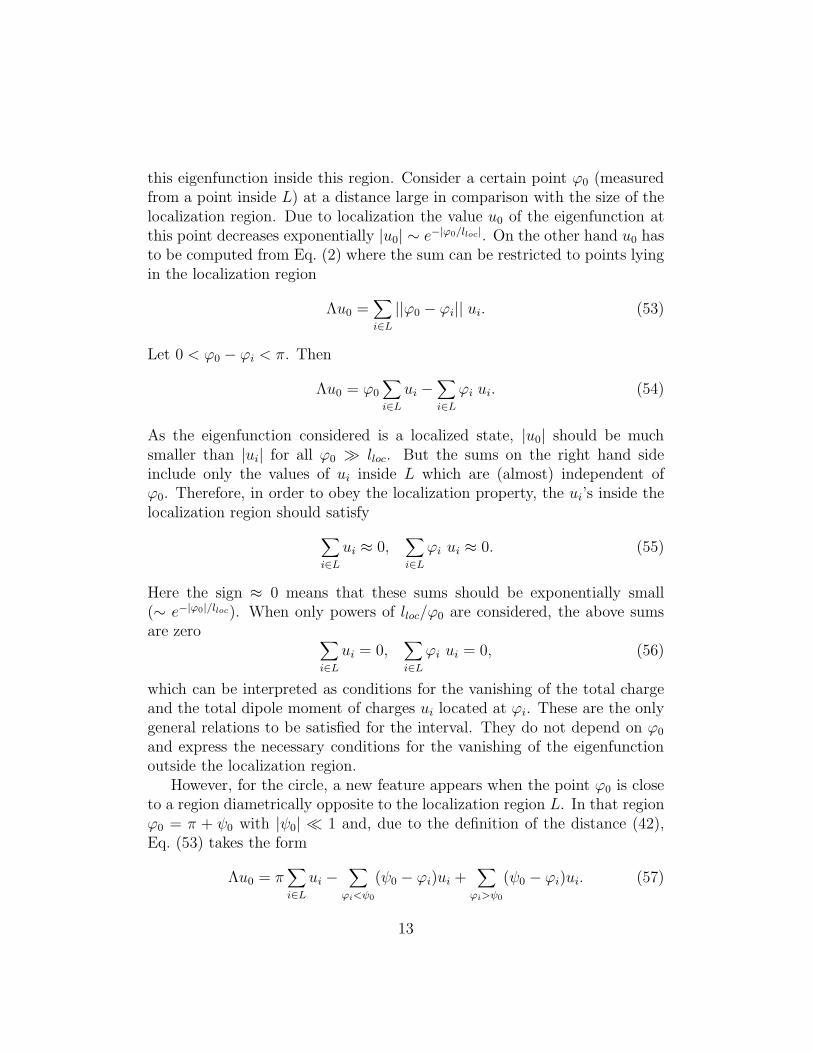
Figure 4: Averaged staircase function with N = 1000 points on the d-dimensional unit sphere (d = 2, 3, 4, 9) showing quasi-degenerate multiplets.For clarity, the counting function has been normalized to N .

From properties of the Gegenbauer polynomials (see e.g. [8] V. 2, 10.9) itfollows that all Λl with even l 6= 0 are zero and consequently beyond the reachof the continuous approximation (see Section 4.3). The value correspondingto l = 0 is the Perron-Frobenius eigenvalue. We therefore concentrate on oddvalues of l.

In the continuous approximation the eigenvalues for d-dimensional sphe-res are h(2k + 1, d − 1) times degenerate. For the one-dimensional sphere(i.e. the circle) h(2k + 1, 0) = 2 as has been seen in Section 3. For the2-sphere (the usual sphere) h(2k + 1, 1) equals 3, 7, 11 . . ., for the 3-spherethe first multiplicities are 4, 16, 36, . . ., for the 4-sphere they are 5, 30, 91, . . . ,etc. In general the first multiplet for the d-sphere corresponding to l = 1 hasmultiplicity d + 1, i.e. it is equal to the dimension of the embedded space.On Fig. 4 these degeneracies can be read off from the numerically calculatedaverage staircase function for spheres of different dimensions.

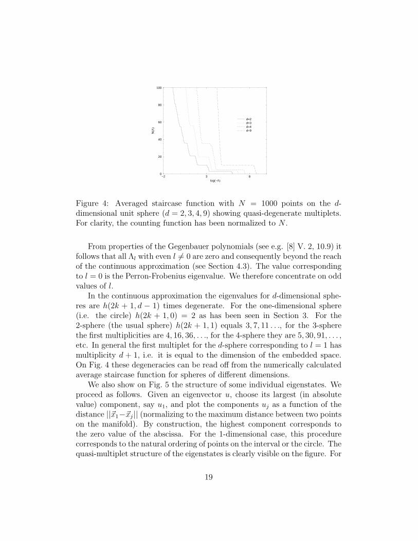
We also show on Fig. 5 the structure of some individual eigenstates. Weproceed as follows. Given an eigenvector u, choose its largest (in absolutevalue) component, say u1, and plot the components uj as a function of thedistance ||~x1−~xj || (normalizing to the maximum distance between two pointson the manifold). By construction, the highest component corresponds tothe zero value of the abscissa. For the 1-dimensional case, this procedurecorresponds to the natural ordering of points on the interval or the circle. Thequasi-multiplet structure of the eigenstates is clearly visible on the figure. For

19

0.0 0.5 1.0−0.1

0

0.10.0 0.5 1.0

−0.1

0

0.10.0 0.5 1.0

−0.1

0

0.10.0 0.5 1.0

−0.1

0

0.1

0.0 0.5 1.0

0.0 0.5 1.0

0.0 0.5 1.0

0.0 0.5 1.0

Figure 5: Individual eigenfunctions u(n) corresponding to the n-th eigenvaluewith N = 1000 points on the unit 3-sphere (left hand side) and on the unit2-sphere (right hand side). From top to bottom: n = 1, 5, and 21 for d = 3and n = 1, 4, and 11 for d = 2. These values of n correspond to the lowesteigenvalue of each of the first three quasi-multiplets. The Perron-Frobeniuseigenfunction (n = 1000) is at the bottom. See text for further explanation.

comparison, the Perron-Frobenius eigenstate is also displayed. For spheresits components are constant to within 1/

√N fluctuations.

4.3 Condition for applicability of the continuous ap-

proximation

The continuous approximation is based on the well known fact that underquite general conditions the sum of a large number of independent randomvariables ~xj with distribution dµ(~x) tends to its mean value

1

N

N∑

j=1

f(~xj) =∫

f(~x)dµ(~x) +ζ√N, (72)

where, when N → ∞, ζ is a random variable with zero mean and varianceindependent on N .

This type of ‘ergodic theorem’ makes natural to consider, instead of the

20

true eigenvalue Eq. (2),

Λnu(n)i =

1

N − 1

N∑

j=1

||~xi − ~xj || u(n)j , (73)

its continuous approximation

Λ(c)n un(~x ) =

1

V

∫

X||~x− ~y|| un(~y )d~y (74)

(we introduce for convenience the factor 1/(N − 1) with the correspondingredefinition Λn = Λn/(N − 1) because in the sum in (73) there are onlyN − 1 non-zero terms). Here for simplicity uncorrelated points ~xj uniformlydistributed on the base manifold X (i.e. dµ(~x) = d~x/V ) are considered.

As the kernel of the integral equation (74) is symmetric, its eigenvaluesΛ(c)n are real and its eigenfunctions un(~x ) can be chosen real orthogonal

1

V

∫

Xun(~x )um(~x )d~x = δmn. (75)

Let us first consider the case when the eigenvalue Λ(c)n of the continuous

equation (74) is non degenerate and let us look for solutions of the trueeigenvalue equation (73) in the form

u(n)j = un(~xj) +

∑

m6=n

cmum(~xj), (76)

where cm are considered as small quantities. (This procedure is often usedin perturbation theory when dealing with the Schroedinger equation.) Sub-stituting these expressions in Eq. (73), multiplying both sides by un(~xi), andsumming from i = 1 to N one obtains

Λn1

N

N∑

i=1

un(~xi)

un(~xi) +∑

m6=n

cmum(~xi)

=

1

N(N − 1)

N∑

i,j=1

un(~xi) ||~xi − ~xj ||

un(~xj) +∑

m6=n

cmum(~xj)

. (77)

The mean values of the terms which are multiplied by cm are zero and,consequently, they are of the order of 1/

√N (see Eq. (72)). Therefore in

21

Eq. (77) these terms can be ignored to first order in 1/√N and this equation

is reduced toΛnAN(n) = BN (n), (78)

where

AN (n) =1

N

N∑

i=1

un(~xi)un(~xi), (79)

BN (n) =1

N(N − 1)

N∑

i,j=1

un(~xi) ||~xi − ~xj || un(~xj). (80)

When N → ∞ these sums tend to their mean value plus corrections

AN(n) → 1 +σ(n)√N, BN(n) → Λ(c)

n +Σ(n)√N. (81)

The mean value of σ(n) and Σ(n) is zero. When N → ∞ their variances areindependent on N and can be computed from straightforward calculations.

By taking the average of AN (n) and BN (n) one recovers the continuousapproximation result. The first correction δΛn = Λn − Λ(c)

n is determined bytheir fluctuating part

δΛn =1√N

(Σ(n) − Λ(c)n σ(n)). (82)

The mean value of δΛn is, of course, zero and its variance is equal to

< δΛ2n >=

Λ(c) 2n

Nv2(n), (83)

wherev2(n) =

∫

Xu4n(~x )dµ(~x) − 1, (84)

provided that the un(~x ) are orthogonal. For semiclassical-type solutions(59), where real orthogonal solutions can be chosen in the form

√2 sin ~q~z

and√

2 cos ~q~z, v2(n) = 5, independent of n.If the eigenvalue Λ(c)

n of the continuous equation (74) is h-fold degenerate,a simple extension of the previous arguments leads to an estimate of thesplitting of the degeneracy by including the next order corrections.

22

Let u(m)n (~x ) m = 1, . . . , h be the solutions of the the continuous equation

(74) corresponding to an h-fold degenerate eigenvalue Λ(c)n normalized as

follows ∫

Xu(m)n (~x )u(m′)

n (~x )dµ(~x) = δmm′ . (85)

The total splitting ∆Λn =∑hj=1 δΛ

(j)n is a random variable which has the

following estimate∆Λn

Λ(c)n

= h · ζ · v(n)√N

(86)

with < ζ >= 0 and < ζ2 >= 1 and

v2(n) =1

h2

h∑

m=1

h∑

m′=1

∫

X

[

u(m)n (~x )u(m′)

n (~x )]2dµ(~x) − 1. (87)

More generally, if a function f(Λn) is computed in the continuous approxi-mation, it will have a random (depending on realizations) fluctuation δf(Λn)which to first order in 1/

√N is

δf(Λn) =df(Λn)

dΛn

hΛnζv(n)√N. (88)

We are interested mainly in the counting function. According to Eq. (66) ithas a power-law asymptotics when smoothed over a small window δΛ anddN(Λ)/Λ = νN(Λ)/Λ with ν = −(d+ 1)/d. Consequently

δN(Λ) ∼ N(Λ)ζ√N. (89)

The condition that perturbed eigenvalues do not deviate from the ones com-puted in the continuous approximation (or equivalently that the splitting(83) is much smaller than the distance between multiplets in the continuousapproximation) leads to the following inequality

δN(Λ) ≪ 1

N. (90)

Together with (89) it implies that, in general, the continuous approximationgives correctly the eigenvalues of only the first

√N eigenstates ordered by

increasing eigenvalues and that by increasing N more and more distinct andisolated multiplets are present. In terms of scaled eigenvalues, one has that

23

the continuous approximation can be used for the approximation of non-averaged eigenvalues satisfying

|λ| ≥ N (d+1)/2d. (91)

For smaller |λ| the spacing between successive eigenvalues computed in thecontinuous approximation becomes comparable to the fluctuating correctionsand the mixing of different states is important.

Nevertheless, one can still use the continuous approximation for the cal-culation of average quantities (e.g. the counting function). The main pointis that the first correction to (89) vanishes because the mean value of ζ iszero to first order in 1/

√N . If there are no singularities (which is probably

true for d > 2), the next order correction will be of the order of G(λ)/Nwith a certain function G(λ) and the conditions (90) on the average will bevalid till λ is of the order of 1. Therefore for averaged quantities one canuse the continuous approximation for a finite fraction of the total number ofeigenvalues.

4.4 Strongly localized states

The properties of strongly localized states can be estimated by slightly mod-ifying the arguments used for the one-dimensional case.

For manifolds of the second kind (like for the circle), assume that aneigenfunction is localized in a small region L and ui are (large) values of thiseigenfunction inside this region. Choose the origin somewhere inside thisregion and consider a point ~x0 at large distance from it. The value u0 of theeigenfunction at this point from Eq. (2) is

Λu0 =∑

i∈L

||~x0 − ~xi|| ui. (92)

As ||~x0|| ≫ ||~xi||, the right-hand side of this expression can be expanded intopowers of ~xi

Λu0 = R∑

i∈L

ui +∑

i∈L

~ζ · ~xi ui + . . . , (93)

where R = ||x0|| and ~ζ = ∂||~x0||/∂~x0.As |u0| should decrease exponentially with R and each term in the above

equation decreases as a different power of R, one concludes, similar to the

24

case of the circle, that in order to obey the localization property ui shouldobey the relations

∑

i∈L

ui ≈ 0,∑

i∈L

~ζ · ~xi ui ≈ 0, etc. (94)

In regions not too close to a region diametrically opposite to the localizationregion ~ζ = ~x0/R and these equations take the form of zero multipole moments

∑

i∈L

ui = 0,∑

i∈L

~xiui, . . . (95)

But close to the diametrically opposite region there are points for which thedistance changes its form as in Eq. (42). For these points the derivative of ||~x||will change sign and, in general, conditions (95) will be impossible to fulfill.Consequently, the eigenfunction in the diametrically opposite region cannot,in general, be exponentially small as required by the usual localization theory.

The above discussion about the localization ‘echo’ is valid for manifoldsof the second kind (i.e. if there exist a few geodesics connecting two points)e.g. for spheres of different dimensions. In Fig. 6 we present the structure ofthe localized eigenfunctions of the distance matrices for 2 and 3 dimensionalspheres in the same way as it was done in Fig. 5. In all cases the eigen-functions have large values near the left and right ends of the interval, inagreement with localization on two diametrically opposite regions. Compari-son with Fig. 5 illustrates also the completely different structure of extendedand localized states (notice the difference in scale in both figures).

To compute the density of strongly localized states let us, as above, as-sume that an eigenfunction is localized in a small region L and denote by uiits large components inside L. (For simplicity we consider only manifolds ofthe first kind.)

The eigenvalue equation (2) gives

Λui =∑

j∈L

||~xi − ~xj || uj. (96)

Because we assume that all ui are localized (are large) in a small region, alldifferences ||~xi−~xj || are of the order of the distance r between nearest points

Λui ≈ r∑

j 6=i

uj. (97)

25

0.0 0.5 1.0−0.7

0

0.70.0 0.5 1.0

−0.7

0

0.70.0 0.5 1.0

−0.7

0

0.70.0 0.5 1.0

−0.7

0

0.7

0.0 0.5 1.0

0.0 0.5 1.0

0.0 0.5 1.0

0.0 0.5 1.0

Figure 6: Individual eigenfunctions u(n) as for Fig. 5 except n = 800, 801,802, 803 for d = 3 and n = 650, 651, 652, 653 for d = 2 from top to bottom.All states are localized.

26

As already indicated in Eq. (94), one of the necessary conditions of localiza-tion is

ui +∑

j 6=i

uj = 0. (98)

ThereforeΛ ≈ −r, (99)

which means that the distribution of eigenvalues of localized states is approx-imately the same as the distribution of distances between two uncorrelatedpoints randomly distributed on the manifold. For small distances the latteris proportional to the volume and, consequently, the staircase function atsmall negative λ is

N(λ) ≈ 1 −Kd(−λ)d, (100)

where Kd is a constant depending on the dimensionality of the system. (Insituations where points though uniformly distributed exhibit repulsion weexpect that the exponent in Eq. (100) will be larger.)

On Fig. 7 (same numerical data as for Fig. 3) the small Λ behaviour ofthe staircase function is displayed. It is clear that the estimate (100) is ingood agreement with the numerical simulations.

Eq.(100) together with Eq. (66), which govern the small and large λbehaviour of the average staircase function respectively, strongly suggest thatN(λ) is independent on the number of points N when N → ∞. This isillustrated on Fig. 8 .

To get further insight on localization properties let us first remind somequalitative properties of the Anderson model. In one dimension all statesare localized, irrespective of the size of disorder. In two dimensions pertur-bation theory cannot be applied and the localization length increases ex-ponentially when disorder decreases. For dimensions larger than two thereis a localization-delocalization transition at finite strength of disorder andthe threshold value increases with dimensionality of the system. For dis-tance matrices, the parameter governing the size of the disorder is the scaledeigenvalue λ = Λ(N/V )1/d, with increasing disorder as |λ| → 0. In Fig. 9 wepresent the numerically computed participation ratio for spheres of dimen-sions 2 and 3. For the 3-sphere the effect of the localization-delocalizationtransition (i.e. the sharp increase of the localization length at a finite valueof λ) is clearly visible.

27

−20 −10 0log(−Λ)

−10

−5

0

log(

1−N

(Λ))

Figure 7: Averaged fraction of eigenvalues above Λ with N = 1000 points inthe unit hyper-cube of dimension d = 1, 2, 3, 4, 5 (from left to right). Straightlines of slope d as predicted by Eq. (100), for comparison.

−2 0 2 4 6log(−λ)

−6

−4

−2

0

log(

N(λ

))

N=100N=200N=500N=1000

Figure 8: Averaged staircase function for the unit 3-dimensional cube fordifferent number of points.

28

−2 0 2 4 6 8log(−λ)

0

2

4

6

8lo

g(R

)

N=5000N=1000N=500N=250N=100

−2 0 2 4 6 8log(−λ)

0

2

4

6

8

log(

R)

N=5000N=1000N=500N=250N=100

Figure 9: Participation ratio corresponding to a single realization for 2-dimensional (left part) and 3-dimensional (right part) unit sphere smoothedover a small window δλ with different number N of points . The abscissaaxis is log(−λ) where λ = ΛN1/2 (left part) and λ = ΛN1/3 (right part).

5 Summary and conclusions

Let N points be distributed on a certain manifold. The (i, j) matrix elementof the distance matrix is defined as the distance between points i and j.Schoenberg [3] proved long time ago that for Euclidean manifolds all eigen-values of such matrices, except one, are non-positive. This property can beextended to other manifolds, in particular, for spherical manifolds treatedhere (see [4] for a general discussion).

The study of the one-dimensional case (interval and circle) provides al-ready some clues of what are the ingredients governing the properties inhigher dimensions and the properties related to the very simple crystal con-figuration are partially kept when ‘disorder’ is added.

In general it is demonstrated that, if the points are uncorrelated anduniformly distributed on a base manifold, the average density of eigenvaluesof distance matrices in the limit N → ∞ has a power-law behaviour forlarge and small negative eigenvalues, the exponent depending only on thedimension of the manifold (see Eqs. (66) and (100)).

The eigenfunctions of the distance matrices with large negative eigenval-ues are delocalized (for 1 and 2 dimensional manifolds the localization lengthis much larger than the system size) whereas the eigenfunctions with very

29

small negative eigenvalues are strongly localized.If the manifold possess a symmetry group, large negative eigenvalues form

almost degenerate multiplets whose dimensions equal the dimensions of theirreducible representations of the group and the conditions for the presenceof isolated multiplets are established.

A distinction among base manifolds for which two points are connectedby one or several geodesics is made. In the latter case the eigenfunctions ofthe distance matrix are, in general, localized not in one but in several regions(echo). For spheres of any dimension we find strongly localized states in twodiametrically opposite regions. The understanding of the structure of theecho for more general spaces deserves further study.

Strongly localized states are, by definition, mostly sensitive to local prop-erties of the base manifold. The existence of the echo shows, however, thatcertain global properties of the manifold are reflected on these states as well.

What precedes is illustrated in detail by studying distance matrices ofuncorrelated points uniformly distributed on hyper-spheres and hyper-cubesof different dimensions.

The introduction of distance matrices in Ref. [1] was to a large extentmotivated by the fact that they encode the metric properties of the basemanifold. Our results show one possible way of solving the inverse problem,namely, the reconstruction of the initial manifold from the knowledge of thespectral properties of its distance matrix. We demonstrate that large negativeeigenvalues can be approximated with 1/

√N accuracy by the solutions of the

continuous approximation Eq. (58). As this integral equation is similar tothe Laplace equation, one may conjecture that for this equation, similarlyas for the former, the question raised by Kac “Can one hear the shape ofa drum?”[9] can also be answered affirmatively, except probably for veryspecial isospectral cases.

When completing this work we became aware of Ref. [10] where EuclideanRandom Matrices were introduced. Matrix elements are then a function offinite range of the relative distance between two points in Euclidean spaceMij = f(||~xi− ~xj ||). One of the main differences with respect to the presentwork is that in [10] the results strongly depend on the choice of f whereashere it is kept fixed f(x) = x and emphasis is put on the choice of themanifold.

Acknowledgments

30

The authors are greatly indebted to A.M. Vershik for discussing his work[1] prior the publication and to M. Mezard for pointing out reference [10].One of the authors (O.B.) acknowledges hospitality at the MFI Oberwolfach,where this work originated.

References

[1] A.M. Vershik, Distance matrices, random metrics and Urysohn space.Preprint MPIM Bonn (2002), math.GT/0203008.

[2] F.R. Gantmacher, Theorie des Matrices, V. 1 and 2, Dunod, Paris(1966).

[3] I.J. Schoenberg, On certain metric spaces arising from euclidean spacesby a change of metric and their imbedding in Hilbert space, Ann. Math.

38 724-732 (1937).

[4] E. Bogomolny, O. Bohigas, and C. Schmit, Distance matrices and iso-metric embedding, (2002) to be published.

[5] I.M. Lifshits, S.A. Gradeskul, and L. Pastur, Introduction to the theory

of disordered systems, John Wiley and Sons, New York (1987).

[6] B. Derrida and E. Gardner, Lyapunov exponent of the one-dimensionalAnderson model: weak disorder expansions, J. Physique 45 1283-1295(1984).

[7] M.L. Mehta, Matrix Theory, Selected Topics and Useful Results, LesEditions de Physique, Les Ulis (1989).

[8] Higher transcendental functions, A. Erdelyi Ed., McGraw-Hill, NewYork, Toronto, London (1953).

[9] M. Kac, Can one hear the shape of a drum? Am. Math. Monthly 73,1-23 (1966).

[10] M. Mezard, G. Parisi, and A. Zee, Spectra of Euclidean Random Matri-ces, Nucl. Phys. B 559, 689-701 (1999).

31