Approximating the Spectral Sums of Large-scaleMatrices using Chebyshev Approximations∗

Insu Han † Dmitry Malioutov ‡ Haim Avron § Jinwoo Shin ¶

June 20, 2018

Abstract

Computation of the trace of a matrix function plays an important role in many scientific com-puting applications, including applications in machine learning, computational physics (e.g., lat-tice quantum chromodynamics), network analysis and computational biology (e.g., protein fold-ing), just to name a few application areas. We propose a linear-time randomized algorithm forapproximating the trace of matrix functions of large symmetric matrices. Our algorithm is basedon coupling function approximation using Chebyshev interpolation with stochastic trace estima-tors (Hutchinon’s method), and as such requires only implicit access to the matrix, in the formof a function that maps a vector to the product of the matrix and the vector. We provide rigorousapproximation error in terms of the extremal eigenvalue of the input matrix, and the Bernsteinellipse that corresponds to the function at hand. Based on our general scheme, we provide algo-rithms with provable guarantees for important matrix computations, including log-determinant,trace of matrix inverse, Estrada index, Schatten p-norm, and testing positive definiteness. Weexperimentally evaluate our algorithm and demonstrate its effectiveness on matrices with tens ofmillions dimensions.

1 Introduction

Given a symmetric matrix A ∈ Rd×d and function f : R→ R, we study how to efficiently compute

Σf (A) = tr(f(A)) =

d∑i=1

f(λi), (1)

where λ1, . . . , λd are eigenvalues of A. We refer to such sums as spectral sums. Spectral sumsdepend only on the eigenvalues of A and so they are spectral functions, although not every spectralfunction is a spectral sum. Nevertheless, the class of spectral sums is rich and includes useful∗This article is partially based on preliminary results published in the proceeding of the 32nd International Conference on

Machine Learning (ICML 2015).†School of Electrical Engineering, Korea Advanced Institute of Science and Technology, Korea. Emails:

hawki17@kaist.ac.kr‡Business Analytics and Mathematical Sciences, IBM Research, Yorktown Heights, NY, USA. Email:

dmalioutov@us.ibm.com§Department of Applied Mathematics, Tel Aviv University. Email: haimav@post.tau.ac.il¶School of Electrical Engineering, Korea Advanced Institute of Science and Technology, Korea. Email: jin-

woos@kaist.ac.kr

1

arX

iv:1

606.

0094

2v1

[cs

.DS]

3 J

un 2

016

spectral functions. For example, if A is also positive definite then Σlog(A) = log det(A), i.e. thelog-determinant of A.

Indeed, there are many real-world applications in which spectral sums play an important role. Forexample, the log-determinant appears ubiquitously in machine learning applications including Gaus-sian graphical and Gaussian process models [40, 38, 15], partition functions of discrete graphicalmodels [31], minimum-volume ellipsoids [46], metric learning and kernel learning [12]. The traceof the matrix inverse (Σf (A) for f(x) = 1/x) is frequently computed for the covariance matrixin uncertainty quantification [11, 29] and lattice quantum chromodynamics [41]. The Estrada in-dex (Σexp(A)) has been initially developed for topological index of protein folding in the studyof protein functions and protein-ligand interactions [17, 14], and currently it appears in numerousother applications, e.g., statistical thermodynamics [20, 19], information theory [9] and networktheory [21, 18] ; see Gutman et al. [24] for more applications. The Schatten p-norm (Σf (A)2/p

for f(x) = xp/2 for p ≥ 1 ) has been applied to recover low-rank matrix [36] and sparse MRIreconstruction [32].

The computation of the aforementioned spectral sums for large-scale matrices is a challenging task.For example, the standard method for computing the log-determinant uses the Cholesky decompo-sition (if A = LLT is a Cholesky decomposition, then log det(A) = 2

∑i logLii). In general,

the computational complexity of Cholesky decomposition is cubic with respect to the number ofvariables, i.e. O(d3). For large-scale applications involving more than tens of thousands of dimen-sions, this is obviously not feasible. If the matrix is sparse, one might try to take advantage ofsparse decompositions. As long as the amount of fill-in during the factorizations is not too big, asubstantial improvement in running time can be expected. Nevertheless, the worst case still requiresΘ(d3). In particular, if the sparsity structure of A is random-like, as is common in several of theaforementioned applications, then little improvement can be expected with sparse methods.

Our aim is to design an efficient algorithm that is able to compute accurate approximations to spectralsums for matrices with tens of millions of variables.

1.1 Contributions

We propose a randomized algorithm for approximating spectral sums based on a combination ofstochastic trace-estimators and Chebyshev interpolation. Our algorithm first computes the coeffi-cients of a Chebyshev approximation of f . This immediately leads to an approximation of the spec-tral sum as the trace of power series of the input matrix. We then use a stochastic trace-estimator toestimate this trace. In particular, we use Hutchinson’s method [27].

One appealing aspect of Hutchinson’s method is that it does not require an explicit representationof the input matrix; Hutchinson’s method requires only an implicit representation of the matrix asan operation that maps a vector to the product of the matrix with the vector. In fact, this property isinherited by our algorithm to its entirety: our algorithm only needs access to an implicit represen-tation of the matrix as an operation that maps a vector to the product of the matrix with the vector.In accordance, we measure the complexity of our algorithm in terms of the number of matrix-vectorproducts that it requires. We establish rigorous bounds on the number of matrix-vector products forattaining a ε-multiplicative approximation of the spectral sum based on ε, the failure probability andthe range of the function over its Bernstein ellipse (see Theorem 5 for details). In particular, Theo-rem 5 implies that if the range is Θ(1), then the algorithm provides ε-multiplicative approximation

2

guarantee using a constant amount of matrix-vector products for any constant ε > 0 and constantfailure probability.

The overall time complexity of our algorithm is O(t · ‖A‖mv) where t is the number of matrix-vector products (as established by our analysis) and ‖A‖mv is the cost of multiplying A by a vector.One overall assumption is that matrix-vector products can be computed efficiently, i.e. ‖A‖mv issmall. For example, if A is sparse then ‖A‖mv = O(nnz(A)), i.e., the number of non-zero entriesin A. Other cases that admit fast matrix-vector products are low-rank matrices (which allow fastmultiplication by factorization), or Fourier (or Hadamard, Walsh, Toeplitz) matrices using the fastFourier transform. The proposed algorithm is also very easy to parallelize.

We then proceed to discuss applications of the proposed algorithm. We give rigorous bounds forusing our algorithm for approximating the log-determinant, trace of the inverse of a matrix, theEstrada index, and the Schatten p-norm. These correspond to continuous functions f(x) = log x,f(x) = 1/x, f(x) = exp(x) and f(x) = xp/2, respectively. We also use our algorithm to constructa novel algorithm for testing positive definiteness in the property testing framework. Our algorithm,which is based on approximating the spectral sum for 1−sign(x), is able to test positive definitenessof a matrix with a sublinear (in matrix size) number of matrix-vector products.

Our experiments show that our proposed algorithm is orders of magnitude faster than the standardmethods for sparse matrices and provides approximations with less than 1% error for the exampleswe consider. It can also solve problems of tens of millions dimension in a few minutes on our singlecommodity computer with 32 GB memory. Furthermore, as reported in our experimental results,it achieves much better accuracy compared to a similar approach based on Talyor expansions [50],while both have similar running times. In addition, it outperforms the recent method based onCauchy integral formula [2] in both running time and accuracy.1 The proposed algorithm is alsovery easy to parallelize and hence has a potential to handle even larger problems. For example, theSchur method was used as a part of QUIC algorithm for sparse inverse covariance estimation withover million variables [26], hence our log-determinant algorithm could be used to further improveits speed and scale.

1.2 Related Work

Bai et al. [5] were the first to consider the problem of approximating spectral sums, and its specificuse for approximating the log-determinant and the trace of the matrix inverse. Like our method,their method combines stochastic trace estimation with approximation of bilinear forms. However,their method for approximating bilinear forms is fundamentally different than our method and isbased on a Gauss-type quadrature of a Riemann-Stieltjes integral. They do not provide rigorousbounds for the bilinear form approximation. In addition, recent progress on analyzing stochastictrace estimation [4, 39] allow us to provide rigorous bounds for the entire procedure.

Since then, several authors considered the use of stochastic trace estimators to compute certain spec-tral sums. Bekas et al. [6] and Malioutov et al. [33] consider the problem of computing the diagonalof a matrix or of the matrix inverse. Saad et al. [16] use polynomial approximations and rationalapproximations of high-pass filter to count the number of eigenvalues in an input interval. They donot provide rigorous bounds. Stein et al. [42] use stochastic approximations of score functions tolearn large-scale Gaussian processes.

1Aune et al.’s method [2] is implemented in the SHOGUN machine learning toolbox, http://www.shogun-toolbox.org.

3

Approximation of the log-determinant in particular has received considerable treatment in the lit-erature. Pace and LeSage [37] use both Taylor and Chebyshev based approximation to the loga-rithm function to design an algorithm for log-determinant approximation, but do not use stochastictrace estimation. Their method is determistic, can entertain only low-degree approximations, andhas no rigorous bounds. Zhang and Leithead [50] consider the problem of approximating the log-determinant in the setting of Gaussian process parameter learning. They use Taylor expansion inconjunction with stochastic trace estimators, and propose novel error compensation methods. Theydo not provide rigorous bounds as we provide for our method. Boutsidis et al. [8] use a similarscheme based on Taylor expansion for approximating the log-determinant, and do provide rigorousbounds. Nevertheless, our experiments demonstrate that our Chebyshev interpolation based methodprovides superior accuracy. Aune et al. [2] approximate the log-determinant using a Cauchy integralformula. Their method requires the multiple use of a Krylov-subspace linear system solver, so theirmethod is rather expensive. Furthermore, no rigorous bounds are provided.

Computation of the trace of the matrix inverse has also been researched extensively. One recentexample is the work of Wu et al. [48] use a combination of stochastic trace estimation and inter-polating an approximate inverse. In another example, Chen [10] considers how accurately shouldlinear systems be solved when stochastic trace estimators are used to approximate the trace of theinverse.

To summarize, the main novelty of our work is combining Chebyshev interpolation with Hutchin-son’s trace estimator, which allows to design an highly effective linear-time algorithm with rigorousapproximation guarantees for general spectral sums.

1.3 Organization

The structure of the paper is as follows. We introduce the necessary background in Section 2. Section3 provides the description of our algorithm with approximation guarantees, and its applications tothe log-determinant, the trace of matrix inverse, the Estrada index, the Schatten p-norm and testingpositive definiteness are described in Section 4. We report experimental results in Section 5.

2 Preliminaries

Throughout the paper, A ∈ Rd×d is a symmetric matrix with eigenvalues λ1, . . . , λd ∈ R and Idis the d-dimensional identity matrix. We use tr(·) to denote the trace of the matrix. We also useλmin(A) and λmax(A) to denote the smallest and largest eigenvalue of A. In particular, we assumethat an interval [a, b] in which contains all of A’s eigenvalues is given. In some cases, such boundsare known a-priori due to properties of the downstream use (e.g., the application considered inSection 5.3). In others, a crude bound like a = −‖A‖∞ and b = ‖A‖∞ or via Gershgorin’s CircleTheorem [23, Section 7.2] might be obtained. For some functions, our algorithm has additionalrequirements on a and b (e.g. for log-determinant, we need a > 0).

Our approach combines two techniques, which we discuss in detail in the next two subsections:(a) designing polynomial expansion for given function via Chebyshev interpolation [34] and (b)approximating the trace of matrix via Monte Carlo methods [27].

4

2.1 Function Approximation using Chebyshev Interpolation

Chebyshev interpolation approximates an analytic function by interpolating the function at theChebyshev nodes using a polynomial. Conveniently, the interpolation can be expressed in termsof basis of Chebyshev polynomials. Specifically, the Chebyshev interpolation pn of degree n for agiven function f : [−1, 1]→ R is given by (see Mason and Handscomb [34]):

f(x) ≈ pn(x) =

n∑j=0

cjTj(x) (2)

where the coefficient cj , the j-th Chebyshev polynomial Tj(x) and Chebyshev nodes {xk}nk=0 aredefined as

cj =

1

n+ 1

n∑k=0

f(xk) T0(xk) if j = 0

2

n+ 1

n∑k=0

f(xk) Tj(xk) otherwise

(3)

T0(x) = 1, T1(x) = x

Tj+1(x) = 2xTj(x)− Tj−1(x) for j ≥ 1 (4)

xk = cos(π(k + 1/2)

n+ 1

).

Chebyshev interpolation better approximates the functions as the degree n increases. In particular,the following error bound is known [7, 49].

Theorem 1 Suppose f is analytic function with |f(z)| ≤ U in the region bounded by the so-calledBernstein ellipse with foci +1,−1 and sum of major and minor semi-axis lengths equals to ρ > 1.Let pn denote the degree n Chebyshev interpolant of f as defined by equations (2), (3) and (4). Wehave,

maxx∈[−1,1]

|f(x)− pn(x)| ≤ 4U

(ρ− 1) ρn.

The interpolation scheme described so far assumed a domain of [−1, 1]. To allow a more generaldomain of [a, b] one can use the linear mapping g(x) = b−a

2 x+ b+a2 to map [−1, 1] to [a, b]. Thus,

f ◦g is a function on [−1, 1] which can be approximated using the scheme above. The approximationto f is then pn = pn ◦ g−1 where pn is the approximation to f ◦ g. Note that pn is a polynomialwith degree n as well. In particular, we have the following approximation scheme for a generalf : [a, b]→ R:

f(x) ≈ pn(x) =

n∑j=0

cjTj

(2

b− ax− b+ a

b− a

)(5)

5

where the coefficient cj are defined as

cj =

1

n+ 1

n∑k=0

f

(b− a

2xk +

b+ a

2

)T0(xk) if j = 0

2

n+ 1

n∑k=0

f

(b− a

2xk +

b+ a

2

)Tj(xk) otherwise

(6)

The following is simple corollary of Theorem 1.

Corollary 2 Suppose that a, b ∈ R with a < b. Suppose f is analytic function with∣∣f( b−a2 z + b+a

2 )∣∣ ≤

U in the region bounded by the ellipse with foci +1,−1 and sum of major and minor semi-axislengths equals to ρ > 1. Let pn denote the degree n Chebyshev interpolant of f on [a, b] as definedby equations (5), (6) and (4). We have,

maxx∈[a,b]

|f(x)− pn(x)| ≤ 4U

(ρ− 1) ρn.

Proof. Follows immediately from Theorem 1 and observing that for g(x) = b−a2 x+ b+a

2 we have

maxx∈[−1,1]

|(f ◦ g)(x)− pn (x)| = maxx∈[a,b]

|f(x)− pn (x)| .

Chebyshev interpolation for scalar functions can be naturally generalized to matrix functions [25].Using the Chebyshev interpolation pn for function f , we obtain the following approximation for-mula:

Σf (A) =

d∑i=1

f(λi) ≈d∑i=1

pn(λi) =

d∑i=1

n∑j=0

cjTj

(2

b− aλi −

b+ a

b− a

)

=

n∑j=0

cj

d∑i=1

Tj

(2

b− aλi −

b+ a

b− a

)=

n∑j=0

cjtr

(Tj

(2

b− aA− b+ a

b− aId

))

= tr

n∑j=0

cjTj

(2

b− aA− b+ a

b− aId

)where the equality before the last follows from the fact that

∑di=1 p(λi) = tr(p(A)) for any poly-

nomial p, and the last equality from the linearity of the trace operation.

We remark that other polynomial approximations, e.g. Taylor, can also be used. However, it knownthat Chebyshev interpolation, in addition to its simplicity, is nearly optimal [45] with respect to the∞-norm so is well-suited for our uses.

2.2 Stochastic Trace Estimation (Hutchinson’s Method)

The main challenge in utilizing the approximation formula at the end of the last subsection is howto compute

tr

n∑j=0

cjTj

(2

b− aA− b+ a

b− aId

)6

without actually computing the matrix involved (since the latter is expensive to compute). In thispaper we turn to the stochastic trace estimation method. In essence, it is a Monte-Carlo approach:to estimate the trace of an arbitrary matrix B, first a random vector z is drawn from some fixeddistribution, such that the expectation of z>Bz is equal to the trace of B. By sampling m suchi.i.d. random vectors, and averaging we obtain an estimate of tr(B). Namely, given random vectorsv(1), . . . ,v(m), the estimator is

trm(B) =1

m

m∑i=1

v(i)>Bv(i) .

It is known that trace estimator using i.i.d. random vectors whose entries are chosen uniformly from{−1,+1} has the smallest variance among such Monte-Carlo methods [27, 4]. This estimator isknown as the Hutchinson’s estimator, and has found use in many applications [3, 27, 1]. Formally,this trace estimator trm(B) is known to satisfy the following equalities:

E [trm (B)] = tr (B)

Var [trm (B)] =2

m

(‖B‖2F −

d∑i=1

B2i,i

)However, (ε, ζ)-bounds, as introduced by Avron et al. [4], are more appropriate for our needs.Specifically, we use the following bound due to Roosta-Khorasani and Ascher [39].

Theorem 3 Let B ∈ Rd×d be a positive (or negative) semi-definite matrix. Given ε, ζ ∈ (0, 1),

Pr [|trm(B)− tr(B)| ≤ ε |tr(B)|] ≥ 1− ζ

holds if sampling number m is larger than 6ε−2 log(

2ζ

).

Note that computing v(i)>Bv(i) requires only multiplications between a matrix and a vector, whichis particularly appealing when evaluating B itself is expensive, e.g.,

B =

n∑j=0

cjTj

(2

b− aA− b+ a

b− aId

)as in our case. In this case,

v(i)>Bv(i) =

n∑j=0

cjv(i)>Tj

(2

b− aA− b+ a

b− aId

)v(i) =

n∑j=0

cjv(i)>w

(i)j

where

w(i)j = Tj

(2

b− aA− b+ a

b− aId

)v(i) .

The latter can be computed efficiently (using n matrix-vector products with A) by observing thatdue to equation (4) we have that

w(i)0 = v(i),w

(i)1 =

(2

b− aA− b+ a

b− aId

)w

(i)0

w(i)j+1 = 2

(2

b− aA− b+ a

b− aId

)w

(i)j −w

(i)j−1 .

7

In order to apply Theorem 3 we need B to be positive (or negative) semi-definite. In our caseB = pn(A) so it is sufficient for pn to be non-negative (non-positive). The following lemmaestablishes a sufficient condition for non-negativity of pn, and a consequence positive (negative)semi-definiteness of pn(A).

Lemma 4 Suppose f satisfies that |f(x)| ≥ L for x ∈ [a, b] Then, linear transformed Chebyshevapproximation pn(x) of f(x) is also positive-valued in [a, b] if

4U

(ρ− 1) ρn≤ L (7)

holds for all n ≥ 1.

Proof. From Corollary 2, we have

min[a,b]

pn(x) = min[a,b]

f(x) + (pn(x)− f(x))

≥ min[a,b]

f(x)−max[a,b]|pn(x)− f(x)|

≥ L− 4U

(ρ− 1) ρn≥ 0.

where the last inequality uses Corollary 2. This completes the proof of Lemma 4.

3 Approximating Spectral Sums

3.1 Algorithm Description

Our algorithm brings together the components discussed in the previous section. A pseudo-codedescription appears as Algorithm 1. As mentioned before, we assume that eigenvalues of A are inthe interval [a, b] for some b > a.

In Section 4, we provide five concrete applications of the above algorithm: approximating the log-determinant, the trace of matrix inverse, the Estrada index, the Schatten p-norm and testing positivedefiniteness, which correspond to log x, 1/x, exp(x), xp/2 and 1− sign(x) respectively.

3.2 Analysis

We establish the following theoretical guarantee on the proposed algorithm.

Theorem 5 Suppose function f satisfies the followings:

• f is non-negative (or non-positive) on [a, b].

• f is analytic with∣∣f ( b−a2 z + b+a

2

)∣∣ ≤ U for some U < ∞ on the elliptic region Eρ in thecomplex plane with foci at −1,+1 and ρ as the sum of semi-major and semi-minor lengths.

• minx∈[a,b] |f(x)| ≥ L for some L > 0.

8

Algorithm 1 Trace of matrix function f approximationInput: symmetric matrix A ∈ Rd×d with eigenvalues in [a, b], sampling number m and polyno-mial degree nInitialize: Γ← 0for j = 0 to n docj ← j-th coefficient of the Chebyshev interpolation of f on [a, b] (see equation (6)).

end forfor i = 1 to m do

Draw a random vector v(i) ∈ {−1,+1}d whose entries are uniformly distributedw

(i)0 ← v(i) and w

(i)1 ← 2

b−aAv(i) − b+a

b−av(i)

u← c0w(i)0 + c1w

(i)1

for j = 2 to n dow

(i)2 ← 4

b−aAw(i)1 −

2(b+a)b−a w

(i)1 −w

(i)0

u← u + cj w2

w(i)0 ← w

(i)1 and w

(i)1 ← w

(i)2

end forΓ← Γ + v(i)>u/m

end forOutput: Γ

Given ε, ζ ∈ (0, 1), if

m ≥ 54ε−2 log (2/ζ),

n ≥ log

(8

ε(ρ− 1)

U

L

)/ log ρ,

thenPr (|Σf (A)− Γ| ≤ ε |Σf (A)|) ≥ 1− ζ.

where Γ is the output of Algorithm 1.

The number of matrix-vector products performed by Algorithm 1 isO(mn), thus the time-complexityis O(mn‖A‖mv), where ‖A‖mv is that of the matrix-vector operation. In particular, if m,n = O(1),the complexity is linear with respect to ‖A‖mv. Therefore, Theorem 5 implies that if U,L = Θ(1),then one can choose m,n = O(1) for ε-multiplicative approximation with probability of at least1− ζ given constants ε, ζ > 0.

Proof. The condition

n ≥ log

(8

ε(ρ− 1)

U

L

)/ log ρ

implies that

4U

(ρ− 1) ρn≤ ε

2L (8)

Recall that the trace of a matrix is equal to the sum of its eigenvalues and this also holds for afunction of the matrix, i.e., f(A). Under this observation, we establish a matrix version of Corollary

9

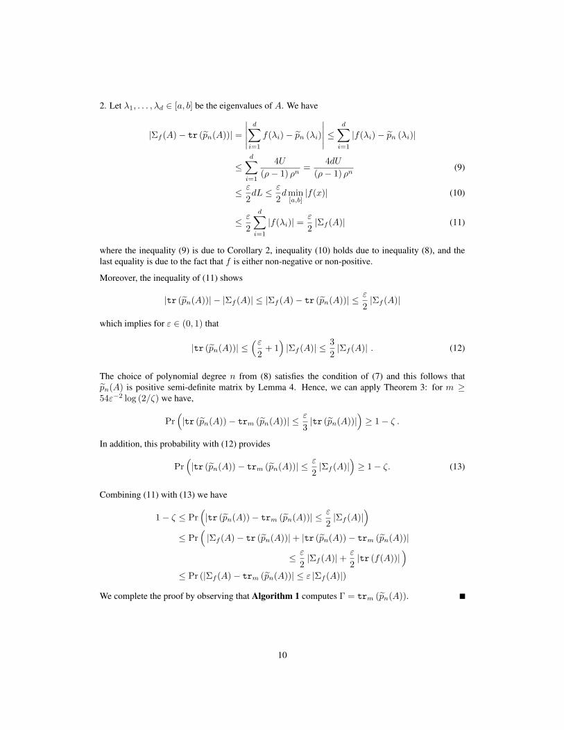
2. Let λ1, . . . , λd ∈ [a, b] be the eigenvalues of A. We have

|Σf (A)− tr (pn(A))| =

∣∣∣∣∣d∑i=1

f(λi)− pn (λi)

∣∣∣∣∣ ≤d∑i=1

|f(λi)− pn (λi)|

≤d∑i=1

4U

(ρ− 1) ρn=

4dU

(ρ− 1) ρn(9)

≤ ε

2dL ≤ ε

2dmin

[a,b]|f(x)| (10)

≤ ε

2

d∑i=1

|f(λi)| =ε

2|Σf (A)| (11)

where the inequality (9) is due to Corollary 2, inequality (10) holds due to inequality (8), and thelast equality is due to the fact that f is either non-negative or non-positive.

Moreover, the inequality of (11) shows

|tr (pn(A))| − |Σf (A)| ≤ |Σf (A)− tr (pn(A))| ≤ ε

2|Σf (A)|

which implies for ε ∈ (0, 1) that

|tr (pn(A))| ≤(ε

2+ 1)|Σf (A)| ≤ 3

2|Σf (A)| . (12)

The choice of polynomial degree n from (8) satisfies the condition of (7) and this follows thatpn(A) is positive semi-definite matrix by Lemma 4. Hence, we can apply Theorem 3: for m ≥54ε−2 log (2/ζ) we have,

Pr(|tr (pn(A))− trm (pn(A))| ≤ ε

3|tr (pn(A))|

)≥ 1− ζ .

In addition, this probability with (12) provides

Pr(|tr (pn(A))− trm (pn(A))| ≤ ε

2|Σf (A)|

)≥ 1− ζ. (13)

Combining (11) with (13) we have

1− ζ ≤ Pr(|tr (pn(A))− trm (pn(A))| ≤ ε

2|Σf (A)|

)≤ Pr

(|Σf (A)− tr (pn(A))|+ |tr (pn(A))− trm (pn(A))|

≤ ε

2|Σf (A)|+ ε

2|tr (f(A))|

)≤ Pr (|Σf (A)− trm (pn(A))| ≤ ε |Σf (A)|)

We complete the proof by observing that Algorithm 1 computes Γ = trm (pn(A)).

10

4 Applications

In this section, we discuss several applications of Algorithm 1: approximating the log-determinant,trace of the matrix inverse, the Estrada index, the Schatten p-norm and testing positive definiteness.Underlying these applications is executing Algorithm 1 with the following functions: f(x) = log x(for log-determinant), f(x) = 1/x (for matrix inverse), f(x) = exp(x) (for the Estrada index),f(x) = xp/2 (for the Schatten p-norm) and f(x) = 1

2 (1 + tanh (−αx)), as a smooth approxima-tion of 1− sign(x) (for testing positive definiteness).

4.1 Log-determinant of Positive Definite Matrices

Since Σlog(A) = log detA our algorithm can naturally be used to approximate the log-determinent.However, it is beneficial to observe that

Σf (A) = Σf (A/(a+ b))− d log(a+ b)

and use Algorithm 1 to approximate Σf (A) for A = A/(a + b). The reason we consider Ainstead of A as an input of Algorithm 1 is because all eigenvalues of A are strictly less than 1 andthe constant L > 0 in Theorem 5 is guaranteed to exist for A. The procedure is summarized in theAlgorithm 2. In the next subsection we generalize the algorithm for general non-singular matrices.

Algorithm 2 Log-deteminant approximation for positive definite matricesInput: positive definite matrix A ∈ Rd×d with eigenvalues in [a, b] for some a, b > 0, samplingnumber m and polynomial degree nInitialize: A← A/ (a+ b)

Γ← Output of Algorithm 1 with inputs A,[

aa+b ,

ba+b

],m, n with f(x) = log x

Γ← Γ + d log (a+ b)

Output: Γ

We note that Algorithm 2 requires us to know a positive lower bound a > 0 for the eigenvalues,which is in general harder to obtain than the upper bound b (e.g. one can choose b = ‖A‖∞). In somespecial cases, the smallest eigenvalue of positive definite matrices are known, e.g., random matrices[44, 43] and diagonal-dominant matrices [22, 35]. Furthermore, it is sometimes explicitly given asa parameter in many machine learning log-determinant applications [47], e.g., A = aId + B forsome positive semi-definite matrix B and this includes the application involving Gaussian MarkovRandom Fields (GMRF) in Section 5.3.

We provide the following theoretical bound on the sampling number m and the polynomial degreen of Algorithm 2.

Theorem 6 Given ε, ζ ∈ (0, 1), consider the following inputs for Algorithm 2:

• A ∈ Rd×d be a positive definite matrix with eigenvalues in [a, b] for a, b > 0

• m ≥ 54ε−2(log(1 + b

a

))2log(

2ζ

)• n ≥

log(

20ε

(√2ba +1−1

)log(1+(b/a)) log(2+2(b/a))

log (1+(a/b))

)log

(√2(b/a)+1+1√2(b/a)+1−1

) = O

(√ba log

(bεa

))

11

Then, it follows that

Pr [ |log detA− Γ| ≤ εd] ≥ 1− ζ

where Γ is the output of Algorithm 2.

Proof. The proof of Theorem 6 is straightforward using Theorem 5 with choice of upper bound U ,lower bound L and constant ρ for the function log x. Denote δ = a

a+b and eigenvalues of A lie inthe interval [δ, 1 − δ]. We choose the ellipse region, denoted by Eρ, in the complex plane with fociat +1,−1 and its semi-major axis length is 1/(1− δ). Then,

ρ =1

1− δ+

√(1

1− δ

)2

− 1 =

√2− δ +

√δ

√2− δ −

√δ> 1

and log(

(1−2δ)x+12

)is analytic on and inside Eρ in the complex plane.

The upper bound U can be obtained as follows:

maxz∈Eρ

∣∣∣∣log

((1− 2δ) z + 1

2

)∣∣∣∣ ≤ maxz∈Eρ

√(log

∣∣∣∣ (1− 2δ) z + 1

2

∣∣∣∣)2

+ π2

=

√(log

∣∣∣∣ δ

2 (1− δ)

∣∣∣∣)2

+ π2 ≤ 5 log

(2

δ

):= U.

where the inequality in the first line holds because |log z| = |log |z|+ i arg (z)| ≤√

(log |z|)2 + π2

for any z ∈ C and equality in the second line holds by the maximum-modulus theorem. We alsohave the lower bound on log x in [δ, 1− δ] as follows:

min[δ,1−δ]

|log x| = log

(1

1− δ

):= L

With these constants, a simple calculation reveals that Theorem 5 implies that Algorithm 1 approx-imates

∣∣log detA∣∣ with ε/ log(1/δ)-mulitipicative approximation.

The additive error bound now follows by using the fact that∣∣log detA

∣∣ ≤ d log (1/δ) .

The bound on polynomial degree n in the above theorem is relatively tight, e.g., n = 27 for δ = 0.1and ε = 0.01. Our bound for m can yield very large numbers for the range of ε and ζ we areinterested in. However, numerical experiments revealed that for the matrices we were interestedin, the bound is not tight and m ≈ 50 was sufficient for the accuracy levels we required in theexperiments.

4.2 Log-determinant of Non-Singular Matrices

One can apply the algorithm in the previous section to approximate the log-determinant of a non-symmetric non-singular matrix C ∈ Rd×d. The idea is simple: run Algorithm 2 on the positivedefinite matrix C>C. The underlying observation is that

log |detC| = 1

2log detC>C . (14)

12

Without loss of generality, we assume that singular values of C are in the interval [σmin, σmax]for some σmin, σmax > 0, i.e., the condition number κ(C) is at most κmax := σmax/σmin. Theproposed algorithm is not sensitive to tight knowledge of σmin or σmax, but some loose lower andupper bounds on them, respectively, suffice. A pseudo-code description appears as Algorithm 3.

Algorithm 3 Log-determinant approximation for non-singular matricesInput: non-singular matrix C ∈ Rd×d with singular values are in the interval [σmin, σmax] forsome σmin, σmax > 0, sampling number m and polynomial degree n

Γ← Output of Algorithm 2 for inputs C>C,[σ2min, σ

2max

],m, n

Γ← Γ/2

Output: Γ

The time-complexity of Algorithm 3 isO(mn‖C‖mv) = O(mn‖C>C‖mv) as well since Algorithm2 requires the computation of a products of matrix C>C and a vector, and that can be accomplishedby first multiplying by C and then by C>. We state the following additive error bound of the abovealgorithm.

Corollary 7 Given ε, ζ ∈ (0, 1), consider the following inputs for Algorithm 3:

• C ∈ Rd×d be a matrix with singular values in [σmin, σmax] for some σmin, σmax > 0

• m ≥M(ε, σmax

σmin, ζ)

and n ≥ N(ε, σmax

σmin

), where

M(ε, κ, ζ) :=14

ε2(log(1 + κ2

))2log

(2

ζ

)

N (ε, κ) :=log(

10ε

(√2κ2 + 1− 1

) log (2+2κ2)log(1+κ−2)

)log(√

2κ2+1+1√2κ2+1−1

) = O(κ log

κ

ε

)Then, it follows that

Pr [ |log (|detC|)− Γ| ≤ εd ] ≥ 1− ζ

where Γ is the output of Algorithm 3.

Proof. Follows immediately from equation (14) and Theorem 6, and observing that all the eigen-values of C>C are inside [σ2

min, σ2max].

We remark that the condition number σmax/σmin decides the complexity of Algorithm 3. As onecan expect, the approximation quality and algorithm complexity become worse as the conditionnumber increases, as polynomial approximation for log near the point 0 is challenging and requireshigher polynomial degrees.

4.3 Trace of Matrix Inverse

In this section, we describe how to estimate the trace of matrix inverse. Since this task amountsto computing Σf (A) for f(x) = 1/x, we propose Algorithm 4 which uses Algorithm 1 as asubroutine.

13

Algorithm 4 Trace of matrix inverseInput: positive definite matrix A ∈ Rd×d with eigenvalues in [a, b] for some a, b > 0, samplingnumber m and polynomial degree nΓ← Output of Algorithm 1 for inputs A, [a, b],m, n with f(x) = 1

x .Output: Γ

We provide the following theoretical bounds on sampling number m and polynomial degree n ofAlgorithm 4.

Theorem 8 Given ε, ζ ∈ (0, 1), consider the following inputs for Algorithm 4:

• A ∈ Rd×d be a positive definite matrix with eigenvalues in [a, b]

• m ≥ 54ε−2 log(

2ζ

)• n ≥ log

(8ε

(√2(ba

)− 1− 1

)ba

)/ log

(2√

2( ba )−1−1+ 1

)= O

(√ba log

(bεa

))Then, it follows that

Pr[ ∣∣tr (A−1)− Γ

∣∣ ≤ ε ∣∣tr (A−1)∣∣] ≥ 1− ζ

where Γ is the output of Algorithm 4.

Proof. In order to apply Theorem 5, we define inverse function with linear transformation f as

f (x) =1

b−a2 x+ b+a

2

for x ∈ [−1, 1].

Avoiding singularities of f , it is analytic on and inside elliptic region in the complex plane passingthrough b

b−a whose foci are +1 and −1. The sum of length of semi-major and semi-minor axes isequal to

ρ =b

b− a+

√b2

(b− a)2 − 1 =

2√2(ba

)− 1− 1

+ 1.

For the maximum absolute value on this region, f has maximum value U = 2/a at − bb−a . The

lower bound is L = 1/b. Putting those together, Theorem 5, implies the bounds stated in thetheorem statement.

4.4 Estrada Index

Given a (undirected) graph G = (V,E), the Estrada index EE (G) is defined as

EE (G) := Σexp(AG) =

d∑i=1

exp(λi),

where AG is the adjacency matrix of G and λ1, . . . , λ|V | are the eigenvalues of AG. It is a wellknown result in spectral graph theory that the eigenvalues ofAG are contained in [−∆G,∆G] where

14

∆G is maximum degree of a vertex in G. Thus, the Estrada index G can be computed using Al-gorithm 1 with the choice of f(x) = exp(x), a = −∆G, and b = ∆G. However, we state ouralgorithm and theoretical bounds in terms of a general interval [a, b] that bounds the eigenvalues ofAG, to allow for an a-priori tighter bounds on the eigenvalues (note, however, that it is well knownthat always λmax ≥

√∆G.

Algorithm 5 Estrada index approximationInput: adjacency matrix AG ∈ Rd×d with eigenvalues in [a, b], sampling number m and polyno-mial degree n{If ∆G is the maximum degree of G, then a = −∆G, b = ∆G can be used as default.}Γ← Output of Algorithm 1 for inputs A, [a, b],m, n with f(x) = exp(x).Output: Γ

We provide the following theoretical bounds on sampling number m and polynomial degree n ofAlgorithm 5.

Theorem 9 Given ε, ζ ∈ (0, 1), consider the following inputs for Algorithm 5:

• AG ∈ Rd×d be an adjacency matrix of a graph with eigenvalues in [a, b].

• m ≥ 54ε−2 log(

2ζ

)• n ≥ log

(2πε (b− a) exp

(√16π2+(b−a)2+(b−a)

2

))/ log

(4πb−a + 1

)= O

(b−a+log 1

ε

log( 1b−a )

)Then, it follows that

Pr [ |EE (G)− Γ| ≤ ε |EE (G)|] ≥ 1− ζ

where Γ is the output of Algorithm 5.

Proof. We consider exponential function with linear transformation as

f (x) = exp

(b− a

2x+

b+ a

2

)for x ∈ [−1, 1].

The function f is analytic on and inside elliptic region in the complex plane which has foci ±1 andpasses through 4πi

(b−a) . The sum of length of semi-major and semi-minor axes becomes

4π

b− a+

√16π2

(b− a)2 + 1

and we may choose ρ as 4π(b−a) + 1.

By the maximum-modulus theorem, the absolute value of f on this elliptic region is maximized at√16π2

(b−a)2 + 1 with value U = exp

(√16π2+(b−a)2+(b+a)

2

)and the lower bound has the value L =

exp (a). Putting those all together in Theorem 5, we could obtain above the bound for approximationpolynomial degree. This completes the proof of Theorem 9.

15

4.5 Schatten p-Norm

The Schatten p-norm for p ≥ 1 of a matrix M ∈ Rd1×d2 is defined as

‖M‖p =

min{d1,d2}∑i=1

σpi

1/p

where σi is the i-th singular value of M for 1 ≤ i ≤ min{d1, d2}. Schatten p-norm is widely usedin linear algebric applications such as nuclear norm (also known as the trace norm) for p = 1:

‖M‖1 = tr(√

M>M)

=

min{d1,d2}∑i=1

σi.

The Schatten p-norm corresponds to the spectral function xp/2 of matrix M>M since singularvalues of M are square roots of eigenvalues of M>M . In this section, we assume that general(possibly, non-symmetric) non-singular matrix M ∈ Rd1×d2 has singular values in the interval[σmin, σmax] for some σmin, σmax > 0, and propose Algorithm 6 which uses Algorithm 1 as asubroutine.

Algorithm 6 Schatten p-norm approximationInput: matrix M ∈ Rd1×d2 with singular values in [σmin, σmax], sampling number m and poly-nomial degree nΓ← Output of Algorithm 1 for inputs M>M,

[σ2min, σ

2max

],m, n with f(x) = xp/2.

Γ← Γ1/p

Output: Γ

We provide the following theoretical bounds on sampling number m and polynomial degree n ofAlgorithm 6.

Theorem 10 Given ε, ζ ∈ (0, 1), consider the following inputs for Algorithm 6:

• M ∈ Rd1×d2 be a matrix with singular values in [σmin, σmax]

• m ≥ 54ε−2 log(

2ζ

)• n ≥ N

(ε, p, σmax

σmin

), where

N (ε, p, κ) := log

(16 (κ− 1)

ε

(κ2 + 1

)p/2)/ log

(κ+ 1

κ− 1

)= O

(κ

(p log κ+ log

1

ε

)).

Then, it follows that

Pr[ ∣∣‖M‖pp − Γp

∣∣ ≤ ε ∣∣‖M‖pp∣∣] ≥ 1− ζ

where Γ is the output of Algorithm 6.

16

Proof. Consider following function as

f (x) =

(σ2max − σ2

min

2x+

σ2max + σ2

min

2

)p/2for x ∈ [−1, 1].

In general, xp/2 for arbitrary p ≥ 1 is defined on x ≥ 0. We choose elliptic regionEρ in the complexplane such that it is passing through −

(σ2max + σ2

min

)/(σ2max − σ2

min

)and having foci +1,−1 on

real axis so that f is analytic on and inside Eρ. The length of semi-axes can be computed as

ρ =σ2max + σ2

min

σ2max − σ2

min

+

√(σ2max + σ2

min

σ2max − σ2

min

)2

− 1 =σmax + σmin

σmax − σmin=κmax + 1

κmax − 1

where κmax = σmax/σmin.

The maximum absolute value is occurring at(σ2max + σ2

min

)/(σ2max − σ2

min

)and its value is U =(

σ2max + σ2

min

)p/2. Also, the lower bound is obtained as L = σmin

p. Applying Theorem 5 togetherwith choices of ρ, U and L, the bound of degree for polynomial approximation n can be achieved.This completes the proof of Theorem 10.

4.6 Testing Positive Definiteness

In this section we consider the problem of determining if a given symmetric matrix A ∈ Rd×dis positive definite. This can be useful in several scenarios. For example, when solving a linearsystem Ax = b, determination if A is positive definite can drive algorithmic choices like whetherto use Cholesky decomposition or use LU decomposition, or alternatively, if an iterative method ispreferred, whether to use CG or MINRES. In another example, checking if the Hessian is positiveor negative definite can help determine if a critical point is a local maximum/minimum or a saddlepoint.

In general, positive-definiteness can be tested inO(d3) operations by attempting a Cholesky decom-position of the matrix. If the operation succeeds then the matrix is positive definite, and if it fails(i.e., a negative diagonal is encountered) the matrix is indefinite. If the matrix is sparse, runningtime can be improved as long as the fill-in during the sparse Cholesky factorization is not too big,but in general the worst case is still Θ(d3). More in line with this paper is to consider the matriximplicit, that is accessible only via matrix-vector products. In this case, one can reduce the matrix totridiagonal form by doing n iterations of Lanczos, and then test positive definiteness of the reducedmatrix. This requires d matrix vector multiplications, so running time Θ(‖A‖mv · d). However, wenote that this algorithm is not a practical algorithm since it suffers from severe numerical instability.

In this paper we consider testing positive definiteness under the property testing framework. Propertytesting algorithms relax the requirements of decision problems by allowing them to issue arbitraryanswers for inputs that are on the boundary of the class. That is, for decision problem on a classL (in this case, the set of positive definite matrices) the algorithm is required to accept x with highprobability if x ∈ L, and reject x if x 6∈ L and x is ε-far from any y ∈ L. For x’s that are not inL but are less than ε far away, the algorithm is free to return any answer. We say that such x’s arein the indifference region. In this section we show that testing positive definiteness in the propertytesting framework can be accomplished using o(d) matrix-vector products.

Using the spectral norm of a matrix to measure distance, this suggests the following property testingvariant of determining if a matrix is positive definite.

17

Problem 1 Given a symmetric matrix A ∈ Rd×d, ε > 0 and ζ ∈ (0, 1)

• If A is positive definite, accept the input with probability of at least 1− ζ.

• If λmin ≤ −ε‖A‖2, reject the input with probability of at least 1− ζ.

For ease of presentation, it will be more convenient to restrict the norm of A to be at most 1, and forthe indifference region to be symmetric around 0.

Problem 2 Given a symmetric A ∈ Rn×n with ‖A‖2 ≤ 1, ε > 0 and ζ ∈ (0, 1)

• If λmin ≥ ε/2, accept the input with probability of at least 1− ζ.

• If λmin ≤ −ε/2, reject the input with probability of at least 1− ζ.

It is quite easy to translate an instance of Problem 1 to an instance of Problem 2. First we use power-iteration to approximate ‖A‖2. Specifically, we use enough power iterations to guarantee that witha normally distributed random initial vector to find a λ′ such that |λ′ − ‖A‖2| ≤ (ε/2) ‖A‖2 withprobability of at least 1−ζ/2. Due to a bound by Klien and Lu [30, Section 4.4] we need to perform⌈

2

ε

(log2 (2d) + log

(8

εζ2

))⌉iterations (matrix-vector products) to find such an λ′. Let λ = λ′/(1− ε/2) and consider

B =A− λε

2 Id

(1 + ε2 )λ

.

It is easy to verify that ‖B‖2 ≤ 1 and λ/‖A‖2 ≥ 1/2 for ε > 0. If λmin(A) ∈ [0, ε‖A‖2] thenλmin(B) ∈ [−ε′/2, ε′/2] where ε′ = ε/(1 + ε/2). Therefore, by solving Problem 2 on B with ε′

and ζ ′ = ζ/2 we have a solution to Problem 1 with ε and ζ.

We call the region [−1,−ε/2] ∪ [ε/2, 1] the active region Aε, and the interval [−ε/2, ε/2] as theindifference region Iε.

Let S be the reverse-step function, that is,

S (x) =

{1 if x ≤ 0,

0 if x > 0.

Now note that a matrix A ∈ Rd×d is positive definite if and only if

ΣS(A) ≤ γ (15)

for any fixed γ ∈ (0, 1). This already suggests using Algorithm 1 to test positive definite, howeverthe discontinuity of S at 0 poses problems.

To circumvent this issue we use a two-stage approximation. First, we approximate the reverse-stepfunction using a smooth function f (based on the hyperbolic tangent), and then use Algorithm 1to approximate Σf (A). By carefully controlling the transition in f , the degree in the polynomialapproximation and the quality of the trace estimation, we guarantee that as long as the smallesteigenvalue is not in the indifference region, the Algorithm 1 will return less than 1/4 with highprobability if A is positive definite and will return more than 1/4 with high probability if A is notpositive definite. The procedure is summarized as Algorithm 7.

The correctness of the algorithm is established in the following theorem. While we use Algorithm 1,the indifference region requires a more careful analysis so the proof does not rely on Theorem 5.

18

Algorithm 7 Testing positive definitenessInput: symmetric matrix A ∈ Rd×d with eigenvalues in [−1, 1], sampling number m and poly-nomial degree nChoose ε > 0 as the distance of active regionΓ←Output of Algorithm 1 for inputsA, [−1, 1] ,m, nwith f(x) = 1

2

(1 + tanh(− log(16d)

ε x))

.

if Γ < 14 then

return PDelse

return NOT PDend if

Theorem 11 Given ε, ζ ∈ (0, 1), consider the following inputs for Algorithm 7:

• A ∈ Rd×d be a symmetric matrix with eigenvalues in [−1, 1] and λmin(A) 6∈ Iε whereλmin(A) is the minimum eigenvalue of A.

• m ≥ 24 log(

2ζ

)• n ≥ log(32

√2 log(16d))+log(1/ε)−log(π/8d)

log(1+ πε4 log(16d) )

= O((

log2(d)+log(d) log(1/ε)ε

))Then the answer returned by Algorithm 7 is correct with probability of at least 1− ζ.

The number of matrix-vector products in Algorithm 7 is O((

log2(d)+log(d) log(1/ε)ε

)log(1/ζ)

)as

compared with O(d) that are required with non-property testing previous methods.

Proof. Let pn be the degree Chebyshev interpolation of f . We begin by showing that

maxx∈Aε

|S(x)− pn(x)| ≤ 1

8d.

To see this, we first observe that

maxx∈Aε

|S(x)− pn(x)| ≤ maxx∈Aε

|S(x)− f(x)|+ maxx∈Aε

|f(x)− pn(x)|

so it is enough to bound each term by 1/16d.

For the first term, let

α =1

εlog (16d) (16)

and note that f(x) = 12 (1 + tanh(−αx)). We have

maxx∈Aε

|S(x)− f(x)| = 1

2max

x∈[ε/2,1]|1− tanh(αx)|

=1

2

(1− tanh

(αε2

))=

e−αε

1 + e−αε

≤ e−αε =1

16d.

19

To bound the second term we use Theorem 2. To that end we need to define an appropriate ellipse.Let Eρ be the ellipse with foci −1,+1 passing through iπ

4α . The sum of semi-major and semi-minoraxes is equal to

ρ =π +√π2 + 16α2

4α.

The poles of tanh are of the form iπ/2 ± ikπ so f is analytic inside Eρ. It is always the case that| tanh(z)| ≤ 1 if =(z) ≤ π/4 2, so |f(z)| ≤ 1 for z ∈ Eρ. Applying Theorem 2 and noticing thatρ ≥ 1 + π/4α, we have

maxx∈[−1,1]

|pn(x)− f(x)| ≤ 4

(ρ− 1)ρd≤ 16α

π(1 + π4α )d

.

Thus, maxx∈[−1,1] |pn(x)− f(x)| ≤ 116d provided that

n ≥ log(32α)− log(π/8d)

log(1 + π4α )

.

which is exactly the lower bound on n in the theorem statement.

LetB = pn (A) +

1

8dId

then B is symmetric positive semi-definite since pn(x) ≥ −1/8d due to the fact that |f(x)| ≥ 0 forevery x. According to Theorem 3,

Pr

(|trm (B)− tr (B)| ≤ tr (B)

2

)≥ 1− ζ

if m ≥ 24 log (2/ζ) as assumed in the theorem statement.

Since trm (B) = trm (pn(A))+1/8, tr (B) = tr (pn(A))+1/8, and Γ = trm (pn(A)) we have

Pr

(|Γ− tr (pn(A))| ≤ tr (pn(A))

2+ 1/16

)≥ 1− ζ . (17)

If λmin(A) ≥ ε/2, then all eigenvalues of S(A) are zero and so all eigenvalues of pn(A) are boundedby 1/8d, so tr (pn(A)) ≤ 1/8. Inequality (17) then imply that

Pr (Γ ≤ 1/4) ≥ 1− ζ .

If λmin(A) ≤ −ε/2, S(A) has at least one eigenvalue that is 1 and is mapped in pn(A) to at least1− 1/8d ≥ 7/8. All other eigenvalues in pn(A) are at the very least −1/8d so tr (pn(A)) ≥ 3/4.Inequality (17) then imply that

Pr (Γ ≥ 1/4) ≥ 1− ζ .

The conditions λmin(A) ≥ ε/2 and λmin(A) ≤ −ε/2 together cover all cases for λmin(A) 6∈ Iεthereby completing the proof.

2To see this, note that using simple algebraic manipulations it is possible to show that | tanh(z)| = (e2<(z) + e2<(z) −2 cos(2=(z)))/(e2<(z) + e2<(z) − 2 cos(2=(z))), from which the bound easily follows.

20

matrix dimension104 105 106 107

runn

ing

time

[sec

]

10-1

100

101

102

103

104

Algorithm 2Shogun

(a)

matrix dimension102 103 104 105

rela

tive

erro

r ra

te

10-4

10-3

10-2

10-1

ChebyshevTaylorShogun

(b)

matrix dimension ×1040 2 4 6 8 10

runn

ing

time

[sec

]

10-4

10-2

100

102

104

CholeskySchurChebyshevTaylorShogun

(c)

polynomial degree5 10 15 20 25

rela

tive

erro

r ra

te

10-5

10-4

10-3

10-2

10-1

ChebyshevTaylor

(d)

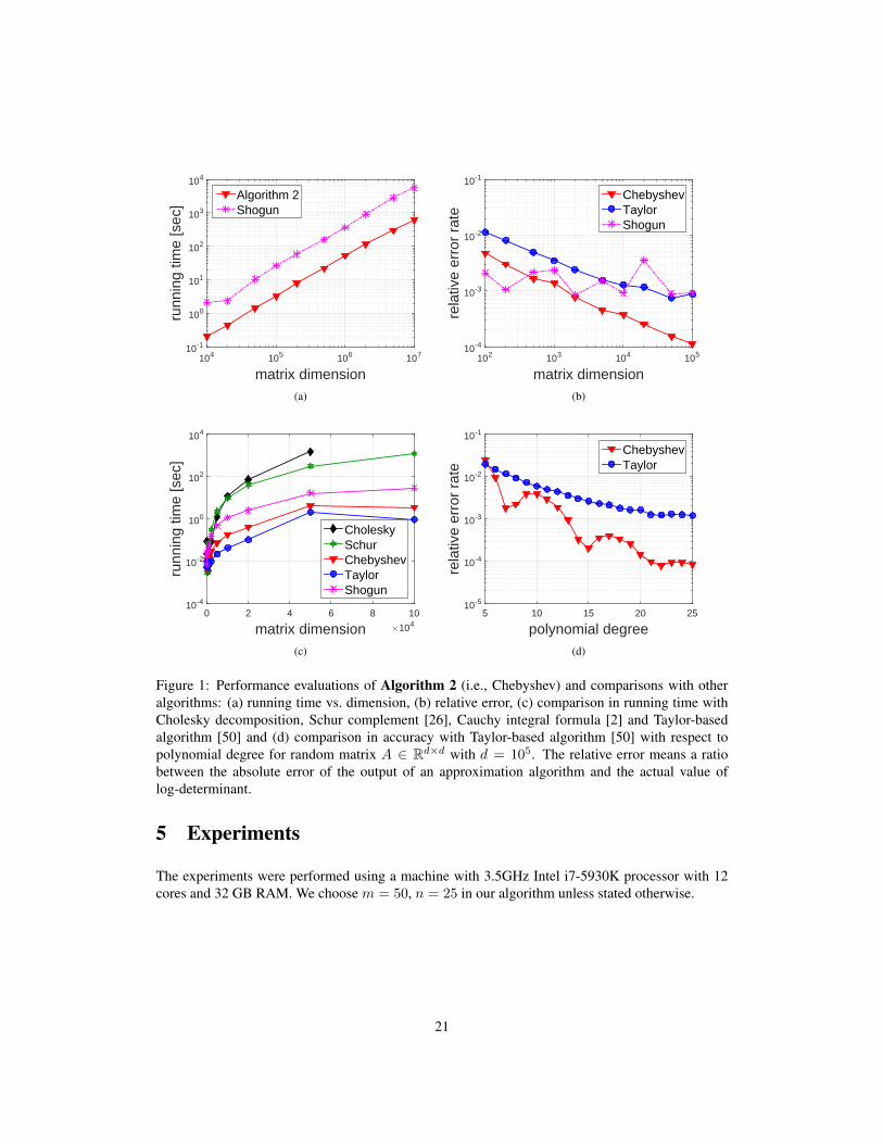
Figure 1: Performance evaluations of Algorithm 2 (i.e., Chebyshev) and comparisons with otheralgorithms: (a) running time vs. dimension, (b) relative error, (c) comparison in running time withCholesky decomposition, Schur complement [26], Cauchy integral formula [2] and Taylor-basedalgorithm [50] and (d) comparison in accuracy with Taylor-based algorithm [50] with respect topolynomial degree for random matrix A ∈ Rd×d with d = 105. The relative error means a ratiobetween the absolute error of the output of an approximation algorithm and the actual value oflog-determinant.

5 Experiments

The experiments were performed using a machine with 3.5GHz Intel i7-5930K processor with 12cores and 32 GB RAM. We choose m = 50, n = 25 in our algorithm unless stated otherwise.

21

5.1 Log-determinant

In this section, we report the performance of our algorithm compared to other methods for computingthe log-determinant of positive definite matrices. We first investigate the empirical performance ofthe proposed algorithm on large sparse random matrices. We generate a random matrix A ∈ Rd×d,where the number of non-zero entries per each row is around 10. We first select non-zero off-diagonal entries in each row with values drawn from the standard normal distribution. To make thematrix symmetric, we set the entries in transposed positions to the same values. Finally, to guaranteepositive definiteness, we set its diagonal entries to absolute row-sums and add a small margin value0.1. Thus, the lower bound for eigenvalues can be chosen as a = 0.1 and the upper bound is set tothe infinite norm of a matrix.

Figure 1 (a) shows the running time of Algorithm 2 from matrix dimension d = 104 to 107. Thealgorithm scales roughly linearly over a large range of matrix sizes as expected. In particular, ouralgorithm is an order of magnitude faster than the recent approach based on Cauchy integral for-mula [2], while it achieves better accuracy as reported in Figure 1 (b).3 It takes only 600 seconds fora matrix of dimension 107 with 108 non-zero entries. In Figure 1 (b), we also compare the relativeaccuracies between our algorithm and that using Taylor expansions [50] with the same samplingnumber m = 50 and polynomial degree n = 25. We see that the Chebyshev interpolation basedmethod more accurate than the one based on Taylor approxiamations. To complete the picture, wealso use a large number of samples for trace estimator, m = 1000, for both algorithms to focuson the polynomial approximation errors. The results are reported in Figure 1 (d), showing thatour algorithm using Chebyshev expansions is superior in accuracy compared to the Taylor-basedalgorithm.

Under the same setup, we also compare the running time of our algorithm with other ones includingCholesky decomposition and Schur complement. The latter was used for sparse inverse covarianceestimation with over a million variables [26] and we run the code implemented by the authors. Therunning time of the algorithms are reported in Figure 1 (c). Our algorithm is dramatically faster thanboth exact methods.

5.2 Other Spectral Functions

In this section, we report the performance of our scheme for four other choices of function f : thetrace of matrix inverse, the Estrada index, the matrix nuclear norm and testing positive definiteness,which correspond to f(x) = 1/x, f(x) = exp(x), f(x) = x1/2 and f(x) = 1

2 (1 + tanh (−αx)),respectively. The detailed algorithm description for each function is given in Section 4. Since therunning time of our algorithms are ‘almost’ independent of the choice of function f , i.e., it is sameas the case f(x) = log x that reported in the previous section, we focus on measuring the accuracyof our algorithm.

In Figure 2, we report the approximation error of our algorithm for the trace of matrix inverse,the Estrada index, the matrix nuclear norm and testing positive definiteness. All experiments wereconducted on random 5000-by-5000 matrices. The particular setup for the different matrix functionsare:

• The input matrix for the trace of matrix inverse is generated in the same way with the log-determinant case in the previous section.

3The method [2] is implemented in the SHOGUN machine learning toolbox, http://www.shogun-toolbox.org.

22

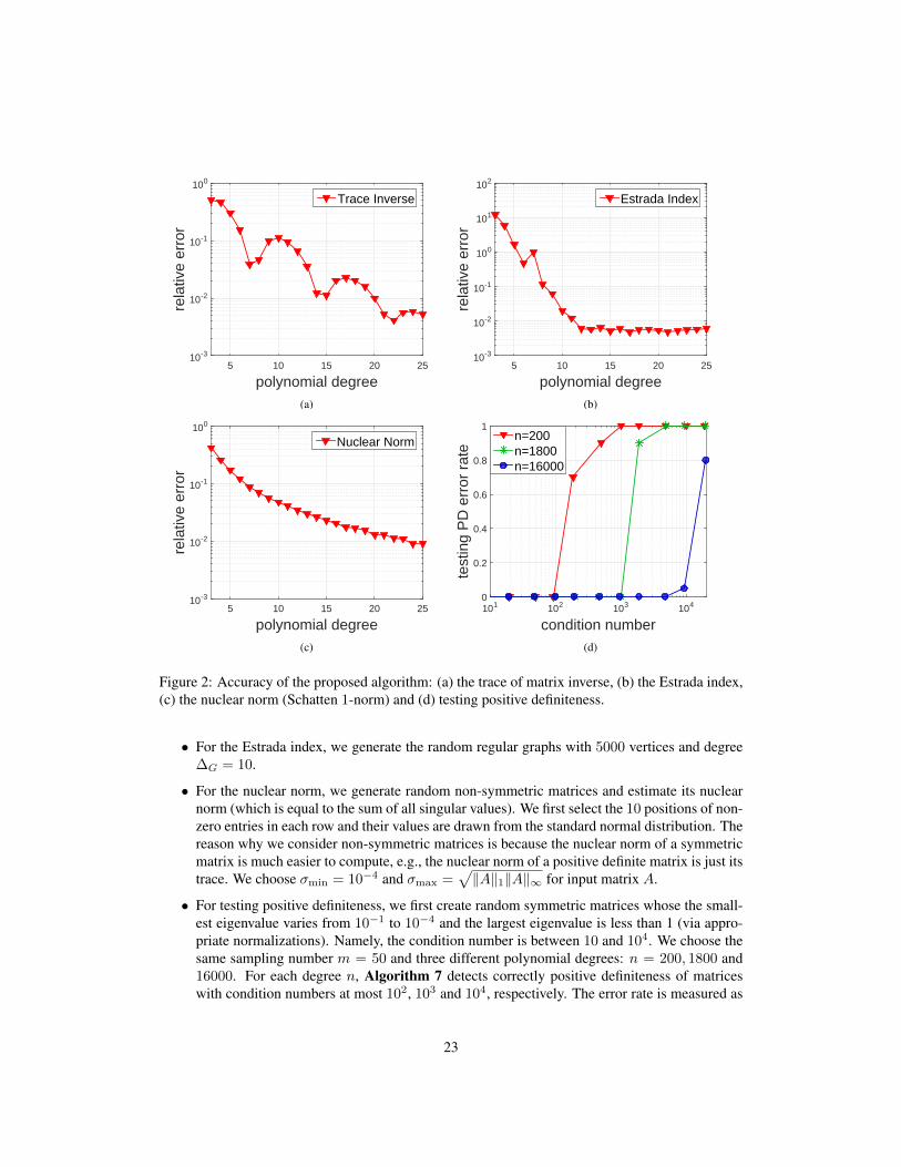
polynomial degree5 10 15 20 25

rela

tive

erro

r

10-3

10-2

10-1

100

Trace Inverse

(a)

polynomial degree5 10 15 20 25

rela

tive

erro

r

10-3

10-2

10-1

100

101

102

Estrada Index

(b)

polynomial degree5 10 15 20 25

rela

tive

erro

r

10-3

10-2

10-1

100

Nuclear Norm

(c)

condition number101 102 103 104

test

ing

PD

err

or r

ate

0

0.2

0.4

0.6

0.8

1n=200n=1800n=16000

(d)

Figure 2: Accuracy of the proposed algorithm: (a) the trace of matrix inverse, (b) the Estrada index,(c) the nuclear norm (Schatten 1-norm) and (d) testing positive definiteness.

• For the Estrada index, we generate the random regular graphs with 5000 vertices and degree∆G = 10.

• For the nuclear norm, we generate random non-symmetric matrices and estimate its nuclearnorm (which is equal to the sum of all singular values). We first select the 10 positions of non-zero entries in each row and their values are drawn from the standard normal distribution. Thereason why we consider non-symmetric matrices is because the nuclear norm of a symmetricmatrix is much easier to compute, e.g., the nuclear norm of a positive definite matrix is just itstrace. We choose σmin = 10−4 and σmax =

√‖A‖1‖A‖∞ for input matrix A.

• For testing positive definiteness, we first create random symmetric matrices whose the small-est eigenvalue varies from 10−1 to 10−4 and the largest eigenvalue is less than 1 (via appro-priate normalizations). Namely, the condition number is between 10 and 104. We choose thesame sampling number m = 50 and three different polynomial degrees: n = 200, 1800 and16000. For each degree n, Algorithm 7 detects correctly positive definiteness of matriceswith condition numbers at most 102, 103 and 104, respectively. The error rate is measured as

23

a ratio of incorrect results among 20 random instances.

For experiment of the trace of matrix inverse, the Estrada index and the nuclear norm, we plot therelative error of the proposed algorithms varying polynomial degrees in Figure 2 (a), (b) and (c),respectively. Each of them achieves less than 1% error with polynomial degree at most n = 25 andsampling number m = 50. Figure 2 (d) shows the results of testing positive definiteness. When n isset according to the conditions number the proposed algorithm is almost always correct in detectingpositive definiteness. For example, if the decision problem involves with the active region Aε forε = 0.02, which is the case that matrices having the condition number at most 100, polynomialdegree n = 200 is enough for the correct decision.

matrix dimension number ofnonzeros

positivedefinite

Algorithm 7n = 200

Algorithm 7n = 1800

Algorithm 7n = 16000

MATLABeigs

MATLABcondest

Chem97ZtZ 2,541 7,361 yes PD PD PD diverge 462.6fv1 9,604 85,264 yes PD PD PD diverge 12.76fv2 9,801 87,025 yes PD PD PD diverge 12.76fv3 9,801 87,025 yes NOT PD NOT PD PD diverge 4420

CurlCurl 0 11,083 113,343 no NOT PD NOT PD NOT PD diverge 6.2×1021barth5 15,606 107,362 no NOT PD NOT PD NOT PD -2.1066 84292

Dubcova1 16,129 253,009 yes NOT PD NOT PD PD 0.0048 2624cvxqp3 17,500 114,962 no NOT PD NOT PD NOT PD diverge 2.2×1016bodyy4 17,546 121,550 yes NOT PD NOT PD PD diverge 1017t3dl e 20,360 20360 yes NOT PD NOT PD PD diverge 6031

bcsstm36 23,052 320,060 no NOT PD NOT PD NOT PD diverge ∞crystm03 24,696 583,770 yes NOT PD PD PD 3.7×10−15 467.7aug2d 29,008 76,832 no NOT PD NOT PD NOT PD -2.8281 ∞

wathen100 30,401 471,601 yes NOT PD NOT PD PD 0.0636 8247aug3dcqp 35,543 128,115 no NOT PD NOT PD NOT PD diverge 4.9×1015wathen120 36,441 565,761 yes NOT PD NOT PD PD 0.1433 4055bcsstk39 46,772 2,060,662 no NOT PD NOT PD NOT PD diverge 3.1×108crankseg 1 52,804 10,614,210 yes NOT PD NOT PD NOT PD diverge 2.2×108blockqp1 60,012 640,033 no NOT PD NOT PD NOT PD -446.636 8.0×105Dubcova2 65,025 1,030,225 yes NOT PD NOT PD PD 0.0012 10411

thermomech TC 102,158 711,558 yes NOT PD PD PD 0.0005 125.5Dubcova3 146,689 3,636,643 yes NOT PD NOT PD PD 0.0012 11482

thermomech dM 204,316 1,423,116 yes NOT PD PD PD 9.1×10−7 125.487pwtk 217,918 11,524,432 yes NOT PD NOT PD NOT PD diverge 5.0×1012bmw3 2 227,362 11,288,630 no NOT PD NOT PD NOT PD diverge 1.2×1020

Table 1: Testing positive definiteness for real-world matrices. Algorithm 7 outputs PD or NOT PD,i.e., the input matrix is either (1) positive definite (PD) or (2) not positive definite or its smallesteigenvalue is in the indifference region (NOT PD). The MATLAB eigs and condest functionsoutput the smallest eigenvalue and an estimate for the condition number of the input matrix, respec-tively.

We tested the proposed algorithm for testing positive definitesss on a collection of real-world ma-trices from the University of Florida Sparse Matrix Collection [13], selecting various symmetricmatrices. We use m = 50 and three choices for n: n = 200, 1800, 16000. The results are reportedin Table 1. We observe that the algorithm is always correct when declaring positive definiteness,but seems to declare indefiniteness when the matrix is too ill-conditioned for it to detect definitenesscorrectly. In addition, with two exceptions (crankseg 1 and pwtk), when n = 16000 the algo-rithm was correct in declaring whether the matrix is positive definite or not. We remark that whilen = 16000 is rather large it is still smaller than the dimension of most of the matrices that weretested (recall that our goal was to develop an algorithm that requires a small number of matrix prod-ucts, i.e., it does not grow with respect to the matrix dimension). We also note that even when thealgorithm fails it still provides useful information about both positive definiteness and the conditionnumber of an input matrix while standard methods such as Cholesky decomposition (as mentioned

24

in Section 4.6) are intractable for large matrices. Furthermore, one can first run an algorithm to es-timate the condition number, e.g., the MATLAB condest function, and then choose an appropriatedegree n. We also run the MATLAB eigs function which is able to estimate the smallest eigenvalueusing iterative methods [28] (hence, it can be used for testing positive definitesss). Unfortunately,the iterative method often does not converge, i.e, residual tolerance may not go to zero, as reportedin Table 1. The advantage of our algorithm compared to the iterative method is to be able to testlarge matrices, without considering such a convergent issue.

5.3 Maximum Likelihood Estimation for GMRF

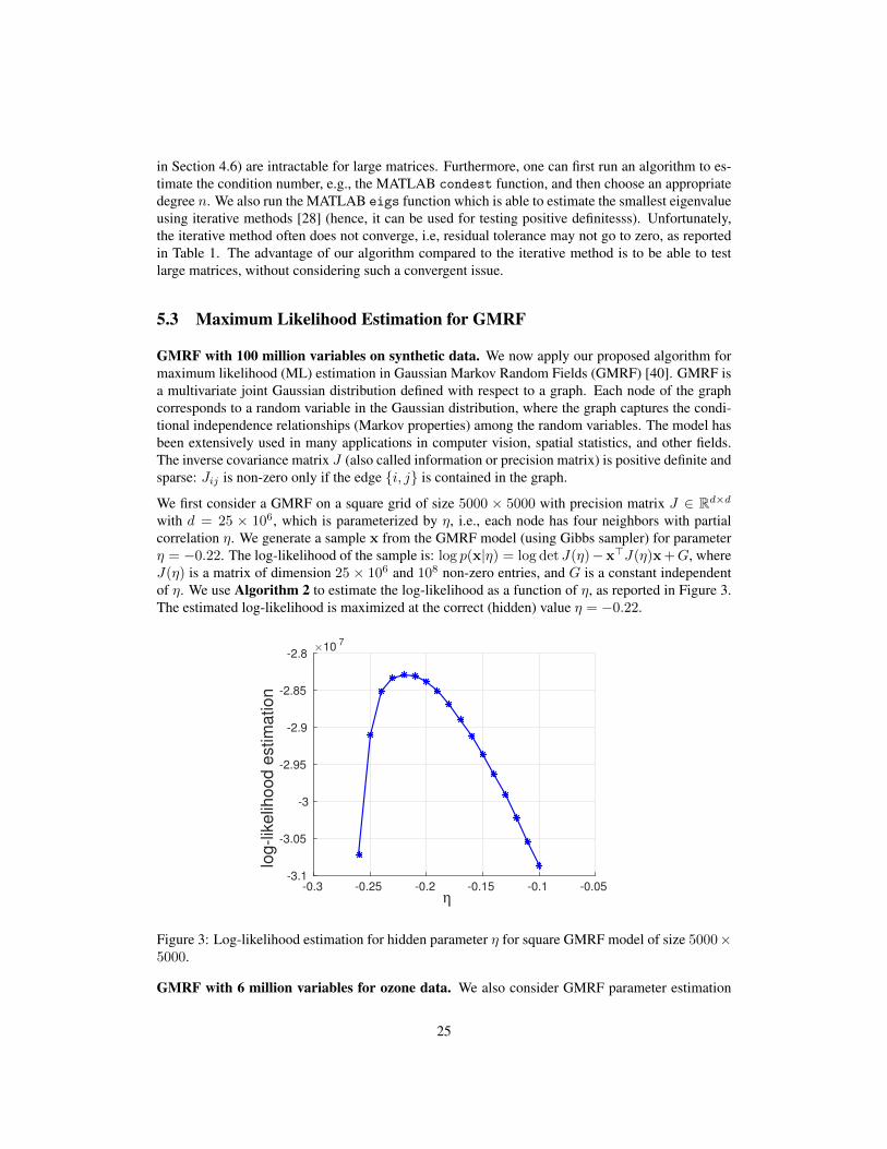
GMRF with 100 million variables on synthetic data. We now apply our proposed algorithm formaximum likelihood (ML) estimation in Gaussian Markov Random Fields (GMRF) [40]. GMRF isa multivariate joint Gaussian distribution defined with respect to a graph. Each node of the graphcorresponds to a random variable in the Gaussian distribution, where the graph captures the condi-tional independence relationships (Markov properties) among the random variables. The model hasbeen extensively used in many applications in computer vision, spatial statistics, and other fields.The inverse covariance matrix J (also called information or precision matrix) is positive definite andsparse: Jij is non-zero only if the edge {i, j} is contained in the graph.

We first consider a GMRF on a square grid of size 5000 × 5000 with precision matrix J ∈ Rd×dwith d = 25 × 106, which is parameterized by η, i.e., each node has four neighbors with partialcorrelation η. We generate a sample x from the GMRF model (using Gibbs sampler) for parameterη = −0.22. The log-likelihood of the sample is: log p(x|η) = log det J(η)−x>J(η)x+G, whereJ(η) is a matrix of dimension 25 × 106 and 108 non-zero entries, and G is a constant independentof η. We use Algorithm 2 to estimate the log-likelihood as a function of η, as reported in Figure 3.The estimated log-likelihood is maximized at the correct (hidden) value η = −0.22.

η-0.3 -0.25 -0.2 -0.15 -0.1 -0.05

log

-lik

elih

oo

d e

stim

atio

n

×107

-3.1

-3.05

-3

-2.95

-2.9

-2.85

-2.8

Figure 3: Log-likelihood estimation for hidden parameter η for square GMRF model of size 5000×5000.

GMRF with 6 million variables for ozone data. We also consider GMRF parameter estimation

25

Figure 4: GMRF interpolation of ozone measurements: (a) original sparse measurements and (b)interpolated values using a GMRF with parameters fitted using Algorithm 2.

from real spatial data with missing values. We use the data-set from [2] that provides satellitemeasurements of ozone levels over the entire earth following the satellite tracks. We use a resolutionof 0.1 degrees in lattitude and longitude, giving a spatial field of size 1681 × 3601, with over 6million variables. The data-set includes 172,000 measurements. To estimate the log-likelihoodin presence of missing values, we use the Schur-complement formula for determinants. Let the

precision matrix for the entire field be J =

(Jo Jo,zJz,o Jz

), where subsets xo and xz denote the

observed and unobserved components of x. The marginal precision matrix of xo is Jo = Jo −Jo,zJ

−1z Jz,o. Its log-determinant is computed as log det(Jo) = log det(J)− log det(Jz) via Schur

complements. To evaluate the quadratic term x′oJoxo of the log-likelihood we need a single linearsolve using an iterative solver. We use a linear combination of the thin-plate model and the thin-membrane models [40], with two parameters α and β: J = αI + (β)Jtp + (1− β)Jtm and obtainML estimates using Algorithm 2. Note that smallest eigenvalue of J is equal to α. We show thesparse measurements in Figure 4 (a) and the GMRF interpolation using fitted values of parametersin Figure 4 (b).

6 Conclusion

Recent years has a seen a surge in the need for various computations on large-scale unstructuredmatrices. The lack of structure poses a significant challenge for traditional decomposition basedmethods. Randomized methods are a natural candidate for such tasks as they are mostly obliviousto structure.

In this paper, we proposed and analyzed a linear-time approximation algorithm for spectral sumsof symmetric matrices, where the exact computation requires cubic-time in the worst case. Fur-thermore, our algorithm is very easy to parallelize since it requires only (separable) matrix-vectormultiplications. We believe that the proposed algorithm will find an important theoretical and com-putational roles in a variety of applications ranging from statistics and machine learning to appliedscience and engineering.

26

Acknowledgement

We thank Peder Olsen for helpful discussions.

References[1] Aravkin, A., Friedlander, M. P., Herrmann, F. J., and Van Leeuwen, T. (2012). Robust inversion,

dimensionality reduction, and randomized sampling. Mathematical Programming, 134(1):101–125.

[2] Aune, E., Simpson, D., and Eidsvik, J. (2014). Parameter estimation in high dimensional Gaus-sian distributions. Statistics and Computing, 24(2):247–263.

[3] Avron, H. (2010). Counting triangles in large graphs using randomized matrix trace estimation.In Workshop on Large-scale Data Mining: Theory and Applications.

[4] Avron, H. and Toledo, S. (2011). Randomized algorithms for estimating the trace of an implicitsymmetric positive semi-definite matrix. Journal of the ACM, 58(2):8.

[5] Bai, Z., Fahey, G., and Golub, G. (1996). Some large-scale matrix computation problems.Journal of Computational and Applied Mathematics, 74(1?2):71 – 89.

[6] Bekas, C., Kokiopoulou, E., and Saad, Y. (2007). An estimator for the diagonal of a matrix.Applied numerical mathematics, 57(11):1214–1229.

[7] Berrut, J. P. and Trefethen, L. N. (2004). Barycentric Lagrange Interpolation. SIAM Review,46(3):501–517.

[8] Boutsidis, C., Drineas, P., Kambadur, P., and Zouzias, A. (2015). A Randomized Algorithmfor Approximating the Log Determinant of a Symmetric Positive Definite Matrix. arXiv preprintarXiv:1503.00374.

[9] Carbo-Dorca, R. (2008). Smooth function topological structure descriptors based on graph-spectra. Journal of Mathematical Chemistry, 44(2):373–378.

[10] Chen, J. (2015). How accurately should I solve linear systems when applying the Hutchinsontrace estimator? IBM Technical Report, RC25581.

[11] Dashti, M. and Stuart, A. M. (2011). Uncertainty quantification and weak approximation of anelliptic inverse problem. SIAM Journal on Numerical Analysis, 49(6):2524–2542.

[12] Davis, J., Kulis, B., Jain, P., Sra, S., and Dhillon, I. (2007). Information-theoretic metriclearning. In ICML.

[13] Davis, T. A. and Hu, Y. (2011). The university of florida sparse matrix collection. ACMTransactions on Mathematical Software (TOMS), 38(1):1–25.

[14] de la Pena, J. A., Gutman, I., and Rada, J. (2007). Estimating the estrada index. Linear Algebraand its Applications, 427(1):70–76.

[15] Dempster, A. P. (1972). Covariance selection. Biometrics, pages 157–175.

[16] Di Napoli, E., Polizzi, E., and Saad, Y. (2013). Efficient estimation of eigenvalue counts in aninterval. arXiv preprint arXiv:1308.4275.

27

[17] Estrada, E. (2000). Characterization of 3d molecular structure. Chemical Physics Letters,319(5):713–718.

[18] Estrada, E. (2007). Topological structural classes of complex networks. Physical Review E,75(1):016103.

[19] Estrada, E. (2008). Atom–bond connectivity and the energetic of branched alkanes. ChemicalPhysics Letters, 463(4):422–425.

[20] Estrada, E. and Hatano, N. (2007). Statistical-mechanical approach to subgraph centrality incomplex networks. Chemical Physics Letters, 439(1):247–251.

[21] Estrada, E. and Rodrıguez-Velazquez, J. A. (2005). Spectral measures of bipartivity in complexnetworks. Physical Review E, 72(4):046105.

[22] Gershgorin, S. A. (1931). Uber die abgrenzung der eigenwerte einer matrix. Izvestiya orRussian Academy of Sciences?, (6):749–754.

[23] Golub, G. H. and Van Loan, C. F. (2012). Matrix computations, volume 3. JHU Press.

[24] Gutman, I., Deng, H., and Radenkovic, S. (2011). The estrada index: an updated survey.Selected Topics on Applications of Graph Spectra, Math. Inst., Beograd, pages 155–174.

[25] Higham, N. J. (2008). Functions of matrices: theory and computation. Siam.

[26] Hsieh, C., Sustik, M. A., Dhillon, I. S., Ravikumar, P. K., and Poldrack, R. (2013). BIG &QUIC: Sparse inverse covariance estimation for a million variables. In Adv. in Neural InformationProcessing Systems, pages 3165–3173.

[27] Hutchinson, M. (1989). A stochastic estimator of the trace of the influence matrix for Lapla-cian smoothing splines. Communications in Statistics-Simulation and Computation, 18(3):1059–1076.

[28] Ipsen, I. C. (1997). Computing an eigenvector with inverse iteration. SIAM review, 39(2):254–291.

[29] Kalantzis, V., Bekas, C., Curioni, A., and Gallopoulos, E. (2013). Accelerating data uncertaintyquantification by solving linear systems with multiple right-hand sides. Numerical Algorithms,62(4):637–653.

[30] Klein, P. and Lu, H.-I. (1996). Efficient approximation algorithms for semidefinite programsarising from max cut and coloring. In Proceedings of the Twenty-eighth Annual ACM Symposiumon Theory of Computing, STOC ’96, pages 338–347, New York, NY, USA. ACM.

[31] Ma, J., Peng, J., Wang, S., and Xu, J. (2013). Estimating the partition function of graphi-cal models using langevin importance sampling. In Proceedings of the Sixteenth InternationalConference on Artificial Intelligence and Statistics, pages 433–441.

[32] Majumdar, A. and Ward, R. K. (2011). An algorithm for sparse mri reconstruction by schattenp-norm minimization. Magnetic resonance imaging, 29(3):408–417.

[33] Malioutov, D. M., Johnson, J. K., and Willsky, A. (2006). Low-rank variance estimation inlarge-scale GMRF models. In IEEE Int. Conf. on Acoustics, Speech and Signal Processing,2006., volume 3, pages III–III. IEEE.

[34] Mason, J. C. and Handscomb, D. C. (2002). Chebyshev polynomials. CRC Press.

28

[35] Moraca, N. (2008). Bounds for norms of the matrix inverse and the smallest singular value.Linear Algebra and its Applications, 429(10):2589–2601.

[36] Nie, F., Huang, H., and Ding, C. H. (2012). Low-rank matrix recovery via efficient schattenp-norm minimization. In AAAI.

[37] Pace, R. K. and LeSage, J. P. (2004). Chebyshev approximation of log-determinants of spatialweight matrices. Computational Statistics & Data Analysis, 45(2):179–196.

[38] Rasmussen, C. E. and Williams, C. (2005). Gaussian processes for machine learning. MITpress.

[39] Roosta-Khorasani, F. and Ascher, U. (2013). Improved bounds on sample size for implicitmatrix trace estimators. arXiv preprint arXiv:1308.2475.

[40] Rue, H. and Held, L. (2005). Gaussian Markov random fields: theory and applications. CRCPress.

[41] Stathopoulos, A., Laeuchli, J., and Orginos, K. (2013). Hierarchical probing for estimat-ing the trace of the matrix inverse on toroidal lattices. SIAM Journal on Scientific Computing,35(5):S299–S322.

[42] Stein, M. L., Chen, J., and Anitescu, M. (2013). Stochastic approximation of score functionsfor Gaussian processes. The Annals of Applied Statistics, 7(2):1162–1191.

[43] Tao, T. and Vu, V. (2010). Random matrices: The distribution of the smallest singular values.Geometric And Functional Analysis, 20(1):260–297.

[44] Tao, T. and Vu, V. H. (2009). Inverse Littlewood-Offord theorems and the condition numberof random discrete matrices. Annals of Mathematics, pages 595–632.

[45] Trefethen, L. N. (2012). Approximation Theory and Approximation Practice (Other Titles inApplied Mathematics). Society for Industrial and Applied Mathematics, Philadelphia, PA, USA.

[46] Van Aelst, S. and Rousseeuw, P. (2009). Minimum volume ellipsoid. Wiley InterdisciplinaryReviews: Computational Statistics, 1(1):71–82.

[47] Wainwright, M. J. and Jordan, M. I. (2006). Log-determinant relaxation for approximate in-ference in discrete Markov random fields. Signal Processing, IEEE Trans. on, 54(6):2099–2109.

[48] Wu, L., Stathopoulos, A., Laeuchli, J., Kalantzis, V., and Gallopoulos, E. (2015). Estimatingthe trace of the matrix inverse by interpolating from the diagonal of an approximate inverse.CoRR, abs/1507.07227.

[49] Xiang, S., Chen, X., and Wang, H. (2010). Error bounds for approximation in Chebyshevpoints. Numerische Mathematik, 116(3):463–491.

[50] Zhang, Y. and Leithead, W. E. (2007). Approximate implementation of the logarithm of thematrix determinant in Gaussian process regression. Journal of Statistical Computation and Sim-ulation, 77(4):329–348.

29