Introduction to Spectral Graph Theory and Graph...
40
Introduction to Spectral Graph Theory and Graph Clustering Chengming Jiang ECS 231 Spring 2016 University of California, Davis 1 / 40
Transcript of Introduction to Spectral Graph Theory and Graph...
Introduction to Spectral Graph Theory and Graph Clustering
Chengming Jiang
ECS 231 Spring 2016
University of California, Davis
1 / 40
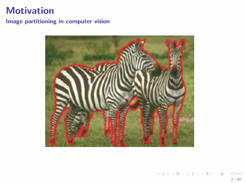
MotivationImage partitioning in computer vision
2 / 40
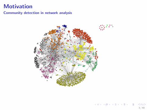
MotivationCommunity detection in network analysis
3 / 40
Outline
I. Graph and graph LaplacianI GraphI Weighted graphI Graph Laplacian
II. Graph clusteringI Graph clusteringI Normalized cutI Spectral clustering
4 / 40
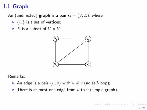
I.1 Graph
An (undirected) graph is a pair G = (V,E), where
I {vi} is a set of vertices;
I E is a subset of V × V .
Remarks:
I An edge is a pair {u, v} with u 6= v (no self-loop);
I There is at most one edge from u to v (simple graph).
5 / 40
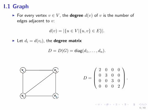
I.1 Graph
I For every vertex v ∈ V , the degree d(v) of v is the number ofedges adjacent to v:
d(v) = |{u ∈ V |{u, v} ∈ E}|.
I Let di = d(vi), the degree matrix
D = D(G) = diag(d1, . . . , dn).
D =
2 0 0 00 3 0 00 0 3 00 0 0 2
.
6 / 40
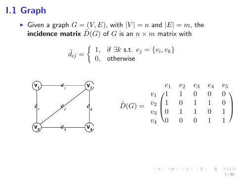
I.1 Graph
I Given a graph G = (V,E), with |V | = n and |E| = m, theincidence matrix D(G) of G is an n×m matrix with
dij =
{1, if ∃k s.t. ej = {vi, vk}0, otherwise
D(G) =
e1 e2 e3 e4 e5
v1 1 1 0 0 0v2 1 0 1 1 0v3 0 1 1 0 1v4 0 0 0 1 1
7 / 40
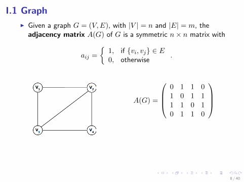
I.1 Graph
I Given a graph G = (V,E), with |V | = n and |E| = m, theadjacency matrix A(G) of G is a symmetric n× n matrix with
aij =
{1, if {vi, vj} ∈ E0, otherwise
.
A(G) =
0 1 1 01 0 1 11 1 0 10 1 1 0
8 / 40
I.2 Weighted graph
A weighted graph is a pair G = (V,W ) where
I V = {vi} is a set of vertices and |V | = n;
I W ∈ Rn×n is called weight matrix with
wij =
{wji ≥ 0 if i 6= j0 if i = j
The underlying graph of G is G = (V,E) with
E = {{vi, vj}|wij > 0}.
I If wij ∈ {0, 1}, W = A, the adjacency matrix of G.
I Since wii = 0, there is no self-loops in G.
9 / 40
I.2 Weighted graph
I For every vertex vi ∈ V , the degree d(vi) of vi is the sum ofthe weights of the edges adjacent to vi:
d(vi) =
n∑j=1
wij .
I Let di = d(vi), the degree matrix
D = D(G) = diag(d1, . . . , dn).
Remark:Let d = diag(D) and denote 1 = (1, . . . , 1)T , then d = W1.
10 / 40
I.2 Weighted graph
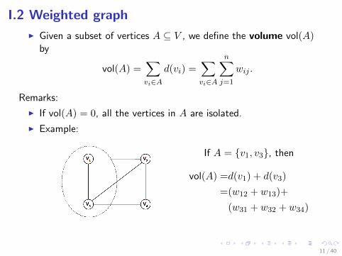
I Given a subset of vertices A ⊆ V , we define the volume vol(A)by
vol(A) =∑vi∈A
d(vi) =∑vi∈A
n∑j=1
wij .
Remarks:
I If vol(A) = 0, all the vertices in A are isolated.
I Example:
If A = {v1, v3}, then
vol(A) =d(v1) + d(v3)
=(w12 + w13)+
(w31 + w32 + w34)
11 / 40
I.2 Weighted graph
I Given two subsets of vertices A,B ⊆ V , we define the linkslinks(A,B) by
links(A,B) =∑
vi∈A,vj∈Bwij .
Remarks:
I A and B are not necessarily distinct;
I Since W is symmetric, links(A,B) = links(B,A);
I vol(A) = links(A, V ).
12 / 40
I.2 Weighted graph
I The quantity cut(A) is defined by
cut(A) = links(A, V −A).
I The quantity assoc(A) is defined by
assoc(A) = links(A,A).
Remarks:
I cut(A) measures how many links escape from A;
I assoc(A) measures how many links stay within A;
I cut(A) + assoc(A) = vol(A).
13 / 40
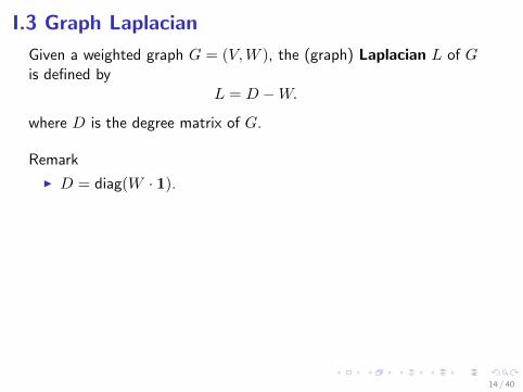
I.3 Graph Laplacian
Given a weighted graph G = (V,W ), the (graph) Laplacian L of Gis defined by
L = D −W.
where D is the degree matrix of G.
Remark
I D = diag(W · 1).
14 / 40
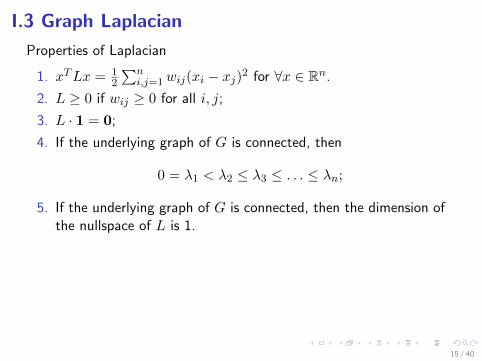
I.3 Graph Laplacian
Properties of Laplacian
1. xTLx = 12
∑ni,j=1wij(xi − xj)2 for ∀x ∈ Rn.
2. L ≥ 0 if wij ≥ 0 for all i, j;
3. L · 1 = 0;
4. If the underlying graph of G is connected, then
0 = λ1 < λ2 ≤ λ3 ≤ . . . ≤ λn;
5. If the underlying graph of G is connected, then the dimension ofthe nullspace of L is 1.
15 / 40
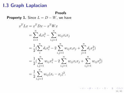
I.3 Graph Laplacian
ProofsProperty 1. Since L = D −W , we have
xTLx = xTDx− xTWx
=
n∑i=1
dix2i −
n∑i,j=1
wijxixj
=1
2(
n∑i
dix2i − 2
n∑i,j=1
wijxixj +
n∑j=1
djx2j )
=1
2(
n∑i,j=1
wijx2i − 2
n∑i,j=1
wijxixj +
n∑i,j=1
wijx2j )
=1
2
n∑i,j=1
wij(xi − xj)2.
16 / 40
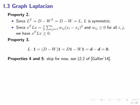
I.3 Graph Laplacian
Property 2.
I Since LT = D −W T = D −W = L, L is symmetric.
I Since xTLx = 12
∑ni,j=1wij(xi − xj)2 and wij ≥ 0 for all i, j,
we have xTLx ≥ 0.
Property 3.
L · 1 = (D −W )1 = D1−W1 = d− d = 0.
Properties 4 and 5: skip for now, see §2.2 of [Gallier’14].
17 / 40
Outline
I. Graph and graph LaplacianI GraphI Weighted graphI Graph Laplacian
II. Graph clusteringI Graph clusteringI Normalized cutI Spectral clustering
18 / 40
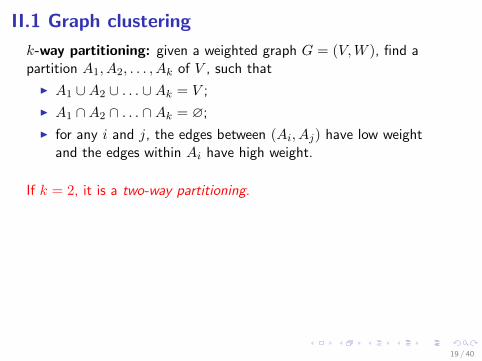
II.1 Graph clustering
k-way partitioning: given a weighted graph G = (V,W ), find apartition A1, A2, . . . , Ak of V , such that
I A1 ∪A2 ∪ . . . ∪Ak = V ;
I A1 ∩A2 ∩ . . . ∩Ak = ∅;
I for any i and j, the edges between (Ai, Aj) have low weightand the edges within Ai have high weight.
If k = 2, it is a two-way partitioning.
19 / 40
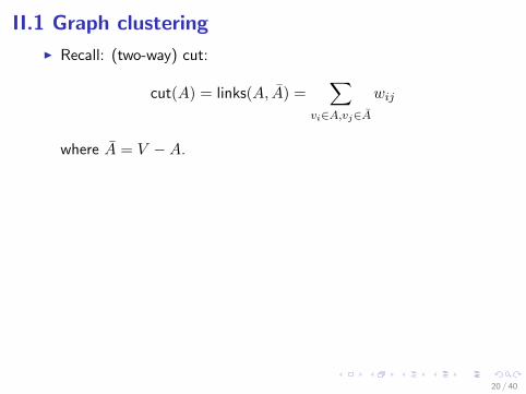
II.1 Graph clustering
I Recall: (two-way) cut:
cut(A) = links(A, A) =∑
vi∈A,vj∈A
wij
where A = V −A.
20 / 40
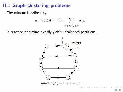
II.1 Graph clustering problems
The mincut is defined by
min cut(A) = min∑
vi∈A,vj∈A
wij .
In practice, the mincut easily yields unbalanced partitions.
min cut(A) = 1 + 2 = 3;
21 / 40
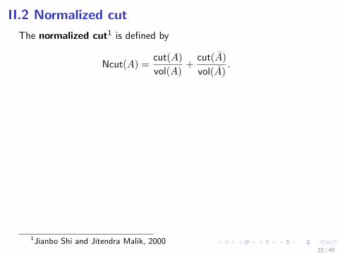
II.2 Normalized cut
The normalized cut1 is defined by
Ncut(A) =cut(A)
vol(A)+
cut(A)
vol(A).
1Jianbo Shi and Jitendra Malik, 200022 / 40
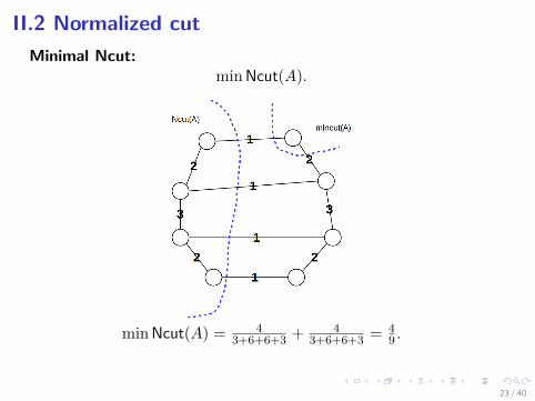
II.2 Normalized cut
Minimal Ncut:min Ncut(A).
min Ncut(A) = 43+6+6+3 + 4
3+6+6+3 = 49 .
23 / 40
II.2 Normalized cut
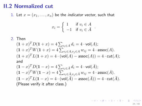
1. Let x = (x1, . . . , xn) be the indicator vector, such that
xi =
{1 if vi ∈ A−1 if vi ∈ A
.
2. Then(1 + x)TD(1 + x) = 4
∑vi∈A di = 4 · vol(A);
(1 + x)TW (1 + x) = 4∑
vi∈A,vj∈Awij = 4 · assoc(A).
(1 + x)TL(1 + x) = 4 · (vol(A)− assoc(A)) = 4 · cut(A);and(1− x)TD(1− x) = 4
∑vi∈A di = 4 · vol(A);
(1− x)TW (1− x) = 4∑
vi∈A,vj∈Awij = 4 · assoc(A).
(1− x)TL(1− x) = 4 · (vol(A)− assoc(A)) = 4 · cut(A).(Please verify it after class.)
24 / 40
II.2 Normalized cut
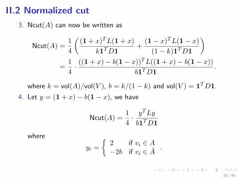
3. Ncut(A) can now be written as
Ncut(A) =1
4
((1 + x)TL(1 + x)
k1TD1+
(1− x)TL(1− x)
(1− k)1TD1
)=
1
4· ((1 + x)− b(1− x))TL((1 + x)− b(1− x))
b1TD1.
where k = vol(A)/vol(V ), b = k/(1− k) and vol(V ) = 1TD1.
4. Let y = (1 + x)− b(1− x), we have
Ncut(A) =1
4· y
TLy
b1TD1
where
yi =
{2 if vi ∈ A−2b if vi ∈ A
.
25 / 40
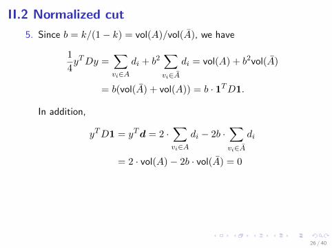
II.2 Normalized cut
5. Since b = k/(1− k) = vol(A)/vol(A), we have
1
4yTDy =
∑vi∈A
di + b2∑vi∈A
di = vol(A) + b2vol(A)
= b(vol(A) + vol(A)) = b · 1TD1.
In addition,
yTD1 = yTd = 2 ·∑vi∈A
di − 2b ·∑vi∈A
di
= 2 · vol(A)− 2b · vol(A) = 0
26 / 40
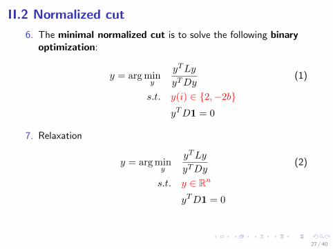
II.2 Normalized cut
6. The minimal normalized cut is to solve the following binaryoptimization:
y = arg miny
yTLy
yTDy(1)
s.t. y(i) ∈ {2,−2b}yTD1 = 0
7. Relaxation
y = arg miny
yTLy
yTDy(2)
s.t. y ∈ Rn
yTD1 = 0
27 / 40
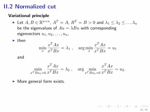
II.2 Normalized cut
Variational principle
I Let A,B ∈ Rn×n, AT = A, BT = B > 0 and λ1 ≤ λ2 ≤ . . . λnbe the eigenvalues of Au = λBu with correspondingeigenvectors u1, u2, . . . , un,
I then
minx
xTAx
xTBx= λ1 , arg min
x
xTAx
xTBx= u1
and
minxTBu1=0
xTAx
xTBx= λ2 , arg min
xTBu1=0
xTAx
xTBx= u2.
I More general form exists.
28 / 40
II.2 Normalized cut
I For the matrix pair (L,D), it is known that (λ1, y1) = (0,1).
I By the variational principle, the relaxed minimal Ncut (2) isequivalent to finding the second smallest eigenpair (λ2, y2) of
Ly = λDy (3)
Remarks:
I L is extremely sparse and D is diagonal;
I Precision requirement for eigenvectors is low, say O(10−3).
29 / 40
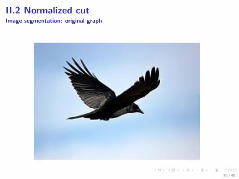
II.2 Normalized cutImage segmentation: original graph
30 / 40
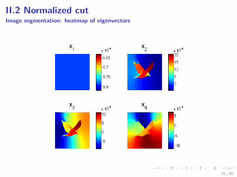
II.2 Normalized cutImage segmentation: heatmap of eigenvectors
31 / 40
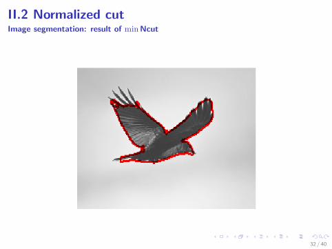
II.2 Normalized cutImage segmentation: result of minNcut
32 / 40
II.3 Spectral clusteringNcut remaining issues
I Once the indicator vector is computed, how to search thesplitting point that the resulting partition has the minimalNcut(A) value?
I How to use the extreme eigenvectors to do the k-waypartitioning?
The above two problems are addressed in spectral clusteringalgorithm.
33 / 40
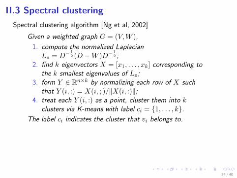
II.3 Spectral clustering
Spectral clustering algorithm [Ng et al, 2002]
Given a weighted graph G = (V,W ),
1. compute the normalized LaplacianLn = D−
12 (D −W )D−
12 ;
2. find k eigenvectors X = [x1, . . . , xk] corresponding tothe k smallest eigenvalues of Ln;
3. form Y ∈ Rn×k by normalizing each row of X suchthat Y (i, :) = X(i, ; )/‖X(i, :)‖;
4. treat each Y (i, :) as a point, cluster them into kclusters via K-means with label ci = {1, . . . , k}.
The label ci indicates the cluster that vi belongs to.
34 / 40
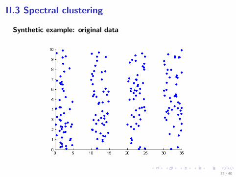
II.3 Spectral clustering
Synthetic example: original data
35 / 40
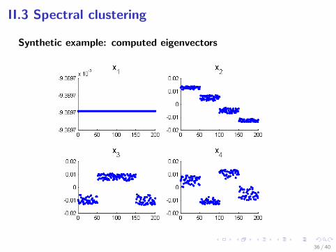
II.3 Spectral clustering
Synthetic example: computed eigenvectors
36 / 40
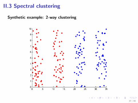
II.3 Spectral clustering
Synthetic example: 2-way clustering
37 / 40
II.3 Spectral clustering
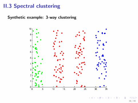
Synthetic example: 3-way clustering
38 / 40
II.3 Spectral clustering
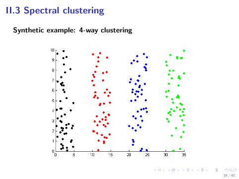
Synthetic example: 4-way clustering
39 / 40
References
1. Jean Gallier, Notes on elementary spectral graph theoryapplications to graph clustering using normalized cuts, 2013.
2. Jianbo Shi and Jitendra Malik, Normalized cuts and imagesegmentation, 2000.
3. Andrew Y Ng, Michael I. Jordan and Yair Weiss, On spectralclustering: Analysis and an algorithm, 2001
40 / 40