
Chapter 16 Model Predictive Control. Single Loop Controllers.
190
Chapter 16 Model Predictive Control
-
Upload
evelyn-snow -
Category
Documents
-
view
234 -
download
1
Transcript of Chapter 16 Model Predictive Control. Single Loop Controllers.

Chapter 16
Model Predictive Control

Single Loop Controllers
y 1
y 2u 2
u 1G C1
+
-G C2
y 1,sp
y 2,sp
G 11 (s)
++
G 21 (s)
G 12 (s)
G 22 (s)
++
Control Loop 1
Control Loop 2
+ -
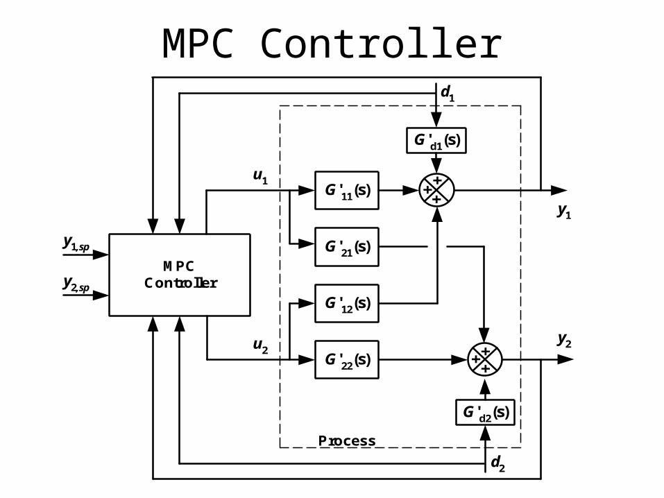
MPC Controller
y1
y2u2
u1
y1,sp
y2,sp
G'11(s)
G'21(s)
G'12(s)
G'22(s)
+ +
+ +
MPCController
Process
+
+
G'd1(s)
d1
G'd2(s)
d2

Model Predictive Control
• Most popular form of multivariable control.
• Effectively handles complex sets of constraints.
• Has an LP on top of it so that it controls against the most profitable set of constraints.
• Several types of industrial MPC but DMC is the most widely used form.

DMC is based on Step Response Models
• Allow the development of empirical input/output process models.
• The coefficients correspond to the step response behavior of the process
0
ˆ( )
( )i
i
y ta
u t

Example of a SRM
•• t i u y(t) ai
• 0 0 1 0 0
• 1 1 0 0 0
• 2 2 0 0.63 0.63
• 3 3 0 0.87 0.87
• 4 4 0 0.95 0.95
• 5 5 0 0.98 0.98
• 6 6 0 0.99 0.99
• 7 7 0 1.00 1.00
• 8 8 0 1.00 1.00

Open-Loop Step Test for Thermal Mixer
48
49
50
51
0 20 40 60 80 100Time (s)
Te
mp
era
ture
(ºC
)

SRM for the Thermal Mixer (u=0.05)i ti yi ai
0 5 50.00 0.0 0.0
1 10 49.77 -0.23 -4.68
2 15 49.35 -0.65 -13.0
3 20 49.08 -0.92 -18.4
4 25 48.94 -1.06 -21.2
5 30 48.87 -1.13 -22.6
6 35 48.84 -1.16 -23.2
7 40 48.83 -1.17 -23.5
8 45 48.82 -1.18 -23.7
9 50 48.82 -1.18 -23.7
ˆiy

Example of SRM Applied to a Process with Complex Dynamics
1.5
1.7
1.9
2.1
2.3
2.5
0 100 200 300 400Time
y •
•
•
••
••
•a1 a2a5
a3
a6
a7a8
a4
• SRM: [0 0 -0.3 -0.1 0.05 0.1 0.2 0.3 . . .]
Complex Dynamics
• An integrating process (e.g., a level) is modeled the same except that the Tss is based on attaining a constant slope (i.e., a constant ramp rate).
• An integrating variable is referred to as a “ramp variable”.

SRM for Ramp Function
Time
u=1
• ••
••
y0
Tss
y1
y2
y3
y4
Ts

Using SRM to Calculate y(t)• Given: SRM: [0 0.4 0.8 0.9 1.0]
– y0=5 u=5 Ts=20 sec
• Solve for y(t):– y = y0 + u SRM
– y1=5 + 5×0 = 5; y2 = 5 + 5×0.4 = 7;
– y3 = 5 +5×0.8 = 9; y4 = 5 + 5×.9 = 9.5
– y5 = 5 + 5×1 = 10 or in vector form
– y = [5 7 9 9.5 10 10 10 …]
– y(20 s)=5; y(40 s)=7; y(60 s)=9; y(80 s)=9.5
– y(100 s)=10; y(120 s)=10; y(140 s)=10 ...

Class Exercise
• Given: SRM: [0 0.4 0.8 0.9 1.0]– y0=5 u=-2 Ts=20 sec
• Solve for y(t):

Solution to Class Exercise
• Given: SRM: [0 0.4 0.8 0.9 1.0]– y0=5 u=-2 Ts=20 sec
• Solve for y(t):– y = y0 + u SRM
– y1=5 + -2×0 = 5; y2 = 5 + -2×0.4 = 4.2;
– y3 = 5 +-2×0.8 = 3.4; y4 = 5 + -2×.9 =3.2
– y5 = 5 + -2×1 = 3 or in vector form
– y = [5 4.2 3.4 3.2 3 3 3 …]
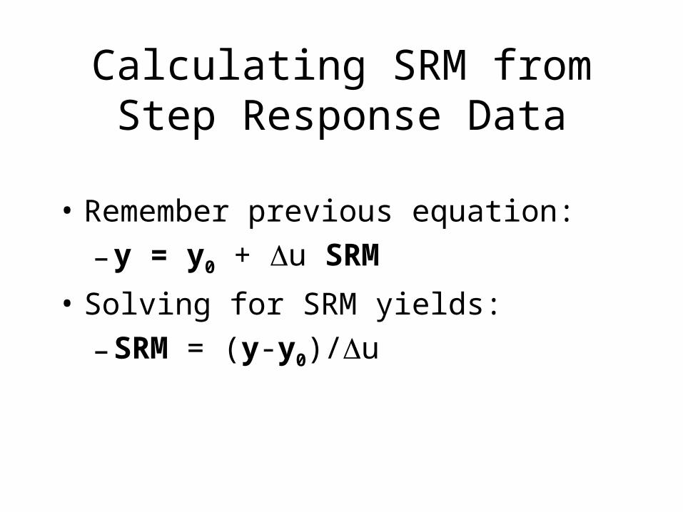
Calculating SRM from Step Response Data
• Remember previous equation:
– y = y0 + u SRM
• Solving for SRM yields:
– SRM = (y-y0)/u
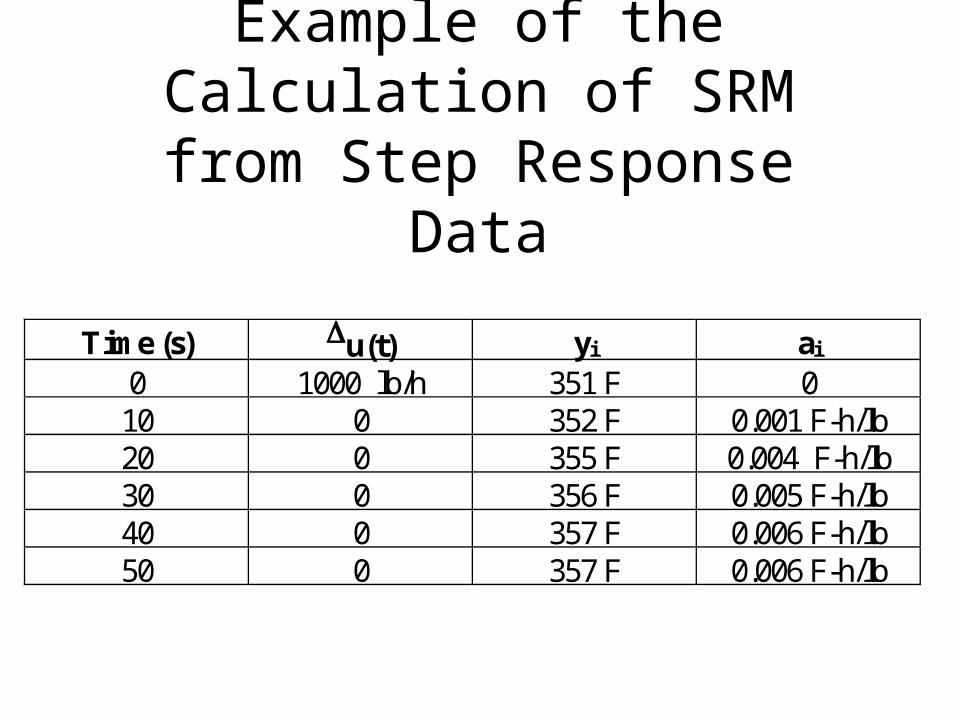
Example of the Calculation of SRM from Step Response Data
Time (s) u(t) yi ai
0 1000 lb/h 351 F 010 0 352 F 0.001 F-h/lb20 0 355 F 0.004 F-h/lb30 0 356 F 0.005 F-h/lb40 0 357 F 0.006 F-h/lb50 0 357 F 0.006 F-h/lb

Class Exercise for the Calculation of the SRM from
Step Response Data
Time (s) u(t) yi ai
0 500 lb/h 55 psig10 0 53 psig20 0 48 psig30 0 46 psig40 0 45 psig50 0 45 psig
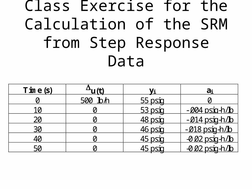
Class Exercise for the Calculation of the SRM from
Step Response Data
Time (s) u(t) yi ai
0 500 lb/h 55 psig 010 0 53 psig -.004 psig-h/lb20 0 48 psig -.014 psig-h/lb30 0 46 psig -.018 psig-h/lb40 0 45 psig -0.02 psig-h/lb50 0 45 psig -0.02 psig-h/lb

Simulation Demonstration
• A thermal mixing process mixes two streams with different temperatures (25ºC and 75ºC) to produce a product (about 50ºC).
• Consider a 10% increase (0.05 kg/s) increase in the flow rate of colder stream.
• Develop SRM from step response.

Step Test Result and SRM
Time (s) Outlet Temperature (ºC) SRM Coefficients (ºC-s/kg)5 50
12 49.77 -4.6819 49.35 -13.026 49.08 -18.433 48.94 -21.240 48.87 -22.647 48.84 -23.254 48.82 -23.561 48.816 -23.768 48.813 -23.775 48.811 -23.8
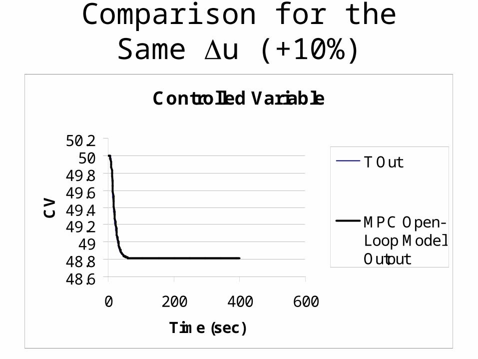
Comparison for the Same u (+10%)
Controlled Variable
48.648.8
4949.249.449.649.8
5050.2
0 200 400 600
Time (sec)
CV
T Out
MPC Open-Loop ModelOutput

Comparison for the Same u (-10%)
Controlled Variable
49.5
50
50.5
51
51.5
0 200 400 600
Time (sec)
CV
T Out
MPC Open-LoopModel Output

Demonstration Conclusions
• MPC model agrees closely for the same step input change, but shows significant mismatch for a different size of input change due to process nonlinearity.

Nonlinear Effects
• This SRM will not accurately represent negative changes in the MV or different magnitude MV changes due to process nonlinearity.
• Therefore, a better way to develop a SRM is to make a number of MV changes with different magnitude and directions and average the results to get the SRM.

SRM’s for Different Size u’s
+10% +5% -5% -10% Averageu 0.05 0.025 -0.025 -0.05 -a1 -4.68 -4.70 -4.73 -4.75 -4.72a2 -13.0 -13.2 -13.4 -13.5 -13.3a3 -18.4 -18.7 -19.2 -19.5 -19.0a4 -21.2 -21.6 -22.4 -22.8 -22.0a5 -22.6 -23.0 -24.0 -24.5 -23.3a6 -23.2 -23.7 -24.8 -25.4 -24.3a7 -23.5 -24.1 -25.2 -25.8 -24.7a8 -23.7 -24.2 -25.4 -26.1 -24.9a9 -23.7 -24.3 -25.5 -26.2 -24.9a10 -23.8 -24.4 -25.6 -26.3 -25.0

Another Approach
• Use the average ai’s

Using Average ai’s for u=+10%
Time F1 T Out MPC Open-Loop Model OutputT1 F1 S.P.0 0.5 50 50 25 0.51 0.5 50 50 25 0.52 0.5 50 50 25 0.53 0.5 50 50 25 0.54 0.5 50 50 25 0.55 0.5 50 50 25 0.56 0.514376 49.99804 50 25 0.557 0.524619 49.98688 49.96629 25 0.558 0.531917 49.96313 49.93257 25 0.559 0.537116 49.92698 49.89886 25 0.55

Using Average ai’s for u=-10%
Time F1 T Out MPC Open-Loop Model OutputT1 F1 S.P.0 0.5 50 50 25 0.51 0.5 50 50 25 0.52 0.5 50 50 25 0.53 0.5 50 50 25 0.54 0.5 50 50 25 0.55 0.5 50 50 25 0.56 0.485624 50.00196 50 25 0.457 0.475381 50.01314 50.03371 25 0.45

Using Average ai’s for u=+5%
Controlled Variable
49.2
49.4
49.6
49.8
50
50.2
0 200 400 600
Time (sec)
CV
T Out
MPC Open-Loop ModelOutput

Relation to MPC Model Identification
• Developing SRM’s that represent an “average” response is the basis of good MPC models.

Class Exercise
• Using the composition mixer simulator (CMIXER), use a +5% step input change (0.025 kg/min) to generate a SRM for this process
• First, implement the step input change• Next, determine the model interval• Then, calculate the SRM coefficients• Finally, compare simulator result to MPC model
prediction for u (+10% to -10%)

SRM Summary
• SRM’s represent the dynamic behavior of a dependent variable (output variable) for a process for a unit step change in an input.
• SRM’s are empirical models that are flexible enough to model complex dynamics
• SRM’s are linear approximations of process behavior and can be estimated using step responses for the process.

SISO MPC Controller
Application of SRM for a Series of Input Changes

A Series of Input Changes
• Definition of the SRM is based on a single step input change.
• But feedback control requires a large number of changes to the input variables.
• To use a SRM to predict the output behavior for a series of input changes, linear superposition is assumed, i.e., the process response is equal to the sum of the individual step responses.

Superposition of Two Step Input Changes
Time
uu1
u2
u2
u1
Combined Response

Superposition of Two Step Input Changes
Time
u
u1u2
u2
u1 Combined Response

Equation Form for Two Sequential Input Changes
• Consider the the response of a process to two step input changes separately
0 1
1 0 0 1
2 0 0 2 2 0 1 1
3 0 0 3 3 0 1 2
4 0 0 4 4 0 1 3
is applied at 0 is applied at
. .
. .
. .
su t u t T
y y u a
y y u a y y u a
y y u a y y u a
y y u a y y u a
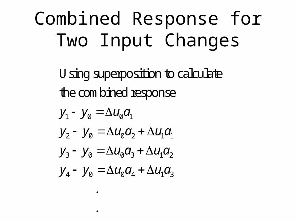
Combined Response for Two Input Changes
1 0 0 1
2 0 0 2 1 1
3 0 0 3 1 2
4 0 0 4 1 3
Using superposition to calculate
the combined response
.
.
.
y y u a
y y u a u a
y y u a u a
y y u a u a

Combined Response for a Series of 4 Input Changes
1 0 0 1
2 0 0 2 1 1
3 0 0 3 1 2 2 1
4 0 0 4 1 3 2 2 3 1
5 0 0 5 1 4 2 3 3 2 4 1
Using superposition to calculate
the combined response
y y u a
y y u a u a
y y u a u a u a
y y u a u a u a u a
y y u a u a u a u a u a

Matrix Form for Combined Response for a Series of 4 Input Changes
1 0 1
2 0 2 10
3 0 3 2 11
4 0 4 3 2 12
5 0 4 4 3 23
6 0 4 4 4 3
7 0 4 4 4 4
0 0 0
0 0
0
y y a
y y a au
y y a a au
y y a a a au
y y a a a au
y y a a a a
y y a a a a

The Dynamic Matrix
• The Dynamic Matrix determines the dynamic response of the process to a series of input changes, nc, for a prediction horizon of np steps into the future.
• The dynamic Matrix is constructed from the coefficients of the SRM
• A is np×nc; SRM is m (this case has 4 inputs and 7 output predictions)
1
2 1
3 2 1
4 3 2 1
4 4 3 2
4 4 4 3
4 4 4 4
0 0 0
0 0
0
a
a a
a a a
a a a a
a a a a
a a a a
a a a a
A

Zero’s in Dynamic Matrix
• Where do they come from?
• Consider the first row: y1 is cannot be affected by u1, u2, and u3 because y1 is measured before u1, u2, and u3 are applied.
• Likewise, y2 is cannot be affected by u2 and u3

The Matrix Form of the Generalized Model Equation
1 0
2 0
where .
.
.
y y
y y
y = A u y

Dynamic Matrix Example
SRM: (0.1 0.5 0.9 1.0) ; 1.5
0.1 0 0 0
0.5 0.1 0 0
0.9 0.5 0.1 0
1.0 0.9 0.5 0.1
1.0 1.0 0.9 0.5
1.0 1.0 1.0 0.9
c pn m n m
A

Class Exercise
SRM: (0.3 1.0)
is a 3 by 3 matrix (i.e., =1.5
and )
p
c
n m
n m
A

Solution to Class Exercise
SRM: (0.3 1.0)
0.3 0
1.0 0.3
1.0 1.0
A

SISO MPC Controller
Prediction Vector

Previous Inputs Affect Future Response of the Process
-10 -5 0 5 10Time
u
Past Inputs
Future Inputs

Previous Inputs Affect Future Response of the Process
-10 -5 0 5 10Time
y
Past Behavior
Future Prediction
Setpoint

Prediction Vector
• The prediction vector, yP, contains the combined effect of the previous input changes on the future values of the output variable.
• The prediction vector is calculated from the product of the previous input changes and the prediction matrix, which is constructed using the coefficients of the SRM.

Process Model
• The future values of the output variable are equal to the sum of the contribution from previous inputs (prediction vector) and the contribution from future change in the input variable:
where is the vector of input changes
Py = y + A u
u
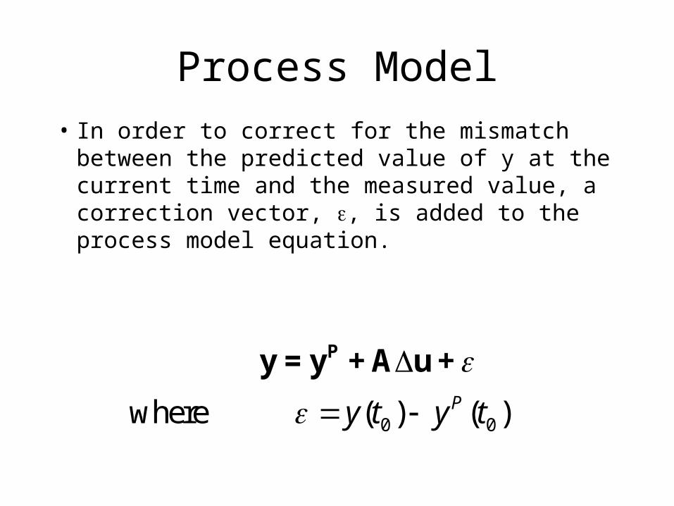
Process Model
• In order to correct for the mismatch between the predicted value of y at the current time and the measured value, a correction vector, , is added to the process model equation.
0 0where ( ) ( )Py t y t
Py = y + A u +
Correction for Mismatch in Ramp Variable
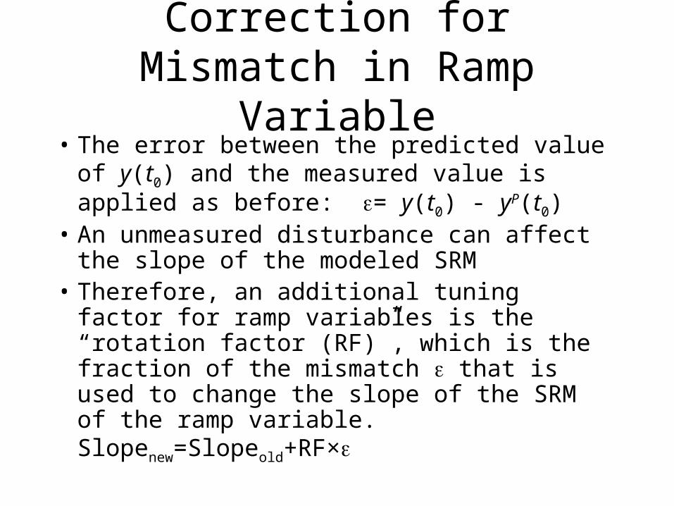
• The error between the predicted value of y(t0) and the measured value is applied as before: = y(t0) - yP(t0)
• An unmeasured disturbance can affect the slope of the modeled SRM
• Therefore, an additional tuning factor for ramp variables is the “rotation factor (RF)”, which is the fraction of the mismatch that is used to change the slope of the SRM of the ramp variable. Slopenew=Slopeold+RF×
SISO MPC Controller
DMC Controller

Development of DMC Control Law
2
2
Minimize the error from setpoint:
( )
Substituting for
( )
sp ii
i
Psp i i
i
Min y y
y
y y A u

DMC Control Law
2
Define
( )
DMC Control Law:
Pi sp i
i ii
E y y
E A u
T -1 Tu = (A A) A E

Analysis of DMC Controller
• (ATA)-1AT is a constant matrix that is determined explicitly from the coefficients of the SRM.
• If you double the number of coefficients in the SRM, you will increase the number of terms in the dynamic matrix by a factor of 4
• E takes into account changes in the setpoint, the influence of previous inputs, and the correction for model mismatch.
• A full set of future moves are determine by this control law at each control interval.

Moving Horizon Controller
-10 -5 0 5 10Time
y
Past Behavior
Future Prediction
Setpoint

Moving Horizon Controller
• Even though the DMC controller calculates a series of future moves, only the first of the calculated moves is actually implemented.
• The next time the controller is called (Ts later), a new series of moves is calculated, but only the first is applied.
• If the SRM were perfect, the subsequent set of first moves would be equal to the first series of moves calculated by the DMC controller.

SISO MPC Controller
Implementation Details

Implementation Details
• Choose Ts based on when new information is available on the CV. E.g., analyzer update. For temperature sensor, use Ts=10-15 s.
• Model horizon: m= Tss / Ts (normally set m=60-90 coefficients. Always set m>30.
• Control horizon: nc=½m
• Prediction horizon: np=m+nc

Controller Implementation Example
• Consider a SISO DMC temperature control loop that has an open loop time to steady-state equal to 20 minutes.
• Applying the previous equations:
10s
20 60 s120
10s
1.5 180
s
ss
s
T
Tm
T
n m

Class Example
• Consider a SISO DMC controller applied to the overhead product of a C3 splitter. The overhead composition analyzer update every 10 min and the time to steady-state for the overhead composition for a reflux flow rate change is 7 hours. Determine m, np and nc for this controller.

Solution
10 min
7 60 min42
10 min1.5 63
sT
m
n m

SISO MPC Controller
Tuning

DMC Controller Tuning
• Previous DMC control law results in aggressive control because it is based on minimizing the error from setpoint without regard to changes in the MV.
• (ATA)-1 is usually ill-conditioned due to normal levels of process/model mismatch.
• These problems can be overcome by adding a diagonal matrix, Q, to the Dynamic Matrix, A.

DMC Controller with Move Suppression
0 0 ... 0
0 0 ... 0
= 0 0 ... 0 is the move suppression factor
...
0 0 0 ...
is a diagonal matrix ( )
The Dynamic Matrix is augmented with Q,c c
q
q
q q
q
n n
Q
Q
AA
Q

The Dynamic Matrix with the Move Suppression Factor Added
1
2 1
3 2 1
3 3 2
3 3 3
0 0
0
Example Dynamic Matrix:
0 0
0 0
0 0
a
a a
a a a
a a a
a a a
q
q
q
A

Move Suppression
1
21
32 1
3 2 1 41
53 3 22
63 3 33
7
0 0
0Minimize
Error
0 0Minimize
0 0 0Move
0 0 0Size
0
e
ea
ea a
a a a eu
ea a au
ea a au
eq
q
q
A Δu E

DMC Control Law
DMC control law remains the same as before
except the now contains .
DMC Control Law: T -1 T
A Q
u = (A A) A E

Effect of Move Suppression Factor
• The larger q, the greater the penalty for MV moves. The smaller q, the greater the penalty for errors from setpoint.

Tmixer DMC Tuning ExampleQ=300
Controlled Variable
4950515253545556
0 50 100 150 200
Time (sec)
CV T Out
T Out S.P.

Tmixer DMC Tuning ExampleQ=100
Controlled Variable
4950515253545556
0 50 100 150 200
Time (sec)
CV T Out
T Out S.P.
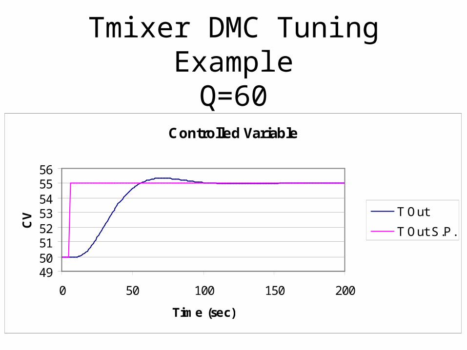
Tmixer DMC Tuning ExampleQ=60
Controlled Variable
4950515253545556
0 50 100 150 200
Time (sec)
CV T Out
T Out S.P.

Tmixer DMC Tuning ExampleQ=30
Controlled Variable
48
50
52
54
56
58
0 50 100 150 200
Time (sec)
CV T Out
T Out S.P.

Tmixer DMC Tuning ExampleQ=20
Controlled Variable
48
50
52
54
56
58
0 50 100 150 200
Time (sec)
CV T Out
T Out S.P.

Tmixer DMC Tuning ExampleQ=10
Controlled Variable
48505254565860
0 50 100 150 200
Time (sec)
CV T Out
T Out S.P.

Controller Tuning
• Reliability versus performance.
• Meeting the overall process objectives.

Checking the Controller Tuning for a Setpoint Changes in the
Opposite Direction Q=30
Controlled Variable
4445464748495051
0 50 100 150 200
Time (sec)
CV T Out
T Out S.P.

Class Exercise SISO DMC Tuning
• Tune the DMC controller for the CMixer

SISO MPC Controller
Testing

Controller Testing
• Use disturbance upsets to test controller performance

Controller Disturbance RejectionQ=60
Controlled Variable
49.5
50
50.5
51
51.5
52
0 50 100 150 200
Time (sec)
CV T Out
T Out S.P.

Controller Disturbance RejectionQ=30
Controlled Variable
49.5
50
50.5
51
51.5
52
0 50 100 150 200
Time (sec)
CV T Out
T Out S.P.

Controller Disturbance RejectionQ=10
Controlled Variable
49.5
50
50.5
51
51.5
52
0 50 100 150 200
Time (sec)
CV T Out
T Out S.P.

Class ExerciseTesting the Controller Tuning
• Using disturbance upset tests, test the performance of your tuned DMC controller.

Model Identification:The Least Squares Solution
2
1
( ) ( )
( ) is the measured value of the CV at time
( ) is the predicted value of the CV from the
SRM at time
Model ID: adjust the coefficients of
N
s i p ii
s i i
p i
i
y t y t
y t t
y t
t
the SRM
until minimized (results in averaged
SRM coeficients if enough tests are used)

Controller Disturbance Rejection Ts=7, Q=30
Controlled Variable
49.5
50
50.5
51
51.5
52
0 50 100 150 200
Time (sec)
CV T Out
T Out S.P.

What if the SRM become worse?Ts=11; Q=30
Controlled Variable
49.5
50
50.5
51
51.5
52
0 50 100 150 200
Time (sec)
CV T Out
T Out S.P.

What if the SRM become worse?Ts=15; Q=30
Controlled Variable
49.5
50
50.5
51
51.5
52
0 50 100 150 200
Time (sec)
CV T Out
T Out S.P.

SRM Model Mismatch
• The controller still works in this case, but the performance is penalized.

MIMO DMC Control

MIMO DMC Control
– Extension of SISO to MIMO
– Constraint control
– Economic LP
– Large-scale applications

MIMO DMC Control
Extension of DMC to MIMO processes

Dynamic Matrix for a MIMO Process
...
...
...
11 12 1j
21 22 2j
k1 k2 kj
A A A
A A A
.A
.
.
A A A
th
th
is the SISO
Dynamic Matrix
for the CV
and the MV
with the move
suppression factor
added
l
m
lmA

Recall The SISO Dynamic Matrix
1
2 1
3 2 1
3 3 2
3 3 3
0 0
0
Example Dynamic Matrix:
0 0
0 0
0 0
a
a a
a a a
a a a
a a a
q
q
q
A

Example of a Partitioned Dynamic Matrix
11 12
21 22
1 2 5 6
3 4 7 8
9 10 13 14
11 12 15 16
1 2 5 6
3 4 7 8
9 10 13 14
11 12 15 16
11 12
21 22
A A
A A
A AA
A A

Dynamic Matrix for a MIMO Process
...
...
...
11 12 1j
21 22 2j
k1 k2 kj
A A A
A A A
.A
.
.
A A A
th
th
is the SISO
Dynamic Matrix
for the CV
and the MV
l
m
lmA

A Partitioned Control Vector
.
.
.
1
2
j
u
u
u
u

An Example of a Partitioned Control Vector
1 3
2 4
1
2then
3
4
1 2u u
u

Control Law for MIMO DMC Controller
1[ ]
is a partitioned diagonal matrix, which
contains matrices, . is a diagonal
matrix, which contains on its diagonal.
is the relative weighting factor for
the -th CV.
i
i
w
w
i
T 2 T 2
i i
u A W A A W E
W
W W

Relative Weighting Factor
• The relative weighting factor, wi , allows the application control engineer to quantitatively rank the importance of each CV and constraint.
• For each of the constraints and CV’s, the control engineer must determine how large a violation of the constraint or deviation from setpoint requires drastic action to maintain reliable operation (Equal Concern Errors).
1
(Equal Concern Error)ii
w

Equal Concern Errors
• ECE’s are based on process experience.• Consider a distillation column
– 0.5 psi above the differential pressure limit of 2 psi will cause drastic action to prevent flooding.
– 1% impurity levels above the specified impurity levels in the products will require rerunning the product.
– Reboiler temperatures greater than 10ºF above the reboiler temperature constraint will result in excessive fouling of the reboiler.

Feedforward Variables
• Measured disturbances should be modeled as inputs for the MPC controller to reduce the effect of those disturbances on the CV.
• FF variables are treated as inputs that are not manipulated.

MIMO DMC Control
Constraint Control

Constraint Control• With DMC, constraints are treated as CV’s.• As different combinations of constraints become
active, different weighting factors, wi, are used which are based on the equal concern errors. Therefore, as different combinations of active constraints are encountered, the wi’s automatically determine the relative importance of each.
• The DMC controller determines the optimal control action based on considering that the wi’s change along the entire path to the setpoints. Therefore, the entire control law must be solved at each control interval.

MIMO DMC Control Law
1[ ]
is a partitioned diagonal matrix, which
contains matrices, . is a diagonal
matrix, which contains on itsdiagonal.
is the relative weighting factor for
the -th CV.
i
i
w
w
i
T 2 T 2
i i
u A W A A W E
W
W W

MIMO DMC Control
MPC Model Identification

MPC Model ID
2
1
( ) ( )
( ) is the measured value of the CV at time
( ) is the predicted value of the CV from the
SRM's at time
Model ID: adjust the coefficients
N
s i p ii
s i i
p i
i
y t y t
y t t
y t
t
of the SRM's
until minimized

MIMO Model Identification
• For DMC, impulse models are used for identification so that bad data can be “sliced” out of the training data.
• Sources of bad data: analyzer failure, data not recorded, process not operated in normal fashion (by-pass opened, atypical feed to the process, saturated regulatory controls, etc.), and large unmeasured disturbance to the process.

Model Identification
• SRM’s have the flexibility to model a full range of process dynamics (e.g., recycle systems).
• MPC controllers that use preset functional forms for models (e.g., state-space models or a set of preset transfer function models) can be inferior to SRM based models in certain cases.

MIMO DMC Control
Economic LP

Economic LP
• The LP combines process optimization with the DMC controller.
• The LP is based on economic parameters (e.g., product values, energy costs, etc.) and the steady-state gains of the process.
• The last term in each SRM is used to provide the necessary gain information; therefore, the LP is consistent with the MPC controller.

Example of an LP
OptimumVertex
Constraints
FeasibleRegion

Economic LP and PID Control Performance
OptimumVertex
Constraints
OperatorPID
Performance

Economic LP and MPC Control Performance
OptimumVertex
Constraints
ControlRegion
for MPC

MPC Control Performance(i.e., size of control circle)
• Depends on accuracy of models (e.g., process nonlinearity, type and size of unmeasured disturbances, changes in the process and operating conditions).
• Depends on the performance of regulatory controls and sensors.
• Can also depend on the control MPC technology used.

Economic LP
• Consider the case with 5 MV’s and 10 control objectives (i.e., upper and lower limits on CV’s, upper and lower limits on MV’s, and upper rate of change limit on MV’s): because there are 5 degrees-of-freedom (i.e., one for each MV) the LP will determine which 5 constraints to simultaneously operate against.
• The 5 constraints, in this case, become the setpoints for the MPC controller.
• The LP is applied each control interval along with the MPC controller.

The LP and the MPC Controller
• Both use the steady-state gains from the SRM.• The LP determines the setpoints for the controller
from the economic parameters and the process gains.
• The controller drives the process to the most profitable set of constraints, i.e., keeps the process making the most profit even though the most profitable set of process constraints changes with time parameters.
• Balanced ramp variables are constraints for the LP.

MIMO DMC Control
Large-Scale Applications

Size of a Typical Large MPC Application
• MV’s: 40
• CV’s: 60
• Constraints: 75-100
• There are some companies that have even larger applications.
MPC Project Organization

MPC Project Organization• Understand the process• Set the scope of the MPC controller• Choose the control configuration • Design the Plant Test• Conduct the Pretest• Conduct the Plant Test and collect the data• Analyze data and determine MPC model• Tune the controller• Commission the controller• Post audit

MPC Project Organization
Understand the process

Understand the Process
• Process understanding is the single most important issue for a successful MPC application.
• Stated another way, if you do not fully understand the process and its preferred operation, it is highly unlikely that you will be able to develop a successful MPC application.

How to Develop Process Understanding
• Study PFD’s• Study P&ID’s• Talk to the operators (how it really works!)• Talk to plant engineers (how they want it to work)• Interview plant economic planners (how much its
worth).• If available, run steady-state process simulator• Read the plant operating manuals• Spend time at the process on graveyards.

Be able to answer the following questions
• What is the purpose of the plant?
• Where does the feed come from?
• Where do the product go?
• How much flexibility is there for feed supply and product demand?
• How do the seasons affect the operation? Also, feed supply and product demand?

Be able to answer the following questions
• What are the 3 or 4 most important constraints that operators worry about?
• Where is energy used and how expensive is it?
• What are the product specifications?
• Are there environmental or tax issues that affect plant operations?
MPC Project Organization
Set the scope of the MPC controller

Set the Scope of the Project(Very Important Step)
• What part of the plant should be included in the controller? That is, how much of the plant should be included in the MPC controller to meet the project objectives?
• To answer this question, you must discuss the objectives of the project with the operations personnel, the technical staff for that portion of the plant, and the scheduling people. Only then can you be sure that you are solving the “correct” problem.

MPC Project Organization
Select the control configuration

MPC Configuration Selection
• Which PID loops do you open (i.e., turn over to MPC controller) and which do you leave closed. That is, if you leave a PID loop closed, the MPC controller sets the PID loop setpoint (e.g., flow controller).
• What are the MV’s for the distillation columns in the process? Should the MPC controller be responsible for accumulator or reboiler level control?

MPC Configuration Selection
• From an overall point of view, what are the MV’s and the CV’s for the MPC controller?
• A challenging problem that requires process knowledge and control experience while keeping focused on the overall process objectives.

Reasons for Leaving a PID Loop Closed
• The PID loop may be more effective in eliminating certain disturbance due to the higher frequency of application. For example, flow control loops. In addition, certain pressure, level, and temperature PID loops should be left closed.

Situations for which a PID loop should be opened
• Loops with very long dynamic and/or large deadtime
• Process lines with two control valves in series.• Certain levels for which allowing the MPC
controller control the level adds important flexibility to better meet the primary objectives of the process. For example, it can provide more effective decoupling.

Use Good Control Engineering
• Ensure that the MV’s have a direct and immediate affect on the CV’s.
• Use computed MV’s to reject certain disturbances, e.g., use internal reflux control to reduce the effect of rain storms or computed heat input for a pumparound.
• Use inferential measurements to reduce the effect of deadtime (e.g., inferential temp control)
• Use CV transformations that linearize the overall response of the process.

Variable Transformations
• For a control valve, P=K×Flow2
• For high purity distillation columns, use log transformed compositions: x’=log(x)
• Use different linear models depending on the operating range.

MPC Project Organization
Design the Plant Test

Plant Test Guidelines
• Make from 5 to 15 step tests for each MV• The MV changes should be as random as
possible to prevent correlated data.• MV moves should be as large as possible
but not so large that it upsets the process (e.g., 1-10%).
• For each MV, make a change after 1p, 2p, 3p, 4p, and 5p, where p is Tss/4.
• Above all, remember the product specs and the process constraints

Develop the Testing Plan
• Identify all the MV’s you plan to move. Tabulate the following data for each MV:– Tag number of the MV and physical description– Nominal value– Range of move sizes
• Make a proposed testing sequence and indicate when each MV is moved and by how much.
• Discuss the MV move sizes with operations. Remember the spec and constraints.

Choose Sampling Period
• Small sample period: high time resolution but increased size of data set. In general, sample as new information become available.
• For fast responding processes, sample every few seconds.
• For slow processes, sample every 5 min• Look at the smallest expected Tss.
– Estimate sample period as Tss/50– Compare with sensor dynamics

Make MV Changes one MV at a Time to Generate Uncorrelated Results

Develop a Roughed-out Gain Matrix
• Using your process knowledge, determine whether the steady-state process gain is positive, negative, or zero for each input (MV & DV)/ output (CV) pair.
• Using + for positive, - for negative, or 0 for zero, construct the roughed-out gain matrix. Inputs are listed vertically while outputs are listed horizontally.

Roughed-out Gain Matrix Ex.
AT
LC
LC
AT
y
L
x
S
z
PT
AT
MV's: L and SDV: zCV's: y and x

Ex. Roughed-out Gain Matrix
- ++ -+ -
L
S
y x
z
CV's
Inputs

MPC Project Organization
Conduct the Pretest

Pretest
• Check all the sensors, control valves and regulatory control loops for proper operation.
• Ensure that the process equipment is in proper repair. Check material and energy balances on the unit. Make sure that all the major pieces of equipment are in operation. Check the feed to the unit.
• Then, apply step input changes for each MV and compare to your roughed out gain matrix.
• Reconcile any deviations from what you expected (e.g., roughed out gain matrix, dynamic response, etc.). This will enhance your process understanding.

MPC Project Organization
Conduct the Plant Test and collect the data

Testing in Optimal Operating Mode
• Because you will want your plant to operate effectively at its optimum operating conditions, you should, if possible, test you plant near the optimum operating conditions to reduce the effects of process/model mismatch.
• Therefore, you will need to determine the optimum operating conditions for your plant, e.g., discuss with an experienced plant engineer or use a nonlinear process optimizer.
Plant Test Overview
• The plant test is the most important step in an MPC project because if the MPC models do not agree with the process, controller reliability and performance will be poor.
• If the process changes (e.g., different equipment configuration, different feed, different regulatory controller tuning, etc.), mismatch between the MPC model and the process will result, affecting controller performance.

Plant Test Check List
• Meet (5-10 min) with the operators at the start of each shift and explain what you are doing.
• Make sure that each MV move is made on time, in the proper direction, and by the correct amount.
• Make sure that a technical person is observing entire testing period (24-7).

Plant Test Check List
• Make real-time plots of the data and explain all the behavior that you see.
• Identify abnormal periods and make notes: significant unmeasured disturbances, instrument failures, utility outages. The MPC model should not be trained using data collected during these periods.
• Talk to the operators about the process.
• Buy pizza, donuts, ice cream and barbeque for the operators

Using Roughed-out Gain Matrix
• During the testing phase, make sure that the plant results agree with your roughed-out gain matrix.
• If not, you will need to explain the difference. That is, your process knowledge needs to be improved a bit or something is not working properly (e.g., an analyzer is off-line)

Unmeasured Disturbances
• Training an MPC controller on data collected during periods with unmeasured disturbances will reduce the accuracy of your model and reduce the effectiveness of the overall project.
• Some unmeasured disturbances are inevitable, but you must strive to keep them to an absolute minimum.

Examples of Unmeasured Disturbances to be Avoided
• Back flushing a condensor• Changes in by-pass streams• Product grade changes• Changes in the controller settings for the
regulatory controllers.• Any change in the process operating
conditions not modeled in the controller or process equipment changes

Identified Periods with Unmeasured Disturbances
• Slice out the data from those periods so that this data is not used to train the MPC model; therefore, the identified model will not be corrupted.

MPC Project Organization
Analyze the data and develop the MPC model

Obtain the MPC Process Models
• Use the accepted plant test data with the MPC model identification software to develop each of the input/output SRM models.

Evaluate Process Models
• For each input/output pair, plot the SRM on a small graph.
• Arrange the SRM models into a matrix similar to the roughed-out gain matrix.
• Review the results to ensure that you have models that make sense.
• Use the statistical tools from the MPC model ID software to evaluate each SRM

Evaluate Process Models
• Examine the difference between the plant test data and your models (residual).
• Plot the residual for positive and negative MV changes. This will help identify the degree of process nonlinearity. Also, it will help evaluate CV transformations that behave more linearly.
Plant Economics
• The LP will require incremental costs (feed costs, utility costs) and incremental revenues (product values)
• For previous distillation example, you will need the incremental cost of steam ($/lb), the incremental cost of feed ($/lb), and the incremental value of both products ($/lb).

MPC Project Organization
Tune the controller

General Approach to Tuning
• Use the SRM’s of the process (MPC model) off-line as the process to develop the preliminary settings for the controller.
• Three areas that you need to get right:– Economics– Constraints– Dynamics

Testing Economics
• Run plant/controller simulations (off-line) with different combinations of constraints to ensure that the controller pushes the plant in the correct direction.
• Run test cases to see which LP constraints are operative.

Constraints
• Check the equal concern errors for each constraint to ensure that the proper relative weighting factors for each combination of active constraints is used. That is, when constraint 1 and 5 are active, what is the relative importance of the CV’s and constraints.
• Also, use the plant/controller simulation (off-line) to test the relative weighting.

Dynamics• Select the move suppression factors for each MV
using off-line simulations of the plant. Run the simulations a number of times for setpoint changes and unmeasured disturbances to get the MSF’s right. Operators are a good source for letting you know how much the MV’s should move in certain situations and how fast the process should move to CV’s, but remember that they are most familiar with how the plant used to operate.

Operator Training
• In some states, it is a legal requirement.
• Typically operators receive one to two hours of training with MPC.
• Nevertheless, better operator training increases your chance for success.

Watchdog Timer
• The controller should run every minute 24-7
• Otherwise, a DCS alarm should sound.• The most common approach is to use a
watchdog timer (a small program running on the DCS) to communicate with the MPC controller. If the watchdog fails to receive a healthy response from the controller after an appropriate period of time, the watchdog forces each MV into a fallback (shed) position and writes an alarm to the operator.

MPC Project Organization
Commission the controller

General Approach
• Now it is time to install the controller in the closed loop in the process.
• Since the controller will directly affect the plant operation, it is essential to proceed methodically and with caution.
• Use a checklist and be observant

Commissioning Checklist
• Make sure that the operators have been trained
• Install control software, database, and other real-time components.
• Check controller database– Control CV’s, DV’s, and MV’s match raw DCS
inputs exactly– Controller models, tuning parameters, etc. match
off-line versions exactly

Commissioning Checklist (cont.)
• Turning controller on the prediction mode:– Each MV configured correctly in the DCS?– Correct shed mode for each MV?– MV’s out of cascade (controller cannot change)?– Controller turned on the prediction mode?– The size of the calculated MV moves make
sense?– The CV predictions make sense?

Commissioning Checklist (cont.)
• First-time MV check– Use conservative controller settings– Reduce difference between upper and lower
limits on MV (or rate limits)– Make sure controller is running– Put MV’s into cascade one at a time. – Ensure that the calculated MV change is
applied to DCS setpoint.

Commissioning Checklist (cont.)
• Close the loop– Ensure that the controller is running– Turn ON the controller master switch– With MV’s clamped, put one or two MV’s into
cascade– Relax the MV limits somewhat and check for
good controller behavior– Add more MV’s gradually, ensuring good control
performance.

Final Checks
• Ensure that the standard deviations of the CV’s decrease and that the MV’s are not moving around too much.
• Ensure that the LP is driving the process in the correct direction.

MPC Project Organization
Post audit

Post audit
• Collect post commissioning data for the key CV’s and compare to pre-project data.
• Ensure that the standard deviations of the key CV’s have decreased.
• Evaluate whether the upper and lower limits on the MV’s are still set correctly.
• Ensure that the controller is running the process at the economically best set of constraints most of the time.

Advantages of MPC
• Combines multivariable constraint control with process optimization.
• A generic approach that can be applied to a wide range of processes.
• Allows for more systematic controller maintenance.
• Depends on the particular process

MPC Offers the Most Significant Advantages
• For high volume processes, such as refineries and high volume chemical intermediate plants.
• For processes with unusual process dynamics.• For processes with significant economic benefit to
operated closer to optimal constraints.• For processes that have different active constraints
depending on product grade, changes in product values, summer/winter operation, or day/night operation.
• For processes that it is important to have smooth transitions to new operating targets.
Application Example
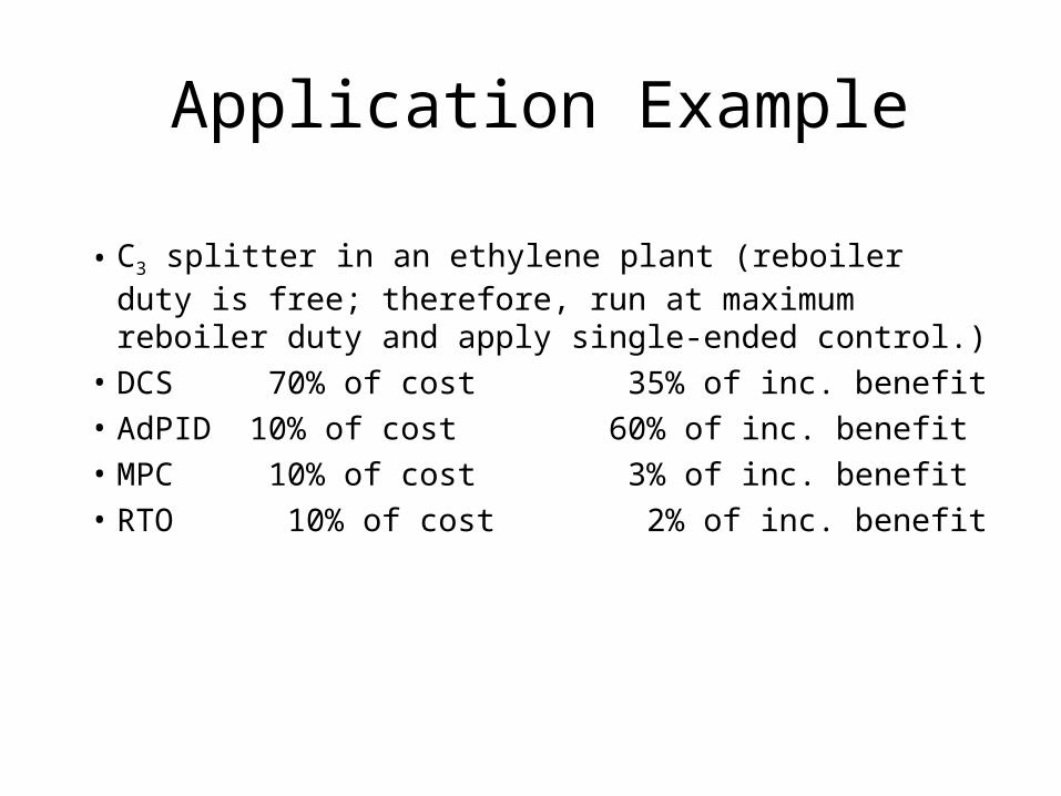
• C3 splitter in an ethylene plant (reboiler duty is free; therefore, run at maximum reboiler duty and apply single-ended control.)
• DCS 70% of cost 35% of inc. benefit
• AdPID 10% of cost 60% of inc. benefit
• MPC 10% of cost 3% of inc. benefit
• RTO 10% of cost 2% of inc. benefit

Application Example
• Reformer. Control is easy since it only involve inlet temperature controllers.
• DCS 70% of cost 35% of inc. benefit
• AdPID 10% of cost 30% of inc. benefit
• MPC 10% of cost 5% of inc. benefit
• RTO 10% of cost 30% of inc. benefit

Application Examples
• FCC Unit. Optimal constraints change with economics, operating conditions, etc. Finding the optimal riser temperature requires RTO (yield model and nonlinear problem).
• DCS 70% of cost 35% of inc. benefit• AdPID 10% of cost 10% of inc. benefit• MPC 10% of cost 35% of inc. benefit• RTO 10% of cost 30% of inc. benefit

Limitations of MPC
• It is a linear method; therefore, it is not recommended for highly nonlinear processes (e.g., pH control).
• It does not adapt to process changes. If the process changes significantly, the MPC model must be re-identified.
• For certain cases, the economic LP may not be accurate enough. For these cases, it may be necessary to add nonlinear optimization on top of the LP.

Different Forms of MPC

Primary Commercial MPC Software
• ABB
• Aspentech DMCplus
• Fisher-Rosemount
• Foxboro
• Honeywell RMPCT
• Yokogawa

• MPC software based on models with specified dynamic characteristics can be inferior to SRM based approaches.

Conclusions
Conclusions
• The challenges of this course:– A very difficult area with considerable
mathematics and industrial practice.– Only two days– Wide variety of backgrounds of the students.

Conclusions
• You should now be familiar with MPC terminology and technology and the major issues associated with the commercial application of MPC.
• Are you an MPC expert? Not yet! But with more study and a lot more experience, you can become one.

Conclusions
• “This is not the end.
• It is not even the beginning of the end.
• But it is, perhaps, the end of the beginning”
• (Sir Winston Churchill, Nov. 10, 1942)


![A data-driven Koopman model predictive control framework …predictive control framework [1], we propose a methodology for closed-loop feedback control of nonlinear ows in a fully](https://static.fdocuments.us/doc/165x107/60a0beff4add151a9d1e0f49/a-data-driven-koopman-model-predictive-control-framework-predictive-control-framework.jpg)