
Chapter 11 - ACT-Ract-r.psy.cmu.edu/wordpress/wp-content/uploads/2012/12... · Web viewChapter 11...
71
Chapter 11 Scientific Discovery Christian D. Schunn John R. Anderson Department of Psychology Carnegie Mellon University Pittsburgh, PA 15213 412-268-3499 [email protected] [email protected] In J. R. Anderson and C. Lebiere (Eds.), Atomic Components of Thought, 1998 Scientific Discovery 1
Transcript of Chapter 11 - ACT-Ract-r.psy.cmu.edu/wordpress/wp-content/uploads/2012/12... · Web viewChapter 11...
Chapter 11
Scientific Discovery
Christian D. Schunn
John R. Anderson
Department of PsychologyCarnegie Mellon University
Pittsburgh, PA 15213412-268-3499
[email protected][email protected]
In J. R. Anderson and C. Lebiere (Eds.), Atomic Components of Thought, 1998
Scientific Discovery 1

11.1 Overview
Earlier chapters have demonstrated how ACT-R can do a good job of accounting for the micro-level details of cognition. This emphasis on the micro, however, raises the question of whether ACT-R can scale to very complex cognitive tasks—can ACT-R models of very complex tasks be developed at this micro-level of detail both in a reasonable amount of time and without being overwhelmed by micro-detail? Moreover, does this micro-level of detail bring any advantages or new insights to the modeling of very complex tasks?
As an existence proof that the new ACT-R can scale to very complex tasks, we present an ACT-R model of one of the most complex task that we know of: designing and interpreting experiments in psychology. We present no proof of the relative complexity of this task, but expect that most of the readers will agree that scientific discovery is a very complex task based upon their own experiences.
In addition to providing another test of ACT-R, this chapter seeks to provide further understanding of scientific discovery behavior and expertise in general. Two particular questions will be at the center of attention. First, how much of scientific discovery behavior can be understood by examining the micro-level processes? Second, what skills underlie expertise in scientific reasoning. Addressing these questions will involve a mixture of new empirical and modeling work. But before we present this work, we will expand on this issue of expertise in scientific discovery.
There are mix of claims about the nature of scientific discovery skills. On the one hand, there are claims that it primarily involves very general skills (Qin & Simon, 1990; Shraagen, 1993; Voss, Tyler, & Yengo, 1983). For example, scientific discovery is typically thought to involve two primary activities: developing (and evaluating) hypotheses and designing experiments (cf. Klahr & Dunbar, 1988). At this basic level, it is similar to the exploratory activities of children as they interact and learn from their environment (Klahr, Dunbar, & Fay, 1993; Kuhn, 1989; Piaget, 1952) and the way many adults learn to program VCRs (i.e., by means other than reading the manual). Along those lines, some research has found that scientists do not have improved general-reasoning skills (Griggs & Ransdell, 1986; Kern, Mirels, & Hinshaw, 1983; Mahoney, & DeMonbreun, 1977). On the other hand, there are claims that it, like any other area of expertise, primarily involves many specific skills that are acquired through extended experience in the domain. For example, each scientific discipline has specific experimental paradigms (Baker & Dunbar, 1996; Kuhn, 1970; Schunn & Klahr, 1995), and specific methods for evaluating evidence (e.g., statistical tests).
To investigate the role of expertise in scientific reasoning, we conducted an experiment that attempts to empirically assess the skills available to expert and novice scientists. In the next section, we will describe this experiment and its results. Following the experiment, we will describe an ACT-R model of the task and data. Of particular importance is the issue of whether the model can further illuminate the origins and nature of expertise in a complex task like scientific reasoning.
Scientific Discovery 2

11.2 An Experimental Study of Psychological Experimentation
11.2.1 MethodThe experiment used two groups of experts (4 Domain-Experts and 6 Task-Experts) and two
groups of novices (14 High-Ability and 16 Mid-Ability undergraduates). These groups were used to tease apart the effects of domain-expertise (i.e., declarative and procedural knowledge specific to a particular domain of scientific inquiry) and the effects of task-expertise (i.e., the procedural knowledge general to scientific inquiry in many domains). The logic of the experiment was that skills for which the two groups of experts perform equally are domain-general skills, and skills for which the Domain-Experts outperform the Task-Experts are domain-specific skills (or at least require domain-specific declarative knowledge). The relative performance of the novices would testify as to whether the skills were ones learned through the experience of being a scientist or whether they were ones shared by most adults. To examine the influence of general reasoning ability, the undergraduates were divided into two groups (High-Ability and Mid-Ability1) using a median-split on Math SAT. If the differences between the undergraduates and the Task-Experts were due to task expertise and not general reasoning ability differences, then there should be no differences between the two groups of undergraduates.
We chose a particular scientific task that simultaneously satisfied three constraints: 1) the solution was unknown to the Domain-Experts, as science involves the discovery of previously-unknown solutions; 2) the problem was free of domain-specific jargon and easily understandable to even the novices; and 3) the solution was obtainable through experimentation. A problem that seemed to meet these constraints was taken from the domain of cognitive psychology. In particular, the problem was to find the cause of the spacing effect in memory—that items with longer intervening intervals tend to be better remembered.
Since the domain was memory research in cognitive psychology, the Domain-Experts were cognitive psychology faculty doing research in memory. The Task-Experts were social and developmental psychology faculty not doing research in memory. The novices were undergraduates who had not yet had courses in psychology research methods.
The subjects were given a description of the spacing effect as well as two theories about the cause of the spacing effect. These theories were simplified forms of actual theories from the literature. The first theory was the shifting-context theory, which stated that memories are associated with the context under study and that context gradually shifts with time. Under this theory, the spacing effect occurs because spaced practice produces associations to more divergent contexts which in turn are more likely to overlap with the test context. The second theory was the frequency-regularity theory, which states that the mind estimates how long memories will be needed based on regularities in the environment and, in particular, adjusts forgetting rates according to the spacing between items. Under this theory, items learned with short intervening spaces are forgotten quickly because they need not be remembered for very
1Since the novices were undergraduates were from Carnegie Mellon University, we thought it
unrepresentative to call any of them Low-Ability.
Scientific Discovery 3

long whereas items learned with long intervening spaces are forgotten more slowly because otherwise they would be long forgotten before they were needed again.
The subject’s goal was to develop experiments which could determine which explanation of the spacing effect was correct. The subjects used a computer interface called the Simulated Psychology Lab (SPL) to design experiments. The interface provided a set of variables which could be manipulated, as well as the facility to easily conduct factorial-design experiments. The use of the computer interface allowed the subjects to observe the outcomes of their experiments and iterate through several experiments—important aspects of scientific discovery.
In the interface, the subjects could manipulate six different factors: 1) repetitions—the number of times that the list of words was studied; 2) spacing—the amount of time spent between repetitions; and 3) source context—whether the studying occurred in the same context for each repetition or whether the context changed on each repetition; 4) the test task—free recall, recognition, or stem completion; 5) delay—the amount of time from the last study repetition until the test was given; and 6) test context—whether the testing occurred in the same context or a different context at test relative to the study context. For each variable, the subjects could either hold the variable constant or vary it. Values had to be selected on all dimensions, including the dimensions that were held constant in the given experiments; no default values were used. There was no restriction on the order of value selection, and subjects could go back to change their selections for any of the variables at any point in time up until they selected to run the experiment. Figure 11.1 shows the six variables that could be manipulated as they appeared on the screen and their current settings. In this example, the experiment is only partially specified, with only the repetitions and spacing variables determined—repetitions was not manipulated (it was held constant at 3) and spacing was manipulated (5 minutes vs. 20 minutes). An experiment was not complete until values for all 6 variables were specified.
Insert Figure 11.1 about here
Subjects selected variable settings by clicking on sliders and scrolling lists using a mouse. Figure 11.2 provides an example of how values were selected for the source context variable. The slider on the left was used to select whether the variable was held constant (by setting it to one—Figure 11.2a) or whether the variable was manipulated (by setting it to two or three—Figure 11.2b). Values for repetition were selected using a slider which varied from 2 to 5. Values for context and test task were selected from a scrolling list of three options. Values for spacing and delay were selected using a slider (which varied from 1 to 20) and a scrolling list of units (minutes, hours, or days).
Insert Figure 11.2 about here
The subjects made predictions and were given outcomes in a table format with all cells being shown at once. A table format was used rather than a graphical format because it was thought that the table format was less difficult to understand and manipulate for the undergraduate subjects. Before being given the table, subjects had to decide on which dimension each manipulated factor would be plotted. After deciding on the table structure, subjects made numerical predictions for their tasks. After completing their predictions, the subjects were shown the results of their experiment in table format (see Figure 11.3). In addition, the outcome
Scientific Discovery 4

tables also displayed the subject’s predictions for each cell in italics. To facilitate comparison across rows, columns, and tables, the row, column, and table marginals were also provided. To provide a rough evaluation of the quality of the predictions, the subjects were also shown the Pearson correlation between the predictions and outcomes. The actual results displayed were generated by a mathematical model that is roughly consistent with results from research on memory and the spacing effect.
Insert Figure 11.3 about here
Subjects worked at the task until they felt that they had found out what the cause of the spacing effect was. The primary data gathered in this experiment was the keystroke data generated as the subjects designed experiments, choose the table structures, and interpreted experiments. To provide additional information about the processes they used, the subjects were asked to give a think-aloud verbal protocol throughout the task, and at the end of the task they were asked to verbally report their conclusions about the two theories for the spacing effect and their conclusions about the effects of each of the six variables.
It is important to note that SPL environment and the structure of the experiment simplified many aspects of scientific discovery that a scientist would often have to accomplish. Just to name a few: the subjects did not have to work in groups (e.g., with collaborators, advisors, students, or research assistants), they did not have to propose the theories to test, they did not have to propose which variables might be manipulated, they did not have to decide on the general experimental paradigm (i.e., they were forced to use a between-subjects factorial design involving a study of words followed by a single test), there were many other variables for which values would have be selected (e.g., subject Ns) and yet were not mentioned, the subjects did not have to compute inferential statistics, and the subjects did not have to publish their results. In part, these components of scientific discovery had to be removed for practical considerations (e.g., in order to be able to present the subjects with experimental outcomes and allow them to iterate through the process of experiment design and outcome evaluation).
It is equally important to note that many of the important and difficult aspects of scientific discovery were maintained in this task. First, subjects designed experiments to test theories and evaluated those tests, two very basic and important aspects of scientific discovery. Second, the subjects were given a real scientific phenomenon, real scientific theories, and real experimental variables. In particular, the mapping of the two theories for the spacing effect onto these six variables was not simple, the typical relationship between theory and operational variables in most psychological theories and experiments. Third, there were many complex experiment design decisions that remained, as we will see in the results. Fourth, the stopping criterion for when the theories were adequately tested was not well-defined. Thus, it is fair to say that the subjects were presented with a complex and relatively ill-defined problem.2
11.2.2. ResultsComparisons of the different groups of subjects revealed several kinds of skills that were
common to experts but were lacking in undergraduates. Schunn and Anderson (1997) contains a more complete listing of skills that were examined. In this chapter we will focus on five skills that involved clear expert-novice differences. Later in the chapter we will discuss how these differences can be understood within ACT-R.
2 In fact, many of the experts complained that the task was unfairly complex.
Scientific Discovery 5
Design experiments to test the given theories. Using the verbal protocols, we classified the participants according to whether or not they mentioned either of the two theories (frequency regularity and shifting context) during the course of design experiments, either during the first experiment, or during any experiment. Note that this is a very lax criterion for measuring use of theories in experiment design—only one theory need be mentioned and the theory need only be mentioned in passing, thereby ensuring the understanding of both theories was not required to be successful under this measure. All of the Domain-Experts and Task-Experts mentioned the theories, starting with the very first experiment (see Figure 11.4). However, only 64% of the High-Ability undergraduates and 6% of the Mid-Ability undergraduates mentioned the theories during any of the experiments, significantly fewer than the Task and Domain-Experts. Thus, it appears that not even all of the brighter undergraduates understood that theories are used to guide experiment design. Instead these undergraduates simply designed experiments to explore the effects of the various factors.
Insert Figure 11.4 about here
How did these differences in orientation towards the overall task impact the choice of factors to include in the experiments? Focusing on the undergraduates, Figure 11.5 presents the proportion of undergraduates including each of the factors in their first experiment as function of whether they were trying to test theories (mentioned the theories during the design of the first experiment) or simply exploring the factors (did not mention either theory during the design of the first experiment). While the undergraduates testing theories focused on the factors relevant to the theories under test (spacing and source context), the undergraduates exploring the factors selected among the factors using a simple visual strategy, preferring leftmost and topmost variables (as shown in Figure 11.1).
Insert Figure 11.5 about here
Keep general settings constant across experiments. Another general heuristic of experimental design is to use the same constant values across experiments—it makes comparisons across experiments easier, and it capitalizes on the success of previous experiments. Note that this is subtly different than the focus of previous psychological research on variable variation (e.g., Schauble, 1990; Tschirgi, 1980). Previous research has examined whether individuals vary one factor at a time within their experiments (i.e., avoid confounding variables). In the SPL environment, the interface forces valid, factorial designs. However, there remains the issue of consistency across experiments.
Consider the following example. Suppose that in the first experiment the individual decides to vary only repetitions, selecting 2 versus 3 repetitions. The remaining variables are held constant, and the particular constant values are shown in Table 11.1. Then suppose that in the second experiment the individual decides to vary repetitions again, but this time using a stronger manipulation of 2 versus 5 repetitions. The issue of interest here is what constant values the individual selects for the other variables. They could select all the same constant values as in the first experiment (see Experiment 2 in Table 11). Alternatively, they could select different constant values (see Experiment 2’ in Table 11.1). Both permit logically valid conclusions regarding the effects of repetitions. However, Experiment 2 is more conservative; varying all
Scientific Discovery 6

the factors as in Experiment 2’ increases the risk of producing a useless experiment (e.g., producing floor or ceiling effects).
Insert Table 11.1 about here
Violations of this heuristic were counted by examining the situations in which a variable was not manipulated in consecutive experiments and then determining whether the same constant value was used in both experiments (e.g., hold spacing constant at 10 minutes across multiple experiments). Three measures of the tendency to keep values constant were used: whether the subject ever changed more than one unmanipulated variable value (i.e., minor violations), whether the subject ever changed more than two values, and whether the subject ever changed more than three values (i.e., major violations). Across the different measures of value variation, the Domain-Experts, Task-Experts and High-Ability undergraduates did not differ significantly (see Figure 11.6). By contrast, the Mid-Ability undergraduates were higher on all measures of value variation, with almost one third of them varying three or more constant values, suggesting that many of them did not understand this heuristic.
Insert Figure 11.6 about here
Avoid floor and ceiling effects. In designing experiments, it is a good heuristic to try to avoid floor and ceiling effects because they make the interpretation of null effects and interactions very problematic. To examine whether the groups were differentially effective at avoiding floor and ceiling effects, we coded which experiments produced all outcome values over 90% correct or all outcome values less than 10% correct. Figure 11.7 presents the proportion of participants with any such floor or ceiling effect experiments. The Domain-Experts never produced such experiments, indicating that domain-knowledge could be used to avoid floor and ceiling effects. The High-Ability undergraduates were just as likely as the Task-Experts to produce a floor or ceiling effect experiment, and the Mid-Ability undergraduates were even more likely to produce such an experiment—possibly a result of being less conservative in their value selections.
Insert Figure 11.7 about here
How did subjects respond to these potentially invalid experiments? Of the seven subjects producing floor or ceiling effects, five changed the delay values appropriately on the next experiment (i.e., decreasing it if there was a floor effect and increasing it if there was a ceiling effect). One subject changed the spacing values, which was also effective. The remaining subject held delays constant (at 1 minute) and, consequently, had frequent ceiling effect problems—in 6 of 9 experiments. In sum, the majority of the subjects who produced floor and ceiling effects were able to react appropriately. This combined with the previous result suggests that they understood at some level what floor or ceiling effects were and that they should be avoided, but did not initially have sufficient domain-knowledge to avoid them.
Keep experiments simple (when necessary). Another general principle of experiment design is to keep experiments simple, especially as a first approach. Figure 11.8 presents the mean experiment complexity for participants in the various groups (the mean number of factors per experiment). The Domain-Experts designed more complex experiments than did the Task-
Scientific Discovery 7

Experts, and both groups of undergraduates designed more complex experiments than did the Task-Experts. The High and Mid-Ability undergraduates produced equally complex experiments. From the verbal protocols, it was clear that the Domain-Experts were able to interpret their complex experiments, whereas the undergraduates were often overwhelmed with the large tables they produced. Thus, it appears that Domain-Experts do not need to keep experiments simple, and that undergraduates do not know that they should keep experiments simple.
Insert Figure 11.8 about here
Encode interactions and ignore noise levels. An important general outcome-interpretation skill is the ability to encode the main effects and interactions within a table. All groups of subjects were able to correctly report the main effects of the variables at the end of the task (if they had run an experiment manipulating the variables). Therefore, we can assume that the groups were all capable of encoding main effects. However, there were differences in ability to encode interactions. In this task, there were two two-way interactions. First, there was a quantitative Spacing x Delay interaction, such that the spacing effect was larger at longer delays. Second, there was an effect/no-effect Spacing x Test Task interaction, such that there was no spacing effect with stem completion. As with the main effect analysis, subjects’ final hypotheses were coded for correctness on these two interactions, and only those subjects who had conducted the relevant experiments were included in this analysis. Overall, the Domain-Experts and Task-Experts were equally able to correctly encode these interactions (see Figure 11.9). By contrast, the High-Ability undergraduates were less able to encode the interactions, and the Mid-Ability undergraduates rarely encoded the interactions.
Insert Figure 11.9 about here
In addition to being able to encode interactions when they exist, there is also the skill of noting non-interactions (i.e., not being deceived by small levels of noise). To see whether the groups differed in their ability to note non-interactions, the subjects’ final conclusions were coded for descriptions of non-existent interactions. The Domain-Experts and Task-Experts almost never made such errors, whereas the undergraduates made a significant number of such errors (see Figure 11.9). In fact, the undergraduates are just as likely to report non-existent interactions as to report existing interactions.
In sum, this experiment found several skills that are common across Domain and Task-Experts, but that many undergraduates are missing. The differences between experts and undergraduates suggests that this task tapped aspects of expertise in science. The lack of differences between Domain-Experts and Task-Experts further indicates that some aspects of this expertise are general to scientific reasoning (at least within trained psychologists). Given that bright undergraduates are missing these competencies, they must have been acquired through the practice of doing science. In the next section we present an ACT-R model of the SPL task, which may further illuminate this issue of generality of expertise.
Scientific Discovery 8
11.3 The ACT-R Model of the SPL Task
11.3.1 OverviewWe had three primary goals in building an ACT-R model of the Simulated Psychology
Laboratory (SPL) task. First, as discussed in the introduction to this chapter, we wanted to see whether we could build a model of a complex task in the new, smaller grain-sized ACT-R. Second, we were interested in what kinds of general modeling styles would emerge from building a model of this task. Many subtasks had to be solved and the methods for solving these subtasks may generalize to modeling other phenomena. Third, we were interested in what insights a detailed process model might provide for understanding the group differences observed in the SPL task. The model as presented will focus on capturing Domain-Expert performance, but we will also discuss how it can be modified to capture the group differences. We will touch upon each of these three goals throughout the description of the SPL model.
While the model is by no means a complete model of all the aspects of behavior in the SPL task, the model is quite complex, reflecting the complexity of the task. There are 48 chunk types and 116 productions. Consequently, we will overview the functionality of the model rather than simply presenting the productions.
Much of the model is concerned with interactions with the environment. That is, at many points the model has to encode information from the visual array or perform actions in that array. While we could, we have not made the model interact with the actual SPL interface (because it would have to be re-implemented in LISP). Nonetheless, we were careful to put into the model the necessary rules for interacting with the interface. Most importantly, the model distinguishes between internal and external memory, and productions do not directly access external memory. Thus, the model could be hooked up to a LISP re-implementation of the interface without having to modify the core productions. The details of these rules will be discussed relatively little in this report, but they can be examined in the actual model on the Web.
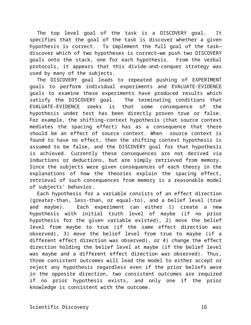
The top level goal of the task is a DISCOVERY goal. It specifies that the goal of the task is discover whether a given hypothesis is correct. To implement the full goal of the task—discover which of two hypotheses is correct—we push two DISCOVERY goals onto the stack, one for each hypothesis. From the verbal protocols, it appears that this divide-and-conquer strategy was used by many of the subjects.
The DISCOVERY goal leads to repeated pushing of EXPERIMENT goals to perform individual experiments and EVALUATE-EVIDENCE goals to examine these experiments have produced results which satisfy the DISCOVERY goal. The terminating conditions that EVALUATE-EVIDENCE seeks is that some consequence of the hypothesis under test has been directly proven true or false. For example, the shifting-context hypothesis (that source context mediates the spacing effect) has as a consequence that there should be an effect of source context. When source context is found to have no effect, then the shifting context hypothesis is assumed to be false, and the DISCOVERY goal for that hypothesis is achieved. Currently these consequences are not derived via inductions or deductions, but are simply retrieved from memory. Since the subjects were given consequences of each theory in the explanations of how the theories explain the spacing effect, retrieval of such consequences from memory is a reasonable model of subjects’ behavior.
Each hypothesis for a variable consists of an effect direction (greater-than, less-than, or equal-to), and a belief level (true and maybe). Each experiment can either 1) create a new
Scientific Discovery 9
Christian Schunn, 01/03/-1,
4 motor productions, 62 regular productions, 29 table productions, 21 visual productions

hypothesis with initial truth level of maybe (if no prior hypothesis for the given variable existed), 2) move the belief level from maybe to true (if the same effect direction was observed), 3) move the belief level from true to maybe (if a different effect direction was observed), or 4) change the effect direction holding the belief level at maybe (if the belief level was maybe and a different effect direction was observed). Thus, three consistent outcomes will lead the model to either accept or reject any hypothesis regardless even if the prior beliefs were in the opposite direction, two consistent outcomes are required if no prior hypothesis exists, and only one if the prior knowledge is consistent with the outcome.
Each EXPERIMENT goal leads to the design, running, and encoding of one experiment (see Figure 11.10). There are three different subtypes of EXPERIMENT goal which can be thought of as different experimental paradigms: HYPOTHESIS-TESTING, EXPLORE-SYSTEM, and TEST-FACTOR.3 The HYPOTHESIS-TESTING and EXPLORE-SYSTEM subtypes correspond to the two general approaches that subjects took towards the task: designing experiments relevant to the hypotheses versus simply investigating the effects of the six factors. Previous models of scientific discovery have also distinguished among such different approaches to experimentation (e.g., Cheng, 1990; Klahr & Dunbar, 1988; Shrager, 1985, 1987). The TEST-FACTOR is produced as a consequence of an experiment which produced an ambiguous result that needs to be explored further. The three types of goals lead to similar experiment design behaviors although there are some critical differences. In the next subsection, we will first describe experimental design for hypothesis testing. Then we will discuss the differences for the other two types of goals.
Insert Figure 11.10 about here
11.3.2 Experimental DesignThe experimental design process is similar for the three EXPERIMENT goal subtypes in
Figure 11.10. We will describe the experimental design process with respect to the HYPOTHESIS-TESTING goal. A HYPOTHESIS-TESTING goal produces the overall structure of designing an experiment to test a hypothesis. A HYPOTHESIS-TESTING goal pushes two primary goals: to vary the hypothesis factors and to fix the remaining variables. The goal to vary hypothesis factors selects whether to vary one or two factors relating to the hypothesis and which factors to vary. The goal to fix the remaining variables then iterates over the variables visually and selects the remaining unselected variables.
The content of the hypothesis under test drives the selection of factors to vary. The hypothesis has three components: the variable causing the effect, the direction of the effect of the variable (greater-than, less-than, equal-to), and the current belief level (true or maybe). To select a variable to manipulate, the simulation searches for a consequence of the hypothesis under test, which names a variable and an expected effect direction. For example, a consequence of the shifting-context theory is that source-context should have a greater-than effect (i.e., varying study contexts should improve retention). The simulation then sets a goal to vary that consequent variable.
A series of productions are responsible for setting the factors. They start with task-specific productions of the form “if you want to vary some factor and you are looking at the main screen then press the button relating to that factor”. When the screen relating to the desired factor is achieved, a VARIABLE-SETTING goal is created and pushed on the stack. This VARIABLE-
3 Note that these different types of experiment goal, not subgoals of the experiment goal.
Scientific Discovery 10

SETTING goal serves as both a control structure and a memory for details of the experiment design. The VARIABLE-SETTING goal initially contains only information about which variable is being considered. Incrementally, slots are filled regarding the number of levels of that variable and what value each level has. For example, if the repetitions variable is to be varied, then the number of levels is set at two, value1 may be set to three, and value2 may be set to five. Alternatively, if the repetitions variable is not to be varied, then the number of levels is set at one, value1 may be set to three repetitions, and value2 is left empty.
By default, if the simulation does not have a goal to vary this particular factor, it chooses not to vary the factor. However, there is one exception. If the simulation is planning on varying some other factor B and can retrieve an INTERACTION hypothesis involving that factor and the current factor A, then the simulation chooses to vary the current factor. In other words, the simulation prefers to vary only the one selected factor unless it expects to find interactions with that factor. More will be said about these INTERACTION hypotheses when it comes to encoding the results of experiments.
How are particular values selected for each variable? Knowledge of possible selections for a particular variable are presented in the form of POSSIBLE-SELECTION chunks. At first, when the simulation has not previously considered a variable, it has no POSSIBLE-SELECTION chunks in memory for that variable, and must create POSSIBLE-SELECTIONS by conducting a visual search of the options available in the interface. This visual search creates a POSSIBLE-SELECTION chunk for each possibility. Given a set of POSSIBLE-SELECTION chunks, there are four alternative schemes for selecting a particular one. The alternative schemes are implemented as productions competing in conflict resolution. The first scheme is to choose the visually leftmost (or topmost) selection. The second scheme is to choose randomly among the POSSIBLE-SELECTIONS, which favors the most active one in memory. The third scheme is to specifically retrieve the value that was used for that variable in a prior experiment (and activation differences will favor the just previous experiment). The fourth and final scheme is to retrieve specific knowledge of what values must be avoided and find a value that satisfies these constraints. For example, a previous experiment may have determined that short delay values lead to ceiling effect problems. Therefore, short delay values will be avoided.
The alternative EXPERIMENT goal types in Figure 11.10 have similar goal structures as the HYPOTHESIS-TESTING goal. The most similar is TEST-FACTOR, which pushes a goal to vary the factor it desires to test and another goal to fix the remaining variables. In contrast, EXPLORE-SYSTEM simply conducts a visual search for the variables not yet set, and then pushes a goal to vary the first such factor found.
11.3.3. Encoding the TableAfter the experiment is designed and run, the resulting table must be encoded. The
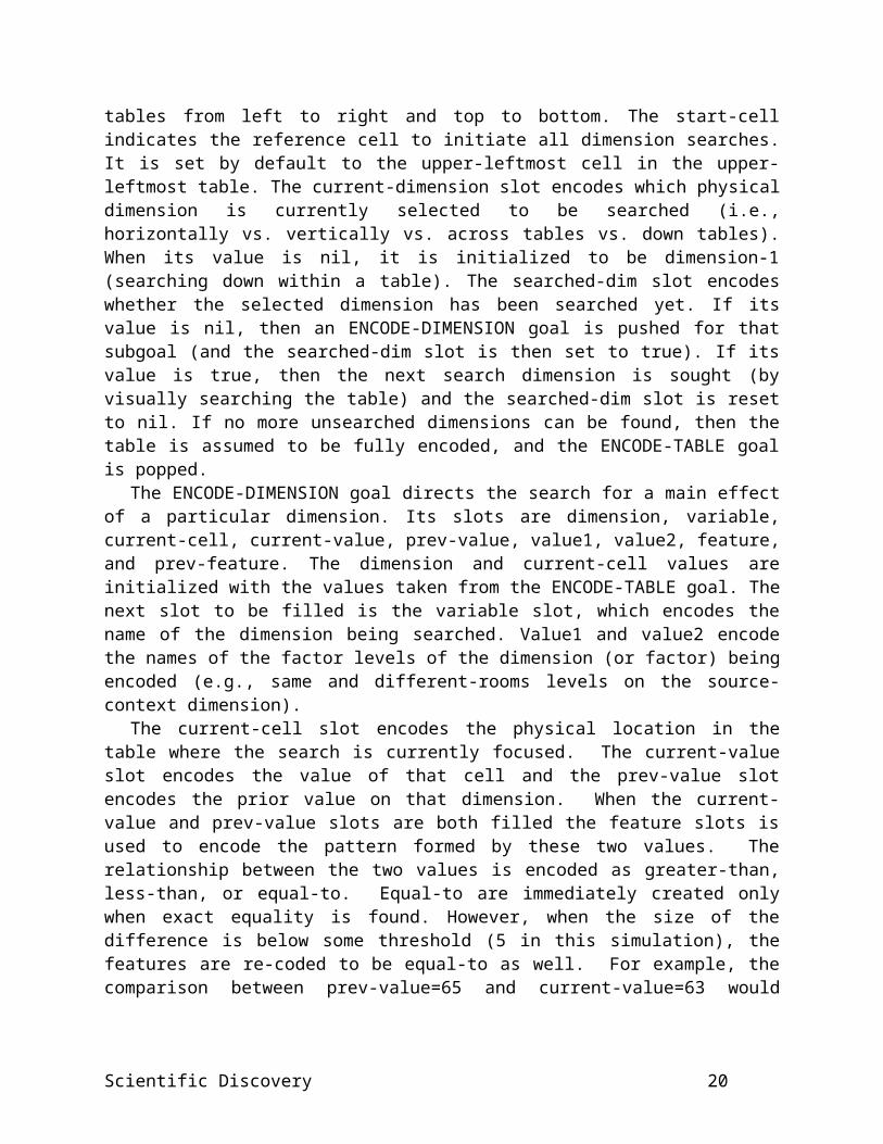
ENCODE-TABLE goal initializes and directs the search over the table, setting ENCODE-DIMENSION subgoals for each of the table dimensions. The slots of ENCODE-TABLE are method, start-cell, and current-dimension, and searched-dim. All of these slots start out empty and are filled in that order. The method slot encodes the method that will be used to search the table. The LtR-scan method is the default method and searches tables from left to right and top to bottom. The start-cell indicates the reference cell to initiate all dimension searches. It is set by default to the upper-leftmost cell in the upper-leftmost table. The current-dimension slot encodes which physical dimension is currently selected to be searched (i.e., horizontally vs. vertically vs. across tables vs. down tables). When its value is nil, it is initialized to be dimension-1 (searching down within a table). The searched-dim slot encodes whether the selected dimension has been searched yet. If its value is nil, then an ENCODE-DIMENSION goal is pushed for that subgoal
Scientific Discovery 11

(and the searched-dim slot is then set to true). If its value is true, then the next search dimension is sought (by visually searching the table) and the searched-dim slot is reset to nil. If no more unsearched dimensions can be found, then the table is assumed to be fully encoded, and the ENCODE-TABLE goal is popped.
The ENCODE-DIMENSION goal directs the search for a main effect of a particular dimension. Its slots are dimension, variable, current-cell, current-value, prev-value, value1, value2, feature, and prev-feature. The dimension and current-cell values are initialized with the values taken from the ENCODE-TABLE goal. The next slot to be filled is the variable slot, which encodes the name of the dimension being searched. Value1 and value2 encode the names of the factor levels of the dimension (or factor) being encoded (e.g., same and different-rooms levels on the source-context dimension).
The current-cell slot encodes the physical location in the table where the search is currently focused. The current-value slot encodes the value of that cell and the prev-value slot encodes the prior value on that dimension. When the current-value and prev-value slots are both filled the feature slots is used to encode the pattern formed by these two values. The relationship between the two values is encoded as greater-than, less-than, or equal-to. Equal-to are immediately created only when exact equality is found. However, when the size of the difference is below some threshold (5 in this simulation), the features are re-coded to be equal-to as well. For example, the comparison between prev-value=65 and current-value=63 would result in an equal-to feature (after first encoding a less-than feature).
Once the feature is encoded, the search for effects of that dimension continues in the next row (or column) of the table. For example, in a 2x2 table, the first column is searched first, followed by the second column. When the search of the second column begins, the value of the feature slot is placed in the prev-feature slot, and the feature slot is reset to nil. At the end of the search of the second column (and all subsequent ones) of a given dimension, the values of the feature and prev-feature slot are compared. If the two values are the same, then the search continues. When there are no new columns to search, the simulation assumes there is a consistent main effect of the dimension and the ENCODE-DIMENSION goal is popped. When the two values are not the same, then the simulation assumes there is an interaction and no consistent main effect and the ENCODE-DIMENSION goal is popped even if there are more columns to encode on that dimension.
In either case (consistent or no consistent main effect), a TEST-GENERALITY goal is pushed, with the name of the examined variable and the found feature, in the consistent case, or with an equal-to feature, in the inconsistent case. The generality of the feature is tested by comparing it to the current hypothesis regarding that variable. If no such hypothesis exists, it is created and the truth level is set to maybe. If the hypothesis for that variable exists and is consistent with current outcome, then the hypothesis truth level is strengthened (i.e., is changed from maybe to true). However, if the hypothesis is inconsistent with the current outcome, then a subgoal to explain the inconsistency is pushed.
The subgoal to explain the inconsistency initiates a search for possible design problems in the current experiment that might have lead to misleading results. The simulation can currently detect three types of problems. If the values in the table are above 90% and there was no effect of the variable, then the simulation proposes that there was a ceiling effect. If the values in the table are below 10% and there was no effect of the variable, then the simulation proposes that there was a floor effect. If the two values of the variable were too close together (e.g., one minute and two minutes) and there was no effect, then the simulation proposes that the manipulation was too weak. In the case of the floor and the ceiling effects, the simulation examines the details of the experiment design to see what might have caused those effects.
Scientific Discovery 12

A discovered experiment problem is stored in a chunk (called EXPERIMENT-PROBLEM) which then can be used to influence later experiment designs. In the case of a weak manipulation, the next experiment will use the TEST-FACTOR paradigm to design the experiment (instead of TEST-HYPOTHESIS or EXPLORE-SYSTEM). For all three types of problems, when that particular variable is being considered during the design of the next experiment, a production will set a subgoal to try to find a value which avoids the problematic values found in the previous experiment. Thus, while the simulation is conservative in that it prefers to pick the same variable values as in the previous experiment, it will specifically avoid values that were found to be problematic.
When interactions are found, an INTERACTION chunk is created an pushed as a goal. Its slots are variable1, variable2, feature1, feature2, cell, and prev-cell. Variable1 encodes the variable that was being searched when the interaction was found. Feature1 and feature2 encode the two inconsistent features that were found. Cell encodes the table location that was last viewed when the interaction was found (and was associated with feature2). To determine what the interacting variable (variable2) was, the simulation first retrieves a cell that was associated with the other feature (feature1), and then determines which dimension differentiated the two cells.
In sum, experiments are designed by considering factors one at a time, focusing on the theory-relevant ones first. Experiment outcomes are interpreted by scanning the table, noticing main effects and interactions, and testing the generality of these effects. The simulation iterates through these processes until the hypothesis under test has been either confirmed or disconfirmed.
11.3.4 General features of the modelThere were a number of general approaches adopted in this model which are useful in
developing ACT-R models for many domains. We will mention three here. Performance in this task required interleaving productions that were not specific to the interface with productions that were (cf. Gray, 1997). For instance, experimentation-general productions selected which variables were relevant to the hypothesis but device-specific productions chose to initiate manipulation of the variable by pressing the button for that variable. The experimentation-general productions represent what subjects knew about designing experiments before our task whereas the device-specific productions represent what they had to learn to perform our task. The critical problem is to enable the general productions to transfer from scientific discovery to our task without having the specific productions learned in our task transfer back to other environments. For example, our expert subjects would not want to return to their offices, try to design an experiment, and then be looking for a particular factor button on the screen. This delimitation of transfer was achieved by giving all goals a looking-at slot which referred to the general contents of the current screen. The device-specific productions contained tests for the value of the slot and so would not generalize to other contexts.
Second, we used a context slot to bind together in memory all the chunks representing a particular experiment. For example, there were VARIABLE-SETTING chunks encoding the values selected for each factor and ENCODE-DIMENSION chunks encoding the outcomes for each variable that was varied. The model could tell when they referred to the same experiment by seeing if they had the same value in the context slot. This allows the model to distinguish between the current experiment and previous experiments, all of which must be maintained in declarative memory. This use of the context slot is similar to the list slot used in the simulations of the list memory experiments (see Chapter 7) and is an idea that can be traced back to the list memory models of Anderson and Bower (1972). In the SPL simulation, the context slot is
Scientific Discovery 13

always the number of the current experiment. This context value is automatically updated when a new experiment is begun.
A third feature of the simulation is the distinction between memory retrieval and visual retrieval. In many instances, information can be obtained either by doing a memory retrieval or by setting a VISUAL-SEARCH goal to retrieve the information from the interface. For example, in the design of experiments after the first one, the POSSIBLE-SELECTION chunks can either be retrieved from memory from the design of the previous experiment, or new ones can be created again by another visual search of the interface. With production parameter learning turned on, the productions tune themselves to switch from visual retrieval to memory retrieval over time.
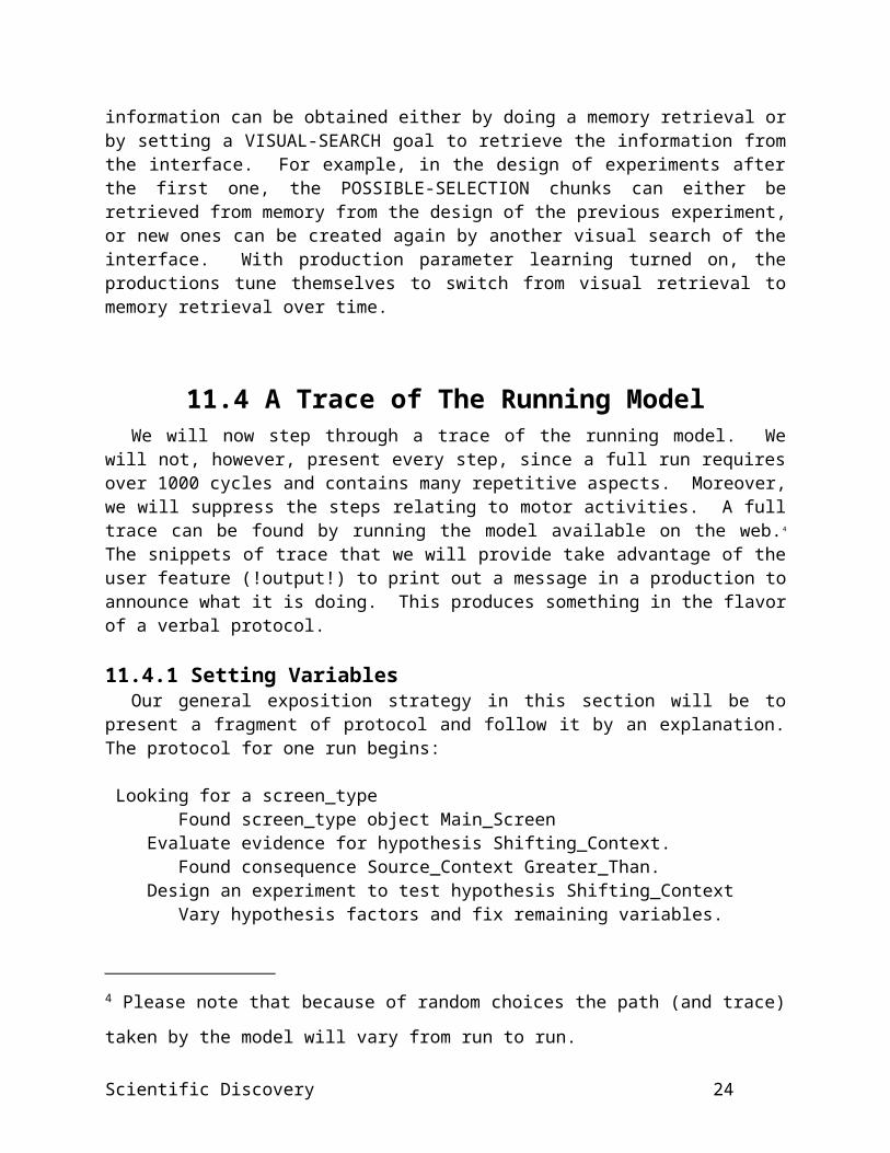
11.4 A Trace of The Running ModelWe will now step through a trace of the running model. We will not, however, present every
step, since a full run requires over 1000 cycles and contains many repetitive aspects. Moreover, we will suppress the steps relating to motor activities. A full trace can be found by running the model available on the web.4 The snippets of trace that we will provide take advantage of the user feature (!output!) to print out a message in a production to announce what it is doing. This produces something in the flavor of a verbal protocol.
11.4.1 Setting VariablesOur general exposition strategy in this section will be to present a fragment of protocol and
follow it by an explanation. The protocol for one run begins:
Looking for a screen_type Found screen_type object Main_Screen Evaluate evidence for hypothesis Shifting_Context. Found consequence Source_Context Greater_Than. Design an experiment to test hypothesis Shifting_Context Vary hypothesis factors and fix remaining variables. Found consequent variable Source_Context of the hypothesis Shifting_Context Vary variable Source_Context Click on the button relating to factor Source_ContextACTION: Click button 3LEFTNEW SCREEN: Choose Variable
The model begins by looking to environment to uncover what screen_type is on the screen and finds that the environment is in the MAIN_SCREEN state. Then the model evaluates the current evidence for the hypothesis under test by considering when one of its consequences is true. It cannot retrieve an knowledge about the truth of this consequence and so returns to designing an experiment. At this point, the model chooses to design an experiment to test the shifting-context hypothesis (i.e., push the HYPOTHESIS-TESTING subgoal). This in turn
4 Please note that because of random choices the path (and trace) taken by the model will vary
from run to run.
Scientific Discovery 14
pushes goals to vary factors relevant to the hypothesis and fix the remaining factors. With respect to varying factors relevant to the hypothesis, the model selects to vary the variable identified in one of the consequences of the hypothesis. The model then clicks on the button relating to that factor.5 The protocol continues:
Looking for a screen_type Found screen_type object Source_Context On the right screen to pick Source_Context How many levels are we currently at for Source_Context? Found nlevels One Source_Context is at 1, but we want 2, so change it Clicking slider Source_ContextACTION: Update nlevels for Source_Context to Two Look for options for variable Source_Context Visually found option Same Visually found option Diff_Room Visually found option Diff_Mood Pick the top value (Same) as a default. Making selection One for Source_ContextACTION: Update value One for Source_Context to be Same Picking Diff_Room as second value. Making selection Two for Source_ContextACTION: Update value Two for Source_Context to be Diff_Room Done picking values for Source_ContextACTION: Click Done NEW SCREEN: Main Screen
After clicking on the source-context button, the model discovers that it is now on the correct screen to actually modify source-context. It then creates a VARIABLE-SETTING goal for source-context and proceeds to fill in the slots for that goal. The first slot to be filled is how many levels is the variable currently set at, which it discovers is currently at one. However, since the goal was to vary this variable, this must be updated to two. Then the model looks to the environment to discover which possible selections there are. Three are found (Same, Diff-Room, and Diff-Mood), and Same is selected for the first value (because it the topmost value in the interface), and Diff-Room is selected randomly for the second value (since it happened to be the most active in memory, other than Same). Thus, this aspect of the experiment is designed without significant amounts of knowledge. The protocol continues:
Looking for a screen_type Found screen_type object Main_Screen Look for first unselected variable.
5As a note about the trace formatting: When the model takes a physical action, the lisp code
implementing this action states which action was taken (ACTION: ) and what new screen is
displayed if there is a screen change (NEW SCREEN: ).
Scientific Discovery 15
Found variable Repetitions Consider factor Repetitions Click on the button relating to factor RepetitionsACTION: Click button 1LEFTNEW SCREEN: Choose Variable Looking for a screen_type Found screen_type object Repetitions On the right screen to pick Repetitions How many levels are we currently at for Repetitions? Found nlevels One Search memory to see if Source_Context is an interacting variable with Repetitions Look for options for variable Repetitions Visually found option Two Visually found option Three Visually found option Four Pick the top value (Two) as a default. Making selection One for RepetitionsACTION: Update value One for Repetitions to be Two Done picking values for RepetitionsACTION: Click Done NEW SCREEN: Main Screen...
Back at the MAIN_SCREEN, the model looks for the nextmost unselected variable and finds repetitions. For this variable, the number of levels is left unmodified at one as a default, and the topmost value of two is selected as the value. This process continues until values for the remaining four variables are selected.
11.4.2 Interpreting an ExperimentWe resume the protocol when the experiment design is complete:...Looking for a screen_type Found screen_type object Main_Screen Look for first unselected variable. Finished selecting variable values. Finished designing the experiment, click on runACTION: Click Run NEW SCREEN: Outcome TableExper1 Repetitions --- Two Spacing --- One_minute Source_context --- Same Diff_room Test_task --- Stem Delay --- One_minute Test_context --- SameSource_ContextSame 100Diff_Room 99
Scientific Discovery 16

When no more unselected variables can be found, the experiment design is complete and the experiment is run. The simulation of the SPL task prints the designed experiment and outcome of the experiment. In this case, only source-context was varied, and the results were 100% for Same and 99% for Diff-room. Below the interpretation of these results begins:
Looking for a screen_type Found screen_type object Outcome_Table Encode table. Try scanning left-to-right. Visually find starting place--top left. Found top-left cell 1111 Start with dimension dim1. Push goal to encode dimension Dim1 Visually get cell value Found value 100 Look for value1 visually Found dimension value Same Visually locate dimension variable. Found dimension name Source_Context
To encode the outcomes, the model first selects the default scanning strategy—top-down, left-to-right. Then the model locates the table reference cell (upper-leftmost—encoded as 1111) to begin the search. Finally, the model looks for a dimension to search, beginning with dimension1 (going down). Since this dimension has not yet been searched (i.e., no ENCODE-DIMENSION chunk for that dimension can be retrieved), the model pushes an ENCODE-DIMENSION goal to search that dimension. At this point, the model could either look to find the name of dimension variable, or encode the contents of the first cell. In this case, it happens to encode the contents of the first cell (100 percent). Then it searches for the value on that dimension that corresponds to the cell (Same). Finally, it looks for the name of the dimension variable (Source Context).
Move in desired direction. Found location below, 2111 Visually get cell value Found value 99 Look for value2 visually Found dimension value Diff_Room Notice less than pattern. Difference -1 in Dim1 is not significant. Finished first row of dimension Dim1.
The model then moves to the next cell in the direction of the search dimension, encodes the cell contents, and discovers what variable value is associated with that cell (Diff-room). Comparing the table cell values of 99 and 100 (encoded in the earlier trace fragment), the model creates a pattern chunk encoding a less-than relation. This feature is elaborated to note that the difference of 1 is not significant, thereby changing the feature to an equal-to relation. Then the
Scientific Discovery 17

first pass at dimension 1 is complete, and the model attempts to move to the next row (or column in this case) in this dimension.
Finished encoding dimension. See if main effect generalizes. Hypothesize that Source_Context may have no effect and check for problems. Pop hypothesis. Rehearsing hypothesis involving Source_Context Suspect a ceiling effect. Delay One_Minute too short. Rehearsing experiment_problem involving Delay...
Since there are no more rows to search on that dimension, and no interactions have been found, the model assumes that the found effect (equal-to) is the main effect for that dimension and tests the generality of that effect. No previous hypotheses for that variable are found, and so a new hypothesis is proposed that it may not produce an effect. This hypothesis is also rehearsed once to insure that it will be remembered later. Since there was no effect of the variable, the model also looks for problems in the experiment that might have lead to an artifactual null result. Since the values were above 90%, the model suspects a ceiling effect, and guesses that the delay of One-minute was too short. This proposed experiment-problem is also rehearsed once to insure that it will be remembered during the design of the next experiment.
11.4.3 Designing a Second ExperimentThe critical portion of the design of the second experiment begins:
... Evaluate evidence for hypothesis Shifting_Context. Found consequence Source_Context Greater_Than. Design an experiment to test hypothesis Shifting_Context Vary hypothesis factors and fix remaining variables. Found consequent variable Source_Context of the hypothesis Shifting_Context Vary variable Source_ContextACTION: Click button 3LEFTNEW SCREEN: Choose Variable
Again, the model evaluates the evidence for the hypothesis under test, and finds no definite evidence for or against. For the next experiment, the model chooses again to vary source-context because it is involved in a consequence of the shifting-context theory.
Looking for a screen_type Found screen_type object Source_Context On the right screen to pick Source_Context Already know options for Source_Context How many levels are we currently at for Source_Context? Found nlevels One
Scientific Discovery 18

Source_Context is at 1, but we want 2, so change itACTION: Update nlevels for Source_Context to Two Pick previous value Same. Making selection One for Source_ContextACTION: Update value One for Source_Context to be Same Picking previous value2 (Diff_Room) Making selection Two for Source_ContextACTION: Update value Two for Source_Context to be Diff_Room Done picking values for Source_ContextACTION: Click Done NEW SCREEN: Main Screen...
Since this is no longer the first experiment to be designed, the process is changed. Since the model can remember the possible options presented previously, it no longer has to look externally to find these options. Moreover, instead of choosing values arbitrarily, the model specifically chooses the same first value for source-context as in the previous experiment. Although it is not shown, the process for picking the other variables is similarly shortened. We will, however, look at the critical selection of the delay variable:
... On the right screen to pick Delay Already know options for Delay How many levels are we currently at for Delay? Found nlevels One Look for something greater than One_Minute Failed finding something for value1. Look for more options. Visually found option One_Minute Visually found option Five_Minutes Visually found option Ten_Minutes Look for something greater than One_Minute Found Ten_Minutes to be greater than One_Minute Making selection One for DelayACTION: Update value One for Delay to be Ten_Minutes...Exper2 Repetitions --- Two Spacing --- One_minute Source_context --- Same Diff_room Test_task --- Stem Delay --- Ten_minutes Test_context --- SameSource_ContextSame 64Diff_Room 64...
Scientific Discovery 19
The process of selecting a value for the delay variable is changed in one additional manner. Because there was an experiment problem associated with delay in a previous experiment, the model explicitly sets a goal of avoiding this problematic value (one-minute). However, the model forgot about values other than one minute, and must do another visual search of the available options. Then, a delay of ten-minutes is selected instead of the previously selected one-minute delay. Consequently, the resulting experiment no longer suffers from ceiling effects. The search process through the table, not shown above, is the same as in the previous experiment. Once again, the model finds no effect of source context, and therefore concludes that it definitely has no effect:
... Evaluate evidence for hypothesis Shifting_Context. Found consequence Source_Context Greater_Than. Found consequence to be false. Therefore reject hypothesis Shifting_Context. Examined consequence. Therefore done testing hypothesis Shifting_Context.
When the evidence is evaluated again, the shifting-context hypothesis is rejected because its consequence involving source-context is found to be false. The model then turns to examining the frequency regularity hypothesis.
11.4.4 Testing the Frequency Regularity Theory
The design of the third experiment begins:
Update context for Start2 to be Exper3 Looking for a screen_type Found screen_type object Main_Screen Evaluate evidence for hypothesis Frequency_Regularity. Found consequence Spacing Greater_Than. Design an experiment to test hypothesis Frequency_Regularity Vary hypothesis factors and fix remaining variables. Found consequent variable Spacing of the hypothesis Frequency_Regularity Vary variable Spacing...
The model decides to vary spacing, a variable implicated in a consequence. The critical portion of the variable selection is reproduced below:
... On the right screen to pick Spacing How many levels are we currently at for Spacing? Found nlevels One Spacing is at 1, but we want 2, so change itACTION: Update nlevels for Spacing to Two Already know options for Spacing Pick previous value One_Minute.
Scientific Discovery 20

Making selection One for SpacingACTION: Update value One for Spacing to be One_Minute Failed finding something for value2 in memory. Look for more options. Visually found option One_Minute Visually found option Five_Minutes Visually found option Ten_Minutes Picking Five_Minutes as second value. Making selection Two for SpacingACTION: Update value Two for Spacing to be Five_Minutes Done picking values for SpacingACTION: Click Done NEW SCREEN: Main Screen...
In selecting values for spacing, the simulation chooses the same first value from the previous experiments. However, in selected the second value, it must re-examine its options visually because it has forgotten what the other options were. Five minutes is selected as the second value (because it happens to be most active in memory). The model selects the other values as before, but when it comes to selecting test task something interesting happens:
... On the right screen to pick Test_Task Already know options for Test_Task How many levels are we currently at for Test_Task? Found nlevels One Search memory to see if Spacing is an interacting variable with Test_Task Found interaction between Spacing and Test_Task. Test_Task is an interacting variable with Spacing, so set nlevels to 2ACTION: Update nlevels for Test_Task to Two Pick previous value Stem. Making selection One for Test_TaskACTION: Update value One for Test_Task to be Stem Failed finding something for value2 in memory. Look for more options. Visually found option Recall Visually found option Recog Visually found option Stem Picking Recall as second value. Making selection Two for Test_TaskACTION: Update value Two for Test_Task to be Recall Done picking values for Test_TaskACTION: Click Done NEW SCREEN: Main Screen...
When it examines test task, it find the prior belief that test task may interact with the spacing variable. This reflects the sort of knowledge we might expect of a memory expert. Also, when it comes to the variables of delay, it retrieves the fact that the frequency regularity theory implies
Scientific Discovery 21

an interaction of spacing and delay. Therefore it chooses to vary that, too (this decision is not shown in the protocol). The experiment finally designed is shown below:
...NEW SCREEN: Outcome TableExper3 Repetitions --- Two Spacing --- One_minute Five_minutes Source_context --- Same Test_task --- Stem Recall Delay --- Ten_minutes One_minute Test_context --- SameDelay Ten_Minutes Test_Task Spacing Stem Recall One_Minute 65 11 Five_Minutes 63 31 One_Minute Test_Task Spacing Stem Recall One_Minute 100 93 Five_Minutes 99 92...
Experiment 3 results in a three-dimensional table, whose results show the interaction of spacing with test-task.
11.4.5 Interpreting an InteractionThe interpretation of this table is interesting because it contains an interaction.
... Start with dimension dim1. Push goal to encode dimension Dim1 Visually get cell value Found value 65 Visually locate dimension variable. Found dimension name Spacing Look for value1 visually Found dimension value One_Minute Move in desired direction. Found location below, 2111 Visually get cell value Found value 63 Look for value2 visually Found dimension value Five_Minutes Notice less than pattern. Difference -2 in Dim1 is not significant. Finished first row of dimension Dim1.
Scientific Discovery 22

The model begins with the first dimension as before, encodes the first column, and finds an equal-to relation. Then it searches the second column:
Visually get cell value Found value 11 Move in desired direction. Found location below, 2211 Visually get cell value Found value 31 Notice greater than pattern. Found interaction. No main effect? Investigate interaction. Found the cell 2111 with the Equal_To effect. Search for variable which separates 2211 from 2111. Found separating dimension, Test_Task Done investigating interaction of Spacing with Test_Task.
This time, however, the search over that dimension is not finished. The next column is searched, and a greater-than relation is found. Note that the dimension name and dimension values must only be examined for the first column that is searched—that information is simply carried over for the other columns. Since the greater-than effect is different than the equal-to effect found in the first column, the model assumes no main effect and investigates this interaction. This involves looking for the cell that produced the other effect (equal-to), and then searching for the dimension that separates that cell from the current one. The resulting dimension (test-task) is assumed to interact with the current one (spacing).
Hypothesize that Spacing may have no effect and check for problems. Pop hypothesis. Rehearsing hypothesis involving Spacing Insufficient range One_Minute Five_Minutes Rehearsing hypothesis related to Spacing Rehearsing experiment_problem involving Spacing...
Since an interaction was found, the search of that dimension halts and the variable (spacing) is assumed to have no main effect. The generality of this relationship is tested. Since there are no priors for this variable, the model tentatively assumes there may be no effect of spacing and checks for possible experiment problems which may have produced an artificial null result. It suspects that the difference of one-minute versus five-minutes (in the spacing manipulation) may have been an insufficient range. The hypothesis for spacing and this experiment problem is rehearsed to insure that it will be remembered later.
Note that the model’s reasoning about the absence of a main effect is not the same as what would be produced by an ANOVA. Even though there may be an effect of spacing overall, the model reasons (as did the Domain-Experts) that because there is a case in which there is no spacing effect, then the prediction of a consistent main effect of spacing is falsified (and hence the Frequency Regularity is falsified). In general, the model reasons about main effects and interactions qualitatively rather than quantitatively. In fact, purely quantitative interactions (same effect direction but different magnitudes) are ignored.
Scientific Discovery 23
The rest of the examination of the table is not shown but we will briefly summarize it. Since there is a second dimension (and it has not yet been searched), the model turns to this second dimension (going across within a table). The values 65 and 11 are encoded, along with the less-than relationship. The search continues over this dimension and completes all four rows since the same effect (less-than) is found in all cases. Since no interactions are found, the model assumes there is a consistent less-than main effect of test-task, and creates a new hypothesis for this belief (which is rehearsed).
The model then searches dimension three (going down across tables). Note that in selecting the next dimension to search, the dimensions are always considered in the same order until one is found for which no matching ENCODE-DIMENSION chunk can be found. This third dimension is also searched exhaustively since the same relation (greater-than) is found in all cases.
11.4.6 The Final ExperimentSince an insufficient range problem was found for the spacing variable in experiment 3,
experiment 4 is designed to retest the effect of that variable. This involves pushing a TEST-VARIABLE goal, which then by-passes the need to evaluate the current evidence or choose which factor to vary. In selecting a values for spacing, the model retrieves its previous experiment problem and thus chooses a second value that is further apart from one-minute than five-minutes, which in turn involves searching visually again to find more options. Once again, the test-task and delay variables are also varied because they are suspected to interact with spacing, although in this case both values for each variable are selected from memory without having to search visually for options. The rest of the variables are also held to the same values as in the previous experiment. The resulting experiment is displayed below:
...Exper4 Repetitions --- Two Spacing --- One_minute Ten_minutes Source_context --- Same Test_task --- Stem Recall Delay --- Ten_minutes One_minute Test_context --- SameDelay Ten_Minutes Test_Task Spacing Stem Recall One_Minute 64 12 Ten_Minutes 63 39 One_Minute Test_Task Spacing Stem Recall One_Minute 99 92 Ten_Minutes 100 92...
The exact same search path over the table is followed as in experiment 3, and the same conclusions are drawn. The differences are that the conclusions are now believed more strongly and no experiment problems are sought (since the null effect is found as expected).
Scientific Discovery 24

... Evaluate evidence for hypothesis Frequency_Regularity. Found consequence Spacing Greater_Than. Found consequence to be false. Therefore reject hypothesis Frequency_Regularity. Examined consequence. Therefore done testing hypothesis Frequency_Regularity. Top goal popped....
When evaluating evidence this time, the model discovers that the frequency-regularity theory has been falsified because there is no main effect of the implied variable spacing. Thus the goal to test that theory is popped, and the task is done. Table 11.2 summarizes the experiments that were designed and the conclusions that were reached from each of them.
Insert Table 11.2 about here
11.5 Relating Model to Data
How does the model account for the group differences data presented earlier in the chapter? In this section, we will step through the relationship between the model and each of the five skill differences. The model that is on the web allows one to set structural variables to produce these individual differences. The experimentation traces produced will be correspondingly different.
First, there is the issue of using the theories to design the experiments. In the model, there are productions that create and push the TEST-HYPOTHESIS goal and there are other productions that create and push the EXPLORE-FACTORS goal. Moreover, there are a set of productions relevant to achieving each of these two goals. Thus, by selecting either one goal or the other, the model is able to simulate the experts and theory-oriented undergraduates or simulate the non-theory-oriented undergraduates. There are many ways of implementing this preference. For example, it could be that some undergraduates do not have the production for proposing the TEST-HYPOTHESIS goal or the productions for attaining that goal. Alternatively, it may be that some of the undergraduates simply prefer to select the EXPLORE-FACTORS goal (i.e., the expected utilities of the EXPLORE-FACTORS productions are higher than those of the TEST-HYPOTHESIS productions).6 Whichever of these schemes is used, they all capture the important underlying difference of theory-orientedness between the groups. That is, the difference is not just whether the theories are mentioned; rather there are also large changes in which variables are varied. Figure 11.11 presents a comparison between the performance of the undergraduates (as a function of whether they mentioned the hypotheses during experiment design) and the model with and without the production that proposes the TEST-HYPOTHESIS goal.7 The measure of performance is the set of variables that are varied in the first experiment. We see that, with the relevant production, the model focuses (as do the subjects) on the spacing and shifting context variables, whereas without the relevant production, the model focus (as do the subjects) on the repetitions variable.
6 We capture these differences in the Web model by varying utilities.
Scientific Discovery 25

Insert Figure 11.11 about here
Second, there were group differences in the number of general settings held constant across experiments. The Experts and High-Ability undergraduates were much more conservative in their selections than were the Mid-ability undergraduates, who seemed to select these general settings randomly on each experiment. In the model, there is a specific production that retrieves the value used in previous experiments. By simply removing this production (or reducing its expected utility), the model transitions from an Expert model to an undergraduate model on this dimension (see Figure 11.12).8 It is interesting the model does not produce as many extreme feature variations (i.e., >3) as did the Mid-Ability undergraduates. Since the model was essentially choosing values randomly from one experiment to another (unless an EXPERIMENT-PROBLEM motivated a particular value), it appears that some of the Mid-Ability undergraduates were purposely picking entirely different values rather than simply selecting values randomly.
Insert Figure 11.12 about here
Third, there were group differences in the ability to avoid floor and ceiling effects. Here the model begins like the worst undergraduates—it avoids floor and ceiling effects only by chance selections of the spacing and delay variables. However, from feedback in the outcomes, the model is able to quickly learn to avoid delay values which produce floor and ceiling effects—as did the majority of the undergraduates who produced floor and ceiling effects. To account for the initial group differences, one might posit that the Experts and High-Ability undergraduates already had this declarative knowledge (or were more likely to use this knowledge) that the model had to learn through experience with the task.
Fourth, there were differences in the number of variables varied within experiments. Domain-Experts and undergraduates varied more variables per experiment than did the Task-Experts. The model as described behaved like the a mixture of Domain and Task Experts. By default it preferred to vary only one variable per experiment (as in Experiments 1 and 2 in the example trace). The default preference for varying only one variable occurred because, in considering the other variables, there was a default production that proposed to hold the variable constant. A model of the undergraduates might not have such a default production, randomly selecting whether to vary or hold a variable constant. Also, when the model is using the EXPLORE-SYSTEM goal rather than the TEST-HYPOTHESIS goal, the decision as to which and how many variables to vary is arbitrary. Thus, the model can reproduce the undergraduate behavior in two different ways. To account for the Domain-Expert behavior, there are productions which access domain-specific knowledge. This domain-specific knowledge are hypotheses about which variables are likely to interact with the variables currently being varied.
7Since this comparison is to different undergraduate groups, prior knowledge of plausible
interactions were first removed (for both cases).
8 The model means were produced by running 100 simulations.
Scientific Discovery 26

If such a hypothesis can be retrieved, then the interacting variable is added to the experiment (as in Experiments 3 and 4 in the example trace). Thus, to model the Domain-Experts, we simply add the prior knowledge of INTERACTION hypotheses that the test task variable may interact with the spacing effect and that spacing may interact with delay. These are plausible hypotheses for an expert on memory. Figure 11.13 presents the subject data as well as the performance of the model with these interaction hypotheses (modeling Domain-Experts), without these interaction hypotheses (modeling Task-Experts), and both without the interaction hypotheses and without the production that proposes the TEST-HYPOTHESIS goal (modeling High and Mid-Ability undergraduates). Although the model overall generates simpler experiments than all four groups, the model does capture the magnitude of the group differences.
Insert Figure 11.13 about here
Fifth, the Experts were better able to encode interactions and ignore noise levels in the data. Here we saw that encoding interactions was a complex process. Many productions were required to successfully encode interactions, and the absence of even a small subset of these productions would greatly limit performance. The ability to generate the exhaustive search path over the multiple dimensions is a likely skill that the undergraduates were missing. Another important component of table encoding is the ability to ignore small noise levels. The model is able to ignore small differences in the data through a production which re-categorizes a small difference as no difference. By simply removing this production, the model’s performance would become more undergraduate-like on this dimension.
In addition to capturing many aspects of the data described thus far, the model also makes new predictions for other group differences. For example, with respect to the order in which subjects select variables to consider, the model predicts 1) that the order for all groups will usually follow the left-to-right, top-to-bottom sequence; and 2) the experts, since they are more focused on testing the theories, should be somewhat less likely to follow this sequence. The most interesting aspect of this prediction is that the experts should both show both aspects of the overall trend (since the model predicts aspects of the visual interface determines search order of a variable when theory does not implicate the variable) AND important violations of the trend (since the model predicts that variables implicated by the theory should be selected first). Table 11.3 reveals that these predictions are confirmed. It displays the order in which variables were set in the interface in terms of what variables were set after what other variables. For Undergraduates, the most frequent transitions in the design of the first experiment are from the left-to-right, top-down sequence: Repetitions to Spacing, Spacing to Source Context, Source Context to Test Task, Test Task to Delay, and Delay to Test Context. These transitions are also common for the experts but they show two marked deviations—they prefer to set repetitions after spacing and test context after source context. Undergraduates were more likely to follow the left-to-right, top-down pattern, with 68% of their transitions following with the 5 cells that define this pattern, in contrast to only 47% for the Experts. Similar patterns are found when the transitions are aggregated across just the first experiment, or when one focuses on the frequency with which each variable is selected first.
Insert Table 11.3 about here
Scientific Discovery 27

11.6 Conclusions
The modeling effort presented in this chapter served three primary goals. First, it served as an existence proof that models of complex cognition can be still be built in the smaller grain size ACT-R 4.0. While the construction of this model was not the task of a single afternoon, it was certainly no more difficult than our previous modeling efforts using the larger grain-size ACT-R 2.0. Also, although there is much to be added to the model to account for the full range of behaviors and strategies displayed by the different faculty and undergraduate subjects, the model was sufficiently detailed to account for the data described earlier in the chapter. With simple changes in the model, the model could provide an account of the differences in expert and novice performance. Moreover, focusing on the smaller grain-size led to many insights regarding the source of various behaviors (discussed below).
It is important to note that there were many aspects of scientific discovery that were not modeled, some because the task being modeled did not include all aspects of scientific discovery (as noted in the introduction to the task), and others simply not yet included in the model. The goal of this modeling effort was not to produce an exhaustive model of scientific discovery, but rather to show whether and how some important aspects could be modeled in and be understood through the ACT-R 4.0 cognitive architecture.
The second goal of the modeling effort was to further illuminate the cognitive processes underlying scientific discovery behavior. In fact, building this model did produce several insights for us regarding the nature of scientific discovery processes. First, we found that the experimental design process was controlled by a goal structure for specifying which subgoals must be achieved to design an experiment. Different design paradigms involved slightly different goal structures. For example, a hypothesis-testing, factorial-design experimental paradigm consists of selecting which factors to vary and then fixing the remaining variables. By contrast, the explore-system paradigm specifies a slightly different goal structure. A paradigm other than factorial design would involve yet another goal structure. While it might be argued that the artificial structured-interface used in the SPL task favored the use of such a goal-structure and that real scientific discovery would not involve such a goal-structure, we would argue the opposite. Because the SPL task presented so much information about the experiment design visually, the individual could rely somewhat on the visual interface (rather than a goal-structure) to control search in experiment design. By contrast, in real scientific discovery, with less information contained in a simple visual interface, the individual would have to rely more heavily on a regular goal-structure to control search in experiment design.
As another insight gathered from the modeling process, we found that the process of encoding the results in even simple tables is much more detailed and complex than we expected. There must be a careful coordination of table cell and table dimension information to encode main effects and interactions. Relatively little past research has been conducted on how people encode information from tables, which is surprising given how common scientific information is presented in tabular form. By developing a better understanding of how tables are read, we may learn how table organization influences when and how discoveries are made.
Scientific Discovery 28

As a third insight regarding scientific discovery processes, the model illuminated the relationship between performance and the external aspects of the SPL interface in the way the model relied heavily on information in the interface to guide experiment design. While cognitive science in general has long understood the role of external information in guiding problem space search generally (e.g., Anzai & Simon, 1979, Larkin, 1989) and hypothesis generation and revision specifically (e.g., Cheng, 1990; Shrager, 1987, 1990), past research on scientific discovery has place little emphasis on the external for understanding experiment design. This new found emphasis on the external aspects of the interface led to new predictions about group differences, which we found to be confirmed. Of particular note was that even the experts showed some tendency to rely on the visual interface to order experiment design.
Why should the model rely on external aspects of the interface? First, the environment provided a convenient method for organizing search (Larkin, 1989). Second, the declarative memory decay aspects of ACT-R made this reliance on the external aspects especially important to model performance. For information that could not be found in the environment (hypotheses and previous experiment problems), the model had to engage in extra memory rehearsals to insure that the information would be remembered later. Recall that the analogy model of the previous chapter had to similarly rehearse its hypotheses as to formula structure. When information was obtainable externally, it was often easier and more reliable to simply retrieve it from the external world. Related to this point, another difference (not modeled) between the experts and undergraduates in the SPL task was that the experts were much more likely to use external memory aids like paper and pencil during the task than the undergraduates—experts in the task were aware that forgetting is a common occurrence in scientific discovery. The model was not committed to relying on the interface exclusively—it was capable of using different strategies for retrieving information and making choices, and it adapted its strategy use over time.
Did these three insights derive from specific aspects of ACT-R, or would we have come to these insights in modeling performance using any cognitive architecture? While such questions are invariably difficult to answer in models of complex problem solving, we believe that the learning and forgetting equations embedded in ACT-R combined with the new restrictions placed on production complexity in ACT-R 4.0 had a strong impact on the final structure of the model. For example, when the model was first written with very little reliance on the external, model performance was very poor because things were constantly being forgotten. Other consequences of using ACT-R are explored in our modeling styles comments below. However, it is likely that some of our insights were simply a result of having to think through all the detailed steps involved in making decisions in this complex task—and that such insights could have been obtained from using other architectures as well.
The third and final goal of the modeling effort was to examine the modeling styles that emerge from building a model of a complex task. In other words, what features of this model might be useful for ACT-R models in other domains? Several features come readily to mind. For example, making use of information in the environment is likely to be a general feature of human behavior. Cognitive models in earlier versions of ACT-R have represented internally all information that is available to the subject externally, and thus these models have not looked to how the organization of the environment can structure behavior. Chapters 5 and 6 of this book describe how ACT-R models can be fully integrated with the external environment. This chapter and the previous have shown the importance of such integration.
Scientific Discovery 29
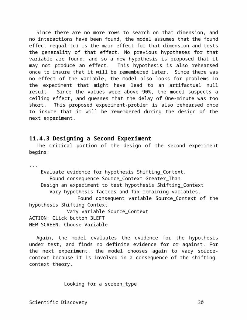
Another feature that is likely to be general is the use of contextual indexing. Many complex tasks require keeping track of both what has occurred thus far in the current situation and what has happened in previous situations. In order to access both types of information reliably and separately, chunks need to have some form of a context slot. One might further speculate that episodic and semantic memory distinctions might be related to chunks that have or do not have such context slots.
A third general feature is the use of multiple strategies and transitioning between strategies over time. As Reder (1982; 1987) and Siegler (1996) have demonstrated, performance in most domains involve multiple strategies within even the same individual. Just as our model can transition from testing a hypothesis to testing the effects of a particular variable, so did the subjects in the SPL task. Chapter 8 on choice illustrated the details of ACT-R’s views on strategy selection, and this chapter merely instantiates the use of multiple strategies within a complex domain.
A fourth feature is that the model was able to improve its performance by storing constraints on future behavior. Specifically, certain outcomes of experiments cued search for experiment problems, and experiment problems that were found produced specific recommendations for subsequent experiments. This use of stored constraints is likely to be another general feature. A yet unresolved issue is whether such constraints are best stored declaratively and used by productions which try to retrieve them later during design (as in our SPL model), or whether these constraints are better viewed as new productions created by production compilation which essentially act as “demons” to monitor the design of later experiments.
As a final point, we would like to address what this model says about the nature of the scientific enterprise itself. When all is said and done, our model is just composed of production rules and chunks like all the other models in this book. There are certainly more knowledge units and the model is incomplete in many ways that would require adding many more knowledge units. However, there is none of the “magic” that many associate with the scientific process. There is just a lot of knowledge required. The model can take different paths in solving a problem depending on momentary differences in activation levels and conflict resolution. Maybe this is what is meant by insight and intuition in science. That is, perhaps scientists are sometimes lucky and have random fluctuations in the subsymbolic quantities that cause them to explore a particularly profitable line of experimentation. However, this does not convey much credit on the scientist. What credits the scientist is to have more of the right knowledge (chunks and productions) just as this is what separated our undergraduates from domain experts. In the end, we think this ACT-R model instantiates Simon’s characterization of science:
Moreover, the insight that is supposed to be required for such work as discovery turns out to be synonymous with the familiar process of recognition; and other terms commonly used in the discussion of creative worksuch terms as “judgment,” “creativity,” or even “genius”appear to be wholly dispensable or to be definable, as insight is, in terms of mundane and well-understood concepts. (p. 376)
Scientific Discovery 30

Figure CaptionsFigure 11.1. The interface used for displaying the variables that could be manipulated and their current settings in the experiment being designed.
Figure 11.2. The interface used for selecting how many levels of a independent variable and the values for each level. In a), only one level is selected (i.e., this variable is held constant), and the constant value is “Same”. In b), two levels are selected (i.e., this variables is manipulated), and the values are “Same” and “DifferentRooms”.
Figure 11.3. The interface used for displaying the outcomes of experiments. Actual outcomes are the main entry in each cell. Predicted outcomes are in italics. The r value is the Pearson correlation between the predictions and actual outcomes.
Figure 11.4. Proportion of subjects in each group who mention the theories during experiment design (during the first experiment or during any experiment).
Figure 11.5. Percentage of undergraduate subjects varying each of variables in the first experiment as a function of whether they were explicitly testing the given theories or simply exploring the factors.
Figure 11.6. Percentage of subjects varying more than one, two, or three values.
Figure 11.7. Percentage of subjects with floor or ceiling effect experiments.
Figure 11.8. The mean number of factors varied per experiment.
Figure 11.9. Percentage of subjects making correct conclusions about each interaction given opportunity to observe the interaction (hits) and percentage of subjects making extraneous interaction conclusions (false alarms).
Figure 11.10. The model’s top-level goal structures.
Figure 11.11. Top: Percentage of undergraduate subjects varying each of variables in the first experiment as a function of whether they were explicitly testing the given theories or simply exploring the factors. Bottom: Percentage of model runs in which the model varies each of the variables in its first experiment as a function of whether the model is run with or without the production that sets the TEST-HYPOTHESIS subgoal.
Figure 11.12. Left: Percentage of subjects varying more than one, two, or three values. Right: Percentage of model runs in which the model varies more than one, two, or three values as a function of whether the model is run with or without is run with or without the production to retrieve from memory and use values from the previous experiment.
Figure 11.13. Left: The mean number of factors varied per experiment by the subjects. Right: The mean number of factors varied by the model as a function of whether the model was run with or without prior INTERACTION chunks, or both without prior INTERACTION chunks and without the production that sets the TEST-HYPOTHESIS subgoal
Scientific Discovery 31

Scientific Discovery 32
Figure 11.1
Source TaskRepetitions 3
Spacings 5 Minutes, or20 Minutes
Contexts No current selection
Tasks
Delays
Contexts
Reset
Test TaskNo current selection
No current selection
No current selection
Scientific Discovery 33

Figure 11.2
a)
Same
SourceTaskFeatures
Contexts1
b)
Same
SourceTaskFeatures
Contexts2
or Same
Scientific Discovery 34

Figure 11.3
Actual Outcome
3375
3580
r=0.88
Next Experiment
SourceContexts
TestDelays
5 Minutes 20 Minutes 2 Hours
SourceRepetitions=3
5 Minutes
20 Minutes
5 Minutes
20 Minutes
5 Minutes 20 Minutes 2 Hours
SourceSpacings
TestDelays
SourceSpacings
49
Scientific Discovery 35

Figure 11.4
Domain-ExpertsTask-Experts High-Ugrads Mid-Ugrads0
10
2030
40
5060
70
80
90100
Group
1st Experiment
Any Experiment
Scientific Discovery 36
Figure 11.5
T
T
T
T
T
T
E
EE
E
EE
Repetitions Spacing Source cntxt Test task Delay Test cntxt0
20
40
60
80
100
Factors in 1st Experiment
T Test theory
E Explore factors
Scientific Discovery 37

Figure 11.6
Scientific Discovery 38

Figure 11.7
Domain-ExpertsTask-Experts High-Ugrads Mid-Ugrads0
0.1
0.2
0.3
0.4
0.5
Group
Scientific Discovery 39
Figure 11.8
Scientific Discovery 40
Figure 11.9
Scientific Discovery 41
Figure 11.10
Scientific Discovery 42

Scientific Discovery 43

Scientific Discovery 44

Figure 11.11
T
T
T
T
T
T
E
EE
E
EE
Repetitions Spacing Source cntxt Test task Delay Test cntxt0
20
40
60
80
100T Test theory
E Explore factors
W
W W
W W W
O
O O O O O
Repetitions Spacing Source cntxt Test task Delay Test cntxt0
20
40
60
80
100W With
O Without
Data
Model
Scientific Discovery 45

Figure 11.12
1
1 1
1
1
1
2 2
2
2
2
2
3 33
3
3 3Domain-Experts
Task-Experts
High-Ugrads
Mid-Ugrads
With Without0
10
20
30
40
50
60
70
80
90
1001 Any change >1?
2 Any change >2?
3 Any change >3?
Data Model
Scientific Discovery 46
Figure 11.13
Domain-Experts
Task-Experts
High-Ugrads
Mid-Ugrads
With Interaction
Without Interaction
Without Test Hyp
1
2
3
1st Experiment
All Experiments
Data Model
Scientific Discovery 47
Table 11.1
Example program illustrating the different between holding general settings
constant (Experiment 2) and varying general settings (Experiment 2’).
Variable Experiment 1 Experiment 2 Experiment 2’
Repetitions 2 vs. 3 2 vs. 5 2 vs. 5
Spacing 10 minutes 10 minutes 2 days
Source context Same room Same room Different room
Test task Recall Recall Recognition
Delay 1 day 1 day 20 minutes
Test context Same room Same room Different mood
Scientific Discovery 48

Table 11.2
The experiments designed in the example model trace, their outcomes, and the
conclusions regarding them reached by the model.
# Design Outcome Conclusions
1Repetitions=2Spacing=1 minSource-context= Same vs. Diff-roomTest-task=StemDelay=1 minTest-context=Same
Source-contextSame 100Diff-Room 99
Maybe no effect of source-context
1min delay too short
2Repetitions=2Spacing=1 minSource-context= Same vs. Diff-roomTest-task=StemDelay=10 minTest-context=Same
Source-contextSame 64Diff-Room 64
Definitely no effect of source-context
3Repetitions=2Spacing= 1 min vs. 5 minSource-context=SameTest-task= Stem vs. RecallDelay= 10 min vs. 1 minTest-context=Same
Delay10 min Test-task Spacing Stem Recall 1 min 65 11 5 min 63 311 min Test-task Spacing Stem Recall 1 min 100 93 5 min 99 92
Maybe no effect of spacing
1 min vs 5 min too close Maybe effect of delay Maybe effect of test-task
4Repetitions=2Spacing= 1 min vs. 10 minSource-context=SameTest-task= Stem vs. RecallDelay= 10 min vs. 1 minTest-context=Same
Delay10 min Test-task Spacing Stem Recall 1 min 64 12 10 min 63 391 min Test-task Spacing Stem Recall 1 min 99 92 10 min 100 92
Definitely no main effect of spacing
Definitely effect of delay Definitely effect of test-
task
Scientific Discovery 49
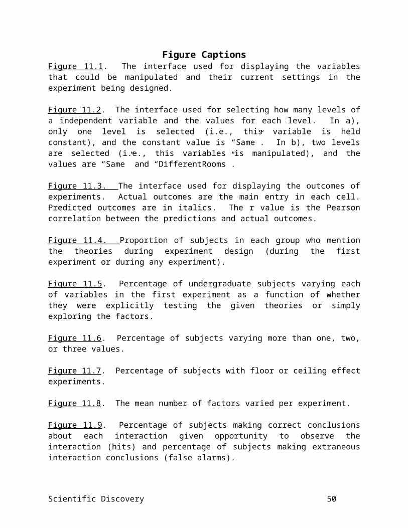
Scientific Discovery 50

Table 11.3
During the design of each experiment, the proportion of transitions from one
variable (Rows) to another variable (Columns) including returns to the same
variable and finishing of the experiment design (Stop), separately for experts and
undergraduates.
Experts Repetition Spacing SourceContext
TestTask
Delay TestContext
Stop
Repetition 4 52 11 16 11 1 5
Spacing 38 5 41 9 7 0 0
Source Context 4 17 7 32 5 29 6
Test Task 3 0 12 3 60 9 14
Delay 3 2 3 19 11 51 11
Test Context 13 0 16 6 18 5 43
Undergrads Repetition Spacing SourceContext
TestTask
Delay TestContext
Stop
Repetition 3 77 6 7 2 1 4
Spacing 12 5 65 6 8 0 3
Source Context 1 6 4 62 4 19 4
Test Task 4 3 6 5 72 3 8
Delay 4 4 4 9 7 62 10
Test Context 5 5 8 11 13 8 49
Scientific Discovery 51


![Working Draft Dan Bothell - ACT-Ract-r.psy.cmu.edu/wordpress/wp-content/themes/ACT-R/actr7/... · then you should probably start with the ACT-R tutorial.] ... LispWorks, Clozure Common](https://static.fdocuments.us/doc/165x107/5b8922767f8b9ae7298baf5a/working-draft-dan-bothell-act-ract-rpsycmueduwordpresswp-contentthemesact-ractr7.jpg)