Ch. 15 Forecasting

Ch. 15 Forecasting(March 25, 2019)

Having considered in Chapter 14 some of the properties of ARMA models, we now

show how they may be used to forecast future values of an observed time series. For

the present we proceed as if the model were known exactly.1

One of the important problems in time series analysis is the following: Given T

observations on a realization, predict the (T + s)th observation in the realization,

where s is a positive integer. The prediction is sometime called the forecast of the

(T + s)th observation.

Forecasting is an important concept for the studies of time series analysis. In the

scope of regression model we usually has an existing economic theory model for us to

estimate their parameters. The estimated coefficients have already a role to play such

as to confirm some economic theories. Therefore, to forecast or not from this estimated

model depends on researcher’s own interest. However, the estimated coefficients from

a time series model have no significant meaning to economic theory. An important role

that a time series analysis is therefore to be able to forecast precisely from this pure

mechanical model.

1 Principle of Forecasting

1.1 Forecasts Based on Conditional Expectations (With a Known Model)

Suppose we are interested in forecasting the value of a variables Yt+1 based on a set of

variables xt observed at date t. For example, we might want to forecast Yt+1 based on

1That is, the model we assume is a correct specification and its parameters are known.

1

Ch.15 Forecasting 1 PRINCIPLE OF FORECASTING

its m most recent values. In this case, xt = [Yt, Yt−1, ...., Yt−m+1]′.

Let Yt+1|t denote a forecast of Yt+1 based on xt (a function of xt, depending on

how they are realized). To evaluate the usefulness of this forecast, we need to specify

a loss function. A quadratic loss function means choosing the forecast Y ∗t+1|t so as to

minimize

MSE(Yt+1|t) = E(Yt+1 − Yt+1|t)2,

which is known as the mean squared error.

Theorem.The smallest mean squared error of in the forecast Yt+1|t is the (statistical) expectation

of Yt+1 conditional on xt:

Y ∗t+1|t = E(Yt+1|xt).

Proof:Let g(xt) be a forecasting function of Yt+1 other then the conditional expectation

E(Yt+1|xt). Then the MSE associated with g(xt) would be

E[Yt+1 − g(xt)]2 = E[Yt+1 − E(Yt+1|xt) + E(Yt+1|xt)− g(xt)]

2

= E[Yt+1 − E(Yt+1|xt)]2

+2E{[Yt+1 − E(Yt+1|xt)][E(Yt+1|xt)− g(xt)]}

+E{E[(Yt+1|xt)− g(xt)]2}.

Denote ηt+1 ≡ {[Yt+1 − E(Yt+1|xt)][E(Yt+1|xt)− g(xt)]} we have

E(ηt+1|xt) = [E(Yt+1|xt)− g(xt)]× E([Yt+1 − E(Yt+1|xt)]|xt)

= [E(Yt+1|xt)− g(xt)]× 0

= 0.

By laws of iterated expectation, it follows that

E(ηt+1) = ExtE(E[ηt+1|xt]) = 0.

Therefore we have

E[Yt+1 − g(xt)]2 = E[Yt+1 − E(Yt+1|xt)]2 + E{E[(Yt+1|xt)− g(xt)]

2}. (15-1)

r 2018 by Prof. Chingnun Lee 2 Ins.of Economics,NSYSU,Taiwan


The second term on the right hand side of (15-1) cannot be made smaller than zero

and the first term does not depend on g(xt). The function g(xt) that can makes the

mean square error (15-1) as small as possible is the function that sets the second term

in (15-1) to zero:

g(xt) = E(Yt+1|xt).

The MSE of this optimal forecast is thus

E[Yt+1 − g(xt)]2 = E[Yt+1 − E(Yt+1|xt)]2.

�

1.2 Forecasts Based on Linear Projection (Without a Known Model)

Suppose we now consider only the class of forecast Yt+1 that is a linear function of xt:

Yt+1|t = α′xt.

Definition :

The forecast α′xt is called the linear projection of Yt+1 on xt if the forecast error

(Yt+1 −α′xt) is uncorrelated with xt, i.e.

E[(Yt+1 −α′xt)x′t] = 0′. (15-2)

�

Theorem.The linear projection produces the smallest mean squared error among the class of

linear forecasting rule.

Proof:Let g′xt be any arbitrary linear forecasting function of Yt+1. Then the MSE associated



with g′xt would be

E[Yt+1 − g′xt]2 = E[Yt+1 −α′xt + α′xt − g′xt]

2

= E[Yt+1 −α′xt]2

+2E{[Yt+1 −α′xt][α′xt − g′xt]}

+E[α′xt − g′xt]2.

Denote ηt+1 ≡ {[Yt+1 −α′xt][α′xt − g′xt]} we have

E(ηt+1) = E{[Yt+1 −α′xt][(α− g)′xt]}

= (E[Yt+1 −α′xt]x′t)[α− g]

= 0′[α− g]

= 0.

Therefore we have

E[Yt+1 − g′xt]2 = E[Yt+1 −α′xt)]

2 + E[α′xt − g′xt]2. (15-3)

The second term on the right hand side of (15-3) cannot be made smaller than zero

and the first term does not depend on g′xt. The function g′xt that can makes the

mean square error (15-3) as small as possible is the function that sets the second term

in (15-3) to zero:

g′xt = α′xt.

The MSE of this optimal forecast is

E[Yt+1 − g′xt]2 = E[Yt+1 −α′xt]

2.

�

Notation.For α′xt is a linear projection of Yt+1 on xt, we will use the notation

P (Yt+1|xt) = α′xt,

to indicate the linear projection of Yt+1 on xt. �

Notice that

MSE[P (Yt+1|xt)] ≥MSE[E(Yt+1|xt)],



since the conditional expectation offers the best possible forecast.

For most applications a constant term will be included in the projection. We will

use the symbol E to indicate a linear projection on a vector of random variables xt

along a constant term:

E(Yt+1|xt) ≡ P (Yt+1|1,xt).


Ch.15 Forecasting2 FORECAST ARMA MODEL WITH INFINITE OBSERVATIONS

2 Forecast ARMA Model with Infinite Observations

Recall that a general stationary and invertible ARMA(p, q) process is written in this

form:

φ(L)(Yt − µ) = θ(L)εt, (15-4)

where φ(L) = 1− φ1L− φ2L2 − ...− φpLp, θ(L) = 1 + θ1L+ θ2L

2 + ...+ θqLq and all

the roots of φ(L) = 0 and θ(L) = 0 lie outside the unit circle.

2.1 Forecasting Based on Lagged ε′s, MA(∞) form

Assume that the lagged εt is observed directly, then the following principle is useful

in the manipulating the forecasting in the subsequence. Consider an MA(∞) form of

(15-4):

Yt − µ = ϕ(L)εt (15-5)

with εt white noise and

ϕ(L) = θ(L)φ−1(L) =∞∑j=0

ϕjLj,

where ϕ0 = 1 and∑∞

j=0 |ϕj| <∞.

Suppose that we have an infinite number of observations on ε through date t, that

is {εt, εt−1, εt−2, ....}, and further know the value of µ and {ϕ1, ϕ2, ...}. Say we want to

forecast the value of Yt+s from now. Note that (15-5) implies

Yt+s = µ+ εt+s + ϕ1εt+s−1 + ...+ ϕs−1εt+1 + ϕsεt

+ϕs+1εt−1 + ....

We consider the best linear forecast since the ARMA model we considered so far is

covariance-stationary, no assumption is made on their distribution so we cannot form

conditional expectation. The best linear forecast takes the form2

E(Yt+s|εt, εt−1, ...) = µ+ ϕsεt + ϕs+1εt−1 + ....

= [µ, ϕs, ϕs+1, ...][1, εt, εt−1, ...]′

= α′xt. (15-6)

2You cannot use conditional expectation that E(εt+i|εt, εt−1, ..) = 0 for i = 1, 2, · · · , s since weonly assume that εt is uncorrelated which do not imply that they are independent.



That is, the unknown future ε’s are set to their expected value of zero. The error

associated with this forecast is uncorrelated with xt = [1, εt, εt−1, ...]′, or

E{xt · [Yt+s − E(Yt+s|εt, εt−1, ...)]}

= E

1εtεt−1...

(εt+s + ϕ1εt+s−1 + ...+ ϕs−1εt+1)

= 0.

The mean squared error associated with this forecast is

E[Yt+s − E(Yt+s|εt, εt−1, ...)]2 = (1 + ϕ21 + ϕ2

2 + ...+ ϕ2s−1)σ

2.

Example .

For an MA(q) process, the optimal linear forecast is

E(Yt+s|εt, εt−1, ...] =

{µ+ θsεt + θs+1εt−1 + ...+ θqεt−q+s for s = 1, 2, ..., q

µ for s = q + 1, q + 2, ...

The MSE isσ2, for s = 1

(1 + θ21 + θ22 + ...+ θ2s−1)σ2, for s = 2, 3, ..., q

((1 + θ21 + θ22 + ...+ θ2q)σ2, for s = q + 1, q + 2, ....

The MSE increase with the forecast horizon s up until s = q. If we try to forecast

an MA(q) farther than q periods into the future, the forecast is simply the uncondi-

tional mean of the series (E(Yt+s) = µ)) and the MSE is the unconditional variance of

the series (V ar(Yt+s) = (1 + θ21 + θ22 + ...+ θ2q)σ2). �

A compact lag operator expression for the forecast in (15-6) is sometimes used.

Rewrite Yt+s as in (15-5) as

Yt+s = µ+ ϕ(L)εt+s

= µ+ ϕ(L)L−sεt.

Consider polynomial that ϕ(L) are divided by Ls:

ϕ(L)

Ls= L−s + ϕ1L

1−s + ϕ2L2−s + ...+ ϕs−1L

−1 + ϕsL0

+ϕs+1L1 + ϕs+2L

2 + ....



The annihilation operator is to replace negative powers of L in ϕ(L)Ls by zero. For

example,[ϕ(L)

Ls

]+

= ϕsL0 + ϕs+1L

1 + ϕs+2L2 + ....

Therefore the optimal forecast (15-6) could be written in lag operator notation as

E(Yt+s|εt, εt−1, ...] = µ+ ϕsεt + ϕs+1εt−1 + ....

= µ+ (ϕsL0 + ϕs+1L

1 + ϕs+2L2 + ....)εt

= µ+

[ϕ(L)

Ls

]+

εt. (15-7)

2.2 Forecasting Based on Lagged Y ′s

The previous forecasts were based on the assumption that εt is observed directly. In

the usual forecasting situation, we actually have observation on lagged Y ′s, not lagged

ε′s. Suppose that the general ARMA(p, q) has an AR(∞) representation given by

η(L)(Yt − µ) = εt (15-8)

with εt white noise and

η(L) = θ−1(L)φ(L) =∞∑j=0

ηjLj = ϕ−1(L),

where η0 = 1 and∑∞

j=0 |ηj| <∞.

Under these conditions, we can substitute (15-8) into (15-7) to obtain the forecast

of Yt+s as a function of lagged Y ′s:

E(Yt+s|Yt, Yt−1, ...] = µ+

[ϕ(L)

Ls

]+

η(L)(Yt − µ) (15-9)

or

E(Yt+s|Yt, Yt−1, ...] = µ+

[ϕ(L)

Ls

]+

1

ϕ(L)(Yt − µ). (15-10)

Equation (15-10) is known as the Wiener-Kolmogorov prediction formula.



2.2.1 Forecasting an AR(1) Process

Therefore are two ways to forecast a AR(1) process. They are:

(a). By Wiener-Kolmogorov prediction formula:

For the covariance stationary AR(1) process, we have

ϕ(L) =1

1− φL= 1 + φL+ φ2L2 + φ3L3 + ...

and [ϕ(L)

Ls

]+

= φs + φs+1L1 + φs+2L2 + ... =φs

1− φL.

The optimal linear s-period ahead forecast for a stationary AR(1) process is

therefore:

E(Yt+s|Yt, Yt−1, ...] = µ+φs

1− φL(1− φL)(Yt − µ)

= µ+ φs(Yt − µ).

The forecast decays geometrically from (Yt−µ) toward µ as the forecast horizon

s increase.

(b). By Recursive Substitution and Lag operator:

The AR(1) process can be represented as (using (13-3) on Ch. 13)

Yt+s − µ = φs(Yt − µ) + φs−1εt+1 + φs−2εt+2 + ...+ φεt+s−1 + εt+s,

Setting E(εt+h) = 0, h = 1, 2, ..., s, the optimal linear s-period ahead forecast for

a stationary AR(1) process is therefore:

E(Yt+s|Yt, Yt−1, ...] = µ+ φs(Yt − µ),

with forecast error φs−1εt+1 +φs−2εt+2 + ...+φεt+s−1 +εt+s, which is uncorrelated

with the forecast Yt(= µ+ εt + φ1εt−1 + φ2εt−2 + ....). �



The MSE of this forecast is

E(φs−1εt+1 + φs−2εt+2 + ...+ φεt+s−1 + εt+s)2 = (1 + φ2 + φ4 + ...+ φ2(s−1))σ2.

Notice that this grows with s and asymptotically approach σ2/(1−φ2), the uncon-

ditional variance of Y .3

2.2.2 Forecasting an AR(p) Process

(a). By Recursive substitution and Lag operator:

Following (13-11) in Chapter 13, the value of Y at t+ s of an AR(p) process can

be represented as

Yt+s − µ = f s11(Yt − µ) + f s12(Yt−1 − µ) + ...+ f s1p(Yt−p+1 − µ)

+f s−111 εt+1 + f s−211 εt+2 + ...+ f 111εt+s−1 + εt+s,

where f j11 is the (1, 1) elements of Fj, in which

F ≡

φ1 φ2 φ3 . . φp−1 φp1 0 0 . . 0 00 1 0 . . 0 0. . . . . . .. . . . . . .. . . . . . .0 0 0 . . 1 0

.

Setting E(εt+h) = 0, h = 1, 2, ..., s, the optimal linear s-period ahead forecast for

a stationary AR(p) process is therefore:

E(Yt+s|Yt, Yt−1, ...] = µ+ f s11(Yt − µ) + f s12(Yt−1 − µ) + ...+ f s1p(Yt−p+1 − µ).

(15-11)

The associated forecast error is

Yt+s − E(Yt+s) = f s−111 εt+1 + f s−211 εt+2 + ...+ f 111εt+s−1 + εt+s.

3That is, with the information of Yt to forecast Yt+s, the MSE could never be larger than theunconditional variance of Yt+s.



(b). By Law of Iterated Projection:

The easiest way to calculate the forecast in (15-11) is through a simple recursion

called law of iterated projection. Suppose at date t we wanted to make a one-

period-ahead forecast of Yt+1. The optimal (by setting s = 1 in (15-11)) is clearly

E(Yt+1 − µ|Yt, Yt−1, ...] = φ1(Yt − µ) + φ2(Yt−1 − µ) + ...+ φp(Yt−p+1 − µ).

(15-12)

Next consider a two-period-ahead forecast. Suppose that at date t + 1 we were

to make a one-period-ahead forecast of Yt+2. Replacing t with t + 1 in (15-12)

give s the optimal forecast as

E(Yt+2 − µ|Yt+1, Yt, ...] = φ1(Yt+1 − µ) + φ2(Yt − µ) + ...+ φp(Yt−p+2 − µ).

(15-13)

The law of iterated projections asserts that if this date t + 1 forecast of Yt+2 is

projected on date t information, the results is the data t forecast of Yt+2. At date

t the values Yt, Yt−1, ...., Yt−p+2 in (15-13) are known . Thus

E(Yt+2 − µ|Yt, Yt−1, ...] = φ1E(Yt+1 − µ|Yt, Yt−1, ...] + φ2(Yt − µ) + ...+

φp(Yt−p+2 − µ). (15-14)

The s-period-ahead forecast of an AR(p) process can therefore be obtained by

iterating on

E(Yt+j − µ|Yt, Yt−1, ...] = φ1E(Yt+j−1 − µ|Yt, Yt−1, ...] + φ2E(Yt+j−2 −

µ|Yt, Yt−1, ...] + ...+ φpE(Yt+j−p − µ|Yt, Yt−1, ...]

(15-15)

for j = 1, 2, ..., s where

E(Yτ − µ|Yt, Yt−1, ...] = Yτ , for τ ≤ t. �

It is important to note that to forecast an AR(p) process, an optimal s-period-ahead

linear forecast based on an infinite number of observations {Yt, Yt−1, ...} in fact make

use of only the p most recent value {Yt, Yt−1, .., Yt−p+1}.



2.2.3 Forecasting an MA(1) Process

An invertible MA(1) process:

Yt − µ = (1 + θL)εt, with |θ| < 1.

(a). By the Wiener-Kolmogorov formula:

Using the Wiener-Kolmogorov formula we have

Yt+s|t = µ+

[1 + θL

Ls

]+

1

1 + θL(Yt − µ).

To forecast an MA(1) process one-period-ahead (s = 1),[1 + θL

L1

]+

= θ,

and so

Yt+1|t = µ+θ

1 + θL(Yt − µ)

= µ+ θ(Yt − µ)− θ2(Yt−1 − µ) + θ3(Yt−2 − µ)− ....

To forecast an MA(1) process for s = 2, 3, ... periods into the future,[1 + θL

Ls

]+

= 0 for s = 2, 3, ...,

an so

Yt+s|t = µ for s = 2, 3, ....

(b). By Recursive Substitution:

An MA(1) process at period t+ 1 is

Yt+1 − µ = εt+1 + θεt.

At period t, E(εt+s) = 0, s = 1, 2, .... The optimal linear 1-period-ahead forecast

for a stationary MA(1) process is therefore:

Yt+1|t = µ+ θεt

= µ+ θ(1 + θL)−1(Yt − µ)

= µ+ θ(Yt − µ)− θ2(Yt−1 − µ) + θ3(Yt−2 − µ)− ....



An MA(1) process at period t+ s is

Yt+s − µ = εt+s + θεt+s−1,

To forecast an MA(1) process for s = 2, 3, ... periods into the future therefore is

Yt+s|t = µ for s = 2, 3, .... �

2.2.4 Forecasting an MA(q) Process

For an invertible MA(q) process,

(Yt − µ) = (1 + θ1L+ θ2L2 + ...+ θqL

q)εt,

the forecast becomes

Yt+s|t = µ+

[1 + θ1L+ θ2L

2 + ...+ θqLq

Ls

]+

1

1 + θ1L+ θ2L2 + ...+ θqLq(Yt − µ).

Now [1 + θ1L+ θ2L

2 + ...+ θqLq

Ls

]+

=

{θs + θs+1L+ θs+2L

2 + ...+ θqLq−s, for s = 1, 2, ..., q

0, for s = q + 1, q + 2, ...

Thus for horizons of s = 1, 2, ..., q, the forecast is given by

Yt+s|t = µ+ (θs + θs+1L+ θs+2L2 + ...+ θqL

q−s)1

1 + θ1L+ θ2L2 + ...+ θqLq(Yt − µ).

A forecast farther then q periods into the future is simply the unconditional mean µ.

It is important to note that to forecast an MA(q) process, an optimal s (s ≤ q)-

period-ahead linear forecast would in principle requires all of the historical value of Y

{Yt, Yt−1, ...}.



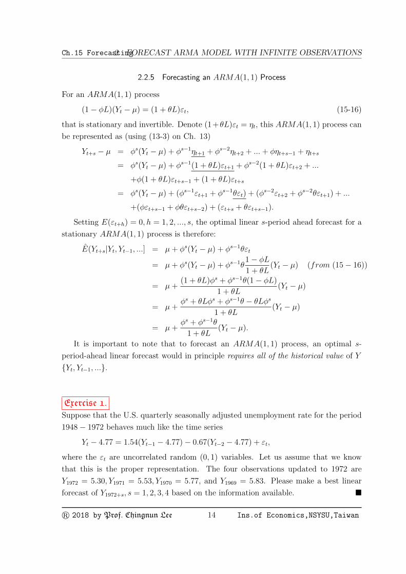
2.2.5 Forecasting an ARMA(1, 1) Process

For an ARMA(1, 1) process

(1− φL)(Yt − µ) = (1 + θL)εt, (15-16)

that is stationary and invertible. Denote (1+θL)εt = ηt, this ARMA(1, 1) process can

be represented as (using (13-3) on Ch. 13)

Yt+s − µ = φs(Yt − µ) + φs−1ηt+1 + φs−2ηt+2 + ...+ φηt+s−1 + ηt+s

= φs(Yt − µ) + φs−1(1 + θL)εt+1 + φs−2(1 + θL)εt+2 + ...

+φ(1 + θL)εt+s−1 + (1 + θL)εt+s

= φs(Yt − µ) + (φs−1εt+1 + φs−1θεt) + (φs−2εt+2 + φs−2θεt+1) + ...

+(φεt+s−1 + φθεt+s−2) + (εt+s + θεt+s−1).

Setting E(εt+h) = 0, h = 1, 2, ..., s, the optimal linear s-period ahead forecast for a

stationary ARMA(1, 1) process is therefore:

E(Yt+s|Yt, Yt−1, ...] = µ+ φs(Yt − µ) + φs−1θεt

= µ+ φs(Yt − µ) + φs−1θ1− φL1 + θL

(Yt − µ) (from (15− 16))

= µ+(1 + θL)φs + φs−1θ(1− φL)

1 + θL(Yt − µ)

= µ+φs + θLφs + φs−1θ − θLφs

1 + θL(Yt − µ)

= µ+φs + φs−1θ

1 + θL(Yt − µ).

It is important to note that to forecast an ARMA(1, 1) process, an optimal s-

period-ahead linear forecast would in principle requires all of the historical value of Y

{Yt, Yt−1, ...}.

Exercise 1.Suppose that the U.S. quarterly seasonally adjusted unemployment rate for the period

1948− 1972 behaves much like the time series

Yt − 4.77 = 1.54(Yt−1 − 4.77)− 0.67(Yt−2 − 4.77) + εt,

where the εt are uncorrelated random (0, 1) variables. Let us assume that we know

that this is the proper representation. The four observations updated to 1972 are

Y1972 = 5.30, Y1971 = 5.53, Y1970 = 5.77, and Y1969 = 5.83. Please make a best linear

forecast of Y1972+s, s = 1, 2, 3, 4 based on the information available. �


Ch.15 Forecasting 3 FORECAST BASED ON FINITE M OBSERVATIONS

3 Forecast Based on Finite m Observations

The section continues to assume that population parameters are known with certainty,

but develops forecasts based on a finite m observations, {Yt, Yt−1, ..., Yt−m+1}

3.1 Approximations to Optimal Forecast In ARMA Process

For forecasting an AR(p) process, an optimal s-period-ahead linear forecast based on

an infinite number of observations {Yt, Yt−1, · · · } in fact make use of only the p most

recent value {Yt, Yt−1, · · · , Yt−p+1}. For an MA or ARMA process, however, we would

require in principle all of the historical value of Y in order to implement the formula

of the proceeding section.

In reality we do not have infinite number of observations for forecasting. One

approach to forecasting based on a finite number of observations is to act as if pre-

sample Y ’s were all equal to its mean value µ (or ε = 0). This idea is thus to use the

approximation

E(Yt+s|1, Yt, Yt−1, ...) ∼= E(Yt+s|Yt, Yt−1, ..., Yt−m+1;Yt−m = µ, Yt−m−1 = µ, ...).

For example in the forecasting of an MA(1) process, the 1 period ahead forecast

Yt+1|t = µ+ θ(Yt − µ)− θ2(Yt−1 − µ) + θ3(Yt−2 − µ)− ....

is approximated by

Yt+1|t = µ+ θ(Yt − µ)− θ2(Yt−1 − µ) + θ3(Yt−2 − µ)− ....+ (−1)m−1θm(Yt−m+1 − µ).

(15-17)

For m large and |θ| small (then the real difference between Y and µ will multiply a

small and smaller number), this clearly gives an excellent approximation. For |θ| closer

to unity, the approximation may be poor.

Example .

To forecast a MA(1) process, most software package is doing this way: because Yt =

εt + θεt−1, therefore

Yt+1|t = θεt,



where the realization of εt, εt, is recurved from

εt = Yt − θεt−1, t = 1, 2, ...,

with the assumption that ε0 = 0. For example,

Y4|3 = θε3

= θ(Y3 − θε2)

= θY3 − θ2(Y2 − θε1)

= θY3 − θ2Y2 + θ3ε1

= θY3 − θ2Y2 + θ3Y1. (15-18)

Substitute m = t = 3 and µ = 0 into (15-17), we obtain (15-18). �

3.2 Exact Finite-Sample Forecast by Linear Projection

An alternative approach is to calculate the exact projection of Yt+1 on its m most

recent values.4 Let

xt =

1YtYt−1...

Yt−m+1

We thus seek a linear forecast of the form

E(Yt+1|xt) = α′(m)xt = α

(m)0 + α

(m)1 Yt + α

(m)2 Yt−1 + ...+ α(m)

m Yt−m+1. (15-19)

The coefficient relating Yt+1 to Yt in a projection of Yt+1 on the m most recent value

of Y is denoted α(m)1 in (15-19). This will in general be different from the coefficient

relating Yt+1 to Yt in a projection of Yt+1 on the (m + 1) most recent value of Y ; the

latter coefficient would be denoted α(m+1)1 .

From (15-2) we know that

E(Yt+1x′t) = α′E(xtx

′t),

4So we do not need to assume any model such as ARMA here.



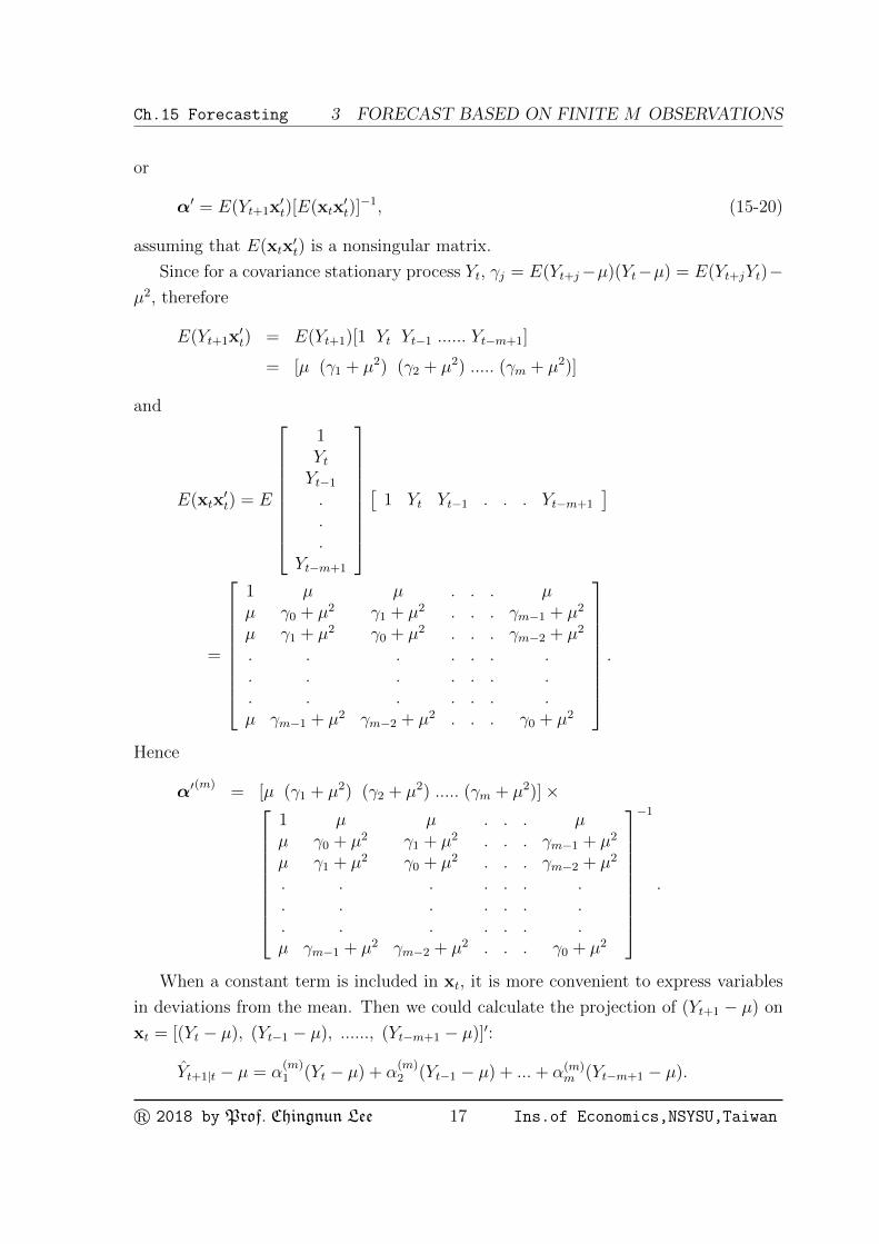
or

α′ = E(Yt+1x′t)[E(xtx

′t)]−1, (15-20)

assuming that E(xtx′t) is a nonsingular matrix.

Since for a covariance stationary process Yt, γj = E(Yt+j−µ)(Yt−µ) = E(Yt+jYt)−µ2, therefore

E(Yt+1x′t) = E(Yt+1)[1 Yt Yt−1 ...... Yt−m+1]

= [µ (γ1 + µ2) (γ2 + µ2) ..... (γm + µ2)]

and

E(xtx′t) = E

1YtYt−1...

Yt−m+1

[

1 Yt Yt−1 . . . Yt−m+1

]

=

1 µ µ . . . µµ γ0 + µ2 γ1 + µ2 . . . γm−1 + µ2

µ γ1 + µ2 γ0 + µ2 . . . γm−2 + µ2

. . . . . . .

. . . . . . .

. . . . . . .µ γm−1 + µ2 γm−2 + µ2 . . . γ0 + µ2

.

Hence

α′(m)

= [µ (γ1 + µ2) (γ2 + µ2) ..... (γm + µ2)]×

1 µ µ . . . µµ γ0 + µ2 γ1 + µ2 . . . γm−1 + µ2

µ γ1 + µ2 γ0 + µ2 . . . γm−2 + µ2

. . . . . . .

. . . . . . .

. . . . . . .µ γm−1 + µ2 γm−2 + µ2 . . . γ0 + µ2

−1

.

When a constant term is included in xt, it is more convenient to express variables

in deviations from the mean. Then we could calculate the projection of (Yt+1 − µ) on

xt = [(Yt − µ), (Yt−1 − µ), ......, (Yt−m+1 − µ)]′:

Yt+1|t − µ = α(m)1 (Yt − µ) + α

(m)2 (Yt−1 − µ) + ...+ α(m)

m (Yt−m+1 − µ).



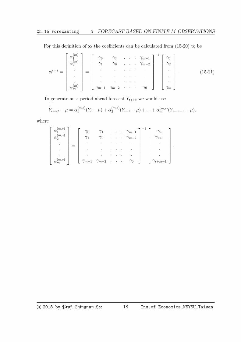
For this definition of xt the coefficients can be calculated from (15-20) to be

α(m) =

α(m)1

α(m)2

.

.

.

α(m)m

=

γ0 γ1 . . . γm−1γ1 γ0 . . . γm−2. . . . . .. . . . . .. . . . . .

γm−1 γm−2 . . . γ0

−1 γ1γ2...γm

. (15-21)

To generate an s-period-ahead forecast Yt+s|t we would use

Yt+s|t − µ = α(m,s)1 (Yt − µ) + α

(m,s)2 (Yt−1 − µ) + ...+ α(m,s)

m (Yt−m+1 − µ),

where

α(m,s)1

α(m,s)2

.

.

.

α(m,s)m

=

γ0 γ1 . . . γm−1γ1 γ0 . . . γm−2. . . . . .. . . . . .. . . . . .

γm−1 γm−2 . . . γ0

−1 γsγs+1

.

.

.γs+m−1

.


Ch.15 Forecasting 4 SUMS OF ARMA PROCESS

4 Sums of ARMA Process

This section explores the nature of series that result from adding two different ARMA

process together.

4.1 Sum of an MA(1) Process and White Noise

Suppose that a series Xt follows a zero-mean MA(1) process:

Xt = ut + δut−1,

where ut is white noise with variance σ2u. The autocovariance of Xt are thus

E(XtXt−j) =

(1 + δ2)σ2

u for j = 0δσ2

u for j = ±10 otherwise.

(15-22)

Let vt indicate a separate white noise series with variance σ2v . Suppose, furthermore,

that v and u are uncorrelated at all leads and lags, i.e.,

E(utvt−j) = 0 for all j,

implying that

E(Xtvt−j) = o for all j. (15-23)

Let an observed series Yt represent the sum of the MA(1) and the white noise

process:

Yt = Xt + vt

= ut + δut−1 + vt. (15-24)

The question now posed is: What are the time series properties of Y ?

Clearly, Yt has mean zero, and its autocovariances can be deduced from (15-22)

through (15-23):

E(YtYt−j) = E(Xt + vt)(Xt−j + vt−j)

= E(XtXt−j) + E(vtvt−j)

=

(1 + δ2)σ2

u + σ2v , for j = 0;

δσ2u, for j = ±1;

0, otherwise.(15-25)



Thus, the sum, Xt + vt, is covariance-stationary, and its autocovariances are zero

beyond one lags, as those for an MA(1). We might naturally then ask whether there

exist a zero-mean MA(1) represent for Y ,

Yt = εt + θεt−1, (15-26)

with

E(εtεt−j) =

{σ2, for j = 0;0, otherwise,

(15-27)

whose autocovariance match those implied by (15-25). The autocovariance of (15-26)

would be given by

E(YtYt−j) =

(1 + θ2)σ2 for j = 0

θσ2 for j = ±10 otherwise.

In order to be consistent with (15-25), it would be the case that

(1 + θ2)σ2 = (1 + δ2)σ2u + σ2

v (15-28)

and

θσ2 = δσ2u. (15-29)

Taking the value5 associated with the invertible representation (θ∗, σ2∗) which is

solved from (15-28) and (15-29) simultaneously. Let us consider whether (15-26) could

indeed characterize the data Yt generated by (15-24). This would require

(1 + θ∗L)εt = (1 + δL)ut + vt,

or

εt = (1 + θ∗L)−1[(1 + δL)ut + vt]

= (ut − θ∗ut−1 + θ∗2ut−2 − θ∗3ut−3 + · · · )

+δ(ut−1 − θ∗ut−2 + θ∗2ut−3 − θ∗3ut−4 + · · · )

+(vt − θ∗vt−1 + θ∗2vt−2 − θ∗3vt−3 + · · · ). (15-30)

5Two value of θ that satisfy (15-28) and (15-29) can be found from the quadratic formula:

θ =[(1 + δ2) + (σ2

v/σ2u)]±

√[(1 + δ2) + (σ2

v/σ2u)]2 − 4δ2

2δ



The series εt defined in (15-30) is a distributed lag on past value of u and v, so it

might seem to possess a rich autocorrelation structure. In fact, it turns out to be white

noise ! To see this, note from (15-25) that the autocovariance-generating function of

Y can be written

gY (z) = δσ2uz−1 + [(1 + δ2)σ2

u + σ2v ]z

0 + δσ2uz

1

= σ2u(1 + δz)(1 + δz−1) + σ2

v , (15-31)

so the autocovariance-generating function of εt = (1 + θ∗L)−1Yt is

gε(z) =σ2u(1 + δz)(1 + δz−1) + σ2

v

(1 + θ∗z)(1 + θ∗z−1). (15-32)

But θ∗ and σ∗2 were chosen so as to make the autocovariance-generating function of

(1 + θ∗L)εt, namely,

(1 + θ∗z)σ∗2(1 + θ∗z−1), (15-33)

identical to the right side of (15-31). Thus, (15-32) is simply equal to

gε(z) = σ2∗,

a white noise series.

To summarize, adding an MA(1) process to a white noise series with which it is

uncorrelated at all leads and lags produce a new MA(1) process characterized by (15-

26).

4.2 Sum of Two Independent Moving Average Process

As a necessary preliminary to what follows, consider a stochastic process Wt, which is

the sum of two independent moving average processes of order q1 and q2, respectively.

That is,

Wt = θ1(L)ut + θ2(L)vt,

where θ1(L) and θ2(L) are polynomials in L, of order q1 and q2, and the white noise

processes ut and vt have zero means and are mutually uncorrelated at all lead and lags.

Suppose that q = max(q1, q2); then it is clear that the autocovariance function γj for



Wt must be zero for j > q.6 It follows that there exists a representation of Wt as a

single moving average process of order q:

Wt = θ3(L)εt, (15-34)

where εt is a white noise process with mean zero. Thus the sum of two uncorrelated

moving average processes is another moving average process, whose order is the same

as that of the component process of higher order.

4.3 Sum of an ARMA(p, q) Plus White Noise

Consider the general stationary and invertible ARMA(p, q) model

φ(L)Xt = θ(L)ut,

where ut is a white noise process with variance σ2u. Let vt indicate a separate white

noise series with variance σ2v . Suppose, furthermore, that v and u are uncorrelated at

all leads and lags.

Let an observed series Yt represent the sum of the ARMA(p, q) and the white noise

process:

Yt = Xt + vt. (15-35)

In general we have

φ(L)Yt = φ(L)Xt + φ(L)vt

= θ(L)ut + φ(L)vt.

Let q∗ = max(q, p) and from (15-34) we have that Yt is an ARMA(p, q∗) process.

6To see this, let Wt = Xt + Yt, then

γWj = E(WtWt−j) = E(Xt + Yt)(Xt−j + Yt−j)

= E(XtXt−j)(YtYt−j)

=

{γXj + γYj for j = 0,±1,±2, ..., ±q,

0 otherwise.



4.4 Adding Two Autoregressive Processes

Suppose now that Xt are AR(p1) and Wt are AR(p2) process:

φ1(L)Xt = ut

φ2(L)Wt = vt, (15-36)

where ut and vt are uncorrelated white noise at all lead and lags. Again suppose that

we observe

Yt = Xt +Wt,

we wish to determine the nature of the observed process Yt.

From (15-36) we have

φ2(L)φ1(L)Xt = φ2(L)ut

φ1(L)φ2(L)Wt = φ1(L)vt,

then

φ1(L)φ2(L)(Xt +Wt) = φ1(L)vt + φ2(L)ut

or

φ1(L)φ2(L)Yt = φ1(L)vt + φ2(L)ut.

Therefore Yt is an ARMA(p1 + p2,max{p1, p2}) process from (15-34).


Ch.15 Forecasting 5 WOLD’S DECOMPOSITION

5 Wold’s Decomposition

All of the covariance stationary ARMA process considered in Chapter 14 can be written

in the form

Yt = µ+∞∑j=0

ϕjεt−j, (15-37)

where εt is a white noise process and∑∞

j=0 ϕ2j <∞ with ϕ0 = 1.

One might think that we are able to write all these processes in the form of (15-

37) because the discussion was restricted to a convenient class of models (parametric

ARMA model). However, the following result establishes that the representation (15-

37) is in fact fundamental for any covariance-stationary time series.

Theorem (Wold’s Decomposition):

Let Yt be any covariance stationary stochastic process with EYt = 0. Then it can be

written as

Yt =∞∑j=0

ϕjεt−j + ηt, (15-38)

where ϕ0 = 1 and where∑∞

j=0 ϕ2j < ∞, Eε2t = σ2 ≥ 0, E(εtεs) = 0 for t 6= s,

Eεt = 0 and Eεtηs = 0 for all t and s; and ηt is a process that can be predicted

arbitrary well by a linear function of only past value of Yt, i.e., ηt is linearly determin-

istic.7 Furthermore, εt = Yt− E(Yt|Yt−1, Yt−2, · · · ), i.e. the term εt is a white noise and

represents the error made in forecasting Yt on the basis of a linear function of lagged Y .

Proof:See Sargent (1987, pp. 286-90) or Fuller (1996, pp. 94-98), or Brockwell and Davis

(1991, pp. 187-89). �

Wold’s decomposition is important for us because it provides an explanation of the

sense in which ARMA model (stochastic difference equation) provide a general model

for the indeterministic part of any univariate stationary stochastic process, and also

the sense in which there exist a white-noise process εt (which is in fact the forecast

error from one-period ahead linear projection) that is the building block for the inde-

terministic part of Yt.

7When ηt = 0, then the process (15-38) is called purely linear indeterministic.


Ch.15 Forecasting 5 WOLD’S DECOMPOSITION

Jade Mountain (3952m). The highest peak in Taiwan

End of this Chapter


Ch. 15 Forecasting

Documents

Transcript of Ch. 15 Forecasting