Centre for 

Financial Risk _____________________________________________________________________________________________________ 

  A New Approach for Modelling Credit Contagion 

  Jiwook Jang  

  Working Paper 10‐06 

   

 

 

 

 

 

The Centre for Financial Risk brings together researchers in the Faculty of Business & Economics on 

uncertainty in capital markets. It has two strands. One strand investigates the nature and 

management of financial risks faced by institutions, including banks and insurance companies, using 

techniques from statistics and actuarial science. It is directed by Associate Professor Ken Siu. The 

other strand investigates the nature and management of financial risks faced by households and by 

the economy as a whole, using techniques from economics and econometrics. It is directed by 

Associate Professor Stefan Trück. The co‐directors promote research into financial risk, and the 

exchange of ideas and techniques between academics and practitioners. 

 

A new approach for modelling credit contagion

Jiwook Jang

Department of Actuarial Studies, Faculty of Business and Economics, Macquarie Uni-versity, Sydney NSW 2109, Australia, E-mail: jjang@efs.mq.edu.au

AbstractIn this paper, we introduce a new modelling approach for credit contagion. Due to

domestic and global business and �nancial links between lines of business/companies, aprimary event, i.e. a shock which initially a¤ects a couple of lines of business, a particularcompany or a region/country spreads to the rest of the lines of business, the rest of relatedcompanies and other countries. As a result, a shock to a business line, a company or aregion/country can create a series of local and global default. To accommodate waves ofdefaults in reality from a shock such as oil and commodity price �uctuation, the governments��scal and monetary policies, the release of corporate �nancial reports, the political and socialdecisions, the romours of mergers and acquisitions among �rms, collapse and bankruptcy of�rms etc., we introduce a new intensity process, i.e. multiple shot noise intensity. Itconsists of d component processes, where each process acts a jump intensity for the nextone. We use a Cox process to model the multivariate default time and derive multivariatesurvival/default probabilities. As an example of pricing of credit derivatives, we calculatecredit default swaps (CDS) rates, assuming that jump size distributions are exponentials.Standard martingale theory is used to derive the multivariate Laplace transforms.

Keywords: Credit contagion; multiple shot noise process; multivariate Cox process; jointsurvival/default probability; conditional default probabilities; credit default swaps (CDS)rate.

1. Introduction

In �nancial industry, a shock which initially a¤ects a couple of institutions or a particu-lar region of the economy spreads to the rest of the �nancial industry and then infects thelarger economy. This is called ��nancial contagion�(Allen and Gale, 2000, Bae et al, 2003).The US federal takeover of Fannie Mae and Freddie Mac, the Bank of America take overof Countrywide Financial Corporation and the bankruptcy of New Century Financial Cor-poration due to mismanagement of subprime mortgage in US are the examples of �nancialcontagion. The prevalence of above �nancial contagion has led to further bankruptcies anddefault of mortgage lenders in US announcing their signi�cant losses. This subprime mort-gage meltdown also has led to new ownership for Bears Stern and Merrill Lynch and thebankruptcy of Lehman Brothers. These contagious events have caused the collapse of stockprices in worldwide and it has shaken global �nancial markets further due to new waves ofdefault and bankruptcy.Main causes of a series of default are due to domestic and global business and �nancial

links or ties between �rms. All �rms��nancial stability is universally subject to macroeco-nomic factors such as the price of energy and minerals, interest rates, mortgage rate and

1

exchange rate. Also the global economic system that allows free trades for goods & servicesand investment makes them highly dependent each other. As a result, a shock to a businesssector or a region/country can create a series of default locally and globally. In this pa-per, hence we introduce a new approach for modelling �nancial contagion focusing on creditmarket, i.e. credit contagion.During the last 5 years, the studies on credit contagion and its modelling have grown.

The work by Schönbucher (2003) Giesecke and Weber (2004 and 2006), Eglo¤a et al. (2007),Leung and Kwok (2007), Dassios and Sculli (2008), Frey and Backhaus (2008) and Her-bertsson and Rootzén (2008) contain numerous models to this e¤ect. It is now in mainstream of attention as we are witnessing infectious global credit market triggered by sub-prime mortgage meltdown. One of the reasons for this contagious reaction in global creditand �nancial market is that collateralized debt obligations (CDOs) backed by asset-backed,e.g. CDS (credit default swap) and mortgage-backed securities have had increasing exposureto subprime mortgage bonds, i.e. junk mortgages.To accommodate clustering of defaults in reality, we introduce a new default intensity

process, i.e. multiple shot noise intensity (Dassios, 1987). It consists of d componentprocesses �(d)t , �

(d�1)t , �(d�2)t , � � � ; �(1)t : For i = d�1; d�2; � � � 1; �

(i)t decays with rate �(i)�(i)t

and additive jumps occur with rate of �(i+1)t , i.e. each process acts a jump intensity for thenext one. Jumps sizes are independent but not identically distributed random variableswith distribution function G(y(i)): �(d)t decays with rate �(d)�(d)t but its jump arrival rate isdeterministic �. Its jump sizes have distribution function G(y(d)): Hence the multivariatedefault intensity model we consider has the following structure:

d�(d)t = ��(d)�(d)t dt+ dC

(d)t ; C

(d)t =

M(d)tXj=1

Y(d)j ;

d�(d�1)t = ��(d�1)�(d�1)t dt+ dC

(d�1)t ; C

(d�1)t =

M(d�1)tXk=1

Y(d�1)k ;

...

d�(1)t = ��(1)�(1)t dt+ dC

(1)t ; C

(1)t =

M(1)tXl=1

Y(1)l ; (1.1)

where:

�nY(i)j

oj=1;2;���

,nY(i)k

ok=1;2;���

; � � � ;nY(i)l

ol=1;2;���

are sequences of independent

but not identically distributed random variables with distribution functionG(y(i))�y(i) > 0

�and i = d; d� 1; � � � ; 1.

� M (d)t is the total number of events up to time t:

� �(i) is the rate of exponential decay for the �rm i = d; d� 1; d� 2; � � � ; 1.

We also make the additional assumption that the point process M (i)t and the sequences�

Y (i)are independent of each other.

2

M(d)t follows a homogeneous Poisson process with frequency � and M (i)

t for i = d � 1;d � 2; � � � ; 1 follows a Cox process with frequency �(i+1)t respectively (Cox 1955; Grandell,1976 and Brémaud 1981). So in this model, dependence between the intensities �(i)t comesfrom the structure that each process acts a jump intensity for the next one.The intensity �(d)t is triggered by primary events (or shocks) such as oil and commodity

price movement, the governments��scal and monetary policies, the release of corporate �-nancial reports, the political and social decisions, the romours of mergers and acquisitionsamong �rms, collapse and bankruptcy of �rms, September 11 WTC catastrophe and Hurri-cane Katrina etc. that will result in a positive jump in intensity process. As time passes,the intensity process decreases, as the �rm d in the market will do its best to avoid beingin bankruptcy after the arrival of a primary event. This decrease continues until anotherevent occurs which again will result in a positive jump in intensity process.The intensity �(d)t is the jump arrival rate for the (d� 1)th �rm�s default intensity �(d�1)t

and the intensity �(d�1)t is the jump arrival rate for the (d� 2)th �rm�s default intensity�(d�2)t and so on. Hence the intensity �(d)t is the prime trigger in in�uencing all otherrelative local/global �rms�default intensities. As time passes, the intensity processes forthe �rm d � 1; d � 2; � � � decrease, as these �rms will also do their best to avoid being inbankruptcy from the in�uence by the prime company�s default intensity �(d)t that is triggeredby primary events (or shocks).We use another Cox process N (i)

t for i = d; d � 1; � � � ; 1 to model the multivariatedefault time and derive multivariate survival/default probabilities where it is assumed thatdefault jumps, intensity jumps and primary event jumps are independent of each other. Toobtain these, in Section 2, we start with deriving the joint Laplace transform of the vector��(d);�(d�1); � � � ;�(1); �(d); �(d�1); � � � ; �(1); N (d); N (d�1); � � � ; N (1); t

�using standard martin-

gale theory, with which we obtain the expression for

E�e��d�

(d)t e��d�1�

(d�1)t � � � e��1�

(1)t j �(d)0 ; �

(d�1)0 ; � � � ; �(1)0

�(1.2)

where �i � 0 and �(i)t =tR0

�(i)s ds for i = d; d� 1; d� 2; � � � ; 1: For simplicity, it is assumed

that d = 3 but it can be easily extended to the higher dimensions. Using (1.2), in Section3 we derive the joint survival probability, i.e.

Pr�� 3 > t; � 2 > t; � 1 > t; j �(3)0 ; �

(2)0 ; �

(1)0

�= E

ne��

(3)t e��

(2)t e��

(1)t j �(3)0 ; �

(2)0 ; �

(1)0

o; (1.3)

where � i � infnt : N

(i)t = 1 j N (i)

0 = 0ois the default arrival time for the �rm i that is

equivalent to the �rst jump time of the Cox process N (i)t . The expression for the joint

default probability, i.e.

Pr�� 3 � t; � 2 � t; � 1 � t j �(3)0 ; �

(2)0 ; �

(1)0

�= E

n�1� e��

(3)t

��1� e��

(2)t

��1� e��

(1)t

�j �(3)0 ; �

(2)0 ; �

(1)0

o(1.4)

and relevant joint probabilities like

3

Pr�� 2 > t; � 2 > t; � 1 � t j �(3)0 ; �

(2)0 ; �

(1)0

�= E

ne��

(3)t e��

(2)t

�1� e��

(1)t

�j �(2)0 ; �

(1)0

o;

(1.5)are omitted as they can easily be obtained using (1.2) and (1.3). We also derive conditionaldefault probabilities in this section. In Section 4, as an example of pricing of credit deriv-atives, we calculate credit default swaps (CDS) rates assuming that jump size distributionsare exponentials. Section 5 contains some concluding remarks.

2. Joint Laplace transform of the vector��(d); � � � ;�(1); �(d); � � � ; �(1); N (d); � � � ; N (1); t

�and joint survival probability

We �rstly consider using the joint Laplace transform of the vector��(d); � � � ;�(1); �(d); � � � ; �(1); N (d); � � � ; N (1); t

�to calculate the joint survival/default probability and relevant joint probabilities. Once itsexpression is derived, we can easily calculate them by setting �i = 1 in the equation (1.2).

The generator of the process��(d); � � � ;�(1); �(d); � � � ; �(1); N (d); � � � ; N (1); t

�acting on a

function f��(d); � � � ;�(1); �(d); � � � ; �(1); n(d); � � � ; n(1); t

�belonging to its domain is given by

A f��(d); � � � ;�(1); �(d); � � � ; �(1); n(d); � � � ; n(1); t

�=

@f

@t+

dXi=1

�(i)@f

@�(i)�

dXi=1

�(i)�(i)@f

@�(i)

+dXi=1

�(i)

24 f ��(d); � � � ;�(1); �(d); � � � ; �(1); n(d); � � � ; n(i) + 1; � � � ; n(1); t��f��(d); � � � ;�(1); �(d); � � � ; �(1); n(d); � � � ; n(1); t

� 35+

d�1Xi=1

�(i+1)

2641R0

f��(d); � � � ;�(1); �(d); � � � ; �(i) + y(i); � � � ; �(1); n(d); � � � ; n(1); t

�dG�y(i)�

�f��(d); � � � ;�(1); �(d); � � � ; �(1); n(d); � � � ; n(1); t

�375

+�

2641R0

f��(d); � � � ;�(1); �(d) + y(d); �(d�1); � � � ; �(1); n(d); � � � ; n(1); t

�dG�y(d)�

�f��(d); � � � ;�(1); �(d); �(d�1); � � � ; �(1); n(d); � � � ; n(1); t

�375 : (2.1)

For f��(d); � � � ;�(1); �(d); � � � ; �(1); n(d); � � � ; n(1); t

�to belong to the domain of the generator

A, it is su¢ cient that f��(d); � � � ;�(1); �(d); � � � ; �(1); n(d); � � � ; n(1); t

�is di¤erentiable w.r.t.

�(i); �(i), t for all �(i); �(i), n(i), t and that������1Z0

f��; �(d) + y(d); �

�dG�y(d)�� f

��; �(d); �

������� <14

and

������1Z0

f��; �(i) + y(i); �

�dG�y(i)�� f

��; �(i); �

������� <1 for i = d; d� 1; � � � ; 1:

We assume that default jumps, intensity jumps and primary event jumps do not occur atthe same time.Let us �nd a suitable martingale to derive the joint Laplace transform of the vector�

�(d)t ;�

(d�1)t ; � � � ;�(1)t

�and the joint p.g.f. (probability generating function) of the vector�

N(d)t ; N

(d�1)t ; � � � ; N (1)

t

�.

Theorem 2.1 Considering constants �i, ki and �i such that �i � 0, ki � 0 and 0 � �i� 1;

d

�i=1e��i�

(i) d

�i=1e�Ai(t)�

(i) d

�i=1�n

(i)

i eC(t) (2.2)

is a martingale, where

A1(t) =�1 + (1� �1)

�(1)+

�k1 �

�1 + (1� �1)�(1)

�e�

(1)t;

Ai(t) = kie�(i)t � �i

e�

(i)t � 1�(i)

!� (1� �i)

e�

(i)t � 1�(i)

!

�e�(i)tZ t

0

e��(i)sh1� ^

gi�1 fAi�1(s)gids for i = d; d� 1; � � � ; 2

and

C(t) = �

Z t

0

h1� ^

gd fAd(s)gids;

where

^gi (u) =

Z 1

0

e�u y(i)

dG(y(i)):

Proof. From (2.1), f��(d); � � � ;�(1); �(d); � � � ; �(1); n(d); � � � ; n(1); t

�has to satisfy A f = 0

for it to be a martingale. Setting

f��(d);�(d�1); � � � ;�(1); �(d); �(d�1); � � � ; �(1); n(d); n(d�1); � � � ; n(1); t

�=

d

�i=1e��i�

(i) d

�i=1e�Ai(t)�

(i) d

�i=1�n

(i)

i eC(t)

we get the equation

5

�dXi=1

�(i)A0i(t) + C0(t)�

dXi=1

�(i)�i +

dXi=1

�(i)�(i)Ai(t) +

dXi=1

�(i) (�i � 1)

+d�1Xi=1

�(i+1)h^gi fAi(t)g � 1

i+ �

h^gd fAd(t)g � 1

i= 0: (2.3)

Solve (2.3) and the result follows.For simplicity, let us set d = 3 (i.e. i = 3; 2 and 1).Theorem 2.2 Let �(3)t ;�

(2)t ;�

(1)t ; �

(3)t ; �

(2)t ; �

(1)t ; N

(3)t ; N

(2)t ; N

(1)t as de�ned. Then

E

8<: e��1

n�(1)t2��(1)t1

oe��2

n�(2)t2��(2)t1

oe��3

n�(3)t2��(3)t1

o� e��1�

(1)t2 e��2�

(2)t2 e��3�

(3)t2

��nN(1)t2�N(1)

t1

o1 �

nN(2)t2�N(2)

t1

o2 �

nN(3)t2�N(3)

t1

o3 j �(1)t1 ; �

(2)t1 ; �

(3)t1

9=;= exp

����1 + (1� �1)

�(1)+

��1 �

�1 + (1� �1)�(1)

�e��

(1)(t2�t1)��(1)t1

�� exp

h�B(�2; �1; �2; �1; �2; �1; t2;t1)�

(2)t1

i� exp

h�C(�3; �2; �1; �3; �2; �1; �3; �2; �1; t2;t1)�

(3)t1

i� exp [D(�3; �2; �1; �3; �2; �1; �3; �2; �1; t2;t1)] ; (2.4)

where

B(�2; �1; �2; �1; �2; �1; t2;t1)

= �2e��(2)(t2�t1) + �2

1� e��(2)(t2�t1)

�(2)

!+ (1� �2)

1� e��(2)(t2�t1)

�(2)

!

+e��(2)(t2�t1)

Z t2�t1

0

e�(2)s

�1� ^

g1

��1 + (1� �1)

�(1)+

��1 �

�1 + (1� �1)�(1)

�e��

(1)s

��ds;

C(�3; �2; �1; �3; �2; �1; �3; �2; �1; t2;t1)

=

266666666666664

�3e��(3)(t2�t1) + �3

�1�e��(3)(t2�t1)

�(3)

�+(1� �3)

�1�e��(3)(t2�t1)

�(3)

�+e�

(3)t1R t2�t10

e��(3)(t2�s)

�

26666641�^g2

2666664�2e

��(2)s + �2

�1�e��(2)s

�(2)

�+ (1� �2)

�1�e��(2)s

�(2)

�+e��

(2)s

�R s0e�

(2)u

"1� ^

g1

"�1+(1��1)

�(1)

+n�1 �

�1+(1��1)�(1)

oe��

(1)u

##du

3777775

3777775 ds

377777777777775;

D(�3; �2; �1; �3; �2; �1; �3; �2; �1; t2;t1) = ��

6

�R t2�t10

26666666666666666664

1� ^g3

8>>>>>>>>>>>>>>>>>><>>>>>>>>>>>>>>>>>>:

�3e��(3)s + �3

�1�e��(3)s

�(3)

�+ (1� �3)3

�1�e��(3)s

�(3)

�+e��

(3)s

�R s0e�

(3)u

26666666666664

1� ^g2

�

266666666664

�2e��(2)u + �2

�1�e��(2)u

�(2)

�+(1� �2)

�1�e��(2)u

�(2)

�+e��

(2)uR u0e�

(2)w

�

2641� ^g1

264�1+(1��1)

�(1)

+n�1 �

�1+(1��1)�(1)

o�e��(1)w

375375 dw

377777777775

37777777777775du

9>>>>>>>>>>>>>>>>>>=>>>>>>>>>>>>>>>>>>;

37777777777777777775

ds

and 0 < t1 < t2; � i � 0 for i = 3; 2; 1.Proof. The results follow immediately if we set

k1 =�1 + (1� �1)

�(1)+

��1 �

�1 + (1� �1)�(1)

�e��

(1)t2 ;

�2 = k2e�(2)t2 � �2

e�

(2)t2 � 1�(2)

!� (1� �2)

e�

(2)t2 � 1�(2)

!

�e�(2)t2Z t2

0

e��(2)s

�1� ^

g1

��1 + (1� �1)

�(1)+

��1 �

�1 + (1� �1)�(1)

�e��

(1)(t2�s)��ds

and

�3 = k3e�(3)t2 � �3

e�

(3)t2 � 1�(3)

!� (1� �3)

e�

(3)t2 � 1�(3)

!� e�(3)t2

�Z t2

0

e��(3)s

26666666641� ^

g2

2666666664

�2e��(2)(t2�s) + �2

�1�e��(2)(t2�s)

�(2)

�+(1� �2)

�1�e��(2)(t2�s)

�(2)

�+e��

(2)(t2�s)

�R t2�s0

e�(2)u

"1� ^

g1

"�1+(1��1)

�(1)

+n�1 �

�1+(1��1)�(1)

oe��

(1)u

##du

3777777775

3777777775ds:

Corollary 2.3 Let �i, � i and �i as de�ned for i = 3; 2 and 1. Then

7

E

�e��1

n�(1)t2��(1)t1

oe��2

n�(2)t2��(2)t1

oe��3

n�(3)t2��(3)t1

o� e��1�

(1)t2 e��2�

(2)t2 e��3�

(3)t2 j �(1)t1 ; �

(2)t1 ; �

(3)t1

�= exp

����1

�(1)+

��1 �

�1

�(1)

�e��

(1)(t2�t1)��(1)t1

�� exp

h�B(�2; �1; �2; �1; 1; 1; t2;t1)�

(2)t1

i� exp

h�C(�3; �2; �1; �3; �2; �1; 1; 1; 1; t2;t1)�

(3)t1

i� exp [D(�3; �2; �1; �3; �2; �1; 1; 1; 1; t2;t1)] (2.5)

and

E

��

nN(1)t2�N(1)

t1

o1 �

nN(2)t2�N(2)

t1

o2 �

nN(3)t2�N(3)

t1

o3 � e��1�

(1)t2 e��2�

(2)t2 e��3�

(3)t2 j �(1)t1 ; �

(2)t1 ; �

(3)t1

�= exp

���(1� �1)�(1)

+

��1 �

(1� �1)�(1)

�e��

(1)(t2�t1)��(1)t1

�� exp

h�B(�2; �1; 0; 0; �2; �1; t2;t1)�

(2)t1

i� exp

h�C(�3; �2; �1; 0; 0; 0; �3; �2; �1; t2;t1)�

(3)t1

i� exp [D(�3; �2; �1; 0; 0; 0; �3; �2; �1; t2;t1)] : (2.6)

Proof. If we set �3 = �2 = �1 = 1 in (2.4), (2.5) follows. If we also set �3 = �2 = �1 = 0 in(2.4), (2.6) follows.

Now we can easily derive the joint Laplace transform of the vector��(3)t ;�

(2)t ;�

(1)t

�;

the joint Laplace transform of the vector��(3)t ; �

(2)t ; �

(1)t

�and the joint p.g.f. of the vector�

�(3)t ; �

(2)t ; �

(1)t

�.

Corollary 2.4 The joint Laplace transform of the vector��(3)t ;�

(2)t ;�

(1)t

�and

��(3)t ; �

(2)t ; �

(1)t

�are given by

E

�e��1

n�(1)t2��(1)t1

oe��2

n�(2)t2��(2)t1

oe��3

n�(3)t2��(3)t1

oj �(1)t1 ; �

(2)t1 ; �

(3)t1

�= exp

����1

�(1)� �1

�(1)e��

(1)(t2�t1)��(1)t1

�� exp

h�B(0; 0; �2; �1; 1; 1; t2;t1)�(2)t1

i� exp

h�C(0; 0; 0; �3; �2; �1; 1; 1; 1; t2;t1)�(3)t1

i� exp [D(0; 0; 0; �3; �2; �1; 1; 1; 1; t2;t1)] ; (2.7)

8

Ene��1�

(1)t2 e��2�

(2)t2 e��3�

(3)t2 j �(1)t1 ; �

(2)t1 ; �

(3)t1

o= exp

����1

�(1)+

��1 �

�1

�(1)

�e��

(1)(t2�t1)��(1)t1

�� exp

h�B(�2; �1; 0; 0; 1; 1; t2;t1)�

(2)t1

i� exp

h�C(�3; �2; �1; 0; 0; 0; 1; 1; 1; t2;t1)�

(3)t1

i� exp [D(�3; �2; �1; 0; 0; 0; 1; 1; 1; t2;t1)] (2.8)

and the joint p.g.f. of the vector��(3)t ; �

(2)t ; �

(1)t

�is given by

E

��

nN(1)t2�N(1)

t1

o1 �

nN(2)t2�N(2)

t1

o2 �

nN(3)t2�N(3)

t1

o3 j �(1)t1 ; �

(2)t1 ; �

(3)t1

�= exp

���(1� �1)�(1)

+

��1 �

(1� �1)�(1)

�e��

(1)(t2�t1)��(1)t1

�� exp

h�B(0; 0; 0; 0; �2; �1; t2;t1)�(2)t1

i� exp

h�C(0; 0; 0; 0; 0; 0; �3; �2; �1; t2;t1)�(3)t1

i� exp [D(0; 0; 0; 0; 0; 0; �3; �2; �1; t2;t1)] : (2.9)

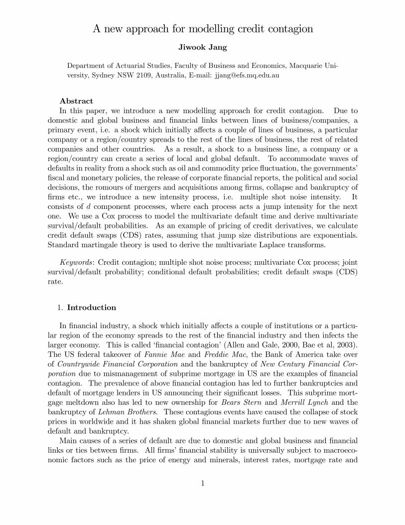
Proof. If we set �3 = �2 = �1 = 0 in (2.5) and (2.6) respectively, (2.7) and (2.9) follow. Ifwe also set �3 = �2 = �1 = 0 in (2.5) or set �3 = �2 = �1 = 1 in (2.6), (2.8) follows.

Corollary 2.5 The joint Laplace transform of the vector��(3)t ; �

(2)t ; �

(1)t

�where �(3)t ,

�(2)t and �

(1)t are jointly stationary is given by

Ene��1�

(1)t2 e��2�

(2)t2 e��3�

(3)t2

o= lim

t2�!1Ene��1�

(1)t2 e��2�

(2)t2 e��3�

(3)t2 j �(1)t1 ; �

(2)t1 ; �

(3)t1

o

= exp

2666666664��Z 1

0

26666666641� ^

g3

8>>>>>>>><>>>>>>>>:

�3e��(3)s

+e��(3)s

�R s0e�

(3)u

�

2641� ^g2

264 �2e��(2)u

+e��(2)u

�R u0e�

(2)wh1� ^

g1

h�1e

��(1)wiidw

375375 du

9>>>>>>>>=>>>>>>>>;

3777777775ds

3777777775:

(2.10)

Proof. Let t2 !1 in (2.8) and the result follows.

3. Joint/marginal survival probability and conditional default probabilities

9

Having derived the joint Laplace transform of the vector��(3)t ;�

(2)t ;�

(1)t

�; the joint

Laplace transform of the vector��(3)t ; �

(2)t ; �

(1)t

�and the joint p.g.f. of the vector

��(3)t ; �

(2)t ; �

(1)t

�in the previous section, we can easily calculate the joint/marginal survival probability andthe conditional default probabilities. Using (2.10), we have the joint Laplace transform of

the vector��(3)t ;�

(2)t ;�

(1)t

�where �(3)t , �

(2)t and �

(1)t are jointly stationary, i.e.

E

�e��3

n�(3)t2��(3)t1

oe��2

n�(2)t2��(2)t1

oe��1

n�(1)t2��(1)t1

o�= exp [�J(�3; �2; �1; t2;t1)]� exp [D(0; 0; 0; �3; �2; �1; 1; 1; 1; t2;t1)] ; (3.1)

where

J(�3; �2; �1; t2;t1) = ��

�Z 1

0

26666666666666666666666666666664

1� ^g3

8>>>>>>>>>>>>>>>>>>>>>>>>>>>>>><>>>>>>>>>>>>>>>>>>>>>>>>>>>>>>:

8>>>>><>>>>>:�3

�1�e��(3)(t2�t1)

�(3)

�+ e�

(3)t1 �R t2�t10

e��(3)(t2�s)

�

26641� ^g2

2664 �2

�1�e��(2)s

�(2)

�+ e��

(2)s

�R s0e�

(2)u

"1� ^

g1

(�1�(1)

� �1�(1)e��

(1)u

)#du

37753775 ds

9>>>>>=>>>>>;�e��(3)s

+e��(3)s �

R s0e�

(3)u

�

26666666666666641� ^

g2

8>>>>>>>>>>>>>><>>>>>>>>>>>>>>:

8>>>><>>>>:�2

�1�e��(2)(t2�t1)

�(2)

�+e��

(2)(t2�t1)R t2�t10

e�(2)s

�"1� ^

g1

(�1�(1)

� �1�(1)e��

(1)s

)#ds

9>>>>=>>>>; e��(2)u

+e��(2)u

�R u0e�

(2)w

2641� ^g1

8><>:(

�1�(1)

� �1�(1)e��

(1)(t2�t1)

)�e��(1)w

9>=>;375 dw

9>>>>>>>>>>>>>>=>>>>>>>>>>>>>>;

3777777777777775du

9>>>>>>>>>>>>>>>>>>>>>>>>>>>>>>=>>>>>>>>>>>>>>>>>>>>>>>>>>>>>>;

37777777777777777777777777777775

ds:

If we set �3 = �2 = �1 = 1 in (3.1), we can easily obtain the joint survival probability forwhich the stationary distribution of the default intensity is used, i.e.

E

�e�n�(3)t2��(3)t1

oe�n�(2)t2��(2)t1

oe�n�(1)t2��(1)t1

o�= exp [�J(1; 1; 1; t2;t1)]� exp [D(0; 0; 0; 1; 1; 1; 1; 1; 1; t2;t1)] : (3.2)

We omit the expressions for the joint default probability and other relevant joint probabilitiesas they can easily be obtained using (1.4), (1.5) and (3.2).To get the explicit expressions, now let us consider for i = 3; 2 and use an exponential

distribution of G(y(3)) and G(y(2)) for jump size respectively, i.e.

10

g(y(3)) = �e��y(3)

and g(y(2)) = �e��y(2)

with � > 0, � > 0;

then setting �3 = �2 = 1 and �1 = 0 in (3.1), the corresponding joint survival probability of�rm 3 and 2 is given by

E

�e�n�(3)t2��(3)t1

oe�n�(2)t2��(2)t1

o�

= exp

264��Z t2�t1

0

264�1�e��(3)s

�(3)

�+ e��

(3)sR s0e�

(3)zh

1�e��(2)z

��(2)+1�e��(2)z

idz

�+�1�e��(3)s

�(3)

�+ e��

(3)sR s0e�

(3)zh

1�e��(2)z��(2)+1�e��(2)z

idz

375 ds375

� exp

2666666666666666664

��Z 1

0

2666666666666666664

8><>:�1�e��(3)(t2�t1)

�(3)

�+e�

(3)t1R t2�t10

e��(3)(t2�u)

�1�e��(2)u

��(2)+�1�e��(2)u

��du

9>=>;� e��(3)s+e��

(3)sR s0e�

(3)z

� �1�e��(2)(t2�t1)

�e��

(2)z

��(2)+�1�e��(2)(t2�t1)

�e��

(2)z

�dz

�+

8><>:�1�e��(3)(t2�t1)

�(3)

�+e�

(3)t1R t2�t10

e��(3)(t2�u)

�1�e��(2)u

��(2)+�1�e��(2)u

��du

9>=>; e��(3)s+e��

(3)sR s0e�

(3)z

� �1�e��(2)(t2�t1)

�e��

(2)z

��(2)+�1�e��(2)(t2�t1)

�e��

(2)z

�dz

3777777777777777775

ds

3777777777777777775

:

(3.3)

Similarly, we can easily derive the corresponding joint survival probability of �rm 3 and 1,

i.e. E�e�n�(3)t2��(3)t1

oe�n�(1)t2��(1)t1

o�and the joint survival probability of �rm 2 and 1, i.e.

E

�e�n�(2)t2��(2)t1

oe�n�(1)t2��(1)t1

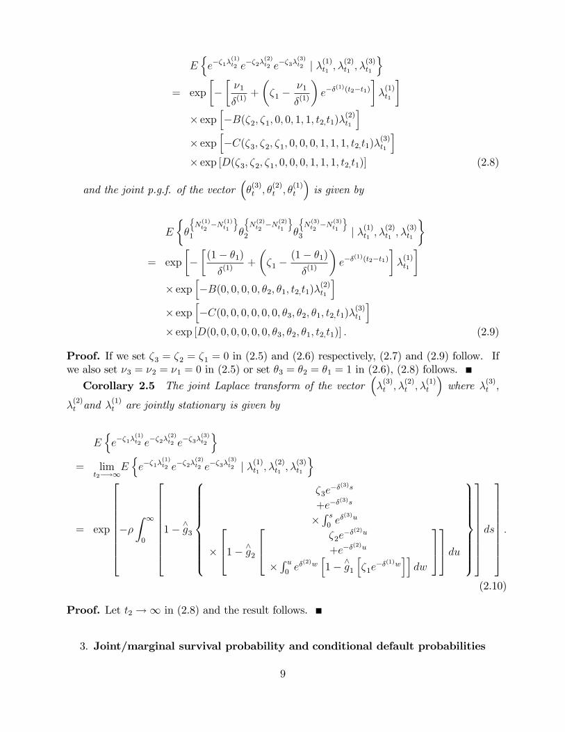
o�. If we set �2 = �1 = 0 and �3 = 1 in (3.1) and use an

exponential distribution for jump sizes, i.e. g(y(3)) = �e��y(3), then the survival probability

of �rm 3 which is the seeding company causing series of default, is given by

E

�e�n�(3)t2��(3)t1

o�=

8<: �e��(3)(t2�t1)

�+ 1

�(3)

�1� e��(3)(t2�t1)

�9=;

�

�(3)8<:�+

1

�(3)

�1� e��(3)(t2�t1)

��e��

(3)(t2�t1)

9=;��

�(3)�+1

;

(3.4)which can be found in Dassios and Jang (2003). If we set �3 = �1 = 0 and �2 = 1 in(3.1) and use an exponential distribution for jump sizes, i.e. g(y(2)) = �e��y

(2), the survival

probability of �rm 2 is given by

11

E

�e���(2)t2��(2)t1

��

= exp

2666666666664��Z 1

0

2666666666664

�e�

(3)t1R t2�t10

e��(3)(t2�u)

�1�e��(2)u

��(2)+�1�e��(2)u

��du

�e��

(3)s

+e��(3)sR s0e�

(3)z

� �1�e��(2)(t2�t1)

�e��

(2)z

��(2)+�1�e��(2)(t2�t1)

�e��

(2)z

�dz

�+

�e�

(3)t1R t2�t10

e��(3)(t2�u)

�1�e��(2)u

��(2)+�1�e��(2)u

��du

�e��

(3)s

+e��(3)sR s0e�

(3)z

� �1�e��(2)(t2�t1)

�e��

(2)z

��(2)+�1�e��(2)(t2�t1)

�e��

(2)z

�dz

3777777777775ds

3777777777775� exp

264��Z t2�t1

0

264 e��(3)sR s0e�

(3)zh

1�e��(2)z

��(2)+1�e��(2)z

idz

�+ e��(3)sR s0e�

(3)zh

1�e��(2)z��(2)+1�e��(2)z

idz

375 ds375 ; (3.5)

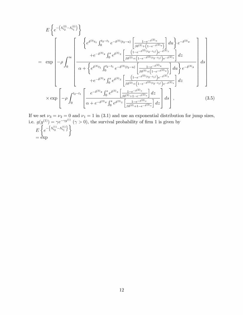
If we set �3 = �2 = 0 and �1 = 1 in (3.1) and use an exponential distribution for jump sizes,i.e. g(y(1)) = e� y

(1)( > 0), the survival probability of �rm 1 is given by

E

�e�n�(1)t2��(1)t1

o�= exp

12

0BBBBBBBBBBBBBBBBBBBBBBBBBBBBBBBBBBBBBBBBBBBBBBBBBBBBBBBBBBBBBB@

��

0BBBBBBBBBBBBBBBBBBBBBBBBBBBBBBBBBBBBBBBBBBBBBBBBBBBBBBBBBBBBBB@

R10

0BB@e�(3)t1 R t2�t10e��

(3)(t2�s)

0BB@ e��(2)s

R s0 e

�(2)u

0@ 1�e��(1)u

�(1)+

�1�e��(1)u

�1Adu

�+e��(2)s

R s0 e

�(2)u

0@ 1�e��(1)u

�(1)+

�1�e��(1)u

�1Adu

1CCA ds1CCA

�e��(3)s+e��

(3)sR s0e�

(3)u

�

0BBBBBBBBBBB@

�e��

(2)(t2�t1)R t2�t10

e�(2)s

�1�e��(1)s

�(1)+�1�e��(1)s

��ds

�� e��(2)u

+e��(2)uR u0e�

(2)w

� �1�e��(1)(t2�t1)

�e��

(1)w

�(1)+�1�e��(1)(t2�t1)

�e��

(1)w

�dw

� +

�e��

(2)(t2�t1)R t2�t10

e�(2)s

�1�e��(1)s

�(1)+�1�e��(1)s

��ds

�� e��(2)u

+e��(2)uR u0e�

(2)w

� �1�e��(1)(t2�t1)

�e��

(1)w

�(1)+�1�e��(1)(t2�t1)

�e��

(1)w

�dw

1CCCCCCCCCCCAdu

�+

0BB@e�(3)t1 R t2�t10e��

(3)(t2�s)

0BB@ e��(2)s

R s0 e

�(2)u

0@ 1�e��(1)u

�(1)+

�1�e��(1)u

�1Adu

�+e��(2)s

R s0 e

�(2)u

0@ 1�e��(1)u

�(1)+

�1�e��(1)u

�1Adu

1CCA ds1CCA

�e��(3)s+e��

(3)sR s0e�

(3)u

�

0BBBBBBBBBBBBBBB@

�e��

(2)(t2�t1)R t2�t10

e�(2)s

�1�e��(1)s

�(1)+�1�e��(1)s

��ds

��e��(2)u

+e��(2)uR u0e�

(2)w

� �1�e��(1)(t2�t1)

�e��

(1)w

�(1)+�1�e��(1)(t2�t1)

�e��

(1)w

�dw

� +

�e��

(2)(t2�t1)R t2�t10

e�(2)s

�1�e��(1)s

�(1)+�1�e��(1)s

��ds

�� e��(2)u

+e��(2)uR u0e�

(2)w

� �1�e��(1)(t2�t1)

�e��

(1)w

�(1)+�1�e��(1)(t2�t1)

�e��

(1)w

�dw

1CCCCCCCCCCCCCCCAdu

1CCCCCCCCCCCCCCCCCCCCCCCCCCCCCCCCCCCCCCCCCCCCCCCCCCCCCCCCCCCCCCA

ds

1CCCCCCCCCCCCCCCCCCCCCCCCCCCCCCCCCCCCCCCCCCCCCCCCCCCCCCCCCCCCCCA

� exp

0BBBBBBBBBBB@��Z t2�t1

0

0BBBBBBBBBBB@

e��(3)sR s0e�

(3)u �

0BB@ e��(2)u

R u0 e

�(2)w

0@ 1�e��(1)w

�(1)+

�1�e��(1)w

�1Adw

�+e��(2)u

R u0 e

�(2)w

0@ 1�e��(1)w

�(1)+

�1�e��(1)w

�1Adw

1CCA du

�+ e��(3)sR s0e�

(3)u �

0BB@ e��(2)u

R u0 e

�(2)w

0@ 1�e��(1)w

�(1)+

�1�e��(1)w

�1Adw

�+e��(2)u

R u0 e

�(2)w

0@ 1�e��(1)w

�(1)+

�1�e��(1)w

�1Adw

1CCA du

1CCCCCCCCCCCAds

1CCCCCCCCCCCA:

(3.6)

Using Bayes�rule, the conditional default probabilities between �rm 3 and 2, denoted by

13

p3j2 and p2j3 can be calculated by

p3j2 =p32p2=Pr (� 3 � t; � 2 � t)

Pr (� 2 � t)

=1� E

ne��

(3)t

o� E

ne��

(2)t

o+ E

ne��

(3)t e��

(2)t

o1� E

ne��

(2)t

o ;

p2j3 =p32p3=Pr (� 3 � t; � 2 � t)

Pr (� 3 � t)

=1� E

ne��

(3)t

o� E

ne��

(2)t

o+ E

ne��

(3)t e��

(2)t

o1� E

ne��

(3)t

oand other conditional default probabilities can be easily driven using (3.2).Now let us illustrate the calculations of the joint survival/default probabilities, relevant

joint probabilities and the conditional default probabilities.Example 3.1We assume that the magnitude of the contribution to the default intensity of the �rm 3

from the primary events is higher than that of the �rm 2. We also assume that the decay ratefor the �rm 3, that measures how quick the �rm gets out of the in�uence of primary eventslowering their default intensity rate, is lower than that for the �rm 2. So the parametervalues used to calculate the joint probabilities are

� = 5; � = 10; �(3) = 0:3, �(2) = 0:5 and � = 4:

Setting t1 = 0 and t2 = 1; joint survival probability is given by

Pr (� 3 > 1; � 2 > 1) = Ene��

(3)1 e��

(2)1

oand relevant joint probabilities are given by

Pr (� 3 � 1; � 2 > 1) = Ene��

(2)1

o� E

ne��

(3)1 e��

(2)1

oPr (� 3 > 1; � 2 � 1) = E

ne��

(3)1

o� E

ne��

(3)1 e��

(2)1

o,

and the joint default probability is given by

Pr (� 3 � 1; � 2 � 1) = 1� Ene��

(3)1

o� E

ne��

(2)1

o+ E

ne��

(3)1 e��

(2)1

o:

From the equation (3.3)-(3.5), the calculations of the joint survival/default probability,relevant joint probabilities and the conditional default probability are given by

14

Pr (� 3 > 1; � 2 > 1) = 0:05492

Pr (� 3 � 1; � 2 > 1) = 0:54808;

Pr (� 3 > 1; � 2 � 1) = 0:03137;

Pr (� 3 � 1; � 2 � 1) = 0:36563 (3.7)

and

p3j2 = 0:92098 and p2j3 = 0:40016; (3.8)

where

Pr (� 3 > 1) = 0:08629 and Pr (� 2 > 1) = 0:603; (3.9)

Pr (� 3 � 1) = 0:91371 and Pr (� 2 � 1) = 0:397. (3.10)

The joint survival probability is given by 0:05492 which is much lower than the survivalprobability of the �rm 2, 0:603 and lower than the survival probability of the �rm 3, 0:08629.The joint probabilities where the survivorship of the �rm 2 is concerned are determined bythe survival or default probability of the �rm 3, i.e. as the default probability of the �rm 3is higher than its survival probability we have

Pr (� 3 � 1; � 2 > 1) = 0:54808 > Pr (� 3 > 1; � 2 > 1) = 0:05492:

Similarly, the joint default probability is given by 0:36563 which is much lower than thedefault probability of the �rm 3, 0:91371 and lower than the default probability of the �rm2, 0:397. The joint probabilities where the defaultability of the �rm 2 is concerned aredetermined by the survival or default probability of the �rm 3, i.e. as the default probabilityof the �rm 3 is higher than its survival probability we have

Pr (� 3 � 1; � 2 � 1) = 0:36563 > Pr (� 3 > 1; � 2 � 1) = 0:03137:The conditional default probabilities are rescaled to the joint default probability by the

default probability of the �rm 3 and 2 in (3.10) respectively. Hence the default probabilitiesof the �rm 3 (or 2) given that the �rm 2 (or 3) defaults in (3.8) are very similar to theunconditional default probability of the �rm 3 (or 2) in (3.10).Next examples shows that the calculations of the joint survival/default probability, rel-

evant joint probabilities and the conditional default probability by changing the values ofthe jump frequency rate �, the values of the magnitude of jump size � and the values ofexponential decay �(3) respectively.Example 3.2Using the same parameter values used in Example 3.1 except for � = 10; � = 1 and �(3) =

0:01, the calculations of the joint survival/default probability, relevant joint probabilities andthe conditional default probability are given in Table 3.1.

15

Table 3.1.� = 10 � = 1 �(3) = 0:01

Pr (� 3 > 1; � 2 > 1)= 0:00070684

Pr (� 3 > 1; � 2 > 1)= 0:000016267

Pr (� 3 > 1; � 2 > 1)= 0

Pr (� 3 � 1; � 2 > 1)= 0:2816532

Pr (� 3 � 1; � 2 > 1)= 0:089082733

Pr (� 3 � 1; � 2 > 1)= 0

Pr (� 3 > 1; � 2 � 1)= 0:0014804

Pr (� 3 > 1; � 2 � 1)= 0:000061367

Pr (� 3 > 1; � 2 � 1)= 0

Pr (� 3 � 1; � 2 � 1)= 0:7161596

Pr (� 3 � 1; � 2 � 1)= 0:910839633

Pr (� 3 � 1; � 2 � 1)= 1

p3j2 = 0:99794and p2j3 = 0:71773

p3j2 = 0:99993and p2j3 = 0:91091

p3j2 = 1and p2j3 = 1

Pr (� 3 > 1) = 0:0021872and Pr (� 2 > 1) = 0:28236

Pr (� 3 > 1) = 0:000077634and Pr (� 2 > 1) = 0:089099

Pr (� 3 > 1) = 0and Pr (� 2 > 1) = 0

Pr (� 3 � 1) = 0:9978128and Pr (� 2 � 1) = 0:71764

Pr (� 3 � 1) = 0:999922366and Pr (� 2 � 1) = 0:910901

Pr (� 3 � 1) = 1and Pr (� 2 � 1) = 1

Firstly, Table 3.1 shows that the higher the jump arrival rate in �rm 3 default intensity�(3)t ; � is, i.e. the more frequent arrival of primary events is, the joint/marginal survivalprobabilities are getting closer to 0. Secondly it shows that the lower � is, i.e. the biggerthe magnitude of the contribution to the default intensity of the �rm 3 from the primaryevents is, the joint/marginal survival probabilities are getting closer to 0. Lastly we can seethat the lower �(3) is, i.e. the slower the �rm gets out of the in�uence of primary events, thejoint/marginal survival probabilities are getting closer to 0.We omit the corresponding calculations for the joint survival/default probability, relevant

joint probabilities and the conditional default probability by changing the values of themagnitude of jump size � and the values of exponential decay �(2) as they can be easilyobtained. It is obvious that the lower � and the lower �(3) is, the joint/marginal survivalprobabilities are getting closer to 0.

4. Measuring credit default swaps (CDS) rate

In this Section, we apply the results in Section 3 in pricing of a �nancial product For thatpurpose, we choose credit default swaps (CDS) as three parties are involved in this contract,i.e. a reference credit, a CDS buyer and a CDS seller. In order to calculate credit defaultswaps (CDS) rate, �rstly we assume that deterministic instantaneous rate of interest r for azero-coupon default-free bond. Then its price at time 0, paying 1 at time t is given by

B(0; t) = e�rt; (4.1)

where B(0; t) denotes the price of a default-free zero-coupon bond.Now we denote the default intensity process of a CDS buyer and seller by �(b)t and �(s)t ,

respectively. We also specify the default intensity process of a reference credit by �(rc)t . Forsimplicity, we assume a deterministic recovery rate �. Then credit default swaps (CDS)

16

rate, denoted by s, is given by

s = (1� �)

kNPk=1

erc;s(0; tk�1; tk)

NPn=1

(tkn+1 � tkn)Bb(0; tkn)

; (4.2)

where

erc;s(0; tk�1; tk)

= E

26664exp

��

tkR0

rsds

�(exp

�

tk�1R0

�(rc)s ds

!� exp

��

tkR0

�(rc)s ds

�)��exp

��

tkR0

�(s)s ds

��j �(rc)0 ; �

(s)0

37775 ;(4.3)

Bb(0; tkn) = E

24exp8<:�

tknZ0

�rs + �

(b)s

�ds

9=; j �(b)0

35 (4.4)

and tk1 < tk2 < � � � < tkn. Assuming that �(i)t is stationary, the equation (4.3) and (4.4) can

be expressed as

erc;s(0; tk�1; tk)

= e�rtk �

24E�e��(rc)tk�1e��(s)tk�1

�E

8<:exp0@� tkZ

tk�1

�(s)s ds

1A9=;� E�e��(rc)tk e��(s)tk

�35= e�rtk �

�E�e��(rc)tk�1e

��(s)tk�1

�E�e���(s)tk��(s)tk�1

��� E

�e��

(rc)tk e��

(s)tk

��(4.5)

and

Bb(0; tkn) = e

�rtknE�e��(b)tkn

�: (4.6)

Using the equation (4.6), we may consider pricing defaultable bonds as well as credit spreadbetween default-free bond and defaultable bond. Also based on the results in Section 2and 3, i.e. using multiple shot noise intensity, we can calculate the joint survival probabilitybetween the reference credit and CDS seller and the survival probability of CDS buyer invarious ways.Now to illustrate the calculations of credit default swaps (CDS) rates, let us assume that

the default intensity process of reference credit follows �(3)t with �; �(rc) and �(rc), i.e.

�(3)t = �

(rc)t with �; �(rc) and �(rc)

17

and that the default intensity process of CDS seller follows �(2)t with �(s) and �(s), i.e.

�(2)t = �

(s)t with �(s) and �(s)

and that the default intensity process of CDS buyer follows �(2)t with �(b) and �(b); i.e.

�(2)t = �

(b)t with �(b) and �(b):

The above assumptions mean that �rstly the default intensity of a CDS seller and of a CDSbuyer are contaminated by the default intensity of a reference credit which is the seedingcompany, respectively. Secondly, the defaultability (or survivorship) of a reference creditand the defaultability (or survivorship) of a CDS seller are jointly related and they are notindependent each other. Also the defaultability (or survivorship) of a reference credit andthe defaultability (or survivorship) of a CDS buyer are dependent each other.Example 4.1We assume that the magnitude of the contribution to the default intensity of a reference

credit from the primary events is bigger than the magnitude of a CDS seller�s default intensityand of a CDS buyer�s intensity, respectively. The magnitude of a CDS seller�s defaultintensity is bigger than that of a CDS buyer�s intensity. It is also assumed that the decayrate in a reference credit�s intensity, that measures how quick a reference credit gets out ofthe in�uence of primary events lowering its default intensity rate, is lower than the decayrate in a CDS seller�s intensity and the decay rate in a CDS buyer�s intensity, respectively.The decay rate in a CDS seller�s intensity is lower than that of in a CDS buyer�s intensity.So the parameter values used to calculate (4.2) are

�(rc) = 5; �(s) = 10; �(b) = 20; �(rc) = 0:3, �(s) = 0:5; �(b) = 1 and � = 4: (4.7)

and

r = 0:05; � = 50%, N = 2; tk0 = 0; tk1 = 0:5 and tk2 = 1: (4.8)

For E�e��

(rc)t e��

(s)t

�in (4.5) and for E

�e��

(b)t

�in (4.6), (3.3) and (3.5) are used respectively,

for which using the same parameter values above, the calculations of credit default swaps(CDS) rates by changing in the values of �, �(rc) and �(rc) for a reference credit are shownin Table 4.1-4.3.

Table 4.1.

s� = 50 18:364bp� = 30 175:31bp� = 10 1633:2bp� = 4 3126:2bp� = 1 2809:9bp

Table 4.2.

s

�(rc) = 1 606:53bp�(rc) = 5 3126:2bp�(rc) = 10 3515:6bp�(rc) = 15 3290:0bp�(rc) = 20 2964:3bp

Table 4.3.

s

�(rc) = 0:01 0:01699bp�(rc) = 0:1 1407:9bp�(rc) = 0:3 3126:2bp�(rc) = 0:5 3064:2bp�(rc) = 1 1886:5bp

In Table 4.1, �rstly we can see that if the primary event arrival rate � is getting higher,the credit swap rate is getting higher. It is obvious as a CDS seller should charge higher

18

rate when the primary event arrivals are more frequent. However the credit swap rate startsdecreasing due to contagion. It happens as the higher the primary event arrival rate, � is,the more likely for a reference credit to default and the higher the jump arrival rate of �(rc)t

for a credit swap seller and for a credit swap buyer, respectively. As a result, a credit swapseller�s default intensity is getting higher and its increase is much bigger than the increase ofcredit swap buyer�s default intensity due to the parameter values used in (4.7). Eventuallyit may lead to a credit swap seller�s default which happens quicker than a credit swap buyer�sdefault. The credit swap rates are getting lower as a credit swap seller�s default intensity isgetting higher due to higher the jump arrival rate of �(rc)t for a credit swap seller.Secondly, Table 4.2 shows that if the magnitude of contribution of primary event i to

intensity �(rc)t is getting higher (i.e. the lower �(rc) value is), the credit swap rate is gettinghigher as the more likely for the reference credit to default. However similar to Table 4.1,the credit swap rate is getting lower due to contagion. It is as the lower �(rc) value is, themore likely for a reference credit to default and the higher the jump arrival rate of �(rc)t fora credit swap seller and for a credit swap buyer, respectively. The swap rates decreases asa credit swap seller�s default intensity is getting higher due to higher the jump arrival rateof �(rc)t for a credit swap seller.Lastly, it is shown that the slower a reference credit gets out of the in�uence from primary

events (i.e. the lower �(rc) value is), the credit swap fee is getting higher in Table 4.3. Howeversimilar to Table 4.1-4.2, the credit swap fee decreases due to contagion. It happens as thelower �(rc) value is, the more likely for a reference credit to default and the higher the jumparrival rate of �(rc)t for a credit swap seller and for a credit swap buyer, respectively. Theswap rates are getting lower as a credit swap seller no longer able to guarantee the paymentto a credit swap buyer due to a credit swap seller�s high default intensity.Let us now examine the e¤ect on credit default swaps (CDS) rate caused by changes in

the value of �(s) and �(s) for a CDS seller.Example 4.2Using the same parameter values of (4.7) and (4.8), the calculations of credit default

swaps (CDS) rates caused by changes in the value of �(s) and �(s) for a CDS seller are shownin Table 4.4 and Table 4.5, respectively.

Table 4.4.

s

�(s) = 1 125:71bp�(s) = 5 1921:2bp�(s) = 10 3126:2bp�(s) = 15 3719:2bp�(s) = 20 4066:1bp

Table 4.5.

s

�(s) = 0:01 0bp�(s) = 0:1 428:53bp�(s) = 0:3 2238:0bp�(s) = 0:5 3126:2bp�(s) = 1 4034:7bp

Table 4.4 and 4.5 show that CDS rate is getting lower to 0 by decreasing the value of �(s)

and �(s) for the CDS seller. It is as the lower �(s) value and the lower �(s) value is respectively,the more likely the CDS seller defaults and the lower CDS rate becomes. Hence it is gettingcheaper for a CDS buyer to purchase a CDS contract, however a CDS buyer should bear inmind that the lower the CDS rate is, the more likely a CDS seller defaults. The worst casescenario for a CDS buyer is when both a reference credit and a CDS seller default.

19

The next example examines the e¤ect on credit default swaps (CDS) rate caused bychanges in the value of �(b) and �(b) for a CDS buyer.Example 4.3Using the same parameter values of (4.7) and (4.8), the calculations of credit default

swaps (CDS) rates caused by changes in the value of �(b) and �(b) for a CDS buyer are shownin Table 4.6 and Table 4.7, respectively.

Table 4.6.

s

�(b) = 5 4081:4bp�(b) = 10 3430:2bp�(b) = 15 3225:9bp�(b) = 20 3126:2bp

Table 4.7.

s

�(b) = 0:1 7101:2bp�(b) = 0:3 3898:5bp�(b) = 0:5 3439:2bp�(b) = 1 3126:2bp

Table 4.6 and 4.7 show that CDS rate is getting higher by decreasing the value of �(b) and�(b) for the CDS buyer. It is as the lower �(b) value and the lower �(b) value is respectively,the more likely the CDS buyer defaults and the higher CDS rate becomes. Hence the feepayments made by a CDS buyer to a CDS seller is getting higher, however a CDS sellershould bear in mind that the higher the CDS rate is, the more likely a CDS buyer defaults.A worst case scenario for a CDS seller is when a CDS buyer defaults soon after a CDScontract is initiated as there are no more fee payments made by a CDS buyer.

5. Conclusion

We used multiple shot noise default intensity, where each process acts a jump intensityfor the next one, to model credit contagion. Using a Cox process to model the multivariatedefault time with the assumption that default jumps, intensity jumps and primary eventjumps are independent of each other and standard martingale theory, the expressions for thejoint/marginal survival probability and conditional default probabilities and their calcula-tions were shown. For the application of these expressions, the calculations of credit defaultswaps (CDS) rates ware presented as three parties are involved in this contract where weused exponential distributions for jump sizes. We also examined the relationship betweenCDS rates and the parameter values in default intensity for the reference credit, for the CDSseller and for CDS buyer respectively.Neither linear correlation nor copula-based non-linear correlation used in this paper.

On the contrary, we used multivariate intensity-based framework, i.e. a multivariate Coxprocess with multiple shot noise intensity to accommodate counterparty risks and to priceCDS considering credit contagion from primary events. We leave the pricing of creditportfolio derivatives such as CDOs for further research based on our modeling approach.

References

Allen F. and Gale, D. (2000): Financial Contagion, Journal of Political Economy,108/1, 1-34.

20

Bae, K.-H., Karolyi, G. A. and Stulz, R. M. M. (2003): A New Approach toMeasuring Financial Contagion, The Review of Financial Studies, 16/3, 717-763.

Brémaud, P. (1981): Point Processes and Queues: Martingale Dynamics, Springer-Verlag, New-York.

Cox, D. R. (1955): Some statistical methods connected with series of events, J.R. Stat. Soc. B, 17, 129-164.

Dassios, A. (1987): Insurance, Storage and Point Process: An Approach viaPiecewise Deterministic Markov Processes, Ph.D. Thesis, Imperial College, Lon-don.

Dassios, A. and Jang, J. (2003): Pricing of catastrophe reinsurance & derivativesusing the Cox process with shot noise intensity, Finance & Stochastics, 7/1, 73-95.

Dassios, A. and Sculli, P. (2008): Contagion in A¢ ne Default Processes, Pro-ceedings of the 2008 Forum of IEF.

Eglo¤a, D., Leippold, M. and Vanini, P. (2007): A simple model of credit conta-gion, Journal of Banking and Finance, 31/8, 2475-2492.

Frey, R. and Backhaus, J. (2008): Pricing and Hedging of Portfolio Credit Deriv-atives with Interacting Default Intensities, International Journal of Theoreticaland Applied Finance, 11/6, 611-634.

Giesecke, K. and Weber, S. (2004): Cyclical correlations, credit contagion, andportfolio losses, Journal of Banking and Finance, 28/12, 3009�3036.

Giesecke, K. andWeber, S. (2006): Credit contagion and aggregate losses, Journalof Economic Dynamics and Control, 30, 741-767.

Grandell, J. (1976) : Doubly Stochastic Poisson Processes, Springer-Verlag, Berlin.

Herbertsson, A. and Rootzén, H. (2008): Pricing kth-to-default swaps under de-fault contagion: the matrix analytic approach, Journal of Computational Finance,12/1.

Leung, K. S.and Kwok, Y. K. (2007): Contagion models with interacting de-fault intensity processes, Proceedings of the International Congress of ChineseMathematicians, Vol. III, 748-758.

Schönbucher, P. J. (2003): Information-driven default contagion, Working paper.ETH Zurich.

21