Central Idaho (CI) Variant Overview - US Forest Service Central Idaho (CI) Variant Overview Forest...

United States Department of Agriculture

Forest Service

Forest Management Service Center

Fort Collins, CO

2008

Revised:

November 2015

Central Idaho (CI) Variant Overview

Forest Vegetation Simulator

Douglas-fir forest in Little West Fork, Salmon-Challis National Forest

(Sharon Skroh Bradley, FS-R4)

iii

Central Idaho (CI) Variant Overview

Forest Vegetation Simulator

Compiled By:

Chad E. Keyser USDA Forest Service Forest Management Service Center 2150 Centre Ave., Bldg A, Ste 341a Fort Collins, CO 80526 Gary E. Dixon Management and Engineering Technologies, International Forest Management Service Center 2150 Centre Ave., Bldg A, Ste 341a Fort Collins, CO 80526

Authors and Contributors:

The FVS staff has maintained model documentation for this variant in the form of a variant overview since its release in 1988. The original author was Gary Dixon. In 2008, the previous document was replaced with this updated variant overview. Gary Dixon, Christopher Dixon, Robert Havis, Chad Keyser, Stephanie Rebain, Erin Smith-Mateja, and Don Vandendriesche were involved with this major update. Don Vandendriesche cross-checked information contained in this variant overview with the FVS source code. The species list for this variant was expanded and this document was extensively revised by Gary Dixon in 2011. Current maintenance is provided by Chad Keyser.

Keyser, Chad E.; Dixon, Gary E., comp. 2008 (revised November 2, 2015). Central Idaho (CI) Variant Overview – Forest Vegetation Simulator. Internal Rep. Fort Collins, CO: U. S. Department of Agriculture, Forest Service, Forest Management Service Center. 52p.

iv

Table of Contents

1.0 Introduction ................................................................................................................................ 1

2.0 Geographic Range ....................................................................................................................... 2

3.0 Control Variables ........................................................................................................................ 3

3.1 Location Codes .................................................................................................................................................................. 3

3.2 Species Codes .................................................................................................................................................................... 3

3.3 Habitat Type, Plant Association, and Ecological Unit Codes ............................................................................................. 4

3.4 Site Index ........................................................................................................................................................................... 4

3.5 Maximum Density ............................................................................................................................................................. 6

4.0 Growth Relationships .................................................................................................................. 7

4.1 Height-Diameter Relationships ......................................................................................................................................... 7

4.2 Bark Ratio Relationships .................................................................................................................................................... 8

4.3 Crown Ratio Relationships ................................................................................................................................................ 9

4.3.1 Crown Ratio Dubbing............................................................................................................................................... 10

4.3.2 Crown Ratio Change ................................................................................................................................................ 13

4.3.3 Crown Ratio for Newly Established Trees ............................................................................................................... 13

4.4 Crown Width Relationships ............................................................................................................................................. 13

4.5 Crown Competition Factor .............................................................................................................................................. 15

4.6 Small Tree Growth Relationships .................................................................................................................................... 17

4.6.1 Small Tree Height Growth ....................................................................................................................................... 17

4.6.2 Small Tree Diameter Growth ................................................................................................................................... 21

4.7 Large Tree Growth Relationships .................................................................................................................................... 23

4.7.1 Large Tree Diameter Growth ................................................................................................................................... 23

4.7.2 Large Tree Height Growth ....................................................................................................................................... 30

5.0 Mortality Model ....................................................................................................................... 34

6.0 Regeneration ............................................................................................................................ 38

7.0 Volume ..................................................................................................................................... 41

8.0 Fire and Fuels Extension (FFE-FVS) ............................................................................................. 43

9.0 Insect and Disease Extensions ................................................................................................... 43

10.0 Literature Cited ....................................................................................................................... 44

11.0 Appendices ............................................................................................................................. 47

11.1 Appendix A. Habitat Codes ............................................................................................................................................ 47

v

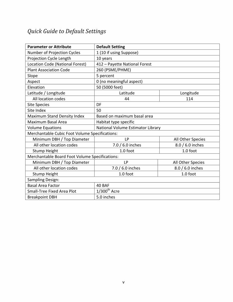
Quick Guide to Default Settings

Parameter or Attribute Default Setting Number of Projection Cycles 1 (10 if using Suppose) Projection Cycle Length 10 years Location Code (National Forest) 412 – Payette National Forest Plant Association Code 260 (PSME/PHME) Slope 5 percent Aspect 0 (no meaningful aspect) Elevation 50 (5000 feet) Latitude / Longitude Latitude Longitude All location codes 44 114 Site Species DF Site Index 50 Maximum Stand Density Index Based on maximum basal area Maximum Basal Area Habitat type specific Volume Equations National Volume Estimator Library Merchantable Cubic Foot Volume Specifications: Minimum DBH / Top Diameter LP All Other Species All other location codes 7.0 / 6.0 inches 8.0 / 6.0 inches Stump Height 1.0 foot 1.0 foot Merchantable Board Foot Volume Specifications: Minimum DBH / Top Diameter LP All Other Species All other location codes 7.0 / 6.0 inches 8.0 / 6.0 inches Stump Height 1.0 foot 1.0 foot Sampling Design: Basal Area Factor 40 BAF Small-Tree Fixed Area Plot 1/300th Acre Breakpoint DBH 5.0 inches

1

1.0 Introduction

The Forest Vegetation Simulator (FVS) is an individual tree, distance independent growth and yield model with linkable modules called extensions, which simulate various insect and pathogen impacts, fire effects, fuel loading, snag dynamics, and development of understory tree vegetation. FVS can simulate a wide variety of forest types, stand structures, and pure or mixed species stands.

New “variants” of the FVS model are created by imbedding new tree growth, mortality, and volume equations for a particular geographic area into the FVS framework. Geographic variants of FVS have been developed for most of the forested lands in United States.

The Central Idaho (CI) variant had an interesting development history. The University of Idaho originally developed a CI variant in 1982. This variant was used in Region 4 for several years, but it was not part of the FVS suite of software tools. Model maintenance was problematic for the developers and the growth relationships themselves did not produce reliable results.

In February 1988 the University of Idaho completed work on new large tree diameter increment models for six major commercial species. In July 1988, Region 4 requested the Forest Management Service Center develop a new CI variant using the newly developed large tree diameter models from the University of Idaho, height and crown models from the Northern Idaho (NI) variant, and the mortality model from the Teton (TT) variant. So the true CI variant, as a part of the FVS system, was released in late 1988.

Since the variant’s completion in 1988, many of the functions have been adjusted and improved as more data has become available and as model technology has advanced. In 2011 this variant was expanded from 11 species to 19 species. Species added include whitebark pine, Pacific yew, quaking aspen, western juniper, curlleaf mountain-mahogany, limber pine, and black cottonwood. The “other species” grouping was split into other softwoods and other hardwoods. Whitebark pine, limber pine, and Pacific yew use whitebark/limber pine equations from the Tetons variant; quaking aspen uses aspen equations from the Utah variant; western juniper uses western juniper equations from the Utah variant; curlleaf mountain-mahogany uses other hardwoods equations from the Westside Cascades variant as implemented for curlleaf mountain-mahogany in the Utah variant; black cottonwood and other hardwoods use cottonwood equations from the Central Rockies variant as implemented for other hardwoods in the Inland Empire variant; and other softwoods uses the equations for the original other species grouping in the 11 species version of this variant.

To fully understand how to use this variant, users should also consult the following publication:

• Essential FVS: A User’s Guide to the Forest Vegetation Simulator (Dixon 2002)

This publication can be downloaded from the Forest Management Service Center (FMSC), Forest Service website or obtained in hard copy by contacting any FMSC FVS staff member. Other FVS publications may be needed if one is using an extension that simulates the effects of fire, insects, or diseases.

2

2.0 Geographic Range

The CI variant was fit to data representing forest types in central Idaho. Data used in model development came from forest inventories on the Boise, Challis, Payette, Salmon, and Sawtooth National Forests.

The CI variant covers forest types in Central Idaho. The suggested geographic range of use for the CI variant is shown in figure 2.0.1.

Figure 2.0.1 Suggested geographic range of use for the CI variant.

3

3.0 Control Variables

FVS users need to specify certain variables used by the CI variant to control a simulation. These are entered in parameter fields on various FVS keywords usually brought into the simulation through the SUPPOSE interface data files or they are read from an auxiliary database using the Database Extension.

3.1 Location Codes

The location code is a 3-digit code where, in general, the first digit of the code represents the USDA Forest Service Region Number, and the last two digits represent the Forest Number within that region.

If the location code is missing or incorrect in the CI variant, a default forest code of 412 (Payette National Forest) will be used. A complete list of location codes recognized in the CI variant is shown in table 3.1.1.

Table 3.1.1 Location codes used in the CI variant.

Location Code USFS National Forest 117 Nez Perce 402 Boise 406 Challis 412 Payette 413 Salmon 414 Sawtooth

3.2 Species Codes

The CI variant recognizes 17 individual species along with other softwoods and other hardwoods species groupings. You may use FVS species codes, Forest Inventory and Analysis (FIA) species codes, or USDA Natural Resources Conservation Service PLANTS symbols to represent these species in FVS input data. Any valid western species codes identifying species not recognized by the variant will be mapped to the most similar species in the variant. The species mapping crosswalk is available on the variant documentation webpage of the FVS website. Any non-valid species code will default to the “other hardwoods” category.

Either the FVS sequence number or alpha code must be used to specify a species in FVS keywords and Event Monitor functions. FIA codes or PLANTS symbols are only recognized during data input, and may not be used in FVS keywords. Table 3.2.1 shows the complete list of species codes recognized by the CI variant.

Table 3.2.1 Species codes used in the CI variant.

Species Number

Species Code Common Name FIA

Code PLANTS Symbol Scientific Name

1 WP western white pine 119 PIMO3 Pinus monticola 2 WL western larch 73 LAOC Larix occidentalis 3 DF Douglas-fir 202 PSME Pseudotsuga menziesii

4

Species Number

Species Code Common Name FIA

Code PLANTS Symbol Scientific Name

4 GF grand fir 17 ABGR Abies grandis 5 WH western hemlock 263 TSHE Tsuga heterophylla 6 RC western redcedar 242 THPL Thuja plicata 7 LP lodgepole pine 108 PICO Pinus contorta 8 ES Engelmann spruce 93 PIEN Picea engelmannii 9 AF subalpine fir 19 ABLA Abies lasiocarpa

10 PP ponderosa pine 122 PIPO Pinus ponderosa 11 WB whitebark pine 101 PIAL Pinus albicaulis 12 PY Pacific yew 231 TABR2 Taxus brevifolia 13 AS quaking aspen 746 POTR5 Populus tremuloides 14 WJ western juniper 64 JUOC Juniperus occidentalis

15 MC curlleaf mountain-mahogany 475 CELE3 Cercocarpus ledifolius

16 LM limber pine 113 PIFL2 Pinus flexilis

17 CW black cottonwood 747 POBAT Populus balsamifera var. trichocarpa

18 OS other softwoods 298 2TE 19 OH other hardwoods 998 2TD

3.3 Habitat Type, Plant Association, and Ecological Unit Codes

There are 130 habitat type codes recognized in the CI variant. If the habitat type code is blank or not recognized, the default 260 (PSME/PHMA) will be assigned. The 130 habitat type codes are mapped to one of the 30 original North Idaho (NI) variant habitat type codes. A list of valid CI variant’s habitat type codes and the original NI habitat type code equivalents can be found in table 11.1.1 of Appendix A.

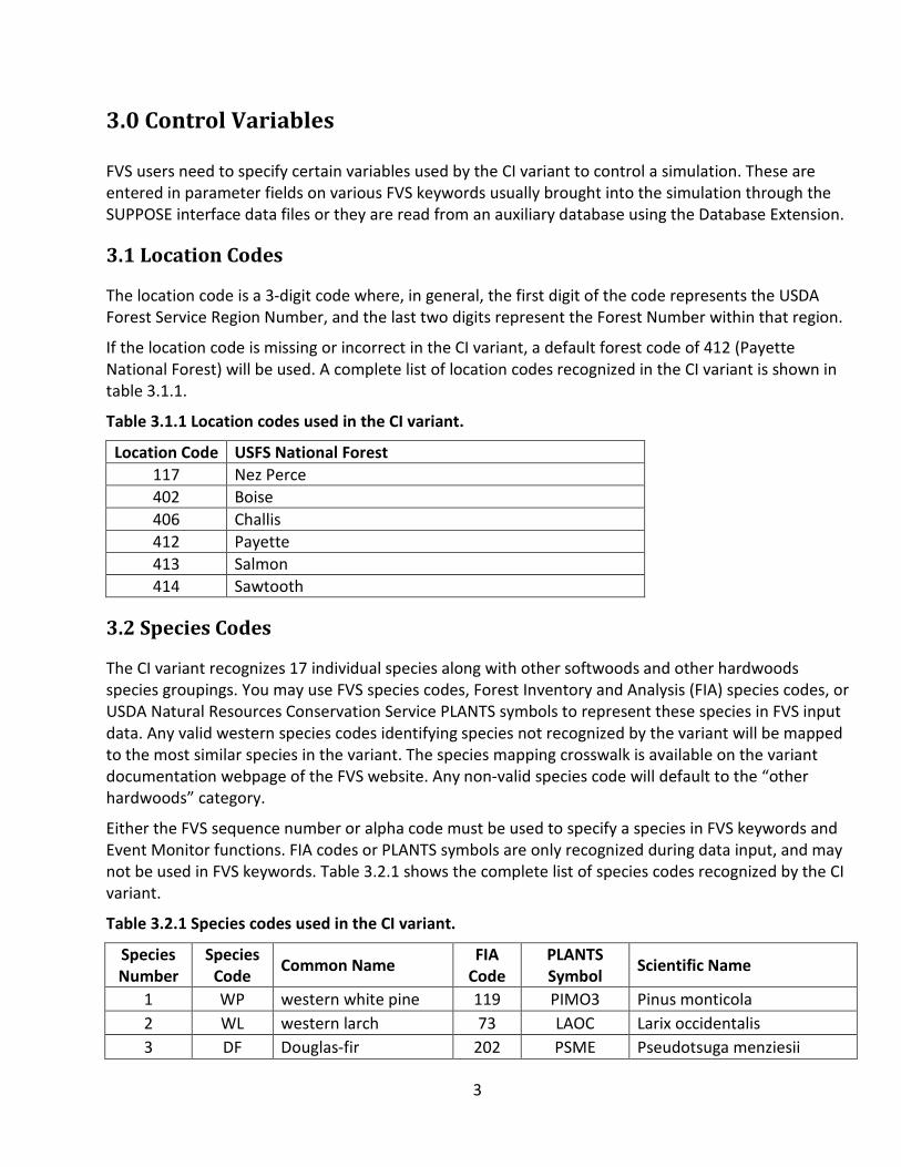
3.4 Site Index

Site index is used in equations for some species in the CI variant. These species are whitebark pine, Pacific yew, quaking aspen, western juniper, curlleaf mountain-mahogany, limber pine, black cottonwood, and other hardwoods. When possible, users should enter their own site index values instead of relying on the default values assigned by FVS. If site index information is available, a single site index can be specified for the whole stand, a site index for individual species can be specified, or a combination of these can be entered. If the user does not supply site index values, then default values will be used. When entering site index in the CI variant, the sources shown in table 3.4.1 should be used if possible. The default site species is Douglas-fir with a site index of 50.

When site index is not specified for a species, a relative site index value is calculated from the site index of the site species using equations {3.4.1} and {3.4.2}. Minimum and Maximum site indices used in equation {3.4.1} may be found in table 3.4.2. If the site index for the stand is less than or equal to

5

the lower site limit, it is set to the lower limit for the calculation of RELSI. Similarly, if the site index for the stand is greater than the upper site limit, it is set to the upper site limit for the calculation of RELSI.

{3.4.1} RELSI = (SIsite – SITELOsite) / (SITEHIsite – SITELOsite)

{3.4.2} SIi = SITELOi +(RELSI*(SITEHIi – SITELOi))

where:

RELSI is the relative site index of the site species SI is species site index SITELO is the lower bound of the SI range for a species SITEHI is the upper bound of the SI range for a species site is the site species values i is the species values for which site index is to be calculated

Table 3.4.1 Site index reference curves for species in the CI variant.

Species code Reference

BHA or TTA*

REF Base Age

WP, DF, OS Brickell, J.E., 1970, USDA-FS Res. Pap. INT-75 TTA 50 WL Cochran, P.H., 1985, USDA-FS Res. Note PNW-424 BHA 50 GF Cochran, P.H., 1979, USDA-FS Res. Note PNW-252 BHA 50

WH Wiley, K.N., 1978, Weyerhaeuser Forestry Paper No. 17, p.4. BHA 50

RC Hegyi, R.P.R., et. al., 1979, Province of B.C., Forest Inv. Rep. No. 1. p.6 TTA 100

AS Edminster, Mowrer, and Shepperd Res. Note RM-453 BHA 80 LP Alexander, Tackle, and Dahms Res. Paper RM-29 TTA 100

WB, PY, LM Alexander, Tackle, and Dahms Res. Paper RM-29 TTA 100** ES, AF Alexander, R.R., 1967, USDA-FS Res. Paper RM-32 BHA 100

WJ Any 100-year base age curve TTA 100 PP Meyer, W.H., 1961.rev, Tech. Bulletin 630 TTA 100 MC Curtis, R. O., et. al., 1974, Forest Science BHA 100

CW, OH Any hardwood 100 year base total age curve TTA 100 *Equation is based on total tree age (TTA) or breast height age (BHA) **Site index for these species will be converted to a 50-year age basis within FVS since growth equations for these species were fit with a 50-year age based site index

Table 3.4.1 SITELO and SITEHI values for equations {3.4.1} and {3.4.2} in the CI variant.

Species Code SITELO SITEHI WP 20 80 WL 50 110 DF 30 70 GF 50 110

6

Species Code SITELO SITEHI WH 6 203 RC 29 152 LP 20 100 ES 40 100 AF 40 90 PP 40 80 WB 25 50 PY 25 50 AS 30 70 WJ 5 15 MC 5 15 LM 25 50 CW 30 120 OS 30 70 OH 30 120

3.5 Maximum Density

Maximum stand density index (SDI) and maximum basal area (BA) are important variables in determining density related mortality and crown ratio change. Maximum basal area is a stand level metric that can be set using the BAMAX or SETSITE keywords. If not set by the user, a default value is calculated from maximum stand SDI each projection cycle. Maximum stand density index can be set for each species using the SDIMAX or SETSITE keywords. If not set by the user, a default value is assigned as discussed below. Maximum stand density index at the stand level is a weighted average, by basal area proportion, of the individual species SDI maximums.

The default maximum SDI is set based on a user-specified, or default, habitat type code or a user specified basal area maximum. If a user specified basal area maximum is present, the maximum SDI for species is computed using equation {3.5.1}; otherwise, the maximum SDI for all species is computed from the basal area maximum associated with the habitat type code shown in Appendix A using equation {3.5.1}.

{3.5.1} SDIMAXi = BAMAX / (0.5454154 * SDIU)

where:

SDIMAXi is the species-specific SDI maximum BAMAX is the user-specified basal area maximum or habitat type-specific basal area maximum SDIU is the proportion of theoretical maximum density at which the stand reaches actual

maximum density (default 0.85, changed with the SDIMAX keyword)

7

4.0 Growth Relationships

This chapter describes the functional relationships used to fill in missing tree data and calculate incremental growth. In FVS, trees are grown in either the small tree sub-model or the large tree sub-model depending on the diameter.

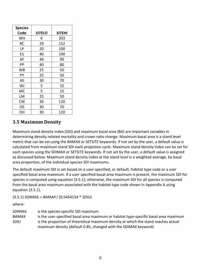
4.1 Height-Diameter Relationships

Height-diameter relationships in FVS are primarily used to estimate tree heights missing in the input data and occasionally to estimate diameter growth on trees smaller than a given threshold diameter. In the CI variant, these relationships are only used to estimate heights missing in the input data, and not to calculate small-tree height growth. Height-diameter relationships are either of a linear form as shown in equation {4.1.2} or a logistic functional form as shown in equation {4.1.1} (Wykoff, et.al 1982). Trees with a DBH greater than 3.0 inches use equation {4.1.1} and trees with a DBH less than or equal to 3.0 inches use equation {4.1.2}. Coefficients for the height-diameter equations are shown are shown in table 4.1.1.

When heights are given in the input data for 3 or more trees of a given species, the value of B1 in equation {4.1.1} for that species is recalculated from the input data and replaces the default value shown in table 4.1.1. In the event that the calculated value is less than zero, the default is used.

{4.1.1} For DBH > 3.0”: HT = 4.5 + exp(B1 + B2 / (DBH + 1.0))

{4.1.2} For DBH < 3.0”: HT = C0 + C1 * DBH

where:

HT is tree height DBH is tree diameter at breast height B1 - B2 are species-specific coefficients shown in table 4.1.1 C0 - C1 are species-specific coefficients shown in table 4.1.1

Table 4.1.1 Coefficients for the height-diameter relationship equations in the CI variant.

Species Code

Default B1 B2 C0 C1

WP 5.19988 -9.26718 1.74189 4.17687 WL 5.16306 -9.25656 5.30838 6.41536 DF 4.94866 -9.75378 3.05990 6.42592 GF 5.02706 -11.21681 2.77647 5.59435 WH 5.02706 -11.21681 2.77647 5.59435 RC 5.16306 -9.25656 5.30838 6.41536 LP 4.80016 -6.51738 0.74322 9.23147 ES 5.09964 -10.79269 2.88424 5.39267 AF 4.91417 -9.36400 2.74231 5.35911 PP 4.99300 -12.430 1.74189 4.17687 WB 4.19200 -5.16510 - -

8

Species Code

Default B1 B2 C0 C1

PY 4.19200 -5.16510 - - AS 4.44210 -6.54050 - - WJ 3.2 -5.0 - - MC 5.1520 -13.5760 0.0994 4.9767 LM 4.19200 -5.16510 - - CW 4.44210 -6.54050 - - OS 4.80016 -6.51738 0.74322 9.23147 OH 4.44210 -6.54050

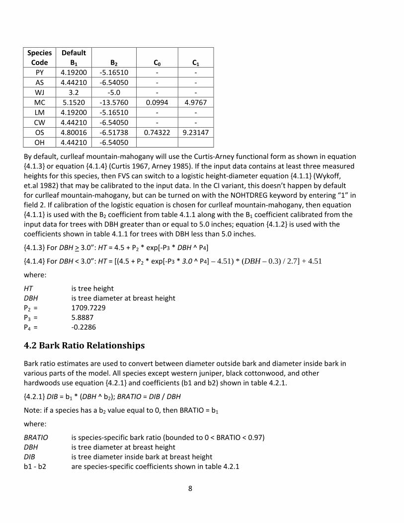
By default, curlleaf mountain-mahogany will use the Curtis-Arney functional form as shown in equation {4.1.3} or equation {4.1.4} (Curtis 1967, Arney 1985). If the input data contains at least three measured heights for this species, then FVS can switch to a logistic height-diameter equation {4.1.1} (Wykoff, et.al 1982) that may be calibrated to the input data. In the CI variant, this doesn’t happen by default for curlleaf mountain-mahogany, but can be turned on with the NOHTDREG keyword by entering “1” in field 2. If calibration of the logistic equation is chosen for curlleaf mountain-mahogany, then equation {4.1.1} is used with the B2 coefficient from table 4.1.1 along with the B1 coefficient calibrated from the input data for trees with DBH greater than or equal to 5.0 inches; equation {4.1.2} is used with the coefficients shown in table 4.1.1 for trees with DBH less than 5.0 inches.

{4.1.3} For DBH > 3.0”: HT = 4.5 + P2 * exp[-P3 * DBH ^ P4]

{4.1.4} For DBH < 3.0”: HT = [(4.5 + P2 * exp[-P3 * 3.0 ^ P4] – 4.51) * (DBH – 0.3) / 2.7] + 4.51

where:

HT is tree height DBH is tree diameter at breast height P2 = 1709.7229 P3 = 5.8887 P4 = -0.2286

4.2 Bark Ratio Relationships

Bark ratio estimates are used to convert between diameter outside bark and diameter inside bark in various parts of the model. All species except western juniper, black cottonwood, and other hardwoods use equation {4.2.1} and coefficients (b1 and b2) shown in table 4.2.1.

{4.2.1} DIB = b1 * (DBH ^ b2); BRATIO = DIB / DBH

Note: if a species has a b2 value equal to 0, then BRATIO = b1

where:

BRATIO is species-specific bark ratio (bounded to 0 < BRATIO < 0.97) DBH is tree diameter at breast height DIB is tree diameter inside bark at breast height b1 - b2 are species-specific coefficients shown in table 4.2.1

9

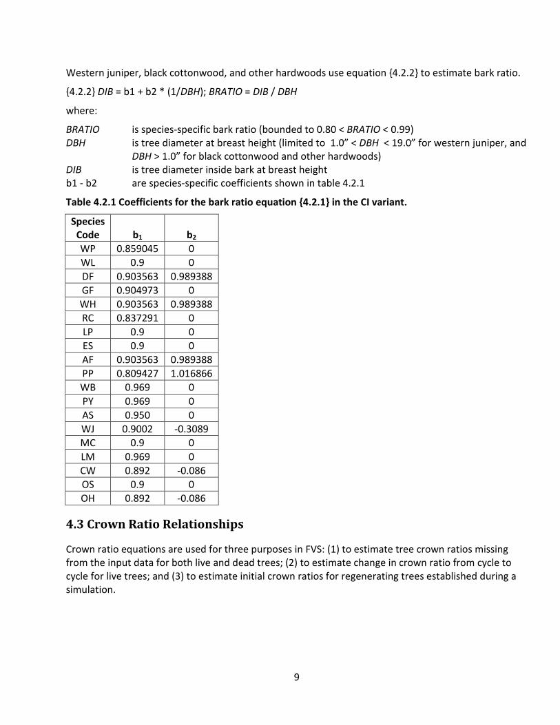
Western juniper, black cottonwood, and other hardwoods use equation {4.2.2} to estimate bark ratio.

{4.2.2} DIB = b1 + b2 * (1/DBH); BRATIO = DIB / DBH

where:

BRATIO is species-specific bark ratio (bounded to 0.80 < BRATIO < 0.99) DBH is tree diameter at breast height (limited to 1.0” < DBH < 19.0” for western juniper, and

DBH > 1.0” for black cottonwood and other hardwoods) DIB is tree diameter inside bark at breast height b1 - b2 are species-specific coefficients shown in table 4.2.1

Table 4.2.1 Coefficients for the bark ratio equation {4.2.1} in the CI variant.

Species Code b1 b2 WP 0.859045 0 WL 0.9 0 DF 0.903563 0.989388 GF 0.904973 0 WH 0.903563 0.989388 RC 0.837291 0 LP 0.9 0 ES 0.9 0 AF 0.903563 0.989388 PP 0.809427 1.016866 WB 0.969 0 PY 0.969 0 AS 0.950 0 WJ 0.9002 -0.3089 MC 0.9 0 LM 0.969 0 CW 0.892 -0.086 OS 0.9 0 OH 0.892 -0.086

4.3 Crown Ratio Relationships

Crown ratio equations are used for three purposes in FVS: (1) to estimate tree crown ratios missing from the input data for both live and dead trees; (2) to estimate change in crown ratio from cycle to cycle for live trees; and (3) to estimate initial crown ratios for regenerating trees established during a simulation.

10

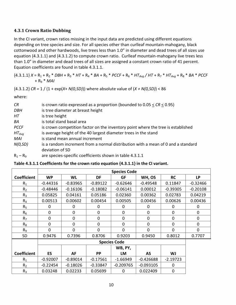
4.3.1 Crown Ratio Dubbing

In the CI variant, crown ratios missing in the input data are predicted using different equations depending on tree species and size. For all species other than curlleaf mountain-mahogany, black cottonwood and other hardwoods, live trees less than 1.0” in diameter and dead trees of all sizes use equation {4.3.1.1} and {4.3.1.2} to compute crown ratio. Curlleaf mountain-mahogany live trees less than 1.0” in diameter and dead trees of all sizes are assigned a constant crown ratio of 41 percent. Equation coefficients are found in table 4.3.1.1.

{4.3.1.1} X = R1 + R2 * DBH + R3 * HT + R4 * BA + R5 * PCCF + R6 * HTAvg / HT + R7 * HTAvg + R8 * BA * PCCF + R9 * MAI

{4.3.1.2} CR = 1 / (1 + exp(X+ N(0,SD))) where absolute value of (X + N(0,SD)) < 86

where:

CR is crown ratio expressed as a proportion (bounded to 0.05 < CR < 0.95) DBH is tree diameter at breast height HT is tree height BA is total stand basal area PCCF is crown competition factor on the inventory point where the tree is established HTAvg is average height of the 40 largest diameter trees in the stand MAI is stand mean annual increment N(0,SD) is a random increment from a normal distribution with a mean of 0 and a standard

deviation of SD R1 – R9 are species-specific coefficients shown in table 4.3.1.1

Table 4.3.1.1 Coefficients for the crown ratio equation {4.3.1.1} in the CI variant.

Coefficient Species Code

WP WL DF GF WH, OS RC LP R1 -0.44316 -0.83965 -0.89122 -0.62646 -0.49548 0.11847 -0.32466 R2 -0.48446 -0.16106 -0.18082 -0.06141 0.00012 -0.39305 -0.20108 R3 0.05825 0.04161 0.05186 0.02360 0.00362 0.02783 0.04219 R4 0.00513 0.00602 0.00454 0.00505 0.00456 0.00626 0.00436 R5 0 0 0 0 0 0 0 R6 0 0 0 0 0 0 0 R7 0 0 0 0 0 0 0 R8 0 0 0 0 0 0 0 R9 0 0 0 0 0 0 0 SD 0.9476 0.7396 0.8706 0.9203 0.9450 0.8012 0.7707

Coefficient

Species Code

ES AF PP WB, PY,

LM AS WJ R1 -0.92007 -0.89014 -0.17561 -1.66949 -0.426688 -2.19723 R2 -0.22454 -0.18026 -0.33847 -0.209765 -0.093105 0 R3 0.03248 0.02233 0.05699 0 0.022409 0

11

R4 0.00620 0.00614 0.00692 0.003359 0.002633 0 R5 0 0 0 0.011032 0 0 R6 0 0 0 0 -0.045532 0 R7 0 0 0 0.017727 0 0 R8 0 0 0 -0.000053 0.000022 0 R9 0 0 0 0.014098 -0.013115 0 SD 0.9721 0.8871 0.8866 0.5 0.9310 0.2

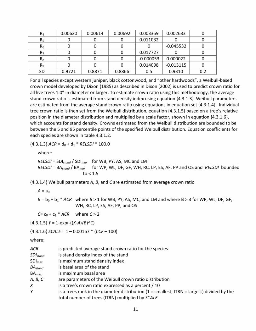
For all species except western juniper, black cottonwood, and “other hardwoods”, a Weibull-based crown model developed by Dixon (1985) as described in Dixon (2002) is used to predict crown ratio for all live trees 1.0” in diameter or larger. To estimate crown ratio using this methodology, the average stand crown ratio is estimated from stand density index using equation {4.3.1.3}. Weibull parameters are estimated from the average stand crown ratio using equations in equation set {4.3.1.4}. Individual tree crown ratio is then set from the Weibull distribution, equation {4.3.1.5} based on a tree’s relative position in the diameter distribution and multiplied by a scale factor, shown in equation {4.3.1.6}, which accounts for stand density. Crowns estimated from the Weibull distribution are bounded to be between the 5 and 95 percentile points of the specified Weibull distribution. Equation coefficients for each species are shown in table 4.3.1.2.

{4.3.1.3} ACR = d0 + d1 * RELSDI * 100.0

where:

RELSDI = SDIstand / SDImax for WB, PY, AS, MC and LM RELSDI = BAstand / BAmax for WP, WL, DF, GF, WH, RC, LP, ES, AF, PP and OS and RELSDI bounded

to < 1.5

{4.3.1.4} Weibull parameters A, B, and C are estimated from average crown ratio

A = a0

B = b0 + b1 * ACR where B > 1 for WB, PY, AS, MC, and LM and where B > 3 for WP, WL, DF, GF, WH, RC, LP, ES, AF, PP, and OS

C= c0 + c1 * ACR where C > 2

{4.3.1.5} Y = 1-exp(-((X-A)/B)^C)

{4.3.1.6} SCALE = 1 – 0.00167 * (CCF – 100)

where:

ACR is predicted average stand crown ratio for the species SDIstand is stand density index of the stand SDImax is maximum stand density index BAstand is basal area of the stand BAmax is maximum basal area A, B, C are parameters of the Weibull crown ratio distribution X is a tree’s crown ratio expressed as a percent / 10 Y is a trees rank in the diameter distribution (1 = smallest; ITRN = largest) divided by the

total number of trees (ITRN) multiplied by SCALE

12

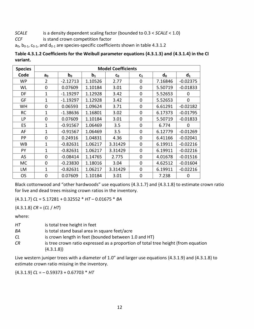
SCALE is a density dependent scaling factor (bounded to 0.3 < SCALE < 1.0) CCF is stand crown competition factor a0, b0-1, c0-1, and d0-1 are species-specific coefficients shown in table 4.3.1.2

Table 4.3.1.2 Coefficients for the Weibull parameter equations {4.3.1.3} and {4.3.1.4} in the CI variant.

Species Code

Model Coefficients a0 b0 b1 c0 c1 d0 d1

WP 2 -2.12713 1.10526 2.77 0 7.16846 -0.02375 WL 0 0.07609 1.10184 3.01 0 5.50719 -0.01833 DF 1 -1.19297 1.12928 3.42 0 5.52653 0 GF 1 -1.19297 1.12928 3.42 0 5.52653 0 WH 0 0.06593 1.09624 3.71 0 6.61291 -0.02182 RC 1 -1.38636 1.16801 3.02 0 6.17373 -0.01795 LP 0 0.07609 1.10184 3.01 0 5.50719 -0.01833 ES 1 -0.91567 1.06469 3.5 0 6.774 0 AF 1 -0.91567 1.06469 3.5 0 6.12779 -0.01269 PP 0 0.24916 1.04831 4.36 0 6.41166 -0.02041 WB 1 -0.82631 1.06217 3.31429 0 6.19911 -0.02216 PY 1 -0.82631 1.06217 3.31429 0 6.19911 -0.02216 AS 0 -0.08414 1.14765 2.775 0 4.01678 -0.01516 MC 0 -0.23830 1.18016 3.04 0 4.62512 -0.01604 LM 1 -0.82631 1.06217 3.31429 0 6.19911 -0.02216 OS 0 0.07609 1.10184 3.01 0 7.238 0

Black cottonwood and “other hardwoods” use equations {4.3.1.7} and {4.3.1.8} to estimate crown ratio for live and dead trees missing crown ratios in the inventory.

{4.3.1.7} CL = 5.17281 + 0.32552 * HT – 0.01675 * BA

{4.3.1.8} CR = (CL / HT)

where:

HT is total tree height in feet BA is total stand basal area in square feet/acre CL is crown length in feet (bounded between 1.0 and HT) CR is tree crown ratio expressed as a proportion of total tree height (from equation

{4.3.1.8})

Live western juniper trees with a diameter of 1.0” and larger use equations {4.3.1.9} and {4.3.1.8} to estimate crown ratio missing in the inventory.

{4.3.1.9} CL = – 0.59373 + 0.67703 * HT

13

4.3.2 Crown Ratio Change

Crown ratio change is estimated after growth, mortality and regeneration are estimated during a projection cycle. Crown ratio change is the difference between the crown ratio at the beginning of the cycle and the predicted crown ratio at the end of the cycle. Crown ratio predicted at the end of the projection cycle is estimated for live tree records using the Weibull distribution, equations {4.3.1.3}-{4.3.1.6}, for all species except black cottonwood, “other hardwoods’, and western juniper. For black cottonwood and “other hardwoods’, crown ratio predicted at the end of the projection cycle is estimated using equations {4.3.1.7} and {4.3.1.8}. For western juniper, crown ratio predicted at the end of the projection cycle is estimated using equations {4.3.1.9} and {4.3.1.8}. Crown change is checked to make sure it doesn’t exceed the change possible if all height growth produces new crown. Crown change is further bounded to 1% per year for the length of the cycle to avoid drastic changes in crown ratio. Equations {4.3.1.1} – {4.3.1.2} are not used when estimating crown ratio change.

4.3.3 Crown Ratio for Newly Established Trees

Crown ratios for newly established trees during regeneration are estimated using equation {4.3.3.1}. A random component is added in equation {4.3.3.1} to ensure that not all newly established trees are assigned exactly the same crown ratio.

{4.3.3.1} CR = 0.89722 – 0.0000461 * PCCF + RAN

where:

CR is crown ratio expressed as a proportion (bounded to 0.2 < CR < 0.9) PCCF is crown competition factor on the inventory point where the tree is established RAN is a small random component

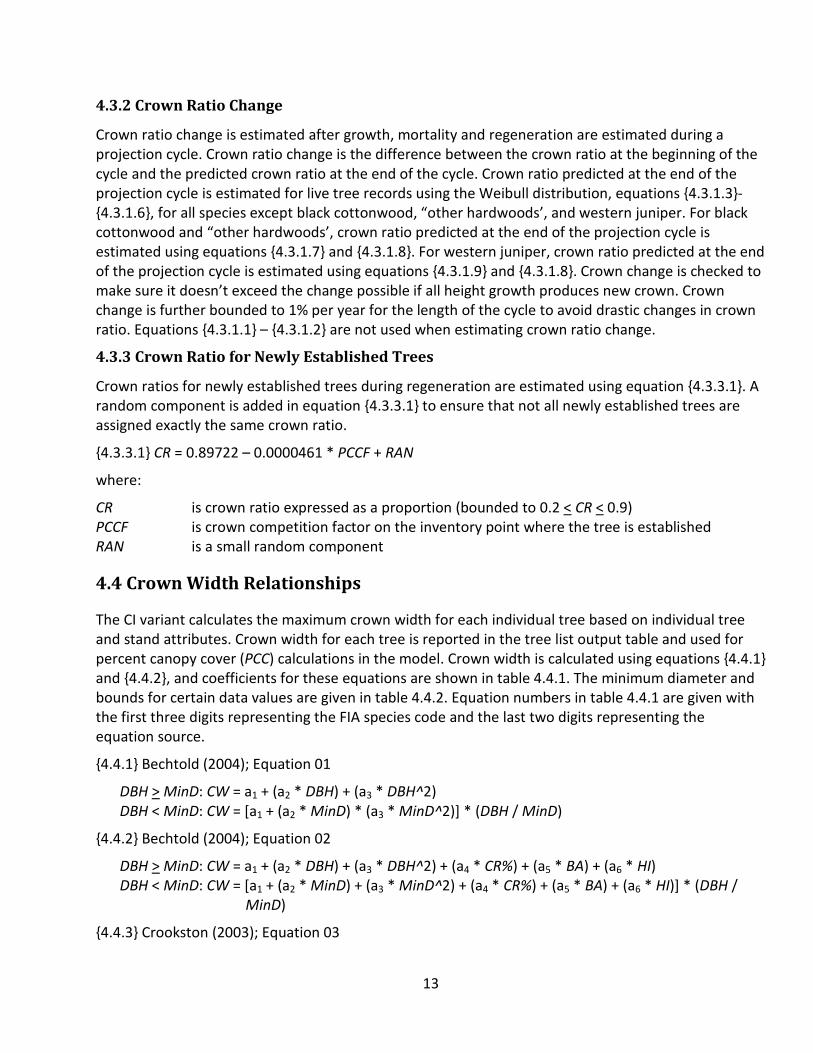
4.4 Crown Width Relationships

The CI variant calculates the maximum crown width for each individual tree based on individual tree and stand attributes. Crown width for each tree is reported in the tree list output table and used for percent canopy cover (PCC) calculations in the model. Crown width is calculated using equations {4.4.1} and {4.4.2}, and coefficients for these equations are shown in table 4.4.1. The minimum diameter and bounds for certain data values are given in table 4.4.2. Equation numbers in table 4.4.1 are given with the first three digits representing the FIA species code and the last two digits representing the equation source.

{4.4.1} Bechtold (2004); Equation 01

DBH > MinD: CW = a1 + (a2 * DBH) + (a3 * DBH^2) DBH < MinD: CW = [a1 + (a2 * MinD) * (a3 * MinD^2)] * (DBH / MinD)

{4.4.2} Bechtold (2004); Equation 02

DBH > MinD: CW = a1 + (a2 * DBH) + (a3 * DBH^2) + (a4 * CR%) + (a5 * BA) + (a6 * HI) DBH < MinD: CW = [a1 + (a2 * MinD) + (a3 * MinD^2) + (a4 * CR%) + (a5 * BA) + (a6 * HI)] * (DBH /

MinD)

{4.4.3} Crookston (2003); Equation 03

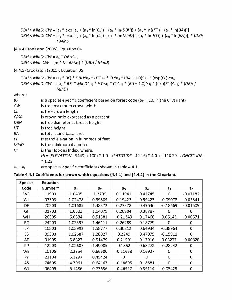
14

DBH > MinD: CW = [a1 * exp [a2 + (a3 * ln(CL)) + (a4 * ln(DBH)) + (a5 * ln(HT)) + (a6 * ln(BA))]] DBH < MinD: CW = [a1 * exp [a2 + (a3 * ln(CL)) + (a4 * ln(MinD) + (a5 * ln(HT)) + (a6 * ln(BA))]] * (DBH

/ MinD)

{4.4.4 Crookston (2005); Equation 04

DBH > MinD: CW = a1 * DBHâ2 DBH < Min: CW = [a1 * MinDâ2] * (DBH / MinD)

{4.4.5} Crookston (2005); Equation 05

DBH > MinD: CW = (a1 * BF) * DBHâ2 * HTâ3 * CLâ4 * (BA + 1.0)â5 * (exp(EL))â6 DBH < MinD: CW = [(a1 * BF) * MinDâ2 * HTâ3 * CLâ4 * (BA + 1.0)â5 * (exp(EL))â6] * (DBH /

MinD) where: BF is a species-specific coefficient based on forest code (BF = 1.0 in the CI variant) CW is tree maximum crown width CL is tree crown length CR% is crown ratio expressed as a percent DBH is tree diameter at breast height HT is tree height BA is total stand basal area EL is stand elevation in hundreds of feet MinD is the minimum diameter HI is the Hopkins Index, where: HI = (ELEVATION - 5449) / 100) * 1.0 + (LATITUDE - 42.16) * 4.0 + (-116.39 - LONGITUDE)

* 1.25 a1 – a6 are species-specific coefficients shown in table 4.4.1

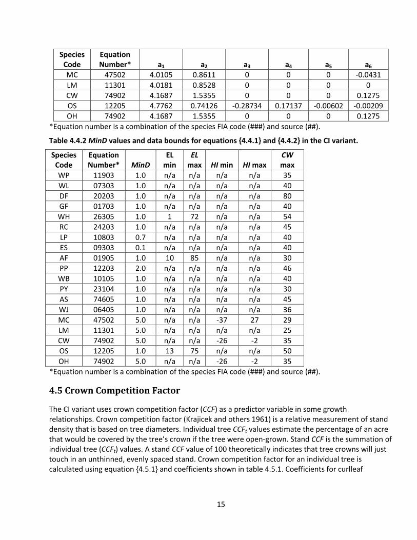
Table 4.4.1 Coefficients for crown width equations {4.4.1} and {4.4.2} in the CI variant.

Species Code

Equation Number* a1 a2 a3 a4 a5 a6

WP 11903 1.0405 1.2799 0.11941 0.42745 0 -0.07182 WL 07303 1.02478 0.99889 0.19422 0.59423 -0.09078 -0.02341 DF 20203 1.01685 1.48372 0.27378 0.49646 -0.18669 -0.01509 GF 01703 1.0303 1.14079 0.20904 0.38787 0 0 WH 26305 6.0384 0.51581 -0.21349 0.17468 0.06143 -0.00571 RC 24203 1.03597 1.46111 0.26289 0.18779 0 0 LP 10803 1.03992 1.58777 0.30812 0.64934 -0.38964 0 ES 09303 1.02687 1.28027 0.2249 0.47075 -0.15911 0 AF 01905 5.8827 0.51479 -0.21501 0.17916 0.03277 -0.00828 PP 12203 1.02687 1.49085 0.1862 0.68272 -0.28242 0 WB 10105 2.2354 0.66680 -0.11658 0.16927 0 0 PY 23104 6.1297 0.45424 0 0 0 0 AS 74605 4.7961 0.64167 -0.18695 0.18581 0 0 WJ 06405 5.1486 0.73636 -0.46927 0.39114 -0.05429 0

15

Species Code

Equation Number* a1 a2 a3 a4 a5 a6

MC 47502 4.0105 0.8611 0 0 0 -0.0431 LM 11301 4.0181 0.8528 0 0 0 0 CW 74902 4.1687 1.5355 0 0 0 0.1275 OS 12205 4.7762 0.74126 -0.28734 0.17137 -0.00602 -0.00209 OH 74902 4.1687 1.5355 0 0 0 0.1275

*Equation number is a combination of the species FIA code (###) and source (##).

Table 4.4.2 MinD values and data bounds for equations {4.4.1} and {4.4.2} in the CI variant.

Species Code

Equation Number* MinD

EL min

EL max HI min HI max

CW max

WP 11903 1.0 n/a n/a n/a n/a 35 WL 07303 1.0 n/a n/a n/a n/a 40 DF 20203 1.0 n/a n/a n/a n/a 80 GF 01703 1.0 n/a n/a n/a n/a 40 WH 26305 1.0 1 72 n/a n/a 54 RC 24203 1.0 n/a n/a n/a n/a 45 LP 10803 0.7 n/a n/a n/a n/a 40 ES 09303 0.1 n/a n/a n/a n/a 40 AF 01905 1.0 10 85 n/a n/a 30 PP 12203 2.0 n/a n/a n/a n/a 46 WB 10105 1.0 n/a n/a n/a n/a 40 PY 23104 1.0 n/a n/a n/a n/a 30 AS 74605 1.0 n/a n/a n/a n/a 45 WJ 06405 1.0 n/a n/a n/a n/a 36 MC 47502 5.0 n/a n/a -37 27 29 LM 11301 5.0 n/a n/a n/a n/a 25 CW 74902 5.0 n/a n/a -26 -2 35 OS 12205 1.0 13 75 n/a n/a 50 OH 74902 5.0 n/a n/a -26 -2 35

*Equation number is a combination of the species FIA code (###) and source (##).

4.5 Crown Competition Factor

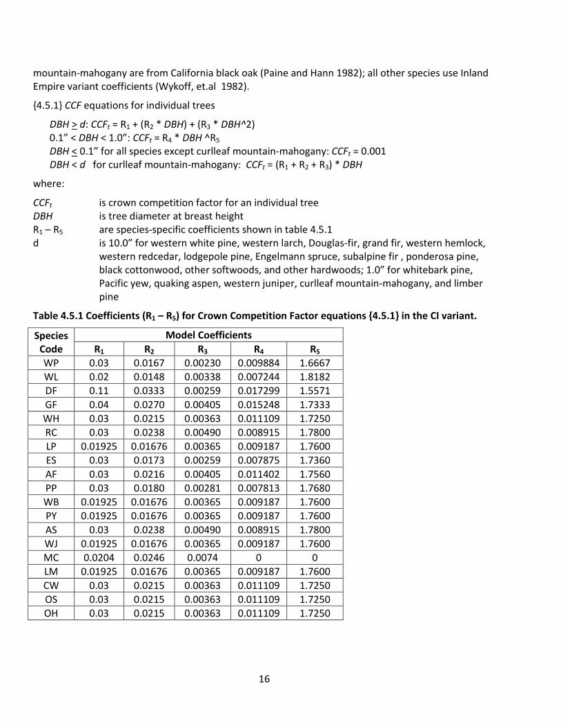
The CI variant uses crown competition factor (CCF) as a predictor variable in some growth relationships. Crown competition factor (Krajicek and others 1961) is a relative measurement of stand density that is based on tree diameters. Individual tree CCFt values estimate the percentage of an acre that would be covered by the tree’s crown if the tree were open-grown. Stand CCF is the summation of individual tree (CCFt) values. A stand CCF value of 100 theoretically indicates that tree crowns will just touch in an unthinned, evenly spaced stand. Crown competition factor for an individual tree is calculated using equation {4.5.1} and coefficients shown in table 4.5.1. Coefficients for curlleaf

16

mountain-mahogany are from California black oak (Paine and Hann 1982); all other species use Inland Empire variant coefficients (Wykoff, et.al 1982).

{4.5.1} CCF equations for individual trees

DBH > d: CCFt = R1 + (R2 * DBH) + (R3 * DBH^2) 0.1” < DBH < 1.0”: CCFt = R4 * DBH ^R5 DBH < 0.1” for all species except curlleaf mountain-mahogany: CCFt = 0.001 DBH < d for curlleaf mountain-mahogany: CCFt = (R1 + R2 + R3) * DBH

where:

CCFt is crown competition factor for an individual tree DBH is tree diameter at breast height R1 – R5 are species-specific coefficients shown in table 4.5.1 d is 10.0” for western white pine, western larch, Douglas-fir, grand fir, western hemlock,

western redcedar, lodgepole pine, Engelmann spruce, subalpine fir , ponderosa pine, black cottonwood, other softwoods, and other hardwoods; 1.0” for whitebark pine, Pacific yew, quaking aspen, western juniper, curlleaf mountain-mahogany, and limber pine

Table 4.5.1 Coefficients (R1 – R5) for Crown Competition Factor equations {4.5.1} in the CI variant.

Species Code

Model Coefficients R1 R2 R3 R4 R5

WP 0.03 0.0167 0.00230 0.009884 1.6667 WL 0.02 0.0148 0.00338 0.007244 1.8182 DF 0.11 0.0333 0.00259 0.017299 1.5571 GF 0.04 0.0270 0.00405 0.015248 1.7333 WH 0.03 0.0215 0.00363 0.011109 1.7250 RC 0.03 0.0238 0.00490 0.008915 1.7800 LP 0.01925 0.01676 0.00365 0.009187 1.7600 ES 0.03 0.0173 0.00259 0.007875 1.7360 AF 0.03 0.0216 0.00405 0.011402 1.7560 PP 0.03 0.0180 0.00281 0.007813 1.7680 WB 0.01925 0.01676 0.00365 0.009187 1.7600 PY 0.01925 0.01676 0.00365 0.009187 1.7600 AS 0.03 0.0238 0.00490 0.008915 1.7800 WJ 0.01925 0.01676 0.00365 0.009187 1.7600 MC 0.0204 0.0246 0.0074 0 0 LM 0.01925 0.01676 0.00365 0.009187 1.7600 CW 0.03 0.0215 0.00363 0.011109 1.7250 OS 0.03 0.0215 0.00363 0.011109 1.7250 OH 0.03 0.0215 0.00363 0.011109 1.7250

17

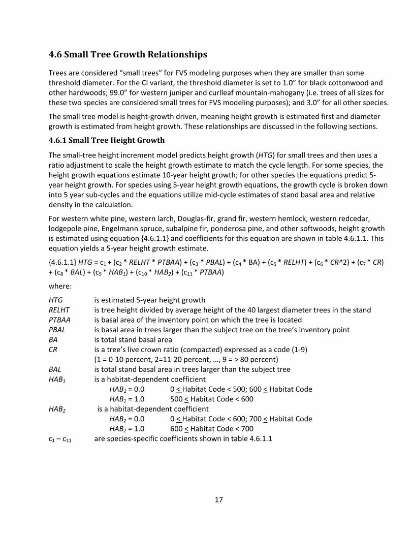
4.6 Small Tree Growth Relationships

Trees are considered “small trees” for FVS modeling purposes when they are smaller than some threshold diameter. For the CI variant, the threshold diameter is set to 1.0” for black cottonwood and other hardwoods; 99.0” for western juniper and curlleaf mountain-mahogany (i.e. trees of all sizes for these two species are considered small trees for FVS modeling purposes); and 3.0” for all other species.

The small tree model is height-growth driven, meaning height growth is estimated first and diameter growth is estimated from height growth. These relationships are discussed in the following sections.

4.6.1 Small Tree Height Growth

The small-tree height increment model predicts height growth (HTG) for small trees and then uses a ratio adjustment to scale the height growth estimate to match the cycle length. For some species, the height growth equations estimate 10-year height growth; for other species the equations predict 5-year height growth. For species using 5-year height growth equations, the growth cycle is broken down into 5 year sub-cycles and the equations utilize mid-cycle estimates of stand basal area and relative density in the calculation.

For western white pine, western larch, Douglas-fir, grand fir, western hemlock, western redcedar, lodgepole pine, Engelmann spruce, subalpine fir, ponderosa pine, and other softwoods, height growth is estimated using equation {4.6.1.1} and coefficients for this equation are shown in table 4.6.1.1. This equation yields a 5-year height growth estimate.

{4.6.1.1} HTG = c1 + (c2 * RELHT * PTBAA) + (c3 * PBAL) + (c4 * BA) + (c5 * RELHT) + (c6 * CR^2) + (c7 * CR) + (c8 * BAL) + (c9 * HAB1) + (c10 * HAB2) + (c11 * PTBAA)

where:

HTG is estimated 5-year height growth RELHT is tree height divided by average height of the 40 largest diameter trees in the stand PTBAA is basal area of the inventory point on which the tree is located PBAL is basal area in trees larger than the subject tree on the tree’s inventory point BA is total stand basal area CR is a tree’s live crown ratio (compacted) expressed as a code (1-9) (1 = 0-10 percent, 2=11-20 percent, …, 9 = > 80 percent) BAL is total stand basal area in trees larger than the subject tree HAB1 is a habitat-dependent coefficient

HAB1 = 0.0 0 < Habitat Code < 500; 600 < Habitat Code HAB1 = 1.0 500 < Habitat Code < 600

HAB2 is a habitat-dependent coefficient HAB2 = 0.0 0 < Habitat Code < 600; 700 < Habitat Code HAB2 = 1.0 600 < Habitat Code < 700

c1 – c11 are species-specific coefficients shown in table 4.6.1.1

18

Table 4.6.1.1 Coefficients (c1 – c11) for equation {4.6.1.1} in the CI variant.

Species Code

Coefficients c1 c2 c3 c4 c5 c6

WP 1.59898 0 -0.00203 0 1.36048 0.01998 WL 1.59898 0 -0.00203 0 1.36048 0.01998 DF 1.59898 0 -0.00203 0 1.36048 0.01998 GF 1.22213 0.00788 -0.00187 -0.00158 0.62556 0.02788 WH 1.22213 0.00788 -0.00187 -0.00158 0.62556 0.02788 RC 1.59898 0 -0.00203 0 1.36048 0.01998 LP 2.13400 -0.01040 0 -0.05702 2.55943 0.05926 ES 1.76880 0 -0.00163 0 1.56488 0.03346 AF 1.25335 0 -0.04330 0 1.91954 0.03055 PP 2.76456 0 0 -0.00964 0 0.02530 OS 2.13400 -0.01040 0 -0.05702 2.55943 0.05926

Species Code

Coefficients c7 c8 c9 c10 c11

WP 0 -0.00424 0 0 0 WL 0 -0.00424 0 0 0 DF 0 -0.00424 0 0 0 GF -0.05668 0 -0.14824 0 0 WH -0.05668 0 -0.14824 0 0 RC 0 -0.00424 0 0 0 LP -0.42992 0.04685 1.34457 0.94168 0 ES -0.24019 -0.00258 0 -0.17039 0 AF -0.18446 0 0 -0.35149 0.04162 PP 0 0 0 0 0 OS -0.42992 0.04685 1.34457 0.94168 0

For western juniper, curlleaf mountain-mahogany, black cottonwood, and other hardwoods, the small-tree height increment model predicts 10-year height growth (HTG) for small trees based on site index, and is then modified to account for density effects and tree vigor.

Potential height growth for these four species is estimated using equation {4.6.1.2}.

{4.6.1.2} POTHTG = ((SI / 5.0) * (SI * 1.5 - H) / (SI * 1.5)) * 0.83

where:

POTHTG is potential height growth SI is species site index on a base-age basis H is tree height

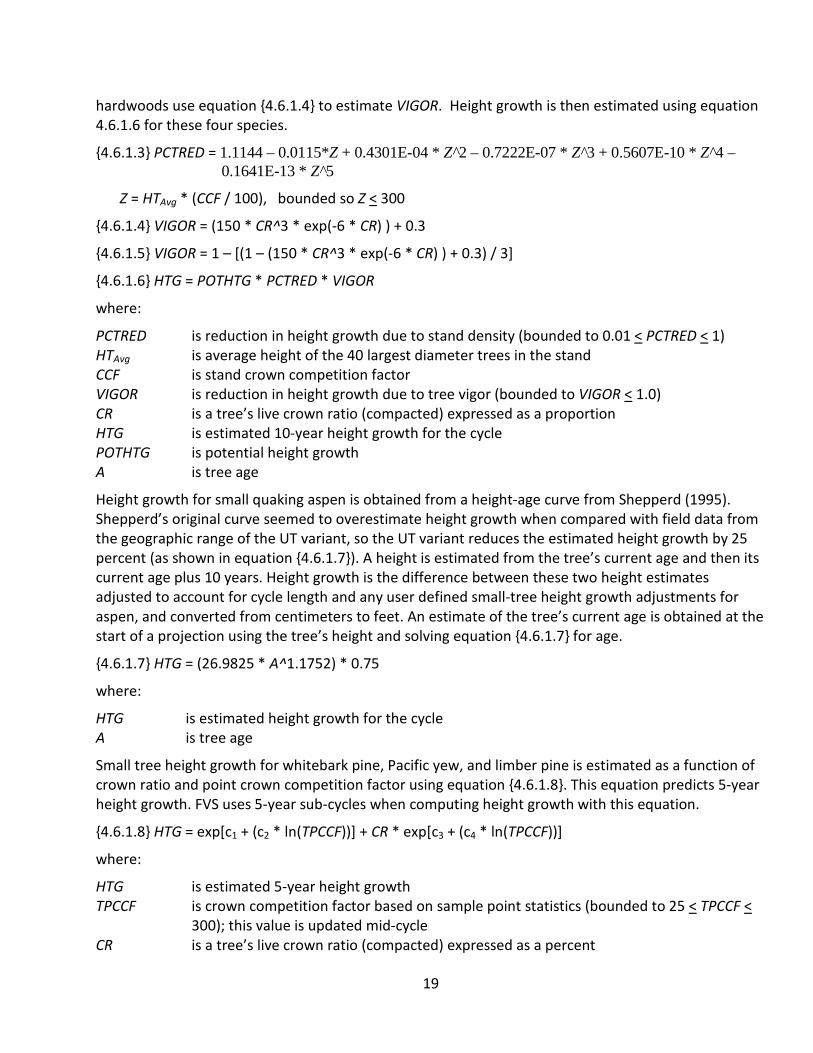
Potential height growth is then adjusted based on stand density (PCTRED) as computed with equation {4.6.1.3}, and crown ratio (VIGOR) as shown in equation {4.6.1.4} or {4.6.1.5}. Western juniper uses equation {4.6.1.5} to estimate VIGOR; curlleaf mountain-mahogany, black cottonwood, and other

19

hardwoods use equation {4.6.1.4} to estimate VIGOR. Height growth is then estimated using equation 4.6.1.6 for these four species.

{4.6.1.3} PCTRED = 1.1144 – 0.0115*Z + 0.4301E-04 * Z^2 – 0.7222E-07 * Z^3 + 0.5607E-10 * Z^4 – 0.1641E-13 * Z^5

Z = HTAvg * (CCF / 100), bounded so Z < 300

{4.6.1.4} VIGOR = (150 * CR^3 * exp(-6 * CR) ) + 0.3

{4.6.1.5} VIGOR = 1 – [(1 – (150 * CR^3 * exp(-6 * CR) ) + 0.3) / 3]

{4.6.1.6} HTG = POTHTG * PCTRED * VIGOR

where:

PCTRED is reduction in height growth due to stand density (bounded to 0.01 < PCTRED < 1) HTAvg is average height of the 40 largest diameter trees in the stand CCF is stand crown competition factor VIGOR is reduction in height growth due to tree vigor (bounded to VIGOR < 1.0) CR is a tree’s live crown ratio (compacted) expressed as a proportion HTG is estimated 10-year height growth for the cycle POTHTG is potential height growth A is tree age

Height growth for small quaking aspen is obtained from a height-age curve from Shepperd (1995). Shepperd’s original curve seemed to overestimate height growth when compared with field data from the geographic range of the UT variant, so the UT variant reduces the estimated height growth by 25 percent (as shown in equation {4.6.1.7}). A height is estimated from the tree’s current age and then its current age plus 10 years. Height growth is the difference between these two height estimates adjusted to account for cycle length and any user defined small-tree height growth adjustments for aspen, and converted from centimeters to feet. An estimate of the tree’s current age is obtained at the start of a projection using the tree’s height and solving equation {4.6.1.7} for age.

{4.6.1.7} HTG = (26.9825 * A^1.1752) * 0.75

where:

HTG is estimated height growth for the cycle A is tree age

Small tree height growth for whitebark pine, Pacific yew, and limber pine is estimated as a function of crown ratio and point crown competition factor using equation {4.6.1.8}. This equation predicts 5-year height growth. FVS uses 5-year sub-cycles when computing height growth with this equation.

{4.6.1.8} HTG = exp[c1 + (c2 * ln(TPCCF))] + CR * exp[c3 + (c4 * ln(TPCCF))]

where:

HTG is estimated 5-year height growth TPCCF is crown competition factor based on sample point statistics (bounded to 25 < TPCCF <

300); this value is updated mid-cycle CR is a tree’s live crown ratio (compacted) expressed as a percent

20

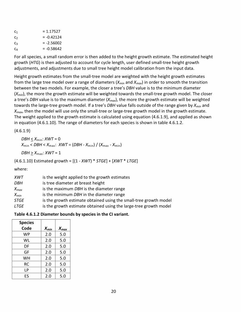
c1 = 1.17527 c2 = -0.42124 c3 = -2.56002 c4 = -0.58642

For all species, a small random error is then added to the height growth estimate. The estimated height growth (HTG) is then adjusted to account for cycle length, user defined small-tree height growth adjustments, and adjustments due to small tree height model calibration from the input data.

Height growth estimates from the small-tree model are weighted with the height growth estimates from the large tree model over a range of diameters (Xmin and Xmax) in order to smooth the transition between the two models. For example, the closer a tree’s DBH value is to the minimum diameter (Xmin), the more the growth estimate will be weighted towards the small-tree growth model. The closer a tree’s DBH value is to the maximum diameter (Xmax), the more the growth estimate will be weighted towards the large-tree growth model. If a tree’s DBH value falls outside of the range given by Xmin and Xmax, then the model will use only the small-tree or large-tree growth model in the growth estimate. The weight applied to the growth estimate is calculated using equation {4.6.1.9}, and applied as shown in equation {4.6.1.10}. The range of diameters for each species is shown in table 4.6.1.2.

{4.6.1.9}

DBH < Xmin: XWT = 0 Xmin < DBH < Xmax: XWT = (DBH - Xmin) / (Xmax - Xmin)

DBH > Xmax: XWT = 1

{4.6.1.10} Estimated growth = [(1 - XWT) * STGE] + [XWT * LTGE]

where:

XWT is the weight applied to the growth estimates DBH is tree diameter at breast height Xmax is the maximum DBH is the diameter range Xmin is the minimum DBH in the diameter range STGE is the growth estimate obtained using the small-tree growth model LTGE is the growth estimate obtained using the large-tree growth model

Table 4.6.1.2 Diameter bounds by species in the CI variant.

Species Code Xmin Xmax WP 2.0 5.0 WL 2.0 5.0 DF 2.0 5.0 GF 2.0 5.0 WH 2.0 5.0 RC 2.0 5.0 LP 2.0 5.0 ES 2.0 5.0

21

Species Code Xmin Xmax

AF 2.0 5.0 PP 2.0 5.0 WB 1.5 3.0 PY 1.5 3.0 AS 2.0 4.0 WJ 90. 99. MC 90. 99. LM 1.5 3.0 CW 0.5 2.0 OS 2.0 5.0 OH 0.5 2.0

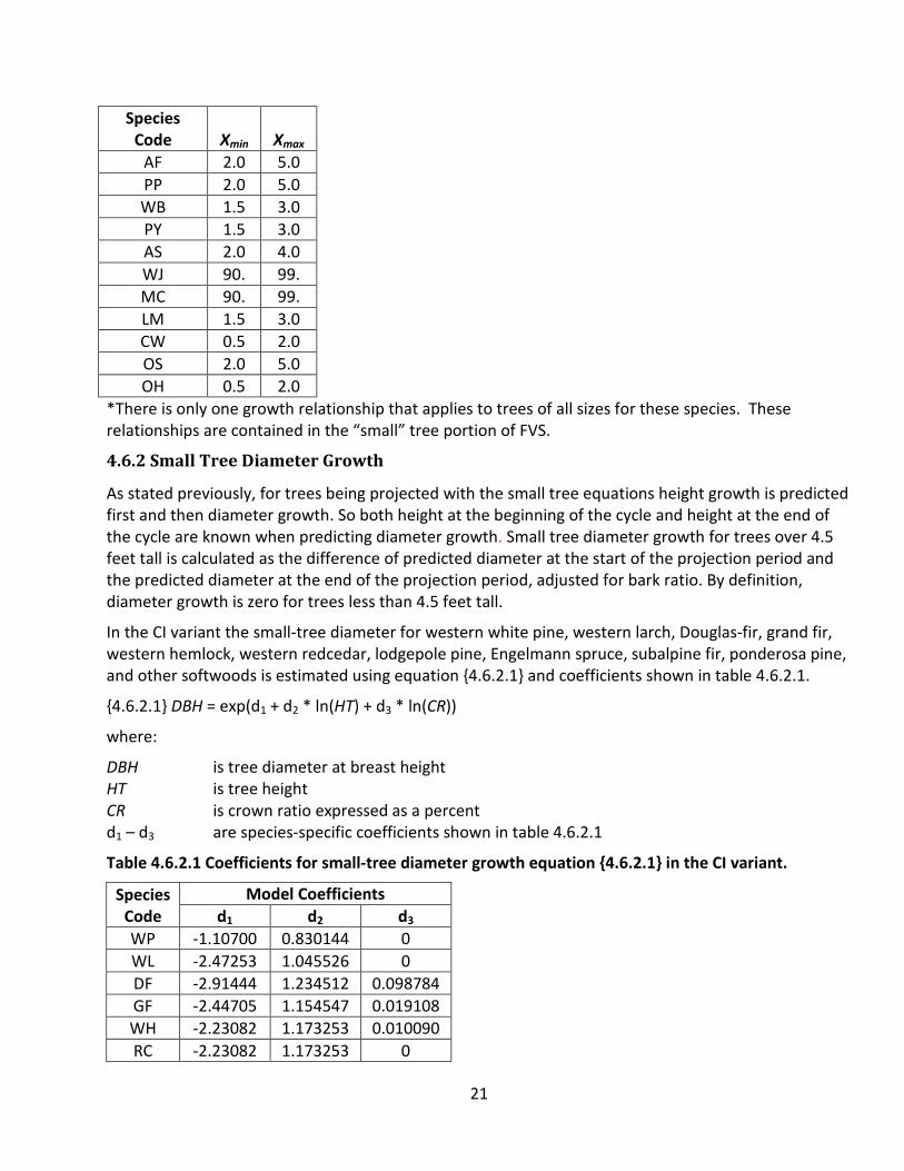
*There is only one growth relationship that applies to trees of all sizes for these species. These relationships are contained in the “small” tree portion of FVS.

4.6.2 Small Tree Diameter Growth

As stated previously, for trees being projected with the small tree equations height growth is predicted first and then diameter growth. So both height at the beginning of the cycle and height at the end of the cycle are known when predicting diameter growth. Small tree diameter growth for trees over 4.5 feet tall is calculated as the difference of predicted diameter at the start of the projection period and the predicted diameter at the end of the projection period, adjusted for bark ratio. By definition, diameter growth is zero for trees less than 4.5 feet tall.

In the CI variant the small-tree diameter for western white pine, western larch, Douglas-fir, grand fir, western hemlock, western redcedar, lodgepole pine, Engelmann spruce, subalpine fir, ponderosa pine, and other softwoods is estimated using equation {4.6.2.1} and coefficients shown in table 4.6.2.1.

{4.6.2.1} DBH = exp(d1 + d2 * ln(HT) + d3 * ln(CR))

where:

DBH is tree diameter at breast height HT is tree height CR is crown ratio expressed as a percent d1 – d3 are species-specific coefficients shown in table 4.6.2.1

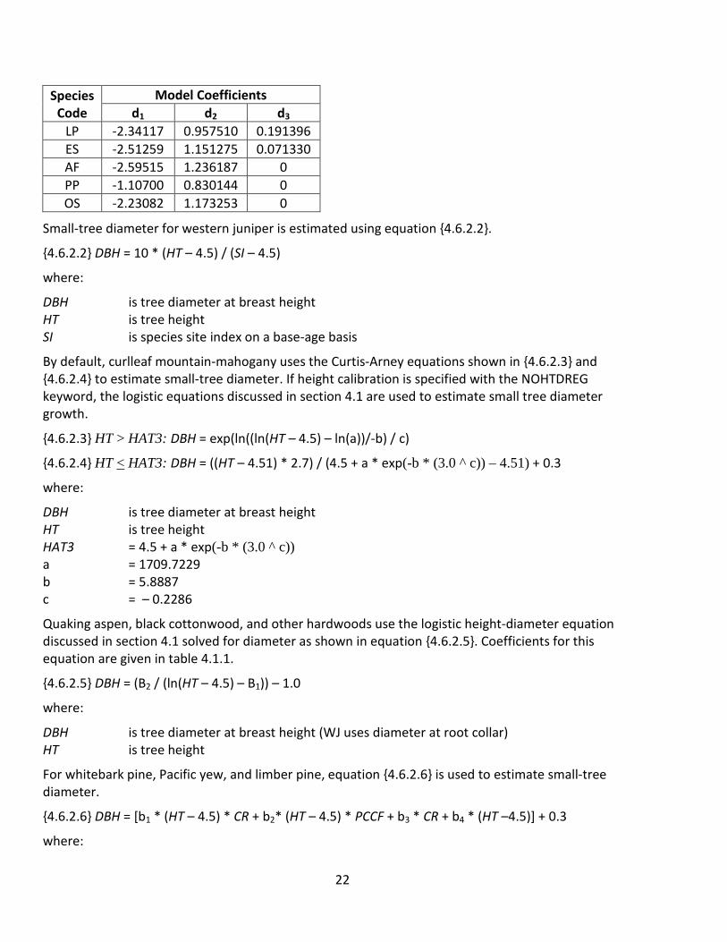
Table 4.6.2.1 Coefficients for small-tree diameter growth equation {4.6.2.1} in the CI variant.

Species Code

Model Coefficients d1 d2 d3

WP -1.10700 0.830144 0 WL -2.47253 1.045526 0 DF -2.91444 1.234512 0.098784 GF -2.44705 1.154547 0.019108 WH -2.23082 1.173253 0.010090 RC -2.23082 1.173253 0

22

Species Code

Model Coefficients d1 d2 d3

LP -2.34117 0.957510 0.191396 ES -2.51259 1.151275 0.071330 AF -2.59515 1.236187 0 PP -1.10700 0.830144 0 OS -2.23082 1.173253 0

Small-tree diameter for western juniper is estimated using equation {4.6.2.2}.

{4.6.2.2} DBH = 10 * (HT – 4.5) / (SI – 4.5)

where:

DBH is tree diameter at breast height HT is tree height SI is species site index on a base-age basis

By default, curlleaf mountain-mahogany uses the Curtis-Arney equations shown in {4.6.2.3} and {4.6.2.4} to estimate small-tree diameter. If height calibration is specified with the NOHTDREG keyword, the logistic equations discussed in section 4.1 are used to estimate small tree diameter growth.

{4.6.2.3} HT > HAT3: DBH = exp(ln((ln(HT – 4.5) – ln(a))/-b) / c)

{4.6.2.4} HT < HAT3: DBH = ((HT – 4.51) * 2.7) / (4.5 + a * exp(-b * (3.0 ^ c)) – 4.51) + 0.3

where:

DBH is tree diameter at breast height HT is tree height HAT3 = 4.5 + a * exp(-b * (3.0 ^ c)) a = 1709.7229 b = 5.8887 c = – 0.2286

Quaking aspen, black cottonwood, and other hardwoods use the logistic height-diameter equation discussed in section 4.1 solved for diameter as shown in equation {4.6.2.5}. Coefficients for this equation are given in table 4.1.1.

{4.6.2.5} DBH = (B2 / (ln(HT – 4.5) – B1)) – 1.0

where:

DBH is tree diameter at breast height (WJ uses diameter at root collar) HT is tree height

For whitebark pine, Pacific yew, and limber pine, equation {4.6.2.6} is used to estimate small-tree diameter.

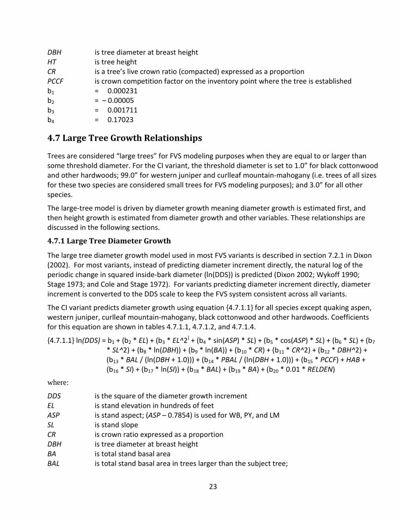
{4.6.2.6} DBH = [b1 * (HT – 4.5) * CR + b2* (HT – 4.5) * PCCF + b3 * CR + b4 * (HT –4.5)] + 0.3

where:

23

DBH is tree diameter at breast height HT is tree height CR is a tree’s live crown ratio (compacted) expressed as a proportion PCCF is crown competition factor on the inventory point where the tree is established b1 = 0.000231 b2 = – 0.00005 b3 = 0.001711 b4 = 0.17023

4.7 Large Tree Growth Relationships

Trees are considered “large trees” for FVS modeling purposes when they are equal to or larger than some threshold diameter. For the CI variant, the threshold diameter is set to 1.0” for black cottonwood and other hardwoods; 99.0” for western juniper and curlleaf mountain-mahogany (i.e. trees of all sizes for these two species are considered small trees for FVS modeling purposes); and 3.0” for all other species.

The large-tree model is driven by diameter growth meaning diameter growth is estimated first, and then height growth is estimated from diameter growth and other variables. These relationships are discussed in the following sections.

4.7.1 Large Tree Diameter Growth

The large tree diameter growth model used in most FVS variants is described in section 7.2.1 in Dixon (2002). For most variants, instead of predicting diameter increment directly, the natural log of the periodic change in squared inside-bark diameter (ln(DDS)) is predicted (Dixon 2002; Wykoff 1990; Stage 1973; and Cole and Stage 1972). For variants predicting diameter increment directly, diameter increment is converted to the DDS scale to keep the FVS system consistent across all variants.

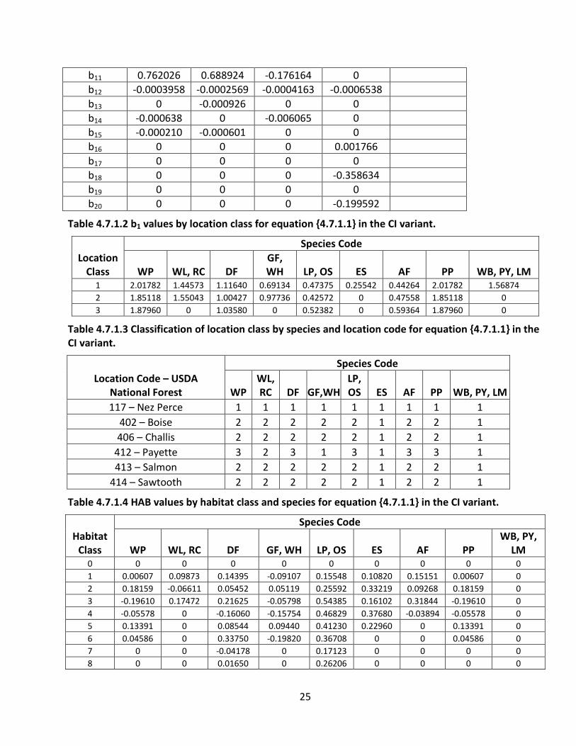
The CI variant predicts diameter growth using equation {4.7.1.1} for all species except quaking aspen, western juniper, curlleaf mountain-mahogany, black cottonwood and other hardwoods. Coefficients for this equation are shown in tables 4.7.1.1, 4.7.1.2, and 4.7.1.4.

{4.7.1.1} ln(DDS) = b1 + (b2 * EL) + (b3 * EL^2) + (b4 * sin(ASP) * SL) + (b5 * cos(ASP) * SL) + (b6 * SL) + (b7 * SL^2) + (b8 * ln(DBH)) + (b9 * ln(BA)) + (b10 * CR) + (b11 * CR^2) + (b12 * DBH^2) + (b13 * BAL / (ln(DBH + 1.0))) + (b14 * PBAL / (ln(DBH + 1.0))) + (b15 * PCCF) + HAB + (b16 * SI) + (b17 * ln(SI)) + (b18 * BAL) + (b19 * BA) + (b20 * 0.01 * RELDEN)

where:

DDS is the square of the diameter growth increment EL is stand elevation in hundreds of feet ASP is stand aspect; (ASP – 0.7854) is used for WB, PY, and LM SL is stand slope CR is crown ratio expressed as a proportion DBH is tree diameter at breast height BA is total stand basal area BAL is total stand basal area in trees larger than the subject tree;

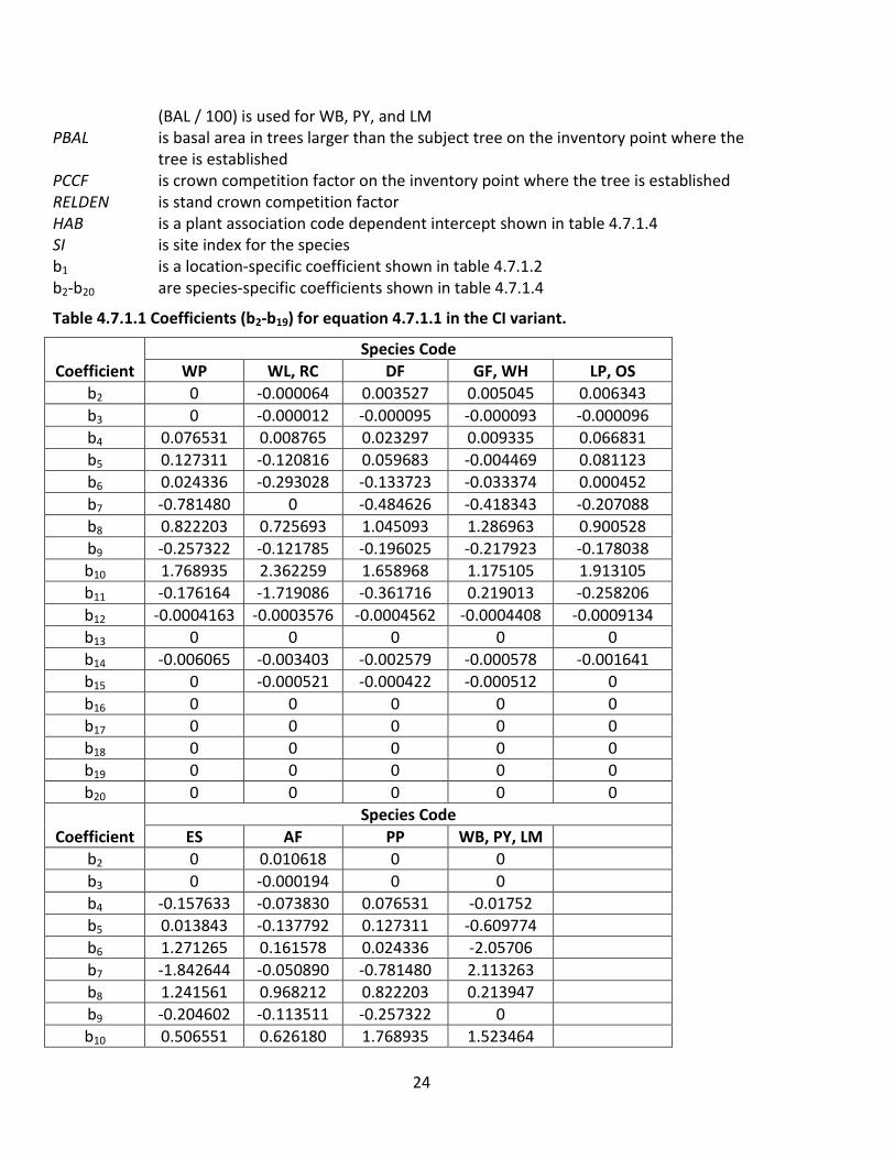
24

(BAL / 100) is used for WB, PY, and LM PBAL is basal area in trees larger than the subject tree on the inventory point where the tree is established PCCF is crown competition factor on the inventory point where the tree is established RELDEN is stand crown competition factor HAB is a plant association code dependent intercept shown in table 4.7.1.4 SI is site index for the species b1 is a location-specific coefficient shown in table 4.7.1.2 b2-b20 are species-specific coefficients shown in table 4.7.1.4

Table 4.7.1.1 Coefficients (b2-b19) for equation 4.7.1.1 in the CI variant.


WP WL, RC DF GF, WH LP, OS b2 0 -0.000064 0.003527 0.005045 0.006343 b3 0 -0.000012 -0.000095 -0.000093 -0.000096 b4 0.076531 0.008765 0.023297 0.009335 0.066831 b5 0.127311 -0.120816 0.059683 -0.004469 0.081123 b6 0.024336 -0.293028 -0.133723 -0.033374 0.000452 b7 -0.781480 0 -0.484626 -0.418343 -0.207088 b8 0.822203 0.725693 1.045093 1.286963 0.900528 b9 -0.257322 -0.121785 -0.196025 -0.217923 -0.178038 b10 1.768935 2.362259 1.658968 1.175105 1.913105 b11 -0.176164 -1.719086 -0.361716 0.219013 -0.258206 b12 -0.0004163 -0.0003576 -0.0004562 -0.0004408 -0.0009134 b13 0 0 0 0 0 b14 -0.006065 -0.003403 -0.002579 -0.000578 -0.001641 b15 0 -0.000521 -0.000422 -0.000512 0 b16 0 0 0 0 0 b17 0 0 0 0 0 b18 0 0 0 0 0 b19 0 0 0 0 0 b20 0 0 0 0 0


ES AF PP WB, PY, LM b2 0 0.010618 0 0 b3 0 -0.000194 0 0 b4 -0.157633 -0.073830 0.076531 -0.01752 b5 0.013843 -0.137792 0.127311 -0.609774 b6 1.271265 0.161578 0.024336 -2.05706 b7 -1.842644 -0.050890 -0.781480 2.113263 b8 1.241561 0.968212 0.822203 0.213947 b9 -0.204602 -0.113511 -0.257322 0 b10 0.506551 0.626180 1.768935 1.523464

25

b11 0.762026 0.688924 -0.176164 0 b12 -0.0003958 -0.0002569 -0.0004163 -0.0006538 b13 0 -0.000926 0 0 b14 -0.000638 0 -0.006065 0 b15 -0.000210 -0.000601 0 0 b16 0 0 0 0.001766 b17 0 0 0 0 b18 0 0 0 -0.358634 b19 0 0 0 0 b20 0 0 0 -0.199592

Table 4.7.1.2 b1 values by location class for equation {4.7.1.1} in the CI variant.

Location Class

Species Code

WP WL, RC DF GF, WH LP, OS ES AF PP WB, PY, LM

1 2.01782 1.44573 1.11640 0.69134 0.47375 0.25542 0.44264 2.01782 1.56874 2 1.85118 1.55043 1.00427 0.97736 0.42572 0 0.47558 1.85118 0 3 1.87960 0 1.03580 0 0.52382 0 0.59364 1.87960 0

Table 4.7.1.3 Classification of location class by species and location code for equation {4.7.1.1} in the CI variant.

Location Code – USDA National Forest

Species Code

WP WL, RC DF GF,WH

LP, OS ES AF PP WB, PY, LM

117 – Nez Perce 1 1 1 1 1 1 1 1 1 402 – Boise 2 2 2 2 2 1 2 2 1 406 – Challis 2 2 2 2 2 1 2 2 1

412 – Payette 3 2 3 1 3 1 3 3 1 413 – Salmon 2 2 2 2 2 1 2 2 1

414 – Sawtooth 2 2 2 2 2 1 2 2 1

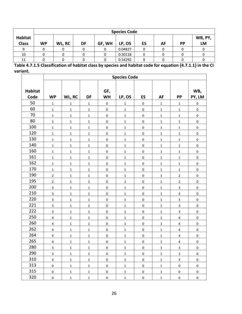
Table 4.7.1.4 HAB values by habitat class and species for equation {4.7.1.1} in the CI variant.

Habitat Class

Species Code

WP WL, RC DF GF, WH LP, OS ES AF PP WB, PY,

LM 0 0 0 0 0 0 0 0 0 0 1 0.00607 0.09873 0.14395 -0.09107 0.15548 0.10820 0.15151 0.00607 0 2 0.18159 -0.06611 0.05452 0.05119 0.25592 0.33219 0.09268 0.18159 0 3 -0.19610 0.17472 0.21625 -0.05798 0.54385 0.16102 0.31844 -0.19610 0 4 -0.05578 0 -0.16060 -0.15754 0.46829 0.37680 -0.03894 -0.05578 0 5 0.13391 0 0.08544 0.09440 0.41230 0.22960 0 0.13391 0 6 0.04586 0 0.33750 -0.19820 0.36708 0 0 0.04586 0 7 0 0 -0.04178 0 0.17123 0 0 0 0 8 0 0 0.01650 0 0.26206 0 0 0 0

26

Habitat Class

Species Code

WP WL, RC DF GF, WH LP, OS ES AF PP WB, PY,

LM 9 0 0 0 0 0.04827 0 0 0 0

10 0 0 0 0 0.30118 0 0 0 0 11 0 0 0 0 0.54292 0 0 0 0

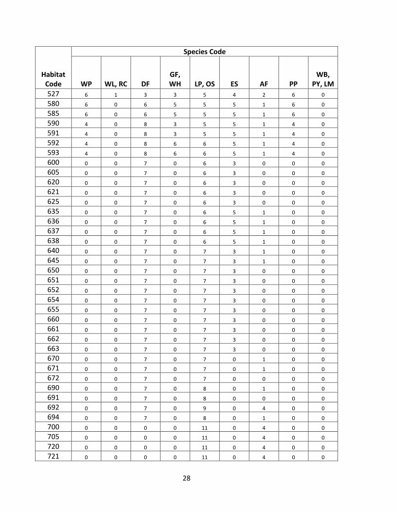
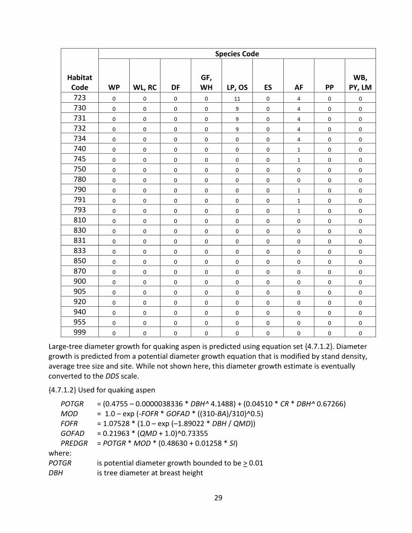
Table 4.7.1.5 Classification of habitat class by species and habitat code for equation {4.7.1.1} in the CI variant.

Habitat Code

Species Code

WP WL, RC DF GF, WH LP, OS ES AF PP

WB, PY, LM

50 1 1 1 0 1 0 1 1 0

60 1 1 1 0 1 0 1 1 0

70 1 1 1 0 1 0 1 1 0

80 1 1 1 0 1 0 1 1 0

100 1 1 1 0 1 0 1 1 0

120 1 1 1 0 1 0 1 1 0

130 1 1 1 0 1 0 1 1 0

140 1 1 1 0 1 0 1 1 0

160 1 1 1 0 1 0 1 1 0

161 1 1 1 0 1 0 1 1 0

162 1 1 1 0 1 0 1 1 0

170 1 1 1 0 1 0 1 1 0

190 2 1 1 0 1 0 1 2 0

195 2 1 1 0 1 0 1 2 0

200 3 1 1 0 1 0 1 3 0

210 3 1 1 0 1 0 1 3 0

220 3 1 1 0 1 0 1 3 0

221 3 1 1 0 1 0 1 3 0

222 3 1 1 0 1 0 1 3 0

250 4 1 1 0 1 0 1 4 0

260 4 1 1 0 1 0 1 4 0

262 4 1 1 0 1 0 1 4 0

264 4 1 1 0 1 0 1 4 0

265 4 1 1 0 1 0 1 4 0

280 3 1 1 0 1 0 1 3 0

290 3 1 1 0 1 0 1 3 0

310 4 1 1 0 1 0 1 4 0

313 0 1 1 0 1 0 1 0 0

315 0 1 1 0 1 0 1 0 0

320 0 1 1 0 1 0 1 0 0

27

Habitat Code

Species Code


WB, PY, LM

323 0 1 1 0 1 0 1 0 0

324 0 1 1 0 1 0 1 0 0

325 0 1 1 0 1 0 1 0 0

330 0 1 1 0 1 0 1 0 0

331 0 1 1 0 1 0 1 0 0

332 0 1 1 0 1 0 1 0 0

334 0 1 1 0 1 0 1 0 0

340 4 1 2 0 1 0 1 4 0

341 4 1 2 0 1 0 1 4 0

343 4 1 2 0 1 0 1 4 0

344 4 1 2 0 1 0 1 4 0

360 4 1 2 0 1 0 1 4 0

370 0 1 2 0 1 0 1 0 0

371 0 1 2 0 1 0 1 0 0

372 0 1 2 0 1 0 1 0 0

375 0 1 2 0 1 0 1 0 0

380 0 1 3 0 1 0 1 0 0

385 0 1 3 0 1 0 1 0 0

390 0 1 3 0 1 0 1 0 0

392 0 1 3 0 1 0 1 0 0

393 0 1 3 0 1 0 1 0 0

395 0 1 3 0 1 0 1 0 0

396 0 1 3 0 1 0 1 0 0

397 0 1 3 0 1 0 1 0 0

398 0 1 3 0 1 0 1 0 0

400 0 1 3 0 1 0 1 0 0

410 0 1 3 0 1 0 1 0 0

440 0 1 3 0 1 0 1 0 0

490 0 1 3 0 1 0 1 0 0

493 0 1 3 0 1 0 1 0 0

500 5 1 2 0 10 0 1 5 0

505 5 1 2 0 10 1 1 5 0

510 5 1 1 1 10 1 1 5 0

511 5 1 1 1 10 1 1 5 0

515 5 1 3 0 2 1 1 5 0

520 6 1 1 3 5 2 2 6 0

525 6 1 5 4 3 3 2 6 0

526 6 1 3 1 5 4 2 6 0

28

Habitat Code

Species Code


WB, PY, LM

527 6 1 3 3 5 4 2 6 0

580 6 0 6 5 5 5 1 6 0

585 6 0 6 5 5 5 1 6 0

590 4 0 8 3 5 5 1 4 0

591 4 0 8 3 5 5 1 4 0

592 4 0 8 6 6 5 1 4 0

593 4 0 8 6 6 5 1 4 0

600 0 0 7 0 6 3 0 0 0

605 0 0 7 0 6 3 0 0 0

620 0 0 7 0 6 3 0 0 0

621 0 0 7 0 6 3 0 0 0

625 0 0 7 0 6 3 0 0 0

635 0 0 7 0 6 5 1 0 0

636 0 0 7 0 6 5 1 0 0

637 0 0 7 0 6 5 1 0 0

638 0 0 7 0 6 5 1 0 0

640 0 0 7 0 7 3 1 0 0

645 0 0 7 0 7 3 1 0 0

650 0 0 7 0 7 3 0 0 0

651 0 0 7 0 7 3 0 0 0

652 0 0 7 0 7 3 0 0 0

654 0 0 7 0 7 3 0 0 0

655 0 0 7 0 7 3 0 0 0

660 0 0 7 0 7 3 0 0 0

661 0 0 7 0 7 3 0 0 0

662 0 0 7 0 7 3 0 0 0

663 0 0 7 0 7 3 0 0 0

670 0 0 7 0 7 0 1 0 0

671 0 0 7 0 7 0 1 0 0

672 0 0 7 0 7 0 0 0 0

690 0 0 7 0 8 0 1 0 0

691 0 0 7 0 8 0 0 0 0

692 0 0 7 0 9 0 4 0 0

694 0 0 7 0 8 0 1 0 0

700 0 0 0 0 11 0 4 0 0

705 0 0 0 0 11 0 4 0 0

720 0 0 0 0 11 0 4 0 0

721 0 0 0 0 11 0 4 0 0

29

Habitat Code

Species Code


WB, PY, LM

723 0 0 0 0 11 0 4 0 0

730 0 0 0 0 9 0 4 0 0

731 0 0 0 0 9 0 4 0 0

732 0 0 0 0 9 0 4 0 0

734 0 0 0 0 0 0 4 0 0

740 0 0 0 0 0 0 1 0 0

745 0 0 0 0 0 0 1 0 0

750 0 0 0 0 0 0 0 0 0

780 0 0 0 0 0 0 0 0 0

790 0 0 0 0 0 0 1 0 0

791 0 0 0 0 0 0 1 0 0

793 0 0 0 0 0 0 1 0 0

810 0 0 0 0 0 0 0 0 0

830 0 0 0 0 0 0 0 0 0

831 0 0 0 0 0 0 0 0 0

833 0 0 0 0 0 0 0 0 0

850 0 0 0 0 0 0 0 0 0

870 0 0 0 0 0 0 0 0 0

900 0 0 0 0 0 0 0 0 0

905 0 0 0 0 0 0 0 0 0

920 0 0 0 0 0 0 0 0 0

940 0 0 0 0 0 0 0 0 0

955 0 0 0 0 0 0 0 0 0

999 0 0 0 0 0 0 0 0 0

Large-tree diameter growth for quaking aspen is predicted using equation set {4.7.1.2}. Diameter growth is predicted from a potential diameter growth equation that is modified by stand density, average tree size and site. While not shown here, this diameter growth estimate is eventually converted to the DDS scale.

{4.7.1.2} Used for quaking aspen

POTGR = (0.4755 – 0.0000038336 * DBH^ 4.1488) + (0.04510 * CR * DBH^ 0.67266) MOD = 1.0 – exp (-FOFR * GOFAD * ((310-BA)/310)^0.5) FOFR = 1.07528 * (1.0 – exp (–1.89022 * DBH / QMD)) GOFAD = 0.21963 * (QMD + 1.0)^0.73355 PREDGR = POTGR * MOD * (0.48630 + 0.01258 * SI)

where: POTGR is potential diameter growth bounded to be > 0.01 DBH is tree diameter at breast height

30

CR is crown ratio expressed as a percent divided by 10 MOD is a modifier based on tree diameter and stand density FOFR is the relative density modifier GOFAD is the average diameter modifier BA is total stand basal area bounded to be < 310 QMD is stand quadratic mean diameter

PREDGR is predicted diameter growth SI is the quaking aspen site index on a base age 80 basis

Large-tree diameter growth for black cottonwood and other hardwoods is predicted using equations identified in equation set {4.7.1.3}. Diameter at the end of the growth cycle is predicted first. Then diameter growth is calculated as the difference between the diameters at the beginning of the cycle and end of the cycle, adjusted for bark ratio. While not shown here, this diameter growth estimate is eventually converted to the DDS scale.

{4.7.1.3} Used for black cottonwood and other hardwoods

DF = 0.24506 + 1.01291 * DBH – 0.00084659 * BA + 0.00631 * SI DG = (DF – DBH) * BRATIO

where:

DF is tree diameter at breast height at the end of the cycle; bounded so DF < 36” DG is tree diameter growth DBH is tree diameter at breast height BA is total stand basal area SI is species site index DG is tree diameter growth BRATIO is species-specific bark ratio DDS is the predicted periodic change in squared inside-bark diameter

For western juniper and curlleaf mountain-mahogany, trees of all sizes are grown with equations presented in section 4.6.

4.7.2 Large Tree Height Growth

In the CI variant, equation {4.7.2.1} is used to estimate large tree height growth for western white pine, western larch, Douglas-fir, grand fir, western hemlock, western redcedar, lodgepole pine, Engelmann spruce, subalpine fir, ponderosa pine, and other softwoods. Coefficients for this equation are located in tables 4.7.2.1 – 4.7.2.2.

{4.7.2.1} HTG = exp(HAB + b0 + (b1 * HT^2) + (b2 * ln(DBH)) + (b3 * ln(HT)) + (b4 * ln(DG))) + .4809

where:

HTG is estimated height growth for the cycle HAB is a plant association code dependent intercept shown in table 4.7.2.2 HT is tree height at the beginning of the cycle DBH is tree diameter at breast height

31

DG is diameter growth for the cycle b0, b2, b3 are species-specific coefficients shown in table 4.7.2.1 b1, b4 are habitat-dependent coefficients shown in table 4.7.2.2

Table 4.7.2.1 Coefficients (b0, b2 and b3) for the height-growth equation in the CI variant.


WP WL DF GF WH RC LP ES AF PP OS b0 -0.5342 0.1433 0.1641 -0.6458 -0.6959 -0.9941 -0.6004 0.2089 -0.5478 0.7316 -0.9941

b2 -0.04935 -0.3899 -0.4574 -0.09775 -0.1555 -0.1219 -0.2454 -0.5720 -0.1997 -0.5657 -0.1219

b3 0.23315 0.23315 0.23315 0.23315 0.23315 0.23315 0.23315 0.23315 0.23315 0.23315 0.23315

Table 4.7.2.2 Coefficients (b1, b4, and HAB) by habitat code for the height-growth equation in the CI variant.

Habitat Codes Coefficient

b1 b4 HAB 50 - 195, 221, 222 -0.0001336 0.62144 2.03035

200 - 220, 250 - 410 -0.0000381 1.02372 1.72222 440 – 493 -0.0000372 0.85493 1.19728

500 - 515, 525 -0.0000261 0.75756 1.81759 520, 526, 527 -0.0000520 0.46238 2.14781

580 – 605 -0.0000363 0.37042 2.21104 620 – 655 -0.0000261 0.75756 1.81759 660 – 663 -0.0001336 0.62144 2.03035 670 – 692 -0.0000261 0.75756 1.81759 694 – 723 -0.0000446 0.34003 1.74090 730 – 999 -0.0001336 0.62144 2.03035

Six species use Johnson’s SBB (1949) method (Schreuder and Hafley, 1977) to estimate large tree height growth. These species are whitebark pine, Pacific yew, quaking aspen, limber pine, black cottonwood, and other hardwoods. Using this method, height growth is obtained by subtracting current height from the estimated future height. Parameters of the SBB distribution cannot be calculated if tree diameter is greater than (C1 + 0.1) or tree height is greater than (C2 + 4.5), where C1 and C2 are shown in table 4.7.2.3. In this case, height growth is set to 0.1. Otherwise, the SBB distribution “Z” parameter is estimated using equation {4.7.2.2}.

{4.7.2.2} Z = [C4 + C6 * FBY2 – C7 * (C3 + C5 * FBY1)] * (1 – C7^2)^-0.5

FBY1 = ln[Y1/(1 - Y1)] FBY2 = ln[Y2/(1 - Y2)] Y1 = (DBH – 0.095) / C1 Y2 = (HT – 4.5) / C2

where:

HT is tree height DBH is tree diameter at breast height

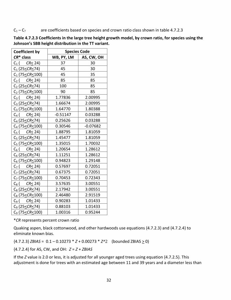
32

C1 – C7 are coefficients based on species and crown ratio class shown in table 4.7.2.3

Table 4.7.2.3 Coefficients in the large tree height growth model, by crown ratio, for species using the Johnson’s SBB height distribution in the TT variant.

Coefficient by CR* class

Species Code WB, PY, LM AS, CW, OH

C1 ( CR< 24) 37 30 C1 (25<CR<74) 45 30 C1 (75<CR<100) 45 35 C2 ( CR< 24) 85 85 C2 (25<CR<74) 100 85 C2 (75<CR<100) 90 85 C3 ( CR< 24) 1.77836 2.00995 C3 (25<CR<74) 1.66674 2.00995 C3 (75<CR<100) 1.64770 1.80388 C4 ( CR< 24) -0.51147 0.03288 C4 (25<CR<74) 0.25626 0.03288 C4 (75<CR<100) 0.30546 -0.07682 C5 ( CR< 24) 1.88795 1.81059 C5 (25<CR<74) 1.45477 1.81059 C5 (75<CR<100) 1.35015 1.70032 C6 ( CR< 24) 1.20654 1.28612 C6 (25<CR<74) 1.11251 1.28612 C6 (75<CR<100) 0.94823 1.29148 C7 ( CR< 24) 0.57697 0.72051 C7 (25<CR<74) 0.67375 0.72051 C7 (75<CR<100) 0.70453 0.72343 C8 ( CR< 24) 3.57635 3.00551 C8 (25<CR<74) 2.17942 3.00551 C8 (75<CR<100) 2.46480 2.91519 C9 ( CR< 24) 0.90283 1.01433 C9 (25<CR<74) 0.88103 1.01433 C9 (75<CR<100) 1.00316 0.95244

*CR represents percent crown ratio

Quaking aspen, black cottonwood, and other hardwoods use equations {4.7.2.3} and {4.7.2.4} to eliminate known bias.

{4.7.2.3} ZBIAS = 0.1 – 0.10273 * Z + 0.00273 * Z^2 (bounded ZBIAS > 0)

{4.7.2.4} for AS, CW, and OH: Z = Z + ZBIAS

If the Z value is 2.0 or less, it is adjusted for all younger aged trees using equation {4.7.2.5}. This adjustment is done for trees with an estimated age between 11 and 39 years and a diameter less than

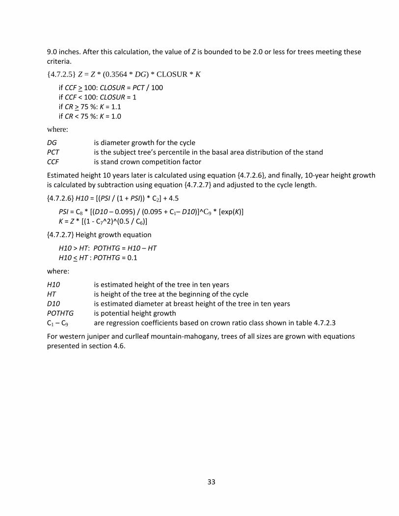
33

9.0 inches. After this calculation, the value of Z is bounded to be 2.0 or less for trees meeting these criteria.

{4.7.2.5} Z = Z * (0.3564 * DG) * CLOSUR * K

if CCF > 100: CLOSUR = PCT / 100 if CCF < 100: CLOSUR = 1 if CR > 75 %: K = 1.1 if CR < 75 %: K = 1.0

where:

DG is diameter growth for the cycle PCT is the subject tree’s percentile in the basal area distribution of the stand CCF is stand crown competition factor

Estimated height 10 years later is calculated using equation {4.7.2.6}, and finally, 10-year height growth is calculated by subtraction using equation {4.7.2.7} and adjusted to the cycle length.

{4.7.2.6} H10 = [(PSI / (1 + PSI)) * C2] + 4.5

PSI = C8 * [(D10 – 0.095) / (0.095 + C1– D10)]^C9 * [exp(K)] K = Z * [(1 - C7^2)^(0.5 / C6)]

{4.7.2.7} Height growth equation

H10 > HT: POTHTG = H10 – HT H10 < HT : POTHTG = 0.1

where:

H10 is estimated height of the tree in ten years HT is height of the tree at the beginning of the cycle D10 is estimated diameter at breast height of the tree in ten years POTHTG is potential height growth C1 – C9 are regression coefficients based on crown ratio class shown in table 4.7.2.3

For western juniper and curlleaf mountain-mahogany, trees of all sizes are grown with equations presented in section 4.6.

34

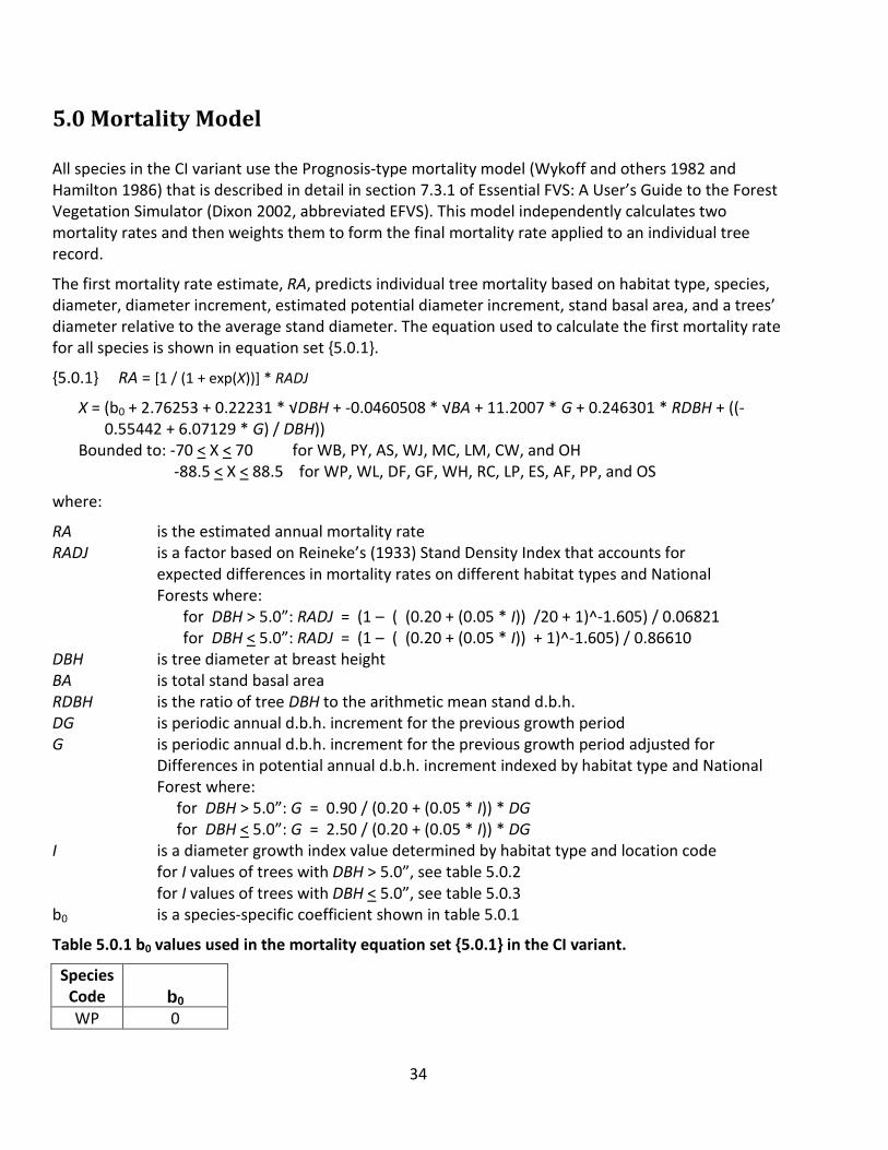
5.0 Mortality Model

All species in the CI variant use the Prognosis-type mortality model (Wykoff and others 1982 and Hamilton 1986) that is described in detail in section 7.3.1 of Essential FVS: A User’s Guide to the Forest Vegetation Simulator (Dixon 2002, abbreviated EFVS). This model independently calculates two mortality rates and then weights them to form the final mortality rate applied to an individual tree record.

The first mortality rate estimate, RA, predicts individual tree mortality based on habitat type, species, diameter, diameter increment, estimated potential diameter increment, stand basal area, and a trees’ diameter relative to the average stand diameter. The equation used to calculate the first mortality rate for all species is shown in equation set {5.0.1}.

{5.0.1} RA = [1 / (1 + exp(X))] * RADJ

X = (b0 + 2.76253 + 0.22231 * √DBH + -0.0460508 * √BA + 11.2007 * G + 0.246301 * RDBH + ((-0.55442 + 6.07129 * G) / DBH))

Bounded to: -70 < X < 70 for WB, PY, AS, WJ, MC, LM, CW, and OH -88.5 < X < 88.5 for WP, WL, DF, GF, WH, RC, LP, ES, AF, PP, and OS

where:

RA is the estimated annual mortality rate RADJ is a factor based on Reineke’s (1933) Stand Density Index that accounts for

expected differences in mortality rates on different habitat types and National Forests where:

for DBH > 5.0”: RADJ = (1 – ( (0.20 + (0.05 * I)) /20 + 1)^-1.605) / 0.06821 for DBH < 5.0”: RADJ = (1 – ( (0.20 + (0.05 * I)) + 1)^-1.605) / 0.86610

DBH is tree diameter at breast height BA is total stand basal area RDBH is the ratio of tree DBH to the arithmetic mean stand d.b.h. DG is periodic annual d.b.h. increment for the previous growth period G is periodic annual d.b.h. increment for the previous growth period adjusted for

Differences in potential annual d.b.h. increment indexed by habitat type and National Forest where:

for DBH > 5.0”: G = 0.90 / (0.20 + (0.05 * I)) * DG for DBH < 5.0”: G = 2.50 / (0.20 + (0.05 * I)) * DG

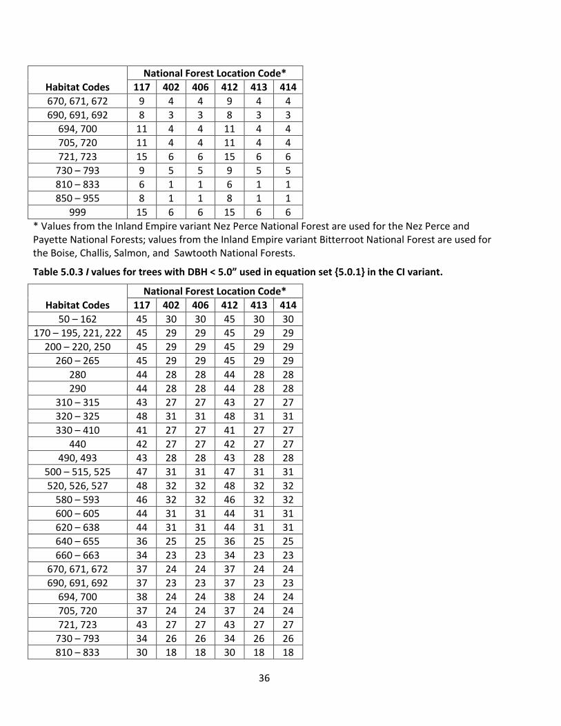
I is a diameter growth index value determined by habitat type and location code for I values of trees with DBH > 5.0”, see table 5.0.2 for I values of trees with DBH < 5.0”, see table 5.0.3 b0 is a species-specific coefficient shown in table 5.0.1

Table 5.0.1 b0 values used in the mortality equation set {5.0.1} in the CI variant.

Species Code b0 WP 0

35

Species Code b0 WL -0.17603 DF 0.317888 GF 0.317888 WH 0.607725 RC 1.57976 LP -0.12057 ES 0.94019 AF 0.21180 PP 0.21180 WB 0 PY 0 AS 0 WJ 0 MC 0 LM 0 CW 0 OS 0 OH 0

Table 5.0.2 I values for trees with DBH > 5.0” used in equation set {5.0.1} in the CI variant.

Habitat Codes National Forest Location Code*

117 402 406 412 413 414 50 – 162 15 7 7 15 7 7

170 – 195, 221, 222 15 6 6 15 6 6 200 – 220, 250 15 6 6 15 6 6

260 – 265 15 6 6 15 6 6 280 14 6 6 14 6 6 290 14 6 6 14 6 6

310 – 315 9 5 5 9 5 5 320 – 325 13 6 6 13 6 6 330 – 410 13 5 5 13 5 5

440 14 6 6 14 6 6 490, 493 14 6 6 14 6 6

500 – 515, 525 13 6 6 13 6 6 520, 526, 527 14 6 6 14 6 6

580 – 593 14 7 7 14 7 7 600 – 605 14 7 7 14 7 7 620 – 638 14 7 7 14 7 7 640 – 655 10 5 5 10 5 5 660 – 663 9 3 3 9 3 3

36


117 402 406 412 413 414 670, 671, 672 9 4 4 9 4 4 690, 691, 692 8 3 3 8 3 3

694, 700 11 4 4 11 4 4 705, 720 11 4 4 11 4 4 721, 723 15 6 6 15 6 6

730 – 793 9 5 5 9 5 5 810 – 833 6 1 1 6 1 1 850 – 955 8 1 1 8 1 1

999 15 6 6 15 6 6 * Values from the Inland Empire variant Nez Perce National Forest are used for the Nez Perce and Payette National Forests; values from the Inland Empire variant Bitterroot National Forest are used for the Boise, Challis, Salmon, and Sawtooth National Forests.

Table 5.0.3 I values for trees with DBH < 5.0” used in equation set {5.0.1} in the CI variant.


117 402 406 412 413 414 50 – 162 45 30 30 45 30 30

170 – 195, 221, 222 45 29 29 45 29 29 200 – 220, 250 45 29 29 45 29 29

260 – 265 45 29 29 45 29 29 280 44 28 28 44 28 28 290 44 28 28 44 28 28

310 – 315 43 27 27 43 27 27 320 – 325 48 31 31 48 31 31 330 – 410 41 27 27 41 27 27

440 42 27 27 42 27 27 490, 493 43 28 28 43 28 28

500 – 515, 525 47 31 31 47 31 31 520, 526, 527 48 32 32 48 32 32

580 – 593 46 32 32 46 32 32 600 – 605 44 31 31 44 31 31 620 – 638 44 31 31 44 31 31 640 – 655 36 25 25 36 25 25 660 – 663 34 23 23 34 23 23

670, 671, 672 37 24 24 37 24 24 690, 691, 692 37 23 23 37 23 23

694, 700 38 24 24 38 24 24 705, 720 37 24 24 37 24 24 721, 723 43 27 27 43 27 27

730 – 793 34 26 26 34 26 26 810 – 833 30 18 18 30 18 18

37


117 402 406 412 413 414 850 – 955 33 16 16 33 16 16

999 43 27 27 43 27 27 * Values from the Inland Empire variant Nez Perce National Forest are used for the Nez Perce and Payette National Forests; values from the Inland Empire variant Bitterroot National Forest are used for the Boise, Challis, Salmon, and Sawtooth National Forests.

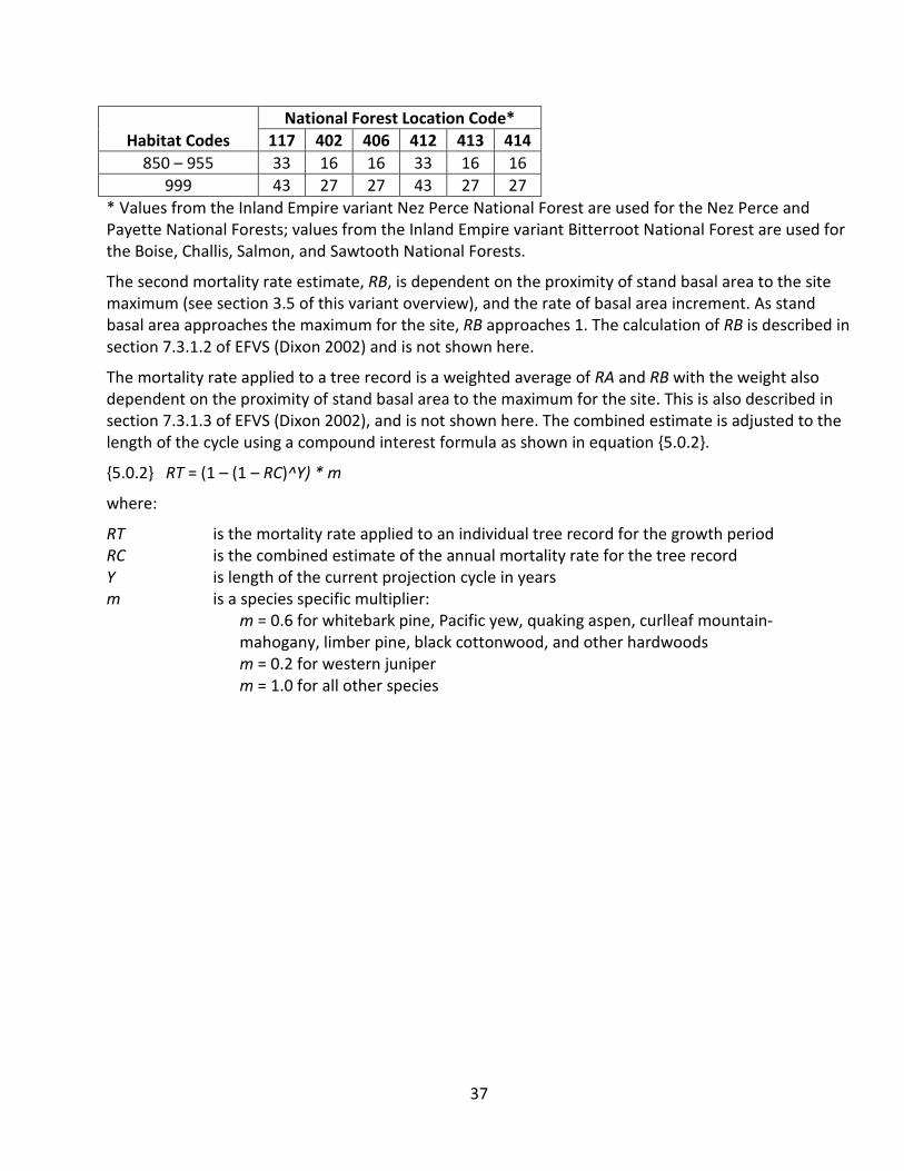
The second mortality rate estimate, RB, is dependent on the proximity of stand basal area to the site maximum (see section 3.5 of this variant overview), and the rate of basal area increment. As stand basal area approaches the maximum for the site, RB approaches 1. The calculation of RB is described in section 7.3.1.2 of EFVS (Dixon 2002) and is not shown here.

The mortality rate applied to a tree record is a weighted average of RA and RB with the weight also dependent on the proximity of stand basal area to the maximum for the site. This is also described in section 7.3.1.3 of EFVS (Dixon 2002), and is not shown here. The combined estimate is adjusted to the length of the cycle using a compound interest formula as shown in equation {5.0.2}.

{5.0.2} RT = (1 – (1 – RC)^Y) * m

where:

RT is the mortality rate applied to an individual tree record for the growth period RC is the combined estimate of the annual mortality rate for the tree record Y is length of the current projection cycle in years m is a species specific multiplier:

m = 0.6 for whitebark pine, Pacific yew, quaking aspen, curlleaf mountain-mahogany, limber pine, black cottonwood, and other hardwoods

m = 0.2 for western juniper m = 1.0 for all other species

38

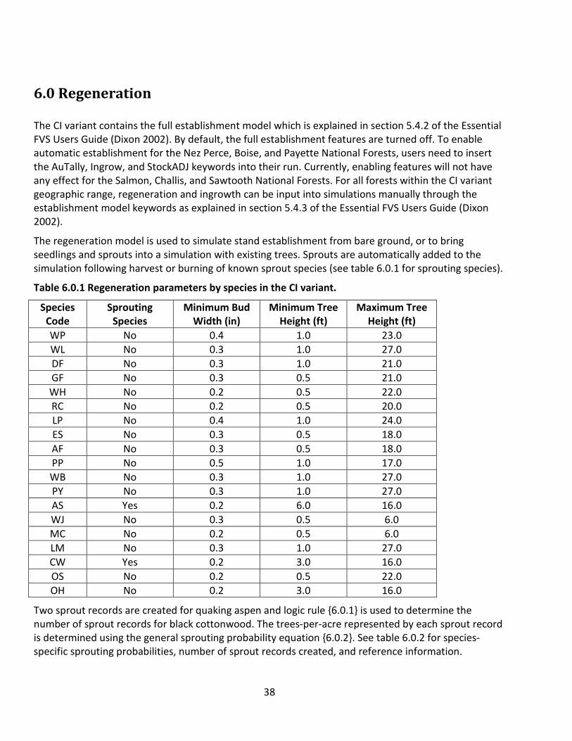
6.0 Regeneration

The CI variant contains the full establishment model which is explained in section 5.4.2 of the Essential FVS Users Guide (Dixon 2002). By default, the full establishment features are turned off. To enable automatic establishment for the Nez Perce, Boise, and Payette National Forests, users need to insert the AuTally, Ingrow, and StockADJ keywords into their run. Currently, enabling features will not have any effect for the Salmon, Challis, and Sawtooth National Forests. For all forests within the CI variant geographic range, regeneration and ingrowth can be input into simulations manually through the establishment model keywords as explained in section 5.4.3 of the Essential FVS Users Guide (Dixon 2002).

The regeneration model is used to simulate stand establishment from bare ground, or to bring seedlings and sprouts into a simulation with existing trees. Sprouts are automatically added to the simulation following harvest or burning of known sprout species (see table 6.0.1 for sprouting species).

Table 6.0.1 Regeneration parameters by species in the CI variant.

Species Code

Sprouting Species

Minimum Bud Width (in)

Minimum Tree Height (ft)

Maximum Tree Height (ft)

WP No 0.4 1.0 23.0 WL No 0.3 1.0 27.0 DF No 0.3 1.0 21.0 GF No 0.3 0.5 21.0 WH No 0.2 0.5 22.0 RC No 0.2 0.5 20.0 LP No 0.4 1.0 24.0 ES No 0.3 0.5 18.0 AF No 0.3 0.5 18.0 PP No 0.5 1.0 17.0 WB No 0.3 1.0 27.0 PY No 0.3 1.0 27.0 AS Yes 0.2 6.0 16.0 WJ No 0.3 0.5 6.0 MC No 0.2 0.5 6.0 LM No 0.3 1.0 27.0 CW Yes 0.2 3.0 16.0 OS No 0.2 0.5 22.0 OH No 0.2 3.0 16.0

Two sprout records are created for quaking aspen and logic rule {6.0.1} is used to determine the number of sprout records for black cottonwood. The trees-per-acre represented by each sprout record is determined using the general sprouting probability equation {6.0.2}. See table 6.0.2 for species-specific sprouting probabilities, number of sprout records created, and reference information.

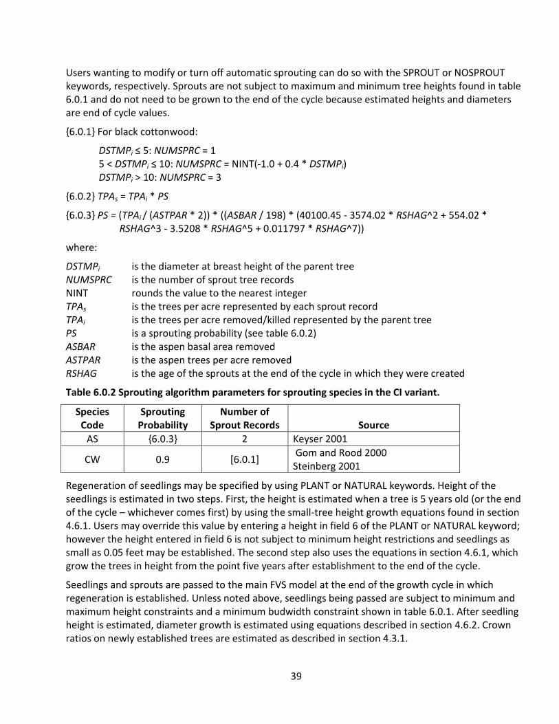
39

Users wanting to modify or turn off automatic sprouting can do so with the SPROUT or NOSPROUT keywords, respectively. Sprouts are not subject to maximum and minimum tree heights found in table 6.0.1 and do not need to be grown to the end of the cycle because estimated heights and diameters are end of cycle values.

{6.0.1} For black cottonwood:

DSTMPi ≤ 5: NUMSPRC = 1 5 < DSTMPi ≤ 10: NUMSPRC = NINT(-1.0 + 0.4 * DSTMPi)

DSTMPi > 10: NUMSPRC = 3

{6.0.2} TPAs = TPAi * PS

{6.0.3} PS = (TPAi / (ASTPAR * 2)) * ((ASBAR / 198) * (40100.45 - 3574.02 * RSHAG^2 + 554.02 * RSHAG^3 - 3.5208 * RSHAG^5 + 0.011797 * RSHAG^7))

where:

DSTMPi is the diameter at breast height of the parent tree NUMSPRC is the number of sprout tree records NINT rounds the value to the nearest integer TPAs is the trees per acre represented by each sprout record TPAi is the trees per acre removed/killed represented by the parent tree PS is a sprouting probability (see table 6.0.2) ASBAR is the aspen basal area removed ASTPAR is the aspen trees per acre removed RSHAG is the age of the sprouts at the end of the cycle in which they were created

Table 6.0.2 Sprouting algorithm parameters for sprouting species in the CI variant.

Species Code

Sprouting Probability

Number of Sprout Records Source

AS {6.0.3} 2 Keyser 2001

CW 0.9 [6.0.1] Gom and Rood 2000 Steinberg 2001

Regeneration of seedlings may be specified by using PLANT or NATURAL keywords. Height of the seedlings is estimated in two steps. First, the height is estimated when a tree is 5 years old (or the end of the cycle – whichever comes first) by using the small-tree height growth equations found in section 4.6.1. Users may override this value by entering a height in field 6 of the PLANT or NATURAL keyword; however the height entered in field 6 is not subject to minimum height restrictions and seedlings as small as 0.05 feet may be established. The second step also uses the equations in section 4.6.1, which grow the trees in height from the point five years after establishment to the end of the cycle.

Seedlings and sprouts are passed to the main FVS model at the end of the growth cycle in which regeneration is established. Unless noted above, seedlings being passed are subject to minimum and maximum height constraints and a minimum budwidth constraint shown in table 6.0.1. After seedling height is estimated, diameter growth is estimated using equations described in section 4.6.2. Crown ratios on newly established trees are estimated as described in section 4.3.1.

40

Regenerated trees and sprouts can be identified in the treelist output file with tree identification numbers beginning with the letters “ES”.

41

7.0 Volume

Volume is calculated for three merchantability standards: total stem cubic feet, merchantable stem cubic feet, and merchantable stem board feet (Scribner Decimal C). Volume estimation is based on methods contained in the National Volume Estimator Library maintained by the Forest Products Measurements group in the Forest Management Service Center (Volume Estimator Library Equations 2009). The default merchantability standards and equation numbers for the CI variant are shown in tables 7.0.1 – 7.0.3.

Table 7.0.1 Default volume merchantability standards for the CI variant.

Merchantable Cubic Foot Volume Specifications: Minimum DBH / Top Diameter LP All Other Species All location codes 7.0 / 6.0 inches 8.0 / 6.0 inches Stump Height 1.0 foot 1.0 foot Merchantable Board Foot Volume Specifications: Minimum DBH / Top Diameter LP All Other Species All location codes 7.0 / 6.0 inches 8.0 / 6.0 inches Stump Height 1.0 foot 1.0 foot

Table 7.0.2 Volume equation defaults for each species, at specific location codes, with model name.

Common Name Location Code Equation Number Reference western white pine 117 I00FW2W119 Flewelling's 2-Point Profile Model western white pine All Region 4 codes 400MATW117 Rustagi and Loveless Profile Model

western larch 117 I00FW2W073 Flewelling's 2-Point Profile Model western larch All Region 4 codes 400MATW073 Rustagi and Loveless Profile Model

Douglas-fir 117 I00FW2W202 Flewelling's 2-Point Profile Model Douglas-fir 402, 412, 413 I15FW2W202 Flewelling's 2-Point Profile Model Douglas-fir 406, 414 400MATW202 Rustagi and Loveless Profile Model

grand fir 117 I00FW2W017 Flewelling's 2-Point Profile Model grand fir 402, 412, 413 I15FW2W017 Flewelling's 2-Point Profile Model grand fir 406, 414 400MATW015 Rustagi and Loveless Profile Model

western hemlock 117 I00FW2W260 Flewelling's 2-Point Profile Model western hemlock All Region 4 codes 400MATW015 Rustagi and Loveless Profile Model western redcedar 117 I00FW2W242 Flewelling's 2-Point Profile Model western redcedar All Region 4 codes 400MATW081 Rustagi and Loveless Profile Model

lodgepole pine 117 I00FW2W108 Flewelling's 2-Point Profile Model lodgepole pine All Region 4 codes 400MATW108 Rustagi and Loveless Profile Model

Engelmann spruce 117 I00FW2W093 Flewelling's 2-Point Profile Model Engelmann spruce 402, 412, 413 I15FW2W093 Flewelling's 2-Point Profile Model Engelmann spruce 406, 414 400MATW093 Rustagi and Loveless Profile Model

subalpine fir 117 I00FW2W019 Flewelling's 2-Point Profile Model subalpine fir All Region 4 codes 400MATW019 Rustagi and Loveless Profile Model

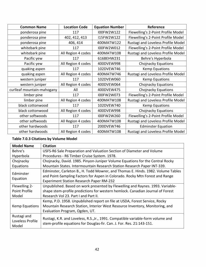
42

Common Name Location Code Equation Number Reference ponderosa pine 117 I00FW2W122 Flewelling's 2-Point Profile Model ponderosa pine 402, 412, 413 I15FW2W122 Flewelling's 2-Point Profile Model ponderosa pine 406, 414 400MATW122 Rustagi and Loveless Profile Model whitebark pine 117 I00FW2W012 Flewelling's 2-Point Profile Model whitebark pine All Region 4 codes 400MATW108 Rustagi and Loveless Profile Model

Pacific yew 117 616BEHW231 Behre's Hyperbola Pacific yew All Region 4 codes 400DVEW998 Chojnacky Equations

quaking aspen 117 102DVEW746 Kemp Equations quaking aspen All Region 4 codes 400MATW746 Rustagi and Loveless Profile Model

western juniper 117 102DVEW060 Kemp Equations western juniper All Region 4 codes 400DVEW064 Chojnacky Equations

curlleaf mountain-mahogany All 400DVEW475 Chojnacky Equations limber pine 117 I00FW2W073 Flewelling's 2-Point Profile Model limber pine All Region 4 codes 400MATW108 Rustagi and Loveless Profile Model

black cottonwood 117 102DVEW740 Kemp Equations black cottonwood All Region 4 codes 400DVEW998 Chojnacky Equations other softwoods 117 I00FW2W260 Flewelling's 2-Point Profile Model other softwoods All Region 4 codes 400MATW108 Rustagi and Loveless Profile Model other hardwoods 117 200DVEW746 Edminster Equation other hardwoods All Region 4 codes 400MATW108 Rustagi and Loveless Profile Model

Table 7.0.3 Citations by Volume Model

Model Name Citation Behre's Hyperbola

USFS-R6 Sale Preparation and Valuation Section of Diameter and Volume Procedures - R6 Timber Cruise System. 1978.

Chojnacky Equations

Chojnacky, David. 1985. Pinyon-Juniper Volume Equations for the Central Rocky Mountain States. Intermountain Research Station Research Paper INT-339.

Edminster Equation

Edminster, Carleton B., H. Todd Mowrer, and Thomas E. Hinds. 1982. Volume Tables and Point-Sampling Factors for Aspen in Colorado. Rocky Mtn Forest and Range Experiment Station Research Paper RM-232

Flewelling 2-Point Profile Model

Unpublished. Based on work presented by Flewelling and Raynes. 1993. Variable-shape stem-profile predictions for western hemlock. Canadian Journal of Forest Research Vol 23. Part I and Part II.

Kemp Equations Kemp, P.D. 1958. Unpublished report on file at USDA, Forest Service, Rocky Mountain Research Station, Interior West Resource Inventory, Monitoring, and Evaluation Program, Ogden, UT.

Rustagi and Loveless Profile Model

Rustagi, K.R. and Loveless, R.S.,Jr., 1991. Compatible variable-form volume and stem-profile equations for Douglas-fir. Can. J. For. Res. 21:143-151.

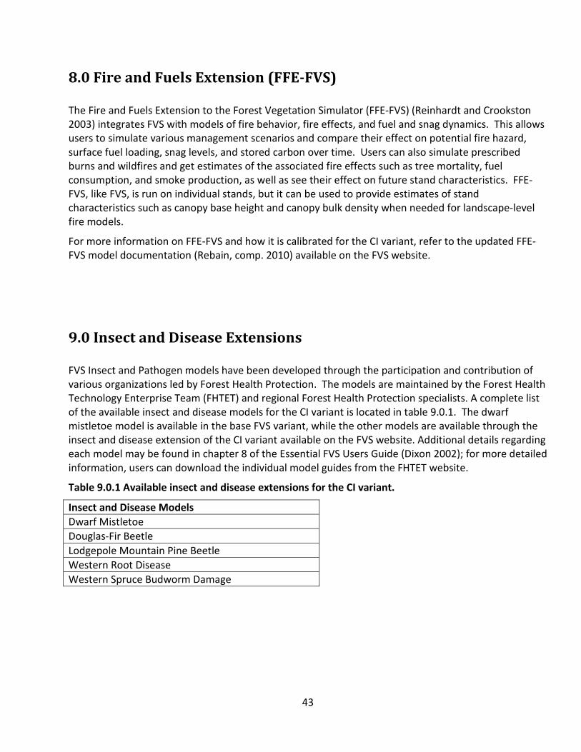
43

8.0 Fire and Fuels Extension (FFE-FVS)

The Fire and Fuels Extension to the Forest Vegetation Simulator (FFE-FVS) (Reinhardt and Crookston 2003) integrates FVS with models of fire behavior, fire effects, and fuel and snag dynamics. This allows users to simulate various management scenarios and compare their effect on potential fire hazard, surface fuel loading, snag levels, and stored carbon over time. Users can also simulate prescribed burns and wildfires and get estimates of the associated fire effects such as tree mortality, fuel consumption, and smoke production, as well as see their effect on future stand characteristics. FFE-FVS, like FVS, is run on individual stands, but it can be used to provide estimates of stand characteristics such as canopy base height and canopy bulk density when needed for landscape-level fire models.

For more information on FFE-FVS and how it is calibrated for the CI variant, refer to the updated FFE-FVS model documentation (Rebain, comp. 2010) available on the FVS website.

9.0 Insect and Disease Extensions

FVS Insect and Pathogen models have been developed through the participation and contribution of various organizations led by Forest Health Protection. The models are maintained by the Forest Health Technology Enterprise Team (FHTET) and regional Forest Health Protection specialists. A complete list of the available insect and disease models for the CI variant is located in table 9.0.1. The dwarf mistletoe model is available in the base FVS variant, while the other models are available through the insect and disease extension of the CI variant available on the FVS website. Additional details regarding each model may be found in chapter 8 of the Essential FVS Users Guide (Dixon 2002); for more detailed information, users can download the individual model guides from the FHTET website.

Table 9.0.1 Available insect and disease extensions for the CI variant.

Insect and Disease Models Dwarf Mistletoe Douglas-Fir Beetle Lodgepole Mountain Pine Beetle Western Root Disease Western Spruce Budworm Damage

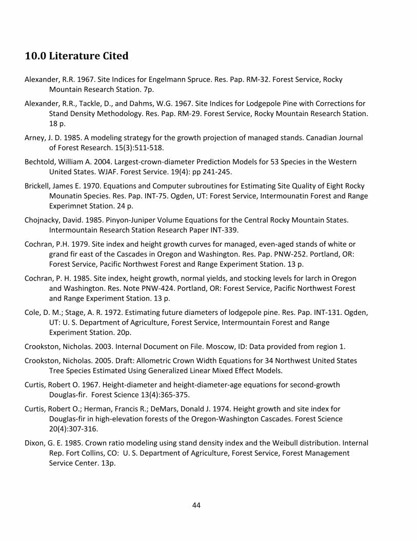
44

10.0 Literature Cited

Alexander, R.R. 1967. Site Indices for Engelmann Spruce. Res. Pap. RM-32. Forest Service, Rocky Mountain Research Station. 7p.

Alexander, R.R., Tackle, D., and Dahms, W.G. 1967. Site Indices for Lodgepole Pine with Corrections for Stand Density Methodology. Res. Pap. RM-29. Forest Service, Rocky Mountain Research Station. 18 p.

Arney, J. D. 1985. A modeling strategy for the growth projection of managed stands. Canadian Journal of Forest Research. 15(3):511-518.

Bechtold, William A. 2004. Largest-crown-diameter Prediction Models for 53 Species in the Western United States. WJAF. Forest Service. 19(4): pp 241-245.

Brickell, James E. 1970. Equations and Computer subroutines for Estimating Site Quality of Eight Rocky Mounatin Species. Res. Pap. INT-75. Ogden, UT: Forest Service, Intermounatin Forest and Range Experimnet Station. 24 p.

Chojnacky, David. 1985. Pinyon-Juniper Volume Equations for the Central Rocky Mountain States. Intermountain Research Station Research Paper INT-339.

Cochran, P.H. 1979. Site index and height growth curves for managed, even-aged stands of white or grand fir east of the Cascades in Oregon and Washington. Res. Pap. PNW-252. Portland, OR: Forest Service, Pacific Northwest Forest and Range Experiment Station. 13 p.

Cochran, P. H. 1985. Site index, height growth, normal yields, and stocking levels for larch in Oregon and Washington. Res. Note PNW-424. Portland, OR: Forest Service, Pacific Northwest Forest and Range Experiment Station. 13 p.

Cole, D. M.; Stage, A. R. 1972. Estimating future diameters of lodgepole pine. Res. Pap. INT-131. Ogden, UT: U. S. Department of Agriculture, Forest Service, Intermountain Forest and Range Experiment Station. 20p.

Crookston, Nicholas. 2003. Internal Document on File. Moscow, ID: Data provided from region 1.

Crookston, Nicholas. 2005. Draft: Allometric Crown Width Equations for 34 Northwest United States Tree Species Estimated Using Generalized Linear Mixed Effect Models.

Curtis, Robert O. 1967. Height-diameter and height-diameter-age equations for second-growth Douglas-fir. Forest Science 13(4):365-375.

Curtis, Robert O.; Herman, Francis R.; DeMars, Donald J. 1974. Height growth and site index for Douglas-fir in high-elevation forests of the Oregon-Washington Cascades. Forest Science 20(4):307-316.

Dixon, G. E. 1985. Crown ratio modeling using stand density index and the Weibull distribution. Internal Rep. Fort Collins, CO: U. S. Department of Agriculture, Forest Service, Forest Management Service Center. 13p.

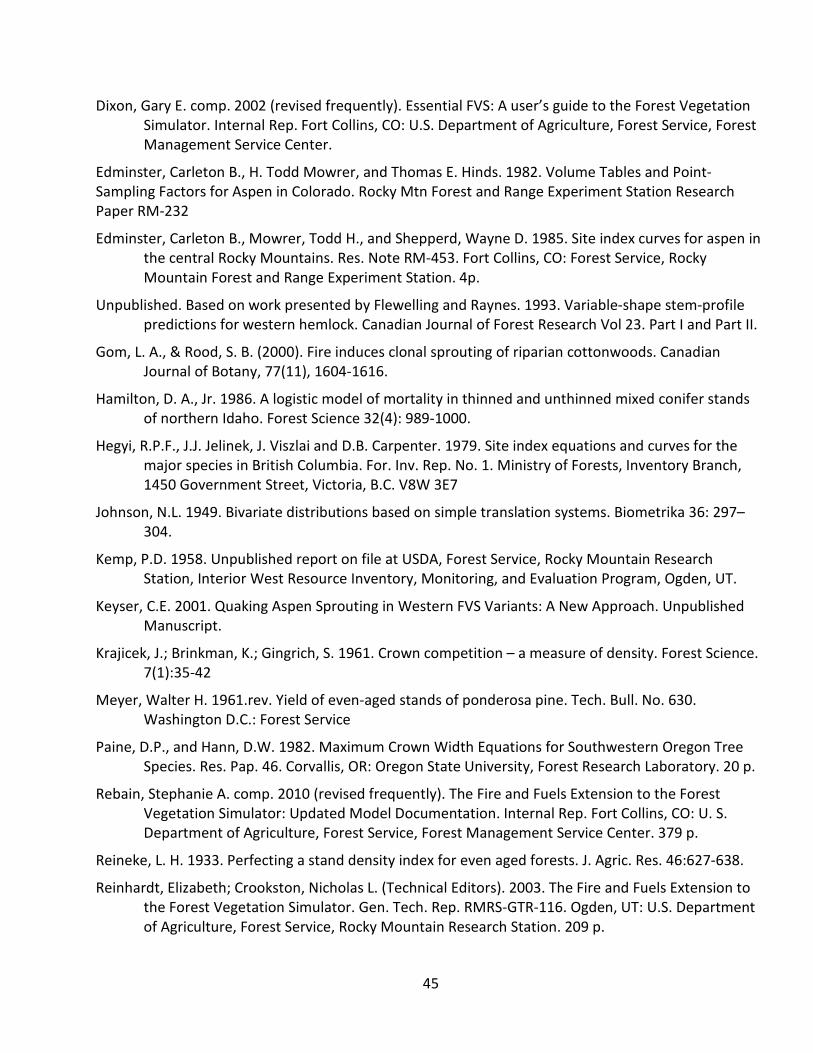
45

Dixon, Gary E. comp. 2002 (revised frequently). Essential FVS: A user’s guide to the Forest Vegetation Simulator. Internal Rep. Fort Collins, CO: U.S. Department of Agriculture, Forest Service, Forest Management Service Center.

Edminster, Carleton B., H. Todd Mowrer, and Thomas E. Hinds. 1982. Volume Tables and Point-Sampling Factors for Aspen in Colorado. Rocky Mtn Forest and Range Experiment Station Research Paper RM-232

Edminster, Carleton B., Mowrer, Todd H., and Shepperd, Wayne D. 1985. Site index curves for aspen in the central Rocky Mountains. Res. Note RM-453. Fort Collins, CO: Forest Service, Rocky Mountain Forest and Range Experiment Station. 4p.

Unpublished. Based on work presented by Flewelling and Raynes. 1993. Variable-shape stem-profile predictions for western hemlock. Canadian Journal of Forest Research Vol 23. Part I and Part II.

Gom, L. A., & Rood, S. B. (2000). Fire induces clonal sprouting of riparian cottonwoods. Canadian Journal of Botany, 77(11), 1604-1616.

Hamilton, D. A., Jr. 1986. A logistic model of mortality in thinned and unthinned mixed conifer stands of northern Idaho. Forest Science 32(4): 989-1000.

Hegyi, R.P.F., J.J. Jelinek, J. Viszlai and D.B. Carpenter. 1979. Site index equations and curves for the major species in British Columbia. For. Inv. Rep. No. 1. Ministry of Forests, Inventory Branch, 1450 Government Street, Victoria, B.C. V8W 3E7

Johnson, N.L. 1949. Bivariate distributions based on simple translation systems. Biometrika 36: 297–304.

Kemp, P.D. 1958. Unpublished report on file at USDA, Forest Service, Rocky Mountain Research Station, Interior West Resource Inventory, Monitoring, and Evaluation Program, Ogden, UT.

Keyser, C.E. 2001. Quaking Aspen Sprouting in Western FVS Variants: A New Approach. Unpublished Manuscript.

Krajicek, J.; Brinkman, K.; Gingrich, S. 1961. Crown competition – a measure of density. Forest Science. 7(1):35-42

Meyer, Walter H. 1961.rev. Yield of even-aged stands of ponderosa pine. Tech. Bull. No. 630. Washington D.C.: Forest Service

Paine, D.P., and Hann, D.W. 1982. Maximum Crown Width Equations for Southwestern Oregon Tree Species. Res. Pap. 46. Corvallis, OR: Oregon State University, Forest Research Laboratory. 20 p.

Rebain, Stephanie A. comp. 2010 (revised frequently). The Fire and Fuels Extension to the Forest Vegetation Simulator: Updated Model Documentation. Internal Rep. Fort Collins, CO: U. S. Department of Agriculture, Forest Service, Forest Management Service Center. 379 p.

Reineke, L. H. 1933. Perfecting a stand density index for even aged forests. J. Agric. Res. 46:627-638.

Reinhardt, Elizabeth; Crookston, Nicholas L. (Technical Editors). 2003. The Fire and Fuels Extension to the Forest Vegetation Simulator. Gen. Tech. Rep. RMRS-GTR-116. Ogden, UT: U.S. Department of Agriculture, Forest Service, Rocky Mountain Research Station. 209 p.

46

Rustagi, K.R. and Loveless, R.S.,Jr., 1991. Compatible variable-form volume and stem-profile equations for Douglas-fir. Can. J. For. Res. 21:143-151.

Schreuder, H.T. and W.L. Hafley. 1977. A Useful Distribution for Describing Stand Structure of Tree Heights and Diameters. Biometrics 33, 471-478.

Shepperd, Wayne D. 1995. Unpublished equation. Data on file. Fort Collins, CO: Forest Service, Rocky Mountain Research Station.

Stage, A. R. 1973. Prognosis Model for stand development. Res. Paper INT-137. Ogden, UT: U. S. Department of Agriculture, Forest Service, Intermountain Forest and Range Experiment Station. 32p.

Steinberg, Peter D. 2001. Populus balsamifera subsp. trichocarpa. In: Fire Effects Information System, [Online]. U.S. Department of Agriculture, Forest Service, Rocky Mountain Research Station, Fire Sciences Laboratory (Producer).

USFS-R6 Sale Preparation and Valuation Section of Diameter and Volume Procedures - R6 Timber Cruise System. 1978.

Van Dyck, Michael G.; Smith-Mateja, Erin E., comps. 2000 (revised frequently). Keyword reference guide for the Forest Vegetation Simulator. Internal Rep. Fort Collins, CO: U. S. Department of Agriculture, Forest Service, Forest Management Service Center.

Wiley, Kenneth N. 1978. Site index tables for western hemlock in the Pacific Northwest. For. Pap. No. 17. Centralia, WA: Weyerhaeuser Forestry Research Center. 28 p.

Wykoff, W. R. 1990. A basal area increment model for individual conifers in the northern Rocky Mountains. For. Science 36(4): 1077-1104.

Wykoff, William R., Crookston, Nicholas L., and Stage, Albert R. 1982. User’s guide to the Stand Prognosis Model. Gen. Tech. Rep. INT-133. Ogden, UT: Forest Service, Intermountain Forest and Range Experiment Station. 112p.

-----. 2009(revised frequently). Volume Estimator Library Equations. Internal Rep. Fort Collins, CO: U. S. Department of Agriculture, Forest Service, Forest Management Service Center.

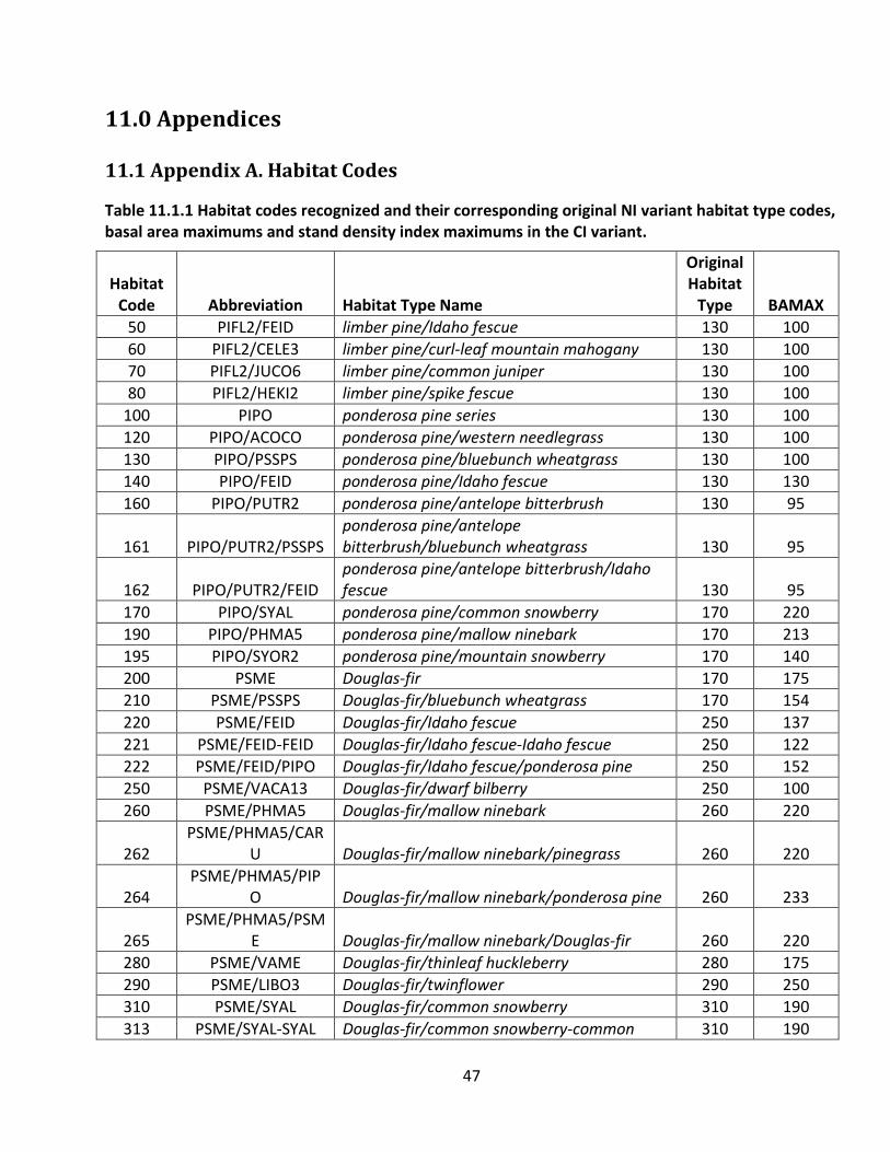
47

11.0 Appendices

11.1 Appendix A. Habitat Codes

Table 11.1.1 Habitat codes recognized and their corresponding original NI variant habitat type codes, basal area maximums and stand density index maximums in the CI variant.

Habitat Code Abbreviation Habitat Type Name

Original Habitat

Type BAMAX 50 PIFL2/FEID limber pine/Idaho fescue 130 100 60 PIFL2/CELE3 limber pine/curl-leaf mountain mahogany 130 100 70 PIFL2/JUCO6 limber pine/common juniper 130 100 80 PIFL2/HEKI2 limber pine/spike fescue 130 100

100 PIPO ponderosa pine series 130 100 120 PIPO/ACOCO ponderosa pine/western needlegrass 130 100 130 PIPO/PSSPS ponderosa pine/bluebunch wheatgrass 130 100 140 PIPO/FEID ponderosa pine/Idaho fescue 130 130 160 PIPO/PUTR2 ponderosa pine/antelope bitterbrush 130 95

161 PIPO/PUTR2/PSSPS ponderosa pine/antelope bitterbrush/bluebunch wheatgrass 130 95

162 PIPO/PUTR2/FEID ponderosa pine/antelope bitterbrush/Idaho fescue 130 95

170 PIPO/SYAL ponderosa pine/common snowberry 170 220 190 PIPO/PHMA5 ponderosa pine/mallow ninebark 170 213 195 PIPO/SYOR2 ponderosa pine/mountain snowberry 170 140 200 PSME Douglas-fir 170 175 210 PSME/PSSPS Douglas-fir/bluebunch wheatgrass 170 154 220 PSME/FEID Douglas-fir/Idaho fescue 250 137 221 PSME/FEID-FEID Douglas-fir/Idaho fescue-Idaho fescue 250 122 222 PSME/FEID/PIPO Douglas-fir/Idaho fescue/ponderosa pine 250 152 250 PSME/VACA13 Douglas-fir/dwarf bilberry 250 100 260 PSME/PHMA5 Douglas-fir/mallow ninebark 260 220

262 PSME/PHMA5/CAR

U Douglas-fir/mallow ninebark/pinegrass 260 220

264 PSME/PHMA5/PIP

O Douglas-fir/mallow ninebark/ponderosa pine 260 233

265 PSME/PHMA5/PSM

E Douglas-fir/mallow ninebark/Douglas-fir 260 220 280 PSME/VAME Douglas-fir/thinleaf huckleberry 280 175 290 PSME/LIBO3 Douglas-fir/twinflower 290 250 310 PSME/SYAL Douglas-fir/common snowberry 310 190 313 PSME/SYAL-SYAL Douglas-fir/common snowberry-common 310 190

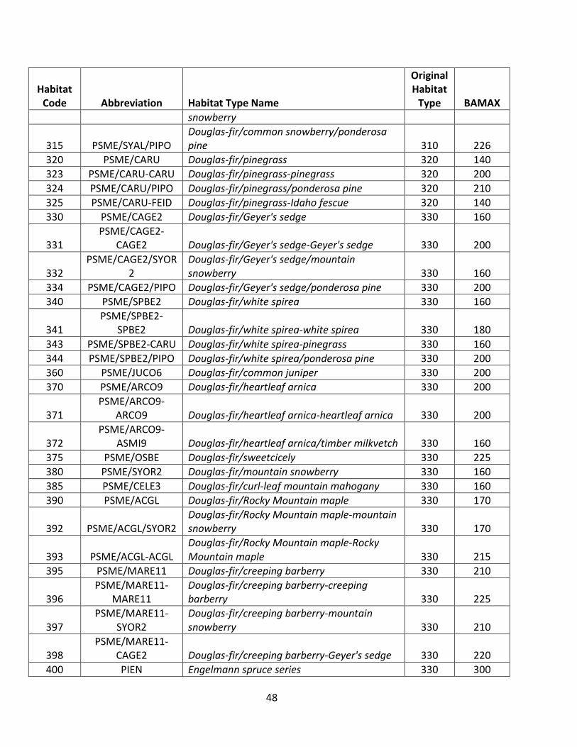
48


Original Habitat

Type BAMAX snowberry

315 PSME/SYAL/PIPO Douglas-fir/common snowberry/ponderosa pine 310 226

320 PSME/CARU Douglas-fir/pinegrass 320 140 323 PSME/CARU-CARU Douglas-fir/pinegrass-pinegrass 320 200 324 PSME/CARU/PIPO Douglas-fir/pinegrass/ponderosa pine 320 210 325 PSME/CARU-FEID Douglas-fir/pinegrass-Idaho fescue 320 140 330 PSME/CAGE2 Douglas-fir/Geyer's sedge 330 160

331 PSME/CAGE2-

CAGE2 Douglas-fir/Geyer's sedge-Geyer's sedge 330 200

332 PSME/CAGE2/SYOR

2 Douglas-fir/Geyer's sedge/mountain snowberry 330 160

334 PSME/CAGE2/PIPO Douglas-fir/Geyer's sedge/ponderosa pine 330 200 340 PSME/SPBE2 Douglas-fir/white spirea 330 160

341 PSME/SPBE2-

SPBE2 Douglas-fir/white spirea-white spirea 330 180 343 PSME/SPBE2-CARU Douglas-fir/white spirea-pinegrass 330 160 344 PSME/SPBE2/PIPO Douglas-fir/white spirea/ponderosa pine 330 200 360 PSME/JUCO6 Douglas-fir/common juniper 330 200 370 PSME/ARCO9 Douglas-fir/heartleaf arnica 330 200

371 PSME/ARCO9-

ARCO9 Douglas-fir/heartleaf arnica-heartleaf arnica 330 200

372 PSME/ARCO9-

ASMI9 Douglas-fir/heartleaf arnica/timber milkvetch 330 160 375 PSME/OSBE Douglas-fir/sweetcicely 330 225 380 PSME/SYOR2 Douglas-fir/mountain snowberry 330 160 385 PSME/CELE3 Douglas-fir/curl-leaf mountain mahogany 330 160 390 PSME/ACGL Douglas-fir/Rocky Mountain maple 330 170

392 PSME/ACGL/SYOR2 Douglas-fir/Rocky Mountain maple-mountain snowberry 330 170

393 PSME/ACGL-ACGL Douglas-fir/Rocky Mountain maple-Rocky Mountain maple 330 215

395 PSME/MARE11 Douglas-fir/creeping barberry 330 210

396 PSME/MARE11-

MARE11 Douglas-fir/creeping barberry-creeping barberry 330 225

397 PSME/MARE11-

SYOR2 Douglas-fir/creeping barberry-mountain snowberry 330 210

398 PSME/MARE11-

CAGE2 Douglas-fir/creeping barberry-Geyer's sedge 330 220 400 PIEN Engelmann spruce series 330 300

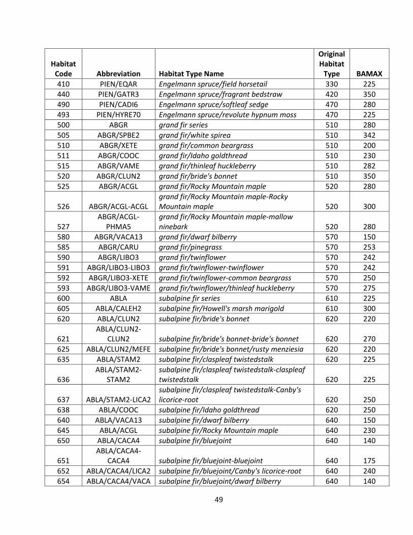
49


Original Habitat

Type BAMAX 410 PIEN/EQAR Engelmann spruce/field horsetail 330 225 440 PIEN/GATR3 Engelmann spruce/fragrant bedstraw 420 350 490 PIEN/CADI6 Engelmann spruce/softleaf sedge 470 280 493 PIEN/HYRE70 Engelmann spruce/revolute hypnum moss 470 225 500 ABGR grand fir series 510 280 505 ABGR/SPBE2 grand fir/white spirea 510 342 510 ABGR/XETE grand fir/common beargrass 510 200 511 ABGR/COOC grand fir/Idaho goldthread 510 230 515 ABGR/VAME grand fir/thinleaf huckleberry 510 282 520 ABGR/CLUN2 grand fir/bride's bonnet 510 350 525 ABGR/ACGL grand fir/Rocky Mountain maple 520 280

526 ABGR/ACGL-ACGL grand fir/Rocky Mountain maple-Rocky Mountain maple 520 300

527 ABGR/ACGL-

PHMA5 grand fir/Rocky Mountain maple-mallow ninebark 520 280

580 ABGR/VACA13 grand fir/dwarf bilberry 570 150 585 ABGR/CARU grand fir/pinegrass 570 253 590 ABGR/LIBO3 grand fir/twinflower 570 242 591 ABGR/LIBO3-LIBO3 grand fir/twinflower-twinflower 570 242 592 ABGR/LIBO3-XETE grand fir/twinflower-common beargrass 570 250 593 ABGR/LIBO3-VAME grand fir/twinflower/thinleaf huckleberry 570 275 600 ABLA subalpine fir series 610 225 605 ABLA/CALEH2 subalpine fir/Howell's marsh marigold 610 300 620 ABLA/CLUN2 subalpine fir/bride's bonnet 620 220

621 ABLA/CLUN2-

CLUN2 subalpine fir/bride's bonnet-bride's bonnet 620 270 625 ABLA/CLUN2/MEFE subalpine fir/bride's bonnet/rusty menziesia 620 220 635 ABLA/STAM2 subalpine fir/claspleaf twistedstalk 620 225

636 ABLA/STAM2-

STAM2 subalpine fir/claspleaf twistedstalk-claspleaf twistedstalk 620 225

637 ABLA/STAM2-LICA2 subalpine fir/claspleaf twistedstalk-Canby's licorice-root 620 250

638 ABLA/COOC subalpine fir/Idaho goldthread 620 250 640 ABLA/VACA13 subalpine fir/dwarf bilberry 640 150 645 ABLA/ACGL subalpine fir/Rocky Mountain maple 640 230 650 ABLA/CACA4 subalpine fir/bluejoint 640 140

651 ABLA/CACA4-

CACA4 subalpine fir/bluejoint-bluejoint 640 175 652 ABLA/CACA4/LICA2 subalpine fir/bluejoint/Canby's licorice-root 640 240 654 ABLA/CACA4/VACA subalpine fir/bluejoint/dwarf bilberry 640 140

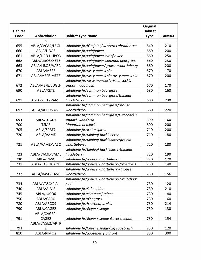
50


Original Habitat

Type BAMAX 3

655 ABLA/CACA4/LEGL subalpine fir/bluejoint/western Labrador tea 640 210 660 ABLA/LIBO3 subalpine fir/twinflower 660 200 661 ABLA/LIBO3-LIBO3 subalpine fir/twinflower-twinflower 660 250 662 ABLA/LIBO3/XETE subalpine fir/twinflower-common beargrass 660 230 663 ABLA/LIBO3/VASC subalpine fir/twinflower/grouse whortleberry 660 200 670 ABLA/MEFE subalpine fir/rusty menziesia 670 170 671 ABLA/MEFE-MEFE subalpine fir/rusty menziesia-rusty menziesia 670 200

672 ABLA/MEFE/LUGLH subalpine fir/rusty menziesia/Hitchcock's smooth woodrush 670 170

690 ABLA/XETE subalpine fir/common beargrass 680 160

691 ABLA/XETE/VAME subalpine fir/common beargrass/thinleaf huckleberry 680 230

692 ABLA/XETE/VASC subalpine fir/common beargrass/grouse whortleberry 680 220

694 ABLA/LUGLH subalpine fir/common beargrass/Hitchcock's smooth woodrush 690 160

700 TSME Mountain hemlock 690 200 705 ABLA/SPBE2 subalpine fir/white spirea 710 200 720 ABLA/VAME subalpine fir/thinleaf huckleberry 710 180

721 ABLA/VAME/VASC subalpine fir/thinleaf huckleberry/grouse whortleberry 720 180

723 ABLA/VAME-VAME subalpine fir/thinleaf huckleberry-thinleaf huckleberry 720 190

730 ABLA/VASC subalpine fir/grouse whortleberry 730 120 731 ABLA/VASC/CARU subalpine fir/grouse whortleberry/pinegrass 730 140

732 ABLA/VASC-VASC subalpine fir/grouse whortleberry-grouse whortleberry 730 156

734 ABLA/VASC/PIAL subalpine fir/grouse whortleberry/whitebark pine 730 120

740 ABLA/ALVIS subalpine fir/Sitka alder 730 210 745 ABLA/JUCO6 subalpine fir/common juniper 730 140 750 ABLA/CARU subalpine fir/pinegrass 730 160 780 ABLA/ARCO9 subalpine fir/heartleaf arnica 730 214 790 ABLA/CAGE2 subalpine fir/Geyer's sedge 730 130

791 ABLA/CAGE2-

CAGE2 subalpine fir/Geyer's sedge-Geyer's sedge 730 154

793 ABLA/CAGE2/ARTR

2 subalpine fir/Geyer's sedge/big sagebrush 730 120 810 ABLA/RIMO2 subalpine fir/gooseberry currant 830 300

51


Original Habitat

Type BAMAX 830 ABLA/LUGLH subalpine fir/Hitchcock's smooth woodrush 830 130

831 ABLA/LUGLH-VASC subalpine fir/Hitchcock's smooth woodrush/grouse whortleberry 830 130

833 ABLA/LUGLH-

LUGLH subalpine fir/Hitchcock's smooth woodrush-Hitchcock's smooth woodrush 830 200 850 PIAL-ABLA whitebark pine-subalpine fir 850 100 870 PIAL whitebark pine series 850 75 900 PICO lodgepole pine series 850 100 905 PICO-FEID lodgepole pine/Idaho fescue 850 100 920 PICO/VACA3 lodgepole pine/dwarf bilberry 850 110 940 PICO/VASC lodgepole pine/grouse whortleberry 850 150 955 PIPO/CAGE lodgepole pine/Geyer's sedge 850 150 999 OTHER 999 150

52

The U.S. Department of Agriculture (USDA) prohibits discrimination in all its programs and activities on the basis of race, color, national origin, sex, religion, age, disability, political beliefs, sexual orientation, or marital or family status. (Not all prohibited bases apply to all programs.) Persons with disabilities who require alternative means for communication of program information (Braille, large print, audiotape, etc.) should contact USDA’s TARGET Center at (202) 720-2600 (voice and TDD).

To file a complaint of discrimination, write USDA, Director, Office of Civil Rights, Room 326-W, Whitten Building, 1400 Independence Avenue, SW, Washington, DC 20250-9410 or call (202) 720-5964 (voice or TDD). USDA is an equal opportunity provider and employer.

Central Idaho (CI) Variant Overview - US Forest Service Central Idaho (CI) Variant Overview Forest...

Documents

Transcript of Central Idaho (CI) Variant Overview - US Forest Service Central Idaho (CI) Variant Overview Forest...