CASE STUDIES OF OCEAN TRANSPORTS USING THE SAFETRANS SIMULATOR · CASE STUDIES OF OCEAN TRANSPORTS...
11
CASE STUDIES OF OCEAN TRANSPORTS USING THE SAFETRANS SIMULATOR Cortis Cooper, Chevron Energy Technology Company Albert Aalbers, Marin Cees Leenaars, Leenaars BV Stephen Quinn, U. K. Ministry of Defence Kees-Jan Vermeulen, Jumbo Shipping Sjaak Scholten, Jumbo Shipping James Vavasour, MathewsDaniel Roel Verwey, BigLift Shipping BV SUMMARY SafeTrans is a recently developed software package that calculates motions imposed by winds, waves, and currents on large vessels, barges, heavy-lift vessels, or towed "wet bodies". Unlike other existing tools, SafeTrans incorporates all the major factors affecting a transport including weather routing, complicated vessel response, weather forecast error, human errors, mechanical failures, etc. This paper describes seven case studies ranging from traditional tug-barge and self-propelled transports, optimization of LNG tanker and containerships routing, and response-based design of an stationary FPSO (Floating Production Storage Offloading vessel). These case studies illustrate the versatility of SafeTrans and show its ability to develop less conservative and more realistic criteria than traditional methods. 1 INTRODUCTION SafeTrans was developed by a consortium of 32 companies involved in various aspects of the heavy-lift and towing industry. The logic behind the computer program is briefly described in [1]. SafeTrans has two modes: the time-invariant Vessel Motion Climate (VMC) module that uses wave and wind probabilities which is described in [2], and a Monte Carlo Simulator (MCS) that generates the time series of individual voyages. The next section describes the SafeTrans’ MCS since it is the principal tool used in this paper and it is not documented in the readily available literature. This is followed by seven case studies as summarized in Table 1. The studies span a wide range of vessel and cargo types, routes, transit speeds, and voyage durations. One case considers a stationary FPSO. Despite the variations, a number of common outcomes are apparent and are summarized in the last section. Table 1: Summary of case studies included in this paper Title Route ∆T 1 (days) Spd 2 (m/s) LNG voyage duration estimate Australia- California 20 10 Containership voyage optimization France- New York 6 11.5 Submarine lift feasibility Russia 1 NA Heavy-lift transport of a crane Korea- Boston 30 7.2 Towed barge Dubai- Gulf of Mexico 60 3.5 Repeated cargo transports Germany- Iceland 5 5 FPSO design W. Africa NA NA 1 approximate voyage duration 2 transit speed 2 SAFETRANS MCS DESCRIPTION MCS mode gathers statistics from many voyages, each starting on a randomly-selected date within a user- specified range. Since the MCS considers time it can include changes in heading and route much as a real- world transport would. Aalbers and Leenaars [3] found that the actual waves experienced during repeated transports was typically 30% less than calculated from traditional methods that don’t consider weather routing. Figure 1 shows a flow chart of SafeTrans MCS as applied to a single voyage for a heavy-lift transport. The initial step (not shown) is for the user to enter the details of the voyage including the ship and cargo geometry, preferred routing, wind and wave weather routing thresholds, number of MCS simulations, the desired load monitoring sites (e.g. 6-degree of freedom acceleration at selected points on the cargo), etc.. At this point the program starts the first of many MCS voyages (see Block 1 in Figure 1). In Block 2, a Captain’s decision algorithm consults the forecast weather database and if it shows winds/waves that are above the user-specified thresholds then the voyage is delayed (not started). This loop continues until the forecast shows a few days clear sailing along the user-specified route. More will be said about the Captain’s Mimic shortly. Once the ship has departed its port, it cruises along the preferred route for three hours (Block 3) at a speed dictated by the vessel power characteristics which incorporate weather dependence, i.e. added resistance due to wind, waves, and current. At the end of the three- hour step, SafeTrans calculates the ship and cargo displacements, velocities, and accelerations (Block 4) based on the nowcast from the weather database and the pre-calculated vessel-motion look-up tables in the form of RAO’s and SDA’s. These calculated cargo motions are archived into the voyage statistics database and can be later used to develop statistics for cargo acceleration, wave slam, etc.
-
Upload
truongkhue -
Category
Documents
-
view
216 -
download
0
Transcript of CASE STUDIES OF OCEAN TRANSPORTS USING THE SAFETRANS SIMULATOR · CASE STUDIES OF OCEAN TRANSPORTS...

CASE STUDIES OF OCEAN TRANSPORTS USING THE SAFETRANS SIMULATOR
Cortis Cooper, Chevron Energy Technology Company Albert Aalbers, Marin
Cees Leenaars, Leenaars BV Stephen Quinn, U. K. Ministry of Defence
Kees-Jan Vermeulen, Jumbo Shipping Sjaak Scholten, Jumbo Shipping
James Vavasour, MathewsDaniel Roel Verwey, BigLift Shipping BV
SUMMARY
SafeTrans is a recently developed software package that calculates motions imposed by winds, waves, and currents on
large vessels, barges, heavy-lift vessels, or towed "wet bodies". Unlike other existing tools, SafeTrans incorporates all
the major factors affecting a transport including weather routing, complicated vessel response, weather forecast error,
human errors, mechanical failures, etc. This paper describes seven case studies ranging from traditional tug-barge and
self-propelled transports, optimization of LNG tanker and containerships routing, and response-based design of an
stationary FPSO (Floating Production Storage Offloading vessel). These case studies illustrate the versatility of
SafeTrans and show its ability to develop less conservative and more realistic criteria than traditional methods.
1 INTRODUCTION
SafeTrans was developed by a consortium of 32
companies involved in various aspects of the heavy-lift
and towing industry. The logic behind the computer
program is briefly described in [1]. SafeTrans has two
modes: the time-invariant Vessel Motion Climate (VMC)
module that uses wave and wind probabilities which is
described in [2], and a Monte Carlo Simulator (MCS)
that generates the time series of individual voyages.
The next section describes the SafeTrans’ MCS since it is
the principal tool used in this paper and it is not
documented in the readily available literature. This is
followed by seven case studies as summarized in Table 1.
The studies span a wide range of vessel and cargo types,
routes, transit speeds, and voyage durations. One case
considers a stationary FPSO. Despite the variations, a
number of common outcomes are apparent and are
summarized in the last section.
Table 1: Summary of case studies included in this paper
Title Route ∆T 1(days)
Spd 2(m/s)
LNG voyage duration
estimate
Australia-
California
20 10
Containership voyage
optimization
France-
New York
6 11.5
Submarine lift
feasibility
Russia 1 NA
Heavy-lift transport of
a crane
Korea-
Boston
30 7.2
Towed barge Dubai-
Gulf of
Mexico
60 3.5
Repeated cargo
transports
Germany-
Iceland
5 5
FPSO design W. Africa NA NA 1approximate voyage duration
2transit speed
2 SAFETRANS MCS DESCRIPTION
MCS mode gathers statistics from many voyages, each
starting on a randomly-selected date within a user-
specified range. Since the MCS considers time it can
include changes in heading and route much as a real-
world transport would. Aalbers and Leenaars [3] found
that the actual waves experienced during repeated
transports was typically 30% less than calculated from
traditional methods that don’t consider weather routing.
Figure 1 shows a flow chart of SafeTrans MCS as
applied to a single voyage for a heavy-lift transport. The
initial step (not shown) is for the user to enter the details
of the voyage including the ship and cargo geometry,
preferred routing, wind and wave weather routing
thresholds, number of MCS simulations, the desired load
monitoring sites (e.g. 6-degree of freedom acceleration at
selected points on the cargo), etc.. At this point the
program starts the first of many MCS voyages (see Block
1 in Figure 1). In Block 2, a Captain’s decision algorithm
consults the forecast weather database and if it shows
winds/waves that are above the user-specified thresholds
then the voyage is delayed (not started). This loop
continues until the forecast shows a few days clear
sailing along the user-specified route. More will be said
about the Captain’s Mimic shortly.
Once the ship has departed its port, it cruises along the
preferred route for three hours (Block 3) at a speed
dictated by the vessel power characteristics which
incorporate weather dependence, i.e. added resistance
due to wind, waves, and current. At the end of the three-
hour step, SafeTrans calculates the ship and cargo
displacements, velocities, and accelerations (Block 4)
based on the nowcast from the weather database and the
pre-calculated vessel-motion look-up tables in the form
of RAO’s and SDA’s. These calculated cargo motions
are archived into the voyage statistics database and can
be later used to develop statistics for cargo acceleration,
wave slam, etc.

Captain’s Mimic
Start Voyage
Clear Forecast
?
Delay
Ship motion database
No
Accident Database
IMDSS Waves winds current
Cruise for 3 hrs
Calculate ship motion
Rare accident?
Update voyage statistics
No
Yes
Yes Final Destination
?
Stop
Adjust
Yes
No
No
In Shelter
?
2
3
4
5
6
7
Figure 1: Flow chart showing the logic used in the
SafeTrans Monte Carlo Simulator (MCS) module.
The next step (Block 5) is to check to see if an accident
has occurred, e.g. engine failure. This is done in a
probabilistic sense by consulting an accident database
that includes many years of transport accident statistics
recorded by insurance underwriters, heavy-lift
transporters, and tow companies. The accident
probability reflects the risks for the transport type being
considered including specific hardware configurations
(e.g. number of engines, propellers, etc.) and qualitative
characteristics such as crew qualifications.
Table 2 summarizes the major accident types, when they
can occur, and their possible consequences. A few of
the accidents in this step (e.g. capsize) would end that
voyage. It is far more likely that the “accident” if it
occurs would result only in voyage delays.
If the voyage is not terminated by an accident nor
reached its final destination (Block 6) then it goes to the
top of the loop and starts the next three-hour cycle.
The most unique and complicated aspect of SafeTrans is
the “Captain’s Mimic” (yellow block in Figure 1). It
uses a probability matrix to weight the input factors in
the first column of Table 2 and derive the most likely
action shown in the second column. In essence the
“adjustment” referred to in Block 7 of Figure 1, can be
any of the actions in Column 2 of Table 3. The
probability matrix was derived by carefully surveying the
response of experienced captains when confronted with
various scenarios.
Table 2: Summary of accident types, when they occur,
and their possible consequences.
Initial Event Conditions Consequences
Capsize Extreme weather Total Loss
Collision Constant Sinking,
Drifting
Fire/Explosion Constant likelihood Damage,
Drifting
Foundering Extreme weather Total Loss
Grounding
(powered)
Proximity to shore Damage
Stability Weather/Constant Total Loss
Machinery
Failure
Constant Likelihood Drifting
Out of Control Extreme weather Slow Drifting
Structural Extreme weather Damage, Total
Loss
Sea Fastening Extreme Weather Damage, Total
Loss
Towline
Breakage
Shock-load / bottom
contact
Drifting
Towline
entangled
Shelter /
Manoeuvring
Drifting
Other Constant Likelihood Damage
Table 3: Possible captain’s actions and the factors upon
which those actions are based.
Input Factors Possible Actions
Forecast on route
Sheltering potential
Rerouting potential
Comfort situation
Delay risk
Crew quality
Value of consequences
Vulnerability
Capsize risk
Shipping green water
Tow line break risk
Tow line bottoming risk
Hurricane hit risk
Continue to destination
Seek shelter/head for open
sea
Change route
Change power/heading
Go to survival mode
Shorten tow line length
Reduce tow line tension
Apply Rendering
Avoid hurricane
Wait for weather (when in
shelter)
Another innovative aspect of SafeTrans is the wind and
wave database that includes 6-day forecasts. By
including the forecasts, SafeTrans can quantitatively include the impact of the poorer forecasts found in some
regions of the world, e.g. much of the Southern Ocean.
Winds and waves are based on a 10-yr nowcast/forecast
model from Oceanweather known as IMDSS.
IMDSS uses a 2.5° grid size which is far too large to
resolve tropical cyclones. In addition, a 10-yr database is
too short to resolve multidecadal variations in tropical
cyclones. To overcome these limitations, SafeTrans
overlays hurricane wind and wave fields using a simple
parametric model and the storm tracks from the NOAA
Climatic Atlas for 1972-1995. SafeTrans also includes
currents from the Ocean Drifter database. These are
seasonal and averaged over the 2.5° grid size on 8 main
directions (45° bins)
Ship response can be calculated using vessel-specific
RAO’s if available, or with a linearized strip-theory, 2-D
diffraction module in SafeTrans.
Individual modules of SafeTrans have been extensively
validated including the ship motion and wave/wind
forecasts. Overall, it has proven difficult to validate
SafeTrans because of the lack of comprehensive data
collected during repeated transits of the same route.
Aalbers et al. [1] do show some excellent comparisons
for individual voyages which were well instrumented.
3 TRANSIT TIME FOR LNG TANKERS
TRANSITING AUSTRALIA TO CALIFORNIA
A study was made to estimate the transit time of time-
critical cargo (LNG) from Western Australia to southern
California. Unexpected delays during transit can result
in stiff financial penalties imposed by LNG buyers.
Conversely, quicker than expected voyages will
underutilize expensive tankers. Since there was no prior
experience along the route using the proposed new-build
vessels, the SafeTrans computer simulation program was
used to calculate the voyage duration. Monte Carlo
(MC) mode was used because it captures the potentially
important influence of weather routing.
The route started on the NW Shelf of Australia, went
west-northwest between Papua New Guinea and
Queensland Australia and then proceeded along a great-
circle route to southern California The vessels had a
displacement of roughly 100,000 tonnes transiting at
roughly 10 m/s with a loaded draft of 11.5 m and length
of approximately 300 m. An average of several voyages
a week is expected. Ma and Cooper [4] described these
simulations in more detail and included results for
another route; Australia to Japan.
3.1 METHODOLOGY
The goal of the study was to estimate the statistics of the
voyage duration (e.g. mean, standard deviation) AND to
understand how potentially important parameters might
affect that duration. Factors considered included:
1. Weather avoidance - no avoidance, aggressive, and
moderate. For aggressive avoidance, Hs=3.7 m,
while for moderate avoidance, Hs=6.1 m. A case
with no-avoidance was also analyzed.
2. Seasonality - winter, spring, summer and fall (using
Northern Hemisphere convention).
3. Transit direction and loading condition - outgoing
(from Australia) or returning (toward Australia).
4. Weather forecast accuracy. SafeTrans allows the
Captain’s mimic to weight the importance of the
longer term weather forecast. A “low” means the
captain puts little faith into the longer term forecast
and will tend to make fewer route changes.
5. Engine Power Setting. For most cases the vessel is
assumed to be powered at 90% MCR (Maximum
Continuous Rating) plus a 20% sea margin (or 75%
MCR equivalent). At the time of our study,
SafeTrans would not allow the MCR setting to
change during simulations. This was unfortunate
because a real-world captain can and will increase
power during some voyages to avoid severe weather
and/or to make up time. An estimate of the effect of
variable MCR on the mean voyage time was made
by making a set of runs at a high MCR.
The MCS was set up to run 200 voyages in each season.
More voyages would have been preferred but at the time
SafeTrans only included a 4-yr global wave hindcast (25-
yr hurricane). With such a limited database, using more
than 200 voyages would mean individual voyages
become increasingly correlated as discussed in more
detail in [4].
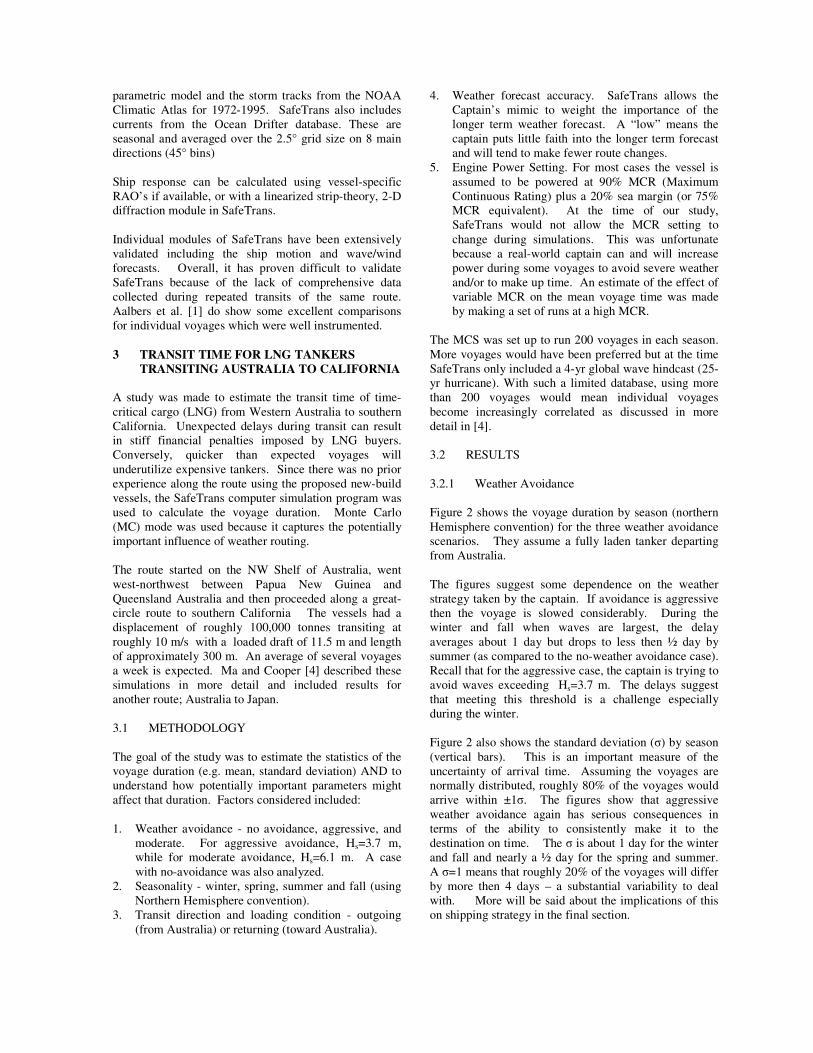
3.2 RESULTS
3.2.1 Weather Avoidance
Figure 2 shows the voyage duration by season (northern
Hemisphere convention) for the three weather avoidance
scenarios. They assume a fully laden tanker departing
from Australia.
The figures suggest some dependence on the weather
strategy taken by the captain. If avoidance is aggressive
then the voyage is slowed considerably. During the
winter and fall when waves are largest, the delay
averages about 1 day but drops to less then ½ day by
summer (as compared to the no-weather avoidance case).
Recall that for the aggressive case, the captain is trying to
avoid waves exceeding Hs=3.7 m. The delays suggest
that meeting this threshold is a challenge especially
during the winter.
Figure 2 also shows the standard deviation (σ) by season
(vertical bars). This is an important measure of the
uncertainty of arrival time. Assuming the voyages are
normally distributed, roughly 80% of the voyages would
arrive within ±1σ. The figures show that aggressive
weather avoidance again has serious consequences in
terms of the ability to consistently make it to the
destination on time. The σ is about 1 day for the winter
and fall and nearly a ½ day for the spring and summer.
A σ=1 means that roughly 20% of the voyages will differ
by more then 4 days – a substantial variability to deal
with. More will be said about the implications of this
on shipping strategy in the final section.

18
19
20
21
22
0.5
Vo
ya
ge
du
rati
on
(d
ay
s)
Aggressive
None
M oderate
Winter Spring Summer FallWinter Spring Fall
Figure 2: Mean voyage duration by season for three
weather avoidance scenario. Vertical bars show one
standard deviation.
3.2.2 Seasonality
This issue is already discussed to a large degree in
previous subsections. To summarize, the voyage
duration is clearly affected by the season for the
aggressive weather avoidance case. There is no seasonal
effect seen for the other two weather routing cases. The
seasonal dependence is clearly caused by storms in the
Northern Pacific during the Northern Hemisphere winter.
3.2.3 Transit direction
“Returning” simulations were made for the fall season
for the most likely weather routing scenario (moderate
weather avoidance, Hs=6.1m). The mean duration for the
returning trip is 17.3 days. This is 1.6 (8.4%) days faster
than the mean for the equivalent outbound voyage (18.9
days). There is also a significant drop in variability – the
return is roughly 1/3 of the outbound.
There are two obvious causes for changes in voyage
duration. First, the draft of the vessel is roughly 2 m less
for the return (9.5 m vs. 11.5 m). This means the hull
resistance will generally be less so the ship’s speed will
be higher under the same engine power settings. Second,
a close look at the SafeTrans database for currents
reveals that there is a favourable current on the return trip
which averages 25 cm/s over the route. Thus the relative
speed of the water past the ship is 25 cm/s less on the
return trip. Conversely, during the outbound trip, the
ship must oppose the current. If the mean speed of the
vessel is 9.4 m/s for the outbound (Fall, moderate
avoidance case), it is 9.9 m/s for the returning. This
results in a 5.4% difference in voyage duration between
outbound and return legs. That is slightly less than the
8.4% difference calculated by SafeTrans but well within
the range of uncertainty of the various assumptions made
including the wave added resistance and the contribution
from ship draft.
3.2.4 Weather forecast accuracy
SafeTrans allows the user to specify how much
credibility the captain should give to the longer-term
0
0.2
0.4
0.6
0.8
1
1.2
1.4
1.6
0.5 1.5 2.5 3.5
Long-term Forecast Confidence
Sta
nd
ard
De
via
tio
n (
da
ys
)
Moderate
Aggressive
High Medium Low
Figure 3: Variability of the voyage duration during
winter as a function of the captain’s confidence in the
longer-term weather forecast.
forecast. If the factor is “high” then the longer-term
forecast (> 5 day) is given relatively high impact on the
captain’s decisions. Conversely if the user specifies a
“low” factor, the captain is to take the longer term
forecast less seriously.
Figure 3 shows the impact of this parameter on duration
variability for winter. It shows no effect for the moderate
weather avoidance case – a result consistent with the lack
of importance of weather routing for this case.
More interestingly, the figure shows a sharp increase in
the variability of the voyage duration when the longer-
term forecast is heavily weighted. One possible
explanation for this is that the accuracy of weather
forecasts is known to become unreliable after 7 days in
regions where they have been well studied such as the
North Atlantic. It is likely that along the Australia-U.S.
route the forecast deteriorates more rapidly because of
the well known Pacific weather “data void”. Hence, by
weighting the longer-term forecast too heavily, the
captain is making moves based on statistically unreliable
data that results in wasted miles traveled.
3.2.5 Engine Power Setting (MCR)
Additional simulations were made using MCR settings of
80, 85, 90, and 95% for the fall season. It was found that
there was essentially no change in the variability of the
voyage duration or the MPM Hs. It was also found that
the mean travel time dependence on MCR can be
explained by a nearly linear relationship between MCR
and ship speed. From this it is concluded that the captain
can reduce his voyage time by as much as 5% by
increasing power. This is roughly double the variance on
travel time for the moderate and no weather avoidance
cases likely to be used. That means that the captain has
the power to overcome weather delays for virtually all
runs and still meet the mean travel time.

3.3 DISCUSSION
The results above show that there are significant
penalties if a low weather threshold (Hs ≤ 3.7 m) is used
in routing. If a more moderate threshold of 6.1 m is used
then weather routing does not change the voyage
duration appreciably compared to simply ignoring the
weather (no avoidance). We conclude that aggressive
weather avoidance would have significant negative
impacts with little obvious benefits for ships of the size
being considered. On the other hand, moderate weather
routing (Hs=6.1 m) has little substantial impact on
voyage duration and would almost certainly enhance
safety and fuel economy.
Another interesting finding is that the captain should not
give much weight to the long-term (> 5 day) weather
forecasts. It is conjectured that the forecasts are so
uncertain that a captain who considers them will simply
waste time with unnecessary avoidance.
Finally, the sensitivity studies suggest that the captain
will be able to meet the mean voyage duration for
virtually all runs by increasing engine power when facing
adverse weather.
4 TRANSIT TIME FOR CONTAINER SHIPS
TRAVELLING ACROSS THE N. ATLANTIC
SafeTrans MCS simulations were used to optimize the
voyage duration and economic risks of a westbound
trans-Atlantic crossing of container ships (Le Havre,
France to New York). The ship had a length of roughly
200 m, beam of 32 m, and mean travel speed of 11.5 m/s.
4.1 METHODOLOGY
Several scenarios regarding seamanship were examined:
• None. No re-routing or other changes.
• Limited. No re-routing but changes in ship heading
and speed.
• Full. Weather routing and seamanship.
The key factor when specifying weather routing is the
wave height above which the captain tries to re-route. In
this study, 4 thresholds for Hs were tested: 8, 7, 6, and 4
m. The resulting simulations were analysed to obtain
voyage duration (90% bandwidth), fuel consumption, 10-
voyage return maximum wave, and risk of damage
(economic risk).
4.2 RESULTS
The results of the simulations are summarized in Table 4.
Most of the columns are self-explanatory with the help of
the footnotes. The last column is a measure of the
damage risk. Damage is expected to occur if a given
acceleration level is exceeded, leading to sea-fastening
loads above Ultimate Limit State (ULS).
A number of trade-offs are readily implied by the Table.
For example as the Hs threshold goes down, the voyage
duration increases but the level of risk and most probable
maximum Hs goes down. The optimal scenario will
depend upon the owners risk aversion. The table also
shows that the Hs threshold is always exceeded. This is
primarily because of forecast uncertainty and/or
‘unavoidable’ bad weather. Another reason is that re-
routing involves human decision making processes and
these are obviously less than perfect [5].
Table 4: Summary of simulation results.
Sea-
manship Hs
1(m)
∆T 2(hrs)
Fuel
(t) Hs
3(m)
Risk 4(%)
None NA 149 (+45/-13) 570 9.3 0.94
Ltd NA 150 (+48/-14) 576 9.3 0.94
Full 4 188 (+110/-40) 675 6.9 0.63
Full 6 155 (+61/-20) 590 7.9 0.78
Full 7 151 (+45/-15) 574 8.3 0.83
Full 8 150 (+42/-14) 572 8.7 0.86 1Target threshold Hs. “NA” means “Not Applicable”; no weather
routing was used in this scenario. 2∆T is the voyage duration. Within this column, the 1st number
is the mean, the 2nd number is the increment added to the mean to reach
the 95% nonexceedence probability, and the 3rd number is the increment for the 5% probability. 3Most probable maximum Hs experienced during the 500 voyages. 4Damage criterion (ULS) assumed at 0.5 g vertical acceleration at bow
Figure 4 shows histograms of the sea states encountered
during the 500 voyages. From these one can conclude
that weather routing reduces the occurrence of the high
sea states by about a factor three.
Figure 4: Distribution of MPM Hmax for weather routed
(a) and non-routed voyages (b)
An example of the effect of weather routing during one
of the 500 simulated voyages is shown Figures 5 and 6.
The route actually sailed in 2004 is shown by the solid
thin line while the weather-routed, simulated voyage of
the same departure day is shown by the dashed line.
Figure 7 illustrates how SafeTrans can be used to
quantify the consequences of weather routing. If for
example the total economic risk is valued at 100m€, the
cost per ton HFO at 250€ and the cost of delay at 10k€
per hour, an optimum can be derived by calculating the
cost function:
Total merit = Risk*(100m€+FuelUse)*250€+delay*10k€

and plotting this cost function against decreasing weather
routing criteria settings as shown in Fig 7. The optimum
lies at lowest total merit; in this case with weather
routing criterion between 6 and 7 m Hs.
5 HEAVYLIFT OF A SUBMARINE
The SafeTrans MCS was used to assess the probability of
obtaining a suitable weather window within a specified
timeframe in order to undertake the heavy lift of a
Russian Nuclear Fuelled Submarine of about 3000T
displacement. The operation started with a 1-hour tow of
the submarine from the storage area to the loading site,
then a 3-hour operation to load the submarine onto the
Tranself which is 34,000T DWT, followed by a 12-hour
period to install seafasteners. Table 5 summarizes the
pre-determined thresholds for the operations. Figure 8
shows the submarine aboard the Tranself.
Figure 5: Actual historic route (solid) and weather
routed simulation (dashed).
.
Figure 6: Waves encountered on weather-routed (Hs=7
m, solid) and actual voyages (dashed line).
€0
€50,000
€100,000
€150,000
€200,000
€250,000
€300,000
€350,000
€400,000
€450,000
All Deci
sions
4m
All Deci
sions
6m
All Deci
sions
7m
All Deci
sions
8m
No R
e-ro
utin
g
No A
ctio
ns
DELAY COST
FUEL COST
ECONOMIC RISK
TOTAL MERIT
Figure 7: SafeTrans results can be used to optimize the
voyage by accounting for risk, fuel and delays.
5.1 METHODOLOGY
A start and completion date of 20 and 31 Aug 07 as per
the Charter Party and random years and days within the
timeframe were selected. A set of simulations totalling
40 and 400 voyages were utilised, the lower figure being
used initially to assess the feasibility of the task until the
full scale analysis could be performed. The location of
the offshore operation, the hull definition of the heavy-
lift vessel including its resistance curve, current and wind
forces and wind coefficients as well as the wind
coefficients of the cargo, roll and pitch motion, amount
of fuel and number of personnel onboard and the
allowable criteria for the operation below were selected.
The vessel response parameters that were analyzed were
the roll angle and pitch velocity of the centre of gravity
of the submarine.
Figure 8: Russian sub shortly after lift aboard the
Transhelf.
Table 5: Allowable criteria for the operation
Task Duration
(hrs)
Max Hs
(m)
Wind
(m/s)
Tow 1 0.6 10.3
Loading 3 0.4 8.7
Sea-
Fastening
12 1.0 12.9
5.2 RESULTS
The results indicated that there was a high probability of
experiencing a suitable weather window with the
necessary characteristics particularly when used in
conjunction with the daily and 5-day weather forecast for
the area. More specifically the results showed that:
• The pitching of the center of gravity of the vessel and
cargo could range from 0º to 7.5º, with those values
below 2º occurring within the suitable weather
window for the task.
• The number of occurrences where the maximum
wave-height was less than or equal to 1.2 m was met
our criteria. Additionally the probability of Hs less
than 1 m was 0.3 while that below 0.5 m was 0.7.

• Despite differing distributions of suitable conditions
within the 10 year period analyzed there was
indication that suitable conditions would occur at least
once within the specified timeframe in each year.
• Weather conditions were more likely to be favourable
within the first 4½ days of the allocated period.
The environmental conditions experienced during the
operation were at par with those predicted by the
SafeTrans computer programme. On this occasion the
actual operation was carried out successfully within the
allowable criteria in the first 4 days of the 10-day given
timeframe without effecting the charter of the heavy-lift
vessel. This demonstrates the usefulness of the program
to provide an enhanced assessment of the viability of the
operation; due to a better understanding of the
probability of suitable weather criteria occurring within a
specific timeframe; thereby enabling a more informed
decision to be made about reliance on the operational
outcome and the commitment of funds.
6 TRANSPORT OF A CRANE FROM S. KOREA
TO US EAST COAST
SafeTrans was used to study the transport of a crane
between South Korea and the U. S. East Coast during the
Northern Hemisphere winter. Figure 9 shows the vessel
loaded with the crane. The ship was 110 m long, had a
beam of 20 m and was capable of 7.5 m/s in calm seas.
Two routes were considered. Both went through the
Panama Canal. The shortest route is a more northern one
that travels along a great circle through the North Pacific
passing just south of the Aleutians (48ºN). The second
route takes a more sheltered southern route passing near
Hawaii and never going further north than the latitude of
Soul (35ºN).
6.1 METHODOLOGY
Three methods were used to analyze the loads at the
crane. SafeTrans provided two of those; one based on
VMC and the other based on the MCS with weather
routing. The third method is based on DnV [6] and uses
a wave factor for the North Atlantic portion of the
transport with an exposure period of 30 days.
Figure 9: Side view of heavy-lift ship with crane (cargo).
The results for the three methods and two routes are
summarized in Table 6. MCS mode is based on 250
voyages. Figure 10 defines the various forces and
motions used in the table. The “z” axis is aligned with
the vertical axis of the center of gravity (CoG) of the
crane. The blue plane represents the ship’s deck with
the y-axis is aligned along the ship’s beam. SafeTrans
results are based on the expected value for the 10-voyage
extreme.
In addition to accelerations, the forces at deck level are
calculated with SafeTrans. With the DnV approach, the
phasing between the acceleration components is not
known so conservative assumptions would have to be
made (not done in this paper) in order to calculate the
design deck loads.
6.2 RESULTS
Table 6 shows the SafeTrans estimates are always less
than the DnV estimates with the exception of pitch on the
northern route.
The largest difference is found for the cross-beam
accelerations which are nearly a factor of two different.
The two SafeTrans approaches are quite consistent; the
�
Figure 10: Definition of responses used in Table 6.
Table 6: Summary of results (units are mks).
Northern Southern
Signal DNV VMC MCS DNV VMC MCS
Hs NA 10.6 10 9.0 6.6
Roll 25.5 25 24 25.5 24.1 17.9
Pitch 10.2 12 11 10.2 9.2 9.2
Ax 6.2 3.8 3.1 6.2 3.2 3.1
Ay 5.9 5.2 4.7 5.9 4.9 3.6
Az 4.9 4.4 3.3 4.9 3.4 3.1
FxA 1170 865 920 856
FxB 1090 898 960 930
FyR 2780 2497 2600 1942
FzA 3260 2974 3060 2270
FzB 6600 5836 6050 4535
FzC 3350 3022 3130 2389

VMC results being slightly higher than MCS. This is
predictable given the effect of weather routing (missing
in VMC; present in MCS).
SafeTrans MCS provides considerable insight into the
tradeoffs involved in taking the northern and southern
routes. Figures 11 and 12 show the probability
distributions for voyage duration. The most probable
duration for the northern route is about 2 days shorter
than the southern route, and the northern route shows
considerably less variability. On the other hand, Table 6
shows the northern route exposes the crane to
considerably higher motions. Obviously, the final choice
for the route would depend on how close allowable loads
and motions are to the calculated values (accounting for
inherent safety factors) , and to the owner’s risk aversion.
7 BARGE TRANSPORT OF A SPAR FROM
DUBAI TO GULF OF MEXICO
SafeTrans was used to study the transport of a large
production spar from Dubai (UAE) to the Gulf of Mexico
routed via the Suez Canal starting in October. The spar
was mounted on a large heavy-lift barge which was
towed by a tug as depicted in Figure 13.
Figure 11: Histogram of voyage duration from
SafeTrans MCS for the southern route.
Figure 12: Histogram of voyage duration from
SafeTrans MCS for the northern route.
7.1 METHODOLOGY
Three methods were used to estimate the 10-yr Hs during
the voyage: SafeTrans MCS and VMC modes and the
traditional 10-yr Hs [6]. The ship transit speed was
determined from MCS and VMC. For the more
traditional approach, the speed must be specified so two
values were used.
Figure 13: Front Runner spar loaded on the Zhong Ren
3 being pulled by a tug.
7.2 RESULTS
Table 7 summarizes the results. The 10-yr return-period
Hs from the VMC analysis correlates well with the
conventional 10-yr criteria based on the slower speed
while the Hs from the MCS analysis is considerably
lower. MCS runs were based on 100 voyages. The latter
is consistent with MCS’s ability to incorporate weather
routing and safehavens. It is important to remember that
MCS provides encountered wave values, meaning they
are an average of the waves encountered within
simulated voyages. Given the above conclusion on MCS
statistics, one can understand that, for weather routed
transports and tows, the most probable maximum value is
not the design value.
Table 7: Comparison of traditional method and
SafeTrans.
Method Transit Spd
(m/s)
10-yr Hs (m)
Traditional 1 3.1 8.0
Traditional 2 3.3 7.0
MCS 3.6 5.7
VMC 3.4 8.0
7.3 DISCUSSION
Both SafeTrans MCS and VMC indicated a vessel speed
of roughly 3.5 m/s, about 10% higher than the design
team’s collective intuition had suggested. Initially, the
team had considered 3.5 m/s but dismissed it as too
optimistic. The team were concerned that a spar had
never been towed on a barge and believed 3.1 m/s would
be more appropriate. However, SafeTrans results
prompted a reassessment. Subsequently, SafeTrans was
used to investigate the risks involved using a restricted
tow with a design sea state of 7 m. Restrictions were

imposed by at three hold points along the route where a
shipboard evaluation of the current weather condition
and forecast was performed by the captain before
proceeding forward. Specifically, the hold points were:
1. Jebel Ali yard just prior to entering the Indian Ocean.
2. Suez Canal just prior to entering the Mediterranean.
3. Gibraltar just prior to entering the Atlantic.
SafeTrans MCS was used to study the consequences of
using a threshold of Hs of 7 m to make a go/no-go
decision at each hold point. During the 100’s of MCS
voyages, Hs never exceeded 7 m.
With the insight gained from this further analysis, the
tow proceeded with the above strategy. In October 2003,
the Front Runner spar left Dubai loaded on the barge. It
arrived in Mississippi, USA without incident on
December. Daily reports from the vessel showed that at
no point during the voyage was the cargo exposed to seas
greater than the 7 m threshold.
8 REPEATED VOYAGES OF CARGO SHIPS
FROM WESTERN EUROPE TO ICELAND
Over the span of 1.5 years, 12 voyages were made to
transport large equipment from western Europe to new
smelter on Iceland. Mean speed for the large cargo
vessels varied between 4.5-6 m/s depending on the
vessel and the time of year. This translated to a voyage
duration ranging from four days in the summer to over
six days in the winter. Figure 14 shows a photo of the
vessel loaded with some of the modules.
8.1 METHODOLOGY
Two voyages were considered both departing from
Wilhelmshaven, Germany. The first voyage involved the
transport of 6 modules in December and the second
voyage transported a large 660 tons vacuum ship
unloader during June. Six safehavens were specified in
SafeTrans along the route.
Figure 14: Picture of cargo vessel loaded with smelter
modules.
SafeTrans’ MCS (200 runs) was used to determine the
acceleration level at predetermined locations. For the
first voyage the center of gravities of the six modules
were added manually and for the second voyage the
center of gravity of the large unloader was selected. Both
voyages were carried out with the same ship type and
with weather avoidance thresholds set to Hs 7 m and
wind speed 15 m/s.
In addition to the SafeTrans calculations the maximum
accelerations at the same locations to be expected
according to DNV rules [6, Part 3, Chapter 1, Section 4]
for ships were calculated as well. These rules are based
on a North Atlantic voyage during wintertime that give
values for the maximum acceleration level at a selected
spot based on parameters of the ship and the loading
condition.
8.2 RESULTS
Table 8 shows the results. For the December voyage only
2 modules are included: module 1, which is the most
forward upper-deck module, and module 2, also an
upper-deck module stowed near the ship’s longitudinal
CoG. It was interesting to discover that the DNV results
for the transversal and vertical acceleration for all cargo
locations are exceeded during the December voyage. In
Table 8: Comparison of voyage results from SafeTrans
and DNV All units are mks unless otherwise stated.
DNV
WINTER SUMMER
Hs 5.0 5.0
Wind Spd 15 15
G'M (m) 1.20 1.40
Time frame Dec June
Distance, speed
duration (hrs) - 130 89
mean distance - 1618 1589
mean speed - 4.6 6.1
Accelerations (m/s2)
x COG Module 3.1 2.2
y COG Crane 1 3.8 4.2
z COG Crane 1 3.1 3.7
x COG Crane 2 3.1 2.2
y COG Crane 2 3.8 3.9
z COG Crane 2 2.2 3.1
x COG Vacuum Ship 3.5 1.9
y COG Vacuum Ship 4.6 1.9
z COG Vacuum Ship 2.2 2.0
Motions (m and º )
x COG ship - 7.0 3.5
y COG ship - 6.2 3.6
z COG ship - 7.5 3.2
roll COG ship - 15.8 7.7
pitch COG ship - 8.3 4.8
yaw COG ship - 6.7 4.1
SafeTrans

contrast, SafeTrans results for the summer voyage are
well below those of the DNV method. Also note the
difference in mean voyage duration between the summer
and winter voyage.
8.3 DISCUSSION
The results suggest that a more thorough evaluation of a
particular voyage using a tool like SafeTrans can yield
significant differences from a standard engineering
method. Furthermore it suggests that the DnV method
may yield unconservative results in some cases.
9 FPSO DESIGN OFF W. AFRICA
The SafeTrans MCS was used to estimate probability
distributions for various response parameters for a FPSO
(Floating Production Storage Offloading vessel) turret-
moored in deep water about 500 km south of Ghana,
West Africa. Figure 15 shows a front view of the FSO.
9.1 METHODOLOGY
The RAO's of the FPSO were specified and then the
MCS was run for 10 years with a departure day every
three days. The voyage route was essentially “no
movement”. Weather routing was turned off.
The peak responses from the simulated time series were
extracted from the SafeTrans runs and fit with a Weibull
distribution.
9.2 RESULTS
Figure 16 shows an example of the peaks of vessel pitch
fitted to a Weibull distribution. Table 9 shows the design
values at various return intervals which were extracted
from the Weibull plots.
9.3 DISCUSSION
Historically, most offshore facilities have been designed
with a two-step process. First, the metocean specialist
derived the n-yr wind , wave, etc. Then the response
Figure 15: Front view of FPSO
Weibull graph
0.00E+00
5.00E-01
1.00E+00
1.50E+00
2.00E+00
2.50E+00
3.00E+00
3.50E+00
4.00E+00
0.1 1 10 100
Signal Amplitude
Pro
ba
bil
ity
of
exc
ee
de
nc
e
[L
n(-
Ln
(pro
ba
bil
ity
))]
motion pitch COG [MCSid = 0-121]
Figure 16: Weibull for Pitch
The results of the simulations are presented in Table 9.
Table 9: Summary of simulation results
Return Period Heave
(m)
Pitch/Roll
(deg)
1 year 5.10 2.4
10 year 5.75 3.0
100 year 6.40 3.5
Expert made a single run with a response model to
determine the presumed n-yr motions and loads. Of
course, the preferred approach is to determine the n-yr
response directly, and this is what SafeTrans
conveniently provides. However, a word of caution is in
order – the uncertainty of the longer return periods such
as 100-yrs or greater may be quite large in some parts of
the world given that SafeTrans only includes a 10-yr
wind-wave database (24-yr hurricane).
10 SUMMARY AND CONCLUSIONS
This paper describes six case studies of SafeTrans
applications ranging from tug-barge and self-propelled
transports to the design of a stationary FPSO. These
applications also cover a wide range of routes, durations,
and transit speeds.
One of the unique capabilities of the SafeTrans MCS is
its ability to mimic the weather-routing that is now
routinely employed by the shipping industry. Results
from the case studies consistently show that including
weather-routing will reduce the expected cargo/vessel
motions (or it’s proxy, Hs) below those calculated using
methods that don’t consider weather routing. The degree
of reduction depends greatly on the route, time of year,
distance to safe havens, and transport speed. For
example in one of our case studies, the barge transport of
a spar, the reduction in the 10-yr Hs was roughly 20%.
The value of including weather routing in the analysis is
not limited to reductions in motions. One can also use
SafeTrans to investigate the effect of different weather
routing restrictions on the risk of achieving a successful
transport or voyage. At least four of the case studies
illustrate this benefit: the LNG, containership, barge-
spar, and submarine transports. In these four cases,
SafeTrans was used to find an Hs threshold for weather
routing that was easily met with no substantial adverse
impacts on the transport’s duration. In the other case
study, the transport of cranes, SafeTrans provided the
basic inputs that could be used in a further benefit-cost
analysis to optimize the route.
It should also be remembered that SafeTrans MCS
provides the ability to do fairly complicated frequency-
domain motion analysis using time series of
simultaneous Hs, Tp, wind speed, etc. Such analysis will
account for joint statistics of these parameters and will
almost certainly be more accurate than traditional
estimates using probabilities. The differences in
calculated motions can be substantial, e.g. in the case of
the transport of cranes, the expected value for the cross-
beam acceleration was a factor of two less than a
traditional analysis would suggest. SafeTrans also
provides an interesting new tool to do a thorough
response-based design of stationary floating facilities like
FPSO's.
Overall, these case studies illustrate the versatility of
SafeTrans and demonstrate its ability to develop less
conservative and more comprehensive criteria than
traditional methods.
11 REFERENCES
1. Aalbers, et al., ‘SafeTrans: A new software system
for safer rig moves’ Proc. Jackup Symposium, Imperial
College, 2001.
2. Aalbers, et al., ‘Voyage acceleration climate: a new
method to come to realistic design values for ship
motions based on the full motion climate for a particular
transport’, 5th
Jack-up Symposium, London, 1995
3. Aalbers, A. B. and C. E. J. Leenaars, ‘Two years of
acceleration measurements on Dock Express heavy-lift
vessels compared with predicted values for several
design methods’, RINA Spring Meeting, London, 1987.
4. Ma, W. and C. Cooper, ‘Estimating the Voyage
Duration of Transoceanic LNG transports’, Offshore
Marine & Arctic Engr. Conf., 67398, 2005.
5. Aalbers and Van Dongen, Weather routing:
uncertainties and the effect of decision support systems,
Paper 0041, MOSS conference Singapore, 2008
6. DNV Rules for Classification of Ships, Part 3, Chapter
1, Section 4, January, 2005
12 AUTHORS’ BIOGRAPHIES
Albert B. Aalbers is a Senior Researcher at the
Maritime Research Institute Netherlands (MARIN)
where he manages the Maritime Innovation Programme
and is responsible for co-ordination of R&D initiatives in
the maritime construction and offshore service industry.
Cortis Cooper is a Fellow at Chevron Energy
Technology Company where he is responsible for
developing metocean criteria for Chevron’s world-wide
operations.
Stephen Quinn, OBE, is Assistant Director Mooring,
Towing & Plans within the Salvage and Marine
Operations Integrated Project Team, U. K. Ministry of
Defence (MoD). He is responsible for all MoD heavy-
lift, coastal and ocean towing and all strategic fleet
moorings worldwide.
Cees Leenaars, is managing director of Leenaars Marine
and Offshore Design. His previous positions included
R&D manager at Dockwise and engineering operations
manager at Dock Express Shipping.
Sjaak Scholten, is a Naval Architect and has worked for
Jumbo Shipping since 2002 as a Project Engineer where
he is responsible for the technical preparation of heavy-
lift transports and installation projects.
James Vavasour is a Naval Architect who has worked
for MatthewsDaniel since 2002 as a Lead Project
Engineer where he is responsible for the technical and
procedural review of heavy-lift transports and major
offshore installation projects in the Gulf of Mexico
Kees Jan Vermeulen is a Naval Architect who works as
a Senior Project Engineer for Jumbo Shipping where he
is responsible for the technical preparation of heavy-lift
transports and technical feasibility analyses of offshore
projects.
Roel Verwey is Manager of the Engineering Department
at BigLift Shipping BV where he is responsible for the
development of engineering methods and for the
technical preparations of heavy lift transports.