Capital Punishment and Deterrence: Understanding Disparate Results

Steven N. Durlauf*

Chao Fu*

Salvador Navarro**

*University of Wisconsin at Madison **University of Western Ontario

12/15/11 Draft

Abstract The panel data literature on deterrence and capital punishment contains a wide range of empirical claims despite the use of common data sets for analysis. We interpret the diversity of findings in the literature in terms of differences in statistical model assumptions. Rather than attempt to determine a “best” model from which to draw empirical evidence on deterrence and the death penalty, this paper asks what conclusions about deterrence may be drawn given the presence of model uncertainty, i.e. uncertainty about which statistical assumptions are appropriate. We consider four sources of model uncertainty that capture some of the economically substantive differences that appear across studies. We explore which dimensions of these assumptions are important in generating disparate findings on capital punishment and deterrence from a standard county-level crime data set.

Corresponding Author: Durlauf, Department of Economics, University of Wisconsin, Madison WI 53706, sdurlauf@ssc.wisc.edu. We thank Timothy Conley and David Rivers for many helpful insights. Durlauf thanks the University of Wisconsin Graduate School and Vilas Trust for financial support. Hon Ho Kwok and Xiangrong Yu have provided outstanding research assistance.

1

1. Introduction

The effectiveness of capital punishment in deterring homicides, despite decades

of empirical work, remains very unclear. This is so despite the fact that the Supreme

Court’s moratorium on capital punishment and the subsequent adoption of capital

punishment by a subset of states, combined with very different rates of execution in those

polities with capital punishment, would seem to provide an ideal environment for

identifying the magnitude of deterrence effects using panel data methods. Focusing on

post-moratorium studies, one can find papers that argue that post-moratorium data reveal

large deterrent effects (Dezhbakhsh, Rubin and Shepherd (2003), Zimmerman (2004)),

fail to provide evidence of a deterrent effect (Donohue and Wolfers (2005), Durlauf,

Navarro, and Rivers (2010)), or that provide a mixture of positive deterrence negative

deterrence (brutalization) effects depending on the frequency of execution (Shepherd

(2005)).

The presence of disparate results on the deterrent effect of capital punishment is

not, by itself, surprising. Social scientists have long understood that the data “do not

speak for themselves” and so empirical analyses that involve substantive social science

questions such as the measurement of deterrence, can only do so conditional on the

choice of a statistical model. The disparate findings in the capital punishment literature

reflect this model dependence. This is even true when one conditions on the modern

panel literature in which the various models typically represent statistical instantiations of

Becker’s (1968) rational choice model of crime. Thus, a common basis for

understanding criminal behavior, in this case murder, is compatible with contradictory

empirical findings because of the nonuniqueness of the mapping of the underlying

behavioral theory to a statistical representation suitable for data analysis.

This paper is designed to understand the sources of the disparate literature

findings. Specifically, we consider how different substantive assumptions about the

homicide process affect deterrence effect estimates. From our vantage point, alternate

models of the homicide process are the result of different combinations of assumptions.

Since there is no a priori reason to assign probability 1 to any of the models that have

been studied in the literature or our own new models in this paper, our approach respects

2

and tries to constructively address the fact that the evaluation of the deterrent effect of

capital punishment constitutes a context in which one must account for the presence

model uncertainty.

The closest predecessor to this paper is Cohen-Cole, Durlauf, Fagan, and Nagin

(2009), which employed model averaging efforts to adjudicate the different findings of

Dezhbakhsh, Rubin and Shepherd (2003) and Donohue and Wolfers (2005). Cohen-

Cole, Durlauf, Fagan and Nagin were especially concerned to illustrate how model

averaging could address the problem of different papers coming to diametrically opposite

conclusions because of minor differences in model specification. As such, the purpose of

the exercise was, to a major extent, the integration of disparate deterrence estimates

across papers into a single number. Cohen-Cole et al were thus able to draw conclusions

about the disagreement between Dezhbakhsh, Rubin and Shepherd and Donohue and

Wolfers, finding that intermodel uncertainty was sufficiently great that no firm inferences

about deterrence were possible for the data set under study.

In contrast, the current paper takes a broader view of the capital punishment and

deterrence literature in attempting to understand why the literature has generated very

disparate results. We explore a broader set of modeling assumptions so that a more

general, and we think basic, set of sources of disagreements across papers are considered

when evaluating what the data reveal about capital punishment and deterrence. Further,

we consider models that have not previously appeared but, for theoretical reasons, in our

judgment should be part of the model space. Finally, unlike Cohen-Cole, Durlauf, Fagan

and Nagin, we are not primarily interested in reducing the model-specific estimates of

deterrence down to a single number. Instead, our goal is to understand which substantive

assumptions matter in determining the sign, magnitude and precision of various model-

specific deterrent effects.

We explore four sources of model uncertainty. Each, we believe, represents a

fundamental issue in modeling the homicide process from which deterrence estimates are

obtained. In all cases our object of interest, the deterrent effect, is measured as the

marginal number of lives saved by an additional execution. This is a purely statistical

definition. We are not concerned with efforts such as Shepherd (2005) to draw

conclusions about distinct behavioral mechanisms that distinguish brutalization effects

3

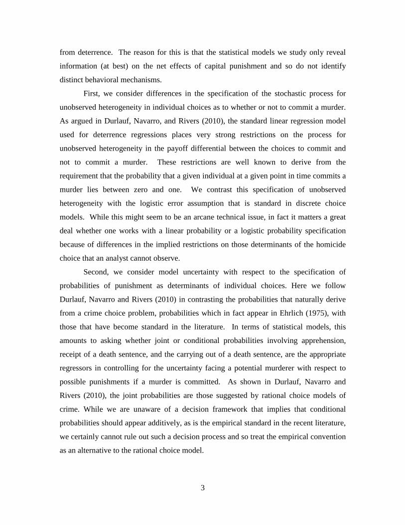
from deterrence. The reason for this is that the statistical models we study only reveal

information (at best) on the net effects of capital punishment and so do not identify

distinct behavioral mechanisms.

First, we consider differences in the specification of the stochastic process for

unobserved heterogeneity in individual choices as to whether or not to commit a murder.

As argued in Durlauf, Navarro, and Rivers (2010), the standard linear regression model

used for deterrence regressions places very strong restrictions on the process for

unobserved heterogeneity in the payoff differential between the choices to commit and

not to commit a murder. These restrictions are well known to derive from the

requirement that the probability that a given individual at a given point in time commits a

murder lies between zero and one. We contrast this specification of unobserved

heterogeneity with the logistic error assumption that is standard in discrete choice

models. While this might seem to be an arcane technical issue, in fact it matters a great

deal whether one works with a linear probability or a logistic probability specification

because of differences in the implied restrictions on those determinants of the homicide

choice that an analyst cannot observe.

Second, we consider model uncertainty with respect to the specification of

probabilities of punishment as determinants of individual choices. Here we follow

Durlauf, Navarro and Rivers (2010) in contrasting the probabilities that naturally derive

from a crime choice problem, probabilities which in fact appear in Ehrlich (1975), with

those that have become standard in the literature. In terms of statistical models, this

amounts to asking whether joint or conditional probabilities involving apprehension,

receipt of a death sentence, and the carrying out of a death sentence, are the appropriate

regressors in controlling for the uncertainty facing a potential murderer with respect to

possible punishments if a murder is committed. As shown in Durlauf, Navarro and

Rivers (2010), the joint probabilities are those suggested by rational choice models of

crime. While we are unaware of a decision framework that implies that conditional

probabilities should appear additively, as is the empirical standard in the recent literature,

we certainly cannot rule out such a decision process and so treat the empirical convention

as an alternative to the rational choice model.

4

Third, we consider model uncertainty from the vantage point of heterogeneity in

the deterrent effect of murders, contrasting the assumption in Shepherd (2005) that the

deterrent effect varies across states with the standard assumption in the literature that the

same parameters apply to all states. The model uncertainty we consider contrasts two

cases: one in which the deterrent effect is state-specific and one in which the deterrent

effect is constant across states. This form of model uncertainty addresses concerns that

have been raised that the skewed distribution of executions across US states renders the

interpretation of a single deterrent effect problematic. The most prominent example of

this concern is Berk (2005) which questions claims of a deterrence effect from interstate

data because of the concentration of executions in a few states, and their absence in many

state-year observation pairs. As stated, Berk’s criticism is not an obvious a priori

objection to the claims of the deterrence literature. For example, the success of a polio

vaccine based on trials in Texas would not be regarded as self-evidently meaning that the

vaccine’s efficacy in other states is uninformed by the Texas data. In other words, Berk’s

argument has import only if the concentration in a few states means that extrapolability

findings for death penalty states to other states is not warranted.1 Shepherd’s introduction

of state-specific execution effects is a constructive way to formalize the concern over

extrapolability and indeed does so in a fashion that is more general than what we interpret

as Berk’s criticism.2

Fourth, we address model uncertainty in the handling of cases in which a given

polity-time pair exhibits 0 murders. Once the murder rate is understood as a probability,

standard models have difficulty in predicting 0 murders.3 For the most part, the literature

(e.g. Dezhbakhsh, Rubin and Shepherd (2003), Mocan and Gittings (2003), Zimmerman

(2004), Donohue and Wolfers (2005)) has sidestepped this difficulty by using aggregate

1The treatment effect literature takes a much more sophisticated view of heterogeneity of effects of a given policy across individuals; see Abbring and Heckman (2007) for a review. 2Berk estimates a nonparametric regression relating number of executions to homicides. State-specific effects thus relax the assumption that two states with similar number of executions should exhibit the same deterrent effect. 3Note that this is a distinct concern from whether political unit-time pairs with zero homicides are or are not exchangeable with those that have non-zero homicides, which is subsumed in our third level of model uncertainty.

5

versions of the linear probability model that do not restrict predicted murder rates to live

in the [0,1] interval. By using linear regression models with the murder rate on the left

hand-side, the polity-time pairs with zero murders can simply be included as part of the

model. However, as shown in Durlauf, Navarro and Rivers (2010), once a properly

specified probability model is used as the basis to construct the estimating equation, the

left hand side variable (an appropriately transformed version of the murder rate) is no

longer defined for zero-murder observations. To deal with this problem, under an

assumption of selection on observables, Durlauf, Navarro and Rivers drop these zero-

murder observations from the analysis. In this paper we additionally consider what

happens when, in models based on the linear probability model, one confronts the zero-

murder observation by not including them in the analysis, even though mechanically they

could be included. More importantly, we generalize (for both linear and non-linear

probability models) the analysis to allow for selection on unobservables. To do so, we use

a control function approach to account for the possibility that polity-time observations

with zero murders differ from those with positive murders in ways that are unobservable

to the econometrician.

Section 2 of the paper outlines the way we think about model uncertainty. Section

3 discusses data. Section 4 describes the model space we employ to evaluate deterrence

effects to capital punishment. Section 5 provides empirical results on deterrence effects

across models. Following the literature, we place particular emphasis on net lives saved

per execution. Section 6 concludes.

2. Model uncertainty: basic ideas

In this section, we discuss the basic idea of model uncertainty. The intuitive idea

undoubtedly has been understood throughout the history of statistics, but the way we treat

the problem appears to trace back to Leamer (1978). Constructive approaches for

addressing model uncertainty have been an active area of research in the last 15 years

with particular interest in model averaging, which is a principled procedure for

combining information across models. Draper (1995) provides a still useful conceptual

6

discussion, Raftery, Madigan, and Hoeting (1997) is a seminal contribution on the

implementation of model averaging in linear models and Hoeting, Madigan, Raftery and

Volinsky (1999) and Doppelhofer (2008) are useful overviews. Our own approach is

similar in spirit to Leamer (1983) in that we are interested in exploring how different

assumptions affect deterrence estimates, although we do not endorse the extreme bounds

approach to assessing whether an empirical claim is robust or fragile with respect to a

given data set.

The basic idea of model uncertainty is simple to explain. Suppose one wants to

calculate a deterrence measure D. Conventional frequentist approaches to empirical work

produce estimates of this measure given available data d and the choice of a model m:

( )ˆ ,D d m (1)

Conventional analyses of deterrence estimates derive from the choice of m

in (1). Of course, authors are typically sensitive to issues of the robustness of deterrence

estimates and so typically vary m relative to some baseline. That said, it is also a fair

statement that this variation is typically local to the baseline and is implemented in an ad

hoc fashion, by which we mean the typical analysis considers whether a result is robust

relative to some baseline model by using intuition to suggest modifications of the

baseline. Similarly, critiques of the robustness of a particular paper’s claims often

proceed on ad hoc alternate specifications that were not originally considered.

The difficulties created by model uncertainty are well illustrated in the conflicting

claims of Dezhbakhsh, Rubin, and Shepherd (2003) and Donohue and Wolfers (2005).

Dezhbakhsh, Rubin, and Shepherd (2003) use county level data to conclude an additional

execution of a murderer saves a net 17 lives.4 Donohue and Wolfers (2005) critique

argues that the Dezhbakhsh, Rubin, and Shepherd deterrence estimates are fragile (i.e.

can be reversed) based on two different deviations from the baseline regression that

appeared in the original paper. Specifically, Donohue and Wolfers relax the assumptions

that 1) certain instrumental variable coefficients are constant across time and 2) 4By net, we mean that Dezhbakhsh, Rubin, and Shepherd find that each execution deters 18 murders.

7

comparability of the homicide data process for California and Texas with the rest of the

country; this amounts to dropping the two states from the sample. Dezhbakhsh and

Rubin (2011) respond by arguing most specifications of their model (out of a large set

whose construction is not justified per se) do find a deterrence effect.

This sequence of arguments is not constructive, because neither the fragility

finding nor the finding of deterrence effects in “most specifications” can be given a

formal statistical or decision-theoretic meaning. One way to proceed constructively is to

move beyond dueling specifications and ask what information is contained about

deterrence in a given model space. Cohen-Cole, Durlauf, Fagan, and Nagin (2009),

following Brock, Durlauf, and West (2003), employs the appropriate decision-theoretic

method for resolving the discrepancies between these two papers by using model

averaging, and find that the uncertainty surrounding the deterrence estimates swamps the

estimates themselves. At the same time, they find that the problem is not that

Dezhbakhsh, Rubin, and Shepherd use a model that fits the data less well than that of

Donohue and Wolfers; rather the problem is that neither model has any claim to be the

correct one, and each is best conceptualized as an element of a model space which

consists of different combinations of assumptions in the two papers. Relative to this

space, while the point estimate of lives saved is positive, intermodel uncertainty swamps

this value, in a fashion analogous to the standard error swamping the estimate of a

coefficient.

This paper is not interested in resolving the differences between a pair of papers,

as was the objective in Cohen-Cole, Durlauf, Fagan, and Nagin. Our objective is to

understand how different substantive assumptions about the homicide process affect

deterrence estimates. We do not make the assumption that the “true” homicide process is

part of the model space. While its absence would produce interpretation issues as to what

the deterrence estimates mean, it does not preclude an analyst from exploring the

sensitivity of deterrence estimates to alternative modeling assumptions.

Underlying our analysis is a particular concern for the use of deterrence studies as

a source of information for policymakers. In our judgment, the import of model

uncertainty for policy evaluation is that the prior comparison of models to select a best

model is inappropriate. A policymaker, in our view, is really only concerned about the

8

distribution of outcomes of interest, such as the murder rate, given a criminal sanction

regime for murderers. Knowledge of the true model has no intrinsic value but is only

useful to the extent that it informs the distribution of outcomes under alternative capital

punishment regimes. More formally, if the deterrent effect is going to be used in a policy

analysis, decision theory requires that model uncertainty be part of the overall description

of the uncertainty surrounding the effects of a given sanction regime, which exactly

parallels the argument Draper (1995) makes about properly describing the uncertainty

surrounding a forecast.

At the same time, we eschew an emphasis on model averaging as a mechanism

for reconciling different model-specific estimates. Our reason for this is that we focus on

what we regard as substantive differences between model specifications. Our goal is to

understand how these assumptions determine deterrence findings. Given our focus on

substantive differences, one can well imagine strong disagreements on the choice of a

prior by either analysts or policymakers. Put differently, we are less concerned with a

bottom line deterrence number than understanding how deterrence estimates vary across

the model space according to what substantive assumptions an analyst makes. We will

discuss posterior model probabilities under a uniform prior on the model space in order to

analyze the relative explanatory power that the different models have for the data we

employ. However, we are dealing with models where a priori reasons may justify one

model or set of models versus another, so that a given analyst might well choose to assign

a prior of 1 to a particular model or subset of the model space. Hence, these posteriors

are, in our judgment, useful as implicitly providing information on the Bayes factors

associated with the models.

3. Data

The data we use come from Dezhbakhsh, Rubin and Shepherd (2003). The data

set includes the murder rates for a panel of 3,054 counties for the 1977-1996 period. The

data on murders is obtained from the FBI Uniform Crime Reports (UCR). It also

includes data on county and state level covariates. In particular, we use data on the

9

county assault and robbery rates (also from UCR), NRA state level membership (from the

National Rifle Association), data on population distribution by age, gender and race as

well as population density (from the Bureau of the Census) and data on per-capita

income, income maintenance and unemployment insurance payments from the Regional

Economic Information System.

We also use county level data on murder arrests (UCR) and murder sentencing as

well as state level data on executions of death-penalty inmates (Bureau of Justice

Statistics) to estimate the probabilities of arrest, sentencing and execution. We follow

Dezhbakhsh, Rubin and Shepherd and estimate these probabilities as follows. The

probability of arrest is formed as the ratio of murders at time t . In order to account for

the lag between sentencing and arrest, the probability of sentencing conditional on arrest

is formed as the ratio of death sentences at t over arrest for murder at 2t − ; this lag is

meant to capture the average gap between a murder and an arrest, when an arrest occurs.

Since the average lag between sentencing and execution is six years, the execution

probability is constructed as ratio of executions at t to sentences at 6t − .5

Finally, the dataset also includes data on expenditures on police and judicial legal

system, prison admissions, (Bureau of Justice Statistics) as well as percentage of the state

population who vote Republican in presidential elections (Bureau of the Census). These

variables represent exclusion restrictions with respect to the murder equation, i.e. they are

variables that help predict the probability of punishment but that are not included in the

equation relating murders to these probabilities. As such, these variables may be used to

instrument for the endogenous probabilities of arrest, sentencing and execution.

4. Model space

Each element of our model space consists of an outcome equation for murder

rates in which the deterrent effect of capital punishment may be calculated from the

5Sometimes these probabilities are not defined since the denominator can be zero. To avoid losing observations, we impute values from lagged values of the probability (up to 4 periods) when possible.

10

presence of variables which measure probabilities associated with a murderer receiving

capital punishment. Other forms of heterogeneity are also included. Each of the models

we consider can be interpreted as a modification of the baseline regression in

Dezhbakhsh, Rubin, and Shepherd (2003), which is

( ) ( ) ( ), , , , , , ,c t c t A c t S c t E c t cc ttM P A P S A P E S Xβ β β θ θγ ξ= + + + + + + (2)

where ,c tM is a measure of the murder rate in county c at time t , ( ),c tP A is the

probability that a murderer is caught, i.e. the apprehension rate for murders. ( ),c tP S A is

the probability that an apprehended murderer is sentenced to death. ( ), c tP E S is the

probability that a death sentence is carried out given a death sentence. ,c tX are

demographic and economic characteristics of the county. cθ and tθ are county and time

fixed effects. ,c tξ is a zero mean residual that is assumed to be independent of ,c tX but

not of ( ), ,c tP A ( ), ,c tP S A and ( ), c tP E S .

We construct a model space by considering four distinct sources of model

uncertainty. It is appropriate to think of our analysis as forming models by the resolution

of the model uncertainty from each of these sources.

The first source of model uncertainty we consider is generated by alternative

assumptions on the underlying probability model generating equation (2). As will be

apparent, it is appropriate to consider this as model uncertainty about the distribution of

unobserved heterogeneity. This follows from considering how eq. (2) may be justified as

the aggregation of individual decisions in a population. In order to justify the linear

structure in (2) as the aggregation of individual choices in county c at time t , it is

necessary that the binary choices of the individuals obey a linear probability model; this

is shown in Durlauf, Navarro, and Rivers (2010).

Linear probability models are well known to impose very stringent assumptions

on the individual-level analogs of ,c tξ in order to ensure that probabilities are always

bounded between 0 and 1. For this reason, they are really only used for estimation

11

convenience. Further, standard assumptions on errors, such as normality or the negative

exponential distribution, imply a complicated relationship between individual level

variables, their associated distributions across the population, and aggregate behavior

rates. This is problematic when one is considering something such as the deterrent effect

of capital punishment, since the linearity in (2) will not hold for alternative unobserved

heterogeneity assumptions. For these reasons, we contrast (2) with a model in which the

individual murder choices obey the standard logit model. The logit functional form for

individual choices has the advantage that it also allows for a simple representation of the

aggregate murder rate in county c at time t . Durlauf, Navarro, and Rivers, show that

these aggregate murder rates will follow

( ) ( ) ( ),, , , , ,

,

ln1

c tc t A c t S c t E c t c t

c tc t

MP A P S A P E S X

Mβ β β θ θγ ξ

= + + + + + + −

. (3)

Notice that this form of model uncertainty involves the appropriate dependent variable in

the statistical model, and so is fundamentally different from the standard model

uncertainty question of the choice of variables in a linear regression.

Our second source of model uncertainty involves the choice of probabilities

employed in eqs. (2) and (3). We refer to this as model uncertainty about the

determinants of choice under uncertainty. The conditional probabilities that appear in eq.

(2) represent an assumption about how the capital punishment regime (by which we mean

the likelihood of various punishment outcomes) affects individual choices. This

specification appears in two of the most prominent studies in the panel literature on

capital punishment. What is surprising is that these are not the appropriate probabilities

to employ if potential murders obey the rational choice model of crime.6 Durlauf,

Navarro, and Rivers (2010) show that,7 under the linear probability model assumption,

6We are not sure why the probabilities that are implied by Bayesian decision theory, which were certainly understood by Ehrlich, see Ehrlich (1975) for example, are no longer the standard ones used in the death penalty and deterrence literature. 7To see why the probabilities in (2) are incorrect, as opposed to those that appear in (3), following Durlauf, Navarro, and Rivers (2010), let NA denote not apprehended, NS denote not sentenced to death, and NE denote not executed. Denote ( ),i tu ⋅ as the utility

12

the probabilities that derive from utility maximization produce the aggregate murder

equation

( ) ( ) ( ), , , , , ,, , ,c t c t A c t S c t E c t c tc tM P A P A S P A S E X γβ β β θ θ ξ= + + + + + + . (4)

The differences between (4) and (2) are immediate when one notes that

( ) ( ) ( ), , ,,c t c t c tP A S P S A P A= and ( ) ( ) ( ) ( ), , , ,, ,c t c t c t c tP A S E P E S P S A P A= ,8 so that the

probabilities in (2) interact to produce the regressors in (4). While we are unaware of any

formal justification for the use of conditional probabilities as appears in (2), we note that

there may be a justification for them on bounded rationality grounds. By this we mean

that the conditional probabilities are simpler than at least one of the joint probabilities.

While we do not go so far as to claim that the conditional probabilities are a natural way

to incorporate the presence of capital punishment on individual choices, we nevertheless

include such specifications in our model space.

Our third source of model uncertainty, following Shepherd (2005), allows for

state-specific coefficients in the probability of execution. We call this model uncertainty

of a murder by individual i at t under different punishment scenarios. Expected utility from a murder will equal

( )( ) ( ) ( ) ( ) ( ) ( )( ) ( )

, , , , , ,

, ,

1 Pr Pr , , Pr , , , ,

Pr , , , , .c t i t c t i t c t i t

c t i t

A u NA A NS u A NS A S NE u A S NE

A S E u A S E

− + + +

If the utility differences across punishment scenarios are constant, so that

( ) ( )( ) ( )( ) ( )

, ,

, ,

, ,

,

, , ,

, , , , .

A i t i t

S i t i t

E i t i t

u A NS u NA

u A S NE u A NS

u A S E u A S NE

β

β

β

= −

= −

= −

Then the form (4) is generated when decisions are aggregated under the linear probability model that produced (2). 8Note that in this derivation, we have made the substitution ( ) ( ), , ,c t c tP E S P E A S= , which follows from the fact that one has to be apprehended in order to be sentenced to death.

13

about state level heterogeneity. Formally, if one defines an indicator variable ,s cδ which

equals 1 if county c is in state s and 0 otherwise, Shepherd replaces ( ),c t EP E S β with

( ), ,, cs Ec t ss

P E Sδ β∑ in equation (2). Shepherd does not motivate her decision to

introduce state-level heterogeneity for this conditional probability while leaving the

coefficients on the other probabilities, and for that matter the other state level controls,

constant. However, while this suggests a broader conception of model uncertainty with

respect to state-level heterogeneity, we restrict ourselves to the type of heterogeneity

considered by Shepherd in order to maintain closer touch to the existing literature.

Our final source of model uncertainty arises as a consequence of the murder rate

being zero in many county-time observations in our data. Consider first the models based

on the logistic probability model. Since the left-hand-side variable is a log transformation

of the murder rate, this variable is not defined for those county-time pairs for which the

murder rate is zero. One possibility is to follow Durlauf, Navarro, and Rivers (2010) and

simply run the models dropping those observations for which the murder rate is zero.

This is a valid approach if the county-time pairs with zero murder rates are a random

subsample of the data given the observable characteristics we condition on. However,

there is no good reason to think that the zero-murder-rate observations are random. We

therefore introduce a fourth form of model uncertainty: model uncertainty about

exchangeability of county-time pairs with no murders and those with murders. While we

refer to this as uncertainty about exchangeability between subsets of observations, note

that it also encompasses issues normally associated with selection on unobservables.

In order to account for the potential endogeneity of the zero murder county-time

pairs, we employ control functions.9 In order to understand why the zero-murder-rate

observations may introduce selection bias, and to explain how the control function

approach solves the problem, consider a simplified version of equation (2)

, , ,c t c t c tM W ω ξ= + , (5)

9See Heckman and Vytlacil (2007) and Navarro (2008) for discussions of the control function approach.

14

where ,c tW represents all the covariates on the right hand side of (2) and ω represents

their associated parameters. For ease of exposition, we assume that ,c tW is independent

of ,c tξ , even though in our empirical analysis we allow for ( ), ,c tP A ( ), ,c tP S A and

( ), c tP E S (when we follow eq. (2)) or ( ),c tP A ( ), ,c tP A S and ( ), , ,c tP A S E (when we

follow eq. (4)) to be correlated with ,c tξ .

Define an indicator variable ,c tD that equals 1 if the murder rate in county c at

time t is positive and equals 0 otherwise. Following the logic originally developed in

Heckman (1979) this indicator variable is assumed to obey a “selection” equation, i.e. a

binary choice model for whether ,c tD is one or not, of the form

( ), , ,1 0c t c t c tD Y λ η+= > , (6)

where ,c tY may contain all the variables in ,c tW , but it may also contain other variables

that affect the selection equation but not the outcome. For expositional simplicity we

assume that ,c tY is independent of ,c tη , even though in practice we allow for correlation

between ( ) ( ) ( ), , ,, ,c t c t c tP A P S A P E S and ,c tη . Let

( ), , ,Pr 1|c t c t c tD Yπ = = (7)

denote the probability of having a positive murder rate conditional on ,c tY .

Consider estimation of the model of equation (5), conditional on the murder rate

being positive under the assumption that, given the observable characteristics one

conditions on, the subset of county-year pairs with positive murder rates is nonrandom,

i.e. that there is selection on unobservables into the positive murder rate case. Under

nonrandom selection,

15

( ) ( ), , , , ,,,| , 1 | , 1c t c t c t cc tt c t c tE M Y D W E Y Dω ξ= = + = . (8)

The second term in the right hand side of (8) is the selection bias that arises because we

can no longer assume that the observable characteristics are sufficient to ensure

orthogonality of regressors and model errors. The control function approach exploits the

fact that one can formulate ( ), ,, | , 1c t cc t tE Y Dξ = as a function of ,c tπ ,

( ), , , ,c t c t c t c tM W gω π ζ= + + (9)

such that, for a function ( ),c tg π (the control function), the new residual has conditional

zero mean (i.e. ( ), ,, | , 1 0c t c tc tE Y Dζ = = ).10 Furthermore, it follows that selection on

unobservables is a problem only when ,c tM depends on the function ( ),c tg π , a testable

restriction.11

Together, these four sources of uncertainty generate 20 distinct models. Figure 1

illustrates our four sources of model uncertainty and illustrates how the model space may

be described using a tree structure. The tree illustrates how the sources of model

uncertainty produce a sequence of models. The tree structure should not be interpreted as

producing a “hierarchy” for model uncertainty since it could have been constructed using

any order for the layers of model uncertainty.

5. Results

10To understand why this is the case, notice that , , ,1c t c t c tD Yη λ= ⇔ > −

( ) ( ), ,c t c tF F Yη ηη λ⇔ > − ( ), ,1c t c tFη η π⇔ > − , where Fη denotes the distribution function

of ,c tη . It then follows that we can write

( ) ( )( ) ( ), , , , , , ,| , 1 | 1 .c t c t c t c t c t c t c tE Y D E F gηξ ξ η π π= = > − ≡ 11See Heckman, Schmierer and Urzua (2010).

16

The exact specification for the baseline model we estimate is given by

, ,

, ,

, , , ,1 2 3

, , , 2 , 6

, , , ,1 2

, , , ,

/100000c s t

c s t

c s t s t s t

c s t s t s t

c s t c s t

c s t c s t

MurdersPopulation

HomicideArrests DeathSentences ExecutionsMurders Arrests DeathSentencesAssaults Robberies

Population Population

β β β

γ γ

− −

=

+ + +

+ + 3 , ,

,4 , , 5

,

, , .

c s t

s tc s t

s t

c t c s tc t

CountyDemographics

NRAmembersCountyEconomy

Population

CountyEffects TimeEffects

γ

γ γ

η

+

+ +

+ +∑ ∑

(10)

The remaining elements of the model space are variations of this baseline model

following the description in section 4.

Estimation follows a (adapted) two stage least squares algorithm. In the first stage

we regress the three endogenous probabilities in (10) (i.e. the first three terms on the right

hand side) against the exogenous covariates including the instruments described in the

last paragraph of Section 3. For the models where we have state-specific coefficients, we

do not possess a sufficient number of instruments for all of the state-specific probabilities

of execution. We solve this problem by interacting state dummies with the instruments in

order to create state-specific instruments (strengthening the assumptions accordingly).

In models where we correct for selection we introduce an intermediate step. We

first predict the probability of having a positive murder rate, ,c tπ , against the same

covariates in equation (10) plus the county population, making sure we instrument for the

potentially endogenous probabilities of arrest, sentencing and execution.12

In the second stage of the algorithm, we run equation (10) against the predicted

probabilities obtained in the first stage. When appropriate, we approximate the control

function in eq. (9) with the inverse-Mills ratio that arises from assuming joint normality

12When we instrument for the potentially endogenous probabilities of arrest, sentencing and execution in the selection model, the empirical results are virtually identical to the results we present, in which we assume these probabilities are exogenous.

17

of the residuals, i.e. ( ) ( )( )

,,

,1c t

c tc t

YY

gλφ

πλ

−=

−Φ − where φ and Φ are the density and

distribution functions of a standard normal random variable.13 In all models that include

a control for selection, we cannot reject the hypothesis that selection on unobservables is

present.

In evaluating deterrence effects, the literature emphasizes the number of net lives

saved per execution. For any model for the murder rate ( )M e , where e is the number of

executions, net lives saved is calculated as

( ) * 1M e

Net Lives Saved Populatione

∂= − −

∂ (11)

where ( )M ee

∂∂

is the derivative of the murder rate with respect to the number of

executions implied by each model.

Since the number of net lives saved varies by county, there is no unique way of

summarizing this metric. For all models, we present three different summary measures of

net lived saved. In the first case, we calculate net lives saved by evaluating the formula in

(11) at the average values for states having the death penalty in 1996 as in Dezhbakhsh,

Rubin and Shepherd (2003). For the other measures we present, for each of the 38 states

having the death penalty in 1996, we average (11) over counties. We then report either

the average over states or the median over states. Table 1 presents our estimated

measures of net lives saved. The model numbering in the table follows Figure 1. In all

cases, the confidence intervals are such that we cannot reject the hypothesis of zero

deterrence effects. Our confidence intervals are wider than those in Dezhbakhsh, Rubin,

13We also experimented using a semiparametric control function by plugging a fourth order polynomial in ,c tπ for ( ),c tg π . The results do not change qualitatively and are quantitatively very similar. The advantage of the normality assumption is that it allows us to more easily define the likelihood required for the calculation of posterior probabilities for model averaging.

18

and Shepherd (2003) because we follow Donohue and Wolfers (2005) and obtain

standard errors using the nonparametric bootstrap, clustering at the state level.14

Figures 2-4 provide a visual summary of how model assumptions determine

estimates of the net lives saved per execution, a statistic which has commonly been

treated as the “bottom line” of deterrence studies. Figure 2 presents the summary measure

of net lives saved when evaluation is made using the average characteristics of a 1996

death penalty state. Figures 3 and 4 present summary measures when one averages over

states (Figure 3) and when one takes the median effect over states (Figure 4). As shown

by the figures, regardless of which summary measure is used, the clustering of effects by

type of model used is striking. It clearly illustrates how different model assumptions

determine deterrence effect estimates. In general, we have the following major findings.

First, the estimates exhibit great dispersion across models. Depending on the

model, one can claim that an additional criminal executed induces 63 additional murders

or that it saves 21 lives if one evaluates at the X’s of the average death penalty state in

1996; that it induces 98 additional murders or saves 31 lives if one averages across 1996

death penalty states; or that it induces 22 more murders or saves 19 lives if one takes the

median net lives saved across 1996 death penalty states. This demonstrates the ease with

which a researcher can, through choice of modeling assumptions, produce evidence either

that each execution costs many lives or saves many lives. As such, we show that the

Donohue and Wolfers (2005) finding that the Dezhbakhsh, Rubin, and Shepherd (2003)

14For all models, the standard errors are sufficiently large that evidence of a deterrence effect is weak regardless of which model is employed. This suggests that the disagreement between Dezhbakhsh, Rubin, and Shepherd (2003) and Donohue and Wolfers (2005) on standard error calculations (in which we think that Donohue and Wolfers is preferable to Dezhbakhsh, Rubin, and Shepherd) is a first order issue. We do not emphasize this for two reasons. First, the paper is designed to understand how deterrence estimates are affected by modeling assumptions, not to assess statistical significance per se. Second, neither standard error approach is necessarily appealing because neither fully addresses potential cross-county dependence. We therefore do not regard either approach as spanning the set of plausible dependence structures for the county-level homicide regression errors. In other words, there is a distinct question concerning model uncertainty with respect to the probability structure of the unobserved heterogeneity in the county homicide processes which we do not explore. This type of model uncertainty does not affect the point estimates of the regressions under study and so functions independently from the model uncertainty we examine.

19

is driven by their particular choice of model is broader problem than the fact that the two

papers find different deterrent effects. We move beyond Donohue and Wolfers by

identifying how substantive modeling assumptions (as opposed to what can reasonably be

regarded as ad hoc variations of the Dezhbakhsh, Rubin, and Shepherd model) matter.

Put differently, we consider alternative modeling assumptions that help characterize the

literature, rather than identify a special set of assumptions that reverse the Dezhbakhsh,

Rubin, and Shepherd regression.

Second, a particular subset of models − linear models with constant coefficients −

always predict positive net lives saved (i.e. a deterrence effect). This subset contains all

cases in which a marginal execution saves lives. All other models predict negative net

lives saved for an additional execution under any of the three summary measures we use.

Our evidence is consistent with Shepherd (2005) who finds evidence of “brutalization”,

i.e. negative net lives saved, for some states when the effect is allowed to differ by state.

As opposed to Shepherd, we find that the summary effect is negative for models that

allow the effect to vary by state regardless of how one summarizes the different effects

across 1996 death penalty states.15 The assumptions of linearity and constant coefficients

thus are critical in the determination of the deterrence effect sign.

Third, the magnitudes of the point estimates of net lives saved, given a stance on

whether the deterrent effect is constant across states or not, differ mainly because of the

choice of linear versus logistic specifications. Controlling for the other three sources of

model uncertainty, the magnitudes of the point estimates from the linear models are

almost always larger (in absolute value) than those from the corresponding logistic

models.

How might information be aggregated across the model space to draw overall

conclusions on deterrence? Because one of the sources of uncertainty we consider

involves different sample sizes (i.e. sometimes dropping the county-time pairs with zero

murder rate), standard model averaging techniques cannot be employed. Instead, we

15One of the reasons our results for the linear model vary with respect to Shepherd, is that we do not restrict our averaging to states that have a statistically significant effect. We see no reason why such a restriction is justifiable, as the statistical significance of the summary transformation can be evaluated independently of the significance of the individual effects.

20

separate our model space into two subspaces, one containing all 8 models that drop the

county-time pairs with zero murder rate, and another containing the 12 models that

include all observations. For each subspace we calculate the posterior probability that m

is the correct model given the data d . That is, we calculate:

( ) ( ) ( )Pr Pr Prm d d m m∝ . (12)

It is immediate that the posterior probabilities reflect both the evidentiary support for

each model, as reflected in ( )Pr d m , as well as the researcher’s prior beliefs about the

models, ( )Pr m . Hence the data and the substantive a priori theoretical commitments

matter in determining the weights assigned to each model. Since we have no prior reason

to prefer one model over another, we employ uniform priors in the calculation of (12).

Finally, following Raftery (1995) and Eicher, Lenkoski and Raftery (2009) we

approximate ( )Pr d m using the Bayesian information criterion so that

( )( ) ( )( ) 11ˆPr ln Pr ,2

ln ln( ) ( ),m Nd m d O Nm k −+= −θ (13)

where N is the sample size, ( )ˆPr ,d m θ is the likelihood of model m evaluated at the

estimated parameter vector θ̂ and mk is the number of variables in the model.

Table 1 also reports the posterior probability of each model for the two model

subsets under our uniform model space prior assumption. Only two out of our twenty

models have positive posteriors. In each of our two model subspaces the logistic model,

with joint probabilities employed to measure deterrent effects, and with constant

coefficients, possesses a posterior probability of one (where in one case we drop the

county-time pairs with zero murder rate and in the other we control for selection on

unobservables). This is of interest since the joint probability specification is the one

suggested by the appropriate decision problem facing a potential murderer, and because

the logistic specification has more appealing statistical properties than the linear

21

probability model. We further note that the failure of the state-specific coefficients

models to receive any posterior weight suggests that the degrees of freedom lost in

allowing for additional coefficients is not compensated for by a superior goodness of fit.

In this sense, Shepherd’s generalization does not seem to be justified by the properties of

the data, if one works with a uniform prior, as is conventional in the model averaging

literature. Put differently, one needs a strong prior belief in state-specific coefficients in

order to place much weight on models that embody this feature.

For both of our model subspaces, the estimates suggest that an additional

execution leads to approximately 15 more murders being committed when evaluated at

the average characteristics of a 1996 death penalty state or when averaging across states.

When taking the median over states, the effect is about 13 additional murders when we

do not control for selection and about 6 additional murders when we do control for

selection. Hence, if one were to attempt to draw a conclusion from our model space,

based on averaging, this conclusion would be that the marginal effect of an execution on

the number of murders is positive. However, the standard errors of the estimates are of

the same order of magnitude as the estimates themselves, so this evidence is quite

weak.16

6. Conclusions

In this paper, we have examined how four different types of model uncertainty

affect deterrent effect estimates of capital punishment. We do this by considering

modifications of a panel regression model of Dezhbakhsh, Rubin, and Shepherd (2003),

which has been criticized for fragility by Donohue and Wolfers (2005). Our approach

16In the criminology literature, the possibility that executions can increase homicides is known as a brutalization effect. Cochran, Chamblin, and Seth (1994) argue that capital punishment can legitimize the taking of life in potential murderers’ minds. We note that one can produce an increase in murders from capital punishment based on rational choice deterrent arguments; for example, a murderer may have an increased incentive to kill witnesses if he already is facing the maximum penalty. Our point is that a positive relationship should not be regarded as perverse from the perspective of the economic model of crime, once one considers how deterrence affects decisions at the margin.

22

tries to move beyond debates about whose model specification is best by examining how

substantive modeling assumptions do or do not matter in deterrence effect estimates.

Our analysis finds that the choice of constant versus state specific coefficients

plays a key role in determining whether deterrence effects are positive or negative (i.e. a

brutalization effect is present). We further find that the magnitudes of the coefficients are

sensitive to whether a logistic or linear probability model is assumed for unobserved

heterogeneity. In contrast, neither the use of the theoretically appropriate joint

probabilities for capital punishment versus the conditional probabilities that have become

standard in the literature, nor the restriction of the analysis to county-time pairs with

positive numbers of murders have a first order effect on deterrence estimates. While we

see good theoretical reasons for preferring the use of joint rather than conditional

probabilities as regressors, and for using the selection correction when county-time pairs

with nonzero murders occur, for this particular exercise, neither of these theoretically

preferred assumptions appears to have a first order effect on estimates of net lives saved

for our model space.

Thus we conclude that an analyst’s assumptions on whether the marginal effect of

an execution on homicides is or is not state specific and whether or not one uses a linear

or logistic probability specification are the key substantive assumptions in determining

the magnitude of deterrent effects, at least as measured by the summary statistic of net

lives saved. Interestingly, these assumptions both involve the way that an analyst

addresses heterogeneity: in one case unobserved heterogeneity in parameters across

political units, and in the other the distribution of unobserved heterogeneity in the

determinants of homicides in these same units. Thus the disparity of deterrence claims

in modern capital punishment literature reflects one of the fundamental messages of

modern microeconometrics: the modeling assumptions made on unobserved

heterogeneity can control the findings of an empirical exercise. In this case, the (in our

judgment) relatively theoretically unappealing assumptions of constant state coefficients

and a linear probability model for unobserved heterogeneity are both needed to produce

estimates that an additional execution will save lives. Whether one agrees with our

assessment on what assumptions are better motivated by economic theory or not, our

results reinforce the message of Heckman (2000,2005): that questions such as deterrence

23

effects cannot be understood outside the prism of models and it is illusory to think that

questions such as the deterrent effect of capital punishment can be answered without

careful consideration of what assumptions an analyst is willing to make. The need for

judgment cannot be escaped in empirical work.

24

Logistic Model

Linear Model

Zeros

Zeros

Drop Zeros

Zeros

Zeros

Drop Zeros

Drop Zeros

Drop Zeros

Selection

Selection

Selection

Selection

Selection

Zeros

Drop Zeros

Selection

Drop Zeros

Zeros

By State

By State

By State

Fixed

Fixed

Fixed

Joint Probabilities

Conditional Probabilities

Joint Probabilities

Conditional Probabilities

By State

Fixed

Drop Zeros

Zeros

Drop Zeros

Selection

Selection L.C.F.D. (5)

L.C.F.S. (17)

L.C.F.Z. (1)

L.C.S.D. (6)

L.C.S.S. (18)

L.C.S.Z. (2)

L.J.F.D. (7)

L.J.F.S. (19)

L.J.F.Z. (3)

L.J.S.D. (8) L.J.S.S. (20)

L.J.S.Z. (4)

G.C.F.D. (9)

G.C.F.S. (13)

-

G.C.S.D. (10)

G.C.S.S. (14)

-

G.J.F.D. (11)

G.J.F.S. (15)

-

G.J.S.D. (12)

G.J.S.S. (16)

-

Zeros

Figure 1: Model Space

25

Table 1

Not Selection Corrected

Linear Linear Linear Linear Linear Linear Linear Linear Logistic Logistic Logistic Logistic

(1) (2) (3) (4) (5) (6) (7) (8) (9) (10) (11) (12)

Net Lives Saved at Avg. X

18.45 -51.71 16.60 -41.33 16.51 -63.57 14.98 -45.04 -1.73 -16.54 -2.71 -14.55

(Std. Error) (43.53) (45.65) (44.73) (32.73) (45.74) (49.75) (48.16) (35.23) (20.87) (26.18) (22.14) (12.34)

Mean Net Lives Saved

22.44 -86.28 26.04 -37.24 20.10 -98.52 23.55 -40.31 -2.22 -42.83 -4.96 -15.17

(Std. Error) (50.06) (37.31) (67.51) (23.71) (52.57) (41.37) (72.07) (25.19) (33.71) (34.93) (45.15) (17.53)

Median Net Lives Saved

17.12 -17.93 15.60 -9.36 15.31 -22.04 14.07 -8.75 -1.93 -7.00 -3.59 -13.45

(Std. Error) (40.00) (8.95) (42.55) (6.05) (42.03) (9.54) (45.73) (7.95) (27.35) (12.81) (31.95) (14.05)

Posterior* 0.00 0.00 0.00 0.00 0.00 0.00 0.00 0.00 0.00 0.00 0.00 1.00

Conditional/Joint

Probability Cond. Cond. Joint Joint Cond. Cond. Joint Joint Cond. Cond. Joint Joint

Fixed/State Specific Fixed State Fixed State Fixed State Fixed State Fixed State Fixed State

Include Zeros Include Include Include Include Drop Drop Drop Drop Drop Drop Drop Drop

*Because of the difference in sample sizes, we calculate posterior probabilities for two "classes" of models separately. In this way we keep the sample sizes between model classes comparable. In one case we only use models that drop zeros while in the other we only use those models that either include zeros or correct for selection.

26

Table 1 (continued)

Selection Corrected

Logistic Logistic Logistic Logistic Linear Linear Linear Linear

(13) (14) (15) (16) (17) (18) (19) (20)

Net Lives Saved at Avg. X

-2.74 -11.62 -5.33 -15.25 20.88 -23.47 20.15 -39.01

(Std. Error) (20.48) (19.41) (21.14) (12.48) (27.37) (37.81) (28.76) (28.55)

Mean Net Lives Saved

-3.90 -18.39 -11.01 -13.71 25.36 -51.43 31.49 -35.23

(Std. Error) (32.66) (27.85) (45.02) (17.58) (31.78) (30.20) (44.25) (20.00)

Median Net Lives Saved

-3.21 -7.27 -7.54 -6.70 19.38 -8.45 18.95 -8.57

(Std. Error) (26.23) (16.52) (31.32) (13.13) (25.47) (6.34) (27.85) (6.35)

Posterior* 0.00 0.00 0.00 1.00 0.00 0.00 0.00 0.00

Conditional/Joint

Probability Cond. Cond. Joint Joint Cond. Cond. Joint Joint

Fixed/State Specific Fixed State Fixed State Fixed State Fixed State

Include Zeros - - - - - - - -

*Because of the difference in sample sizes, we calculate posterior probabilities for two "classes" of models separately. In this way we keep the sample sizes between model classes comparable. In one case we only use models that drop zeros while in the other we only use those models that either include zeros or correct for selection.

27

28

29

30

References Abbring, J. and J. Heckman. 2007. “Econometric Evaluation of Social Programs, Part III: Distributional Treatment Effects, Dynamic Treatment Effects, Dynamic Discrete Choice, and General Equilibrium Policy Evaluation.” Handbook of Econometrics vol. 6. J. Heckman and E. Leamer eds. Amsterdam: North-Holland. Becker, G. 1968. “Crime and Punishment: an Economic Analysis.” Journal of Political Economy 78: 169-217. Berk, R. 2005. New Claims about Executions and General Deterrence: Déjà Vu All Over Again? Journal of Empirical Legal Studies 2: 303-330. Brock, W., S. Durlauf, and K. West. 2003. “Policy Evaluation in Uncertain Economic Environments (with discussion),” Brookings Papers on Economic Activity 1: 235-322. Cochran, J., M. Chamblin, and M. Seth. 1994. “Deterrence or Brutalization? An Impact Assessment of Oklahoma’s Return to Capital Punishment,” Criminology 32: 107-134. Cohen-Cole, E., S. Durlauf, J. Fagan, and D. Nagin. 2009. “Model Uncertainty and the Deterrent Effect of Capital Punishment.” American Law and Economics Review 11: 335-369. Dezhbakhsh, H. and P. Rubin. 2011. “From the “Econometrics of Capital Punishment” to the “Capital Punishment” of Econometrics: On the Use and Abuse of Sensitivity Analysis.” Applied Economics 43, 25: 3655-3670. Dezhbakhsh, H., P. Rubin, and J. Shepherd. 2003. “Does Capital Punishment Have a Deterrent Effect? New Evidence from Postmoratorium Panel Data.” American Law and Economics Review 5: 344-376. Donohue, J. and J. Wolfers. 2005. “Uses and Abuses of Empirical Evidence in the Death Penalty Debate.” Stanford Law Review 58: 791-846. Doppelhofer, G. 2008. “Model Averaging.” In New Palgrave Dictionary of Economics, revised edition, S. Durlauf and L. Blume, eds. London: Palgrave MacMillan. Draper, D. 1995. “Assessment and Propagation of Model Uncertainty.” Journal of the Royal Statistical Society, series B 57: 45-70. Durlauf, S., S. Navarro, and D. Rivers. 2010. “Understanding Aggregate Crime Regressions.” Journal of Econometrics 158: 306-317. Eicher, T., A. Lenkoski, and A. Raftery. 2009. “Bayesian Model Averaging and Endogeneity Under Model Uncertainty: An Application to Development Determinants,” Working Paper, University of Washington.

31

Ehrlich, I. 1975. “The Deterrent Effect of Capital Punishment: A Question of Life and Death.” American Economic Review 65: 397-417. Heckman, J. 1979. “Sample Selection Bias as a Specification Error.” Econometrica 47, 1: 153-161. Heckman, J., (2000), “Causal Parameters and Policy Analysis in Economics: A Twentieth Century Retrospective,” Quarterly Journal of Economics, 115, 1, 45-97. Heckman, J., (2005). “The Scientific Model of Causality,” Sociological Methodology, 35, 1-98. Heckman, J., D. Schmierer and S. Urzua. 2010. “Testing the Correlated Random Coefficient Model.” Journal of Econometrics 158: 177-203. Heckman, J. and E. Vytlacil. 2007. “Econometric Evaluation of Social Programs, Part II: Using the Marginal Treatment Effect to Organize Alternative Econometric Estimators to Evaluate Social Programs, and to Forecast their Effects in New Environments.” Handbook of Econometrics vol. 6. J. Heckman and E. Leamer, eds. Amsterdam: North Holland. Hoeting, J., D. Madigan, A. Raftery and C. Volinsky. 1999. “Bayesian Model Averaging: A Tutorial. Statistical Science 14:382-417. Leamer, E. 1978. Specification Searches. New York. John Wiley. Leamer, E. 1983. “Let's Take the Con Out of Econometrics.” American Economic Review 73, 1: 31-43. Mocan, N. and R. Gittings. 2003. “Getting Off Death Row: Commuted Sentences and the Deterrent Effect of Capital Punishment.” Journal of Law and Economics 46, 2: 453-78. Navarro, S. 2008. “Control Function.” In New Palgrave Dictionary of Economics, revised edition, S. Durlauf and L. Blume, eds. London: Palgrave MacMillan. Raftery, A., (1995), “Bayesian Model Selection in Social Research (with Discussion),” Sociological Methodology, 25, 111-196. Raftery, A., D. Madigan, and J. Hoeting. 1997. “Bayesian Model Averaging for Linear Regression Models.” Journal of the American Statistical Association 92: 179-91. Shepherd, J. 2005. “Deterrence Versus Brutalization: Capital Punishment’s Differing Impacts Across States.” Michigan Law Review 104: 203-255.

32

Zimmerman, P. 2004. “State Executions, Deterrence, and the Incidence of Murder.” Journal of Applied Economics 7: 163-193.