General rights Copyright and moral rights for the publications made accessible in the public portal are retained by the authors and/or other copyright owners and it is a condition of accessing publications that users recognise and abide by the legal requirements associated with these rights.

Users may download and print one copy of any publication from the public portal for the purpose of private study or research.

You may not further distribute the material or use it for any profit-making activity or commercial gain

You may freely distribute the URL identifying the publication in the public portal If you believe that this document breaches copyright please contact us providing details, and we will remove access to the work immediately and investigate your claim.

Downloaded from orbit.dtu.dk on: Mar 14, 2022

Calculation of simultaneous chemical and phase equilibrium by the methodofLagrange multipliers

Tsanas, Christos ; Stenby, Erling Halfdan; Yan, Wei

Published in:Chemical Engineering Science

Link to article, DOI:10.1016/j.ces.2017.08.033

Publication date:2017

Document VersionPeer reviewed version

Link back to DTU Orbit

Citation (APA):Tsanas, C., Stenby, E. H., & Yan, W. (2017). Calculation of simultaneous chemical and phase equilibrium by themethodof Lagrange multipliers. Chemical Engineering Science, 174, 112-126.https://doi.org/10.1016/j.ces.2017.08.033

Accepted Manuscript

Calculation of Simultaneous Chemical and Phase Equilibrium by the Methodof Lagrange Multipliers

Christos Tsanas, Erling H. Stenby, Wei Yan

PII: S0009-2509(17)30547-XDOI: http://dx.doi.org/10.1016/j.ces.2017.08.033Reference: CES 13776

To appear in: Chemical Engineering Science

Received Date: 10 January 2017Accepted Date: 30 August 2017

Please cite this article as: C. Tsanas, E.H. Stenby, W. Yan, Calculation of Simultaneous Chemical and PhaseEquilibrium by the Method of Lagrange Multipliers, Chemical Engineering Science (2017), doi: http://dx.doi.org/10.1016/j.ces.2017.08.033

This is a PDF file of an unedited manuscript that has been accepted for publication. As a service to our customerswe are providing this early version of the manuscript. The manuscript will undergo copyediting, typesetting, andreview of the resulting proof before it is published in its final form. Please note that during the production processerrors may be discovered which could affect the content, and all legal disclaimers that apply to the journal pertain.

Calculation of Simultaneous Chemical and PhaseEquilibrium by the Method of Lagrange Multipliers

Christos Tsanas, Erling H. Stenby, Wei Yan∗

Center for Energy Resources Engineering (CERE), Department of Chemistry, TechnicalUniversity of Denmark, 2800 Kongens Lyngby, Denmark

Abstract

The purpose of this work is to develop a general, reliable and efficient al-

gorithm, which is able to deal with multiple reactions in multiphase systems.

We selected the method of Lagrange multipliers to minimize the Gibbs energy

of the system, under material balance constraints. Lagrange multipliers and

phase amounts are the independent variables, whose initialization is performed

by solving a subset of the working equations. This initialization is the uncon-

strained minimization of a convex function and it is bound to converge. The

whole solution procedure employs a nested loop with Newton iteration in the

inner loop and non-ideality updated in the outer loop, thus giving an overall

linear convergence rate. Stability analysis is used to introduce additional phases

sequentially so as to obtain the final multiphase solution. The procedure was

successfully tested on vapor-liquid equilibrium (VLE) and vapor-liquid-liquid

equilibrium (VLLE) of reaction systems.

Keywords: algorithm, chemical equilibrium, phase equilibrium, heterogeneous

synthesis

1. Introduction

Simultaneous chemical and phase equilibrium (CPE) calculations are vital

for chemical engineering research and simulations. Even when a process can-

∗Corresponding authorEmail address: weya@kemi.dtu.dk (Wei Yan)

Preprint submitted to Chemical Engineering Science July 23, 2017

not reach equilibrium conditions due to kinetic obstructions, CPE calculations

provide a thermodynamic limit as reference. Such calculations usually apply5

in reactive distillation, where the reactions allow separation of desired products

or isomers, as well as elimination of azeotropes. Moreover, CPE calculations

are needed in heterogeneous organic synthesis, when there are more than one

reaction phases. Other applications include weak electrolyte equilibrium in geo-

chemistry and fuels/chemicals from renewable feedstocks.10

One of the oldest algorithms for CPE calculations was published by Brink-

ley (1947), using a nested-loop scheme. Activity coefficients are constant in the

inner loop and updated in the outer loop. White et al. (1958) developed an

efficient algorithm for ideal mixtures, known as the RAND algorithm, which

was generalized for non-ideal multiphase systems by Greiner (1991). Smith and15

Missen (1982) made a systematic categorization of CPE calculation procedures.

According to them, there are two main categories: simultaneous solution of

equilibrium equations and Gibbs energy minimization. The second category

includes stoichiometric and non-stoichiometric methods, minimizing the Gibbs

energy with respect to extents of reactions and using Lagrange multipliers re-20

spectively.

The non-stoichiometric problem was thoroughly explained by Zeleznik and

Gordon (1968), along with perturbation calculations to initialize computations

for challenging systems. Gautam and Wareck (1986) provide a complete set

of different reactive flash specifications. Gautam and Seider (1979a,b,c), and25

White and Seider (1981) published a detailed description of CPE and additional

aspects, such as stability analysis or inclusion of electrolytes. Michelsen (1989)

introduced an algorithm for ideal mixtures, suggesting implementation of suc-

cessive substitution in a nested-loop procedure for non-ideal mixtures. Phoenix

and Heidemann (1998) developed a stoichiometric and a non-stoichiometric al-30

gorithm, starting with a number of phases and combining those of same com-

position and density during convergence. Barbosa and Doherty (1988), and

Ung and Doherty (1995a,b,c,d,e), studied reaction systems, identifying reactive

azeotropes and presented a set of transformed composition variables, widely

2

used by a number of authors in later publications. Perez Cisneros et al. (1997),35

with different transformations from those of Barbosa, Doherty and Ung, stressed

the dependence of solutions on model parameters.

McDonald and Floudas (1995, 1997), and Floudas and Visweswaran (1990)

worked on global optimization methods. Jalali-Farahani and Seader (2000), and

Jalali et al. (2008) implemented the homotopy continuation method, mentioning40

its potential to find all the solutions. Wasylkiewicz and Ung (2000) suggested a

method to track all stationary points of the Gibbs energy minimization. Bonilla-

Petriciolet et al. (2006, 2011), and Bonilla-Petriciolet and Segovia-Hernandez

(2010) focused on global optimization using stochastic methods, such as simu-

lated annealing or the firefly algorithm. An alternative approach was presented45

by Moodley et al. (2015), where the stochastic method simulates the herding

behavior of the krill crustacean.

In our work, we have extended the method presented by Michelsen (1989) to

non-ideal mixtures and extensively applied it to phase equilibrium of reaction

systems. A similar description is outlined in Michelsen and Mollerup (2007)50

for a single-phase system. Overall, it is a non-stoichiometric algorithm with

Lagrange multipliers and phase amounts as independent variables. The mini-

mization equations are solved with Newton’s method. Proper initialization of

the variables has proven to overcome the problem of divergence. First, one-phase

system is assumed and the algorithm is implemented until full convergence. Sta-55

bility analysis is subsequently utilized to judge, if the addition of a new phase

is necessary. The set of phases that is deemed stable, is the final solution. The

method was applied to ideal and non-ideal vapor-liquid equilibrium (VLE) and

vapor-liquid-liquid equilibrium (VLLE) of reaction systems. Possible applica-

tions of interest include heterogeneous organic synthesis and separation, where60

it is sought to optimize the yields of desired products.

3

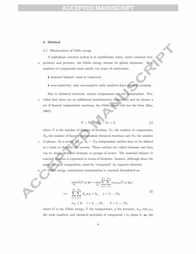
2. Method

2.1. Minimization of Gibbs energy

A multiphase reaction system is at equilibrium, when, under constant tem-

perature and pressure, the Gibbs energy attains its global minimum. Mole65

numbers of components must satisfy two types of constraints:

• material balance: mass is conserved

• non-negativity: only non-negative mole numbers have physical meaning

Due to chemical reactions, system components are not independent. Pro-

vided that there are no additional stoichiometric constraints and we choose a70

set of linearly independent reactions, the Gibbs phase rule has the form (Rao,

1985):

F = NC −NR −NP + 2 (1)

where F is the number of degrees of freedom, NC the number of components,

NR the number of linearly independent chemical reactions and NP the number

of phases. As a result, NE = NC −NR independent entities have to be defined75

as a basis to describe the system. These entities are called elements and they

can be single chemical elements or groups of atoms. The material balance in

reaction systems is expressed in terms of elements. Isomers, although share the

same chemical composition, must be “composed” by separate elements.

Gibbs energy constrained minimization is concisely formulated as:80

minnG(T, p,n) = min

nik

NP∑k=1

NC∑i=1

nikµik(T, p,nk)

s.t.

NP∑k=1

NC∑i=1

Ajinik = bj , j = 1, ..., NE

nik ≥ 0, i = 1, ..., NC k = 1, ..., NP

(2)

where G is the Gibbs energy, T the temperature, p the pressure, nik and µik

the mole numbers and chemical potential of component i in phase k, nk the

4

components abundance vector in phase k, Aji the number of element j in com-

ponent i and bj the total mole numbers of element j. The material balance in

the matrix-vector form is:85

A

NP∑k=1

nk = b (3)

where A is the formula matrix and b the element abundance vector. The latter

can be found from the single-phase feed mole numbers, nF :

b = AnF (4)

Chemical potential is calculated from:

µik = µ◦ik +RT lnfikf◦ik

(5)

where µ◦ik is the reference state chemical potential of component i in phase k,

R the gas constant, fik the fugacity of component i in phase k and f◦ik the90

reference state fugacity of component i in phase k.

If the same EoS is used for all phases, the ideal gas reference state is selected

at the temperature of the system: µ◦ik = µ∗i (T, p∗) and f◦ik = p∗, where p∗ is

usually 1 atm or 1 bar. If an activity coefficient model is used for liquid phases,

the pure component reference state is selected for those phases at the temper-95

ature and pressure of the system: µ◦ik = µpureik (T, p) and f◦ik = fik(T, p). The

subscript k is used in fik only to differentiate vapor and liquid pure component

fugacities. It is possible to change between the two reference states:

µ∗i − µpureik = RT ln

p∗

fik(6)

Fugacities are calculated from an EoS by:

fik = xikφikp (7)

where xik is the mole fraction of component i in phase k and φik the fugacity100

coefficient of component i in phase k. For a liquid phase described by an activity

5

coefficient model, fugacities are calculated by:

fik = xikγikfik (8)

where γik is the activity coefficient of component i in liquid phase k. An equiv-

alent fugacity coefficient is given by:

φik =γikfikp

(9)

At low pressures, for a liquid:105

fik = psi (10)

where psi is the vapor pressure of component i. It must be clarified that ideal

vapor phases behave like ideal gases (φ = 1), while ideal liquid phases behave

like ideal solutions (γ = 1).

Reactions between components Ai can be expressed as:

NC∑i=1

Aiνir = 0, r = 1, ..., NR (11)

where νir is the stoichiometric coefficient of component i in reaction r, positive110

for products and negative for reactants. With stoichiometric coefficients as

its entries, the stoichiometric matrix N is a complete representation of all the

reactions. The product of the formula matrix with the stoichiometric matrix

must satisfy:

AN = 0 (12)

Temperature is constant, hence the Gibbs energy has the same minimum as115

the reduced Gibbs energy, G/(RT ). The Lagrangian of the latter is:

L(n,λ) =

NP∑k=1

NC∑i=1

nikµik

RT−

NE∑j=1

λj

(NP∑k=1

NC∑i=1

Ajinik − bj

)(13)

6

where λj is the Lagrange multiplier of element j. The solution is a stationary

point of the Lagrangian, satisfying:

∂L∂nik

=µik

RT−

NE∑j=1

Ajiλj = 0, i = 1, ..., NC k = 1, ..., NP (14)

∂L∂λj

= −NP∑k=1

NC∑i=1

Ajinik + bj = 0, j = 1, ..., NE (15)

We must mention that this point is a saddle of the Lagrangian. The purpose

is not to minimize the Lagrangian, but the reduced Gibbs energy. Instead of120

solving this set of equations, we introduce the mole fractions and the phase

amounts in Eq. 15:

FAj =

NP∑k=1

nt,k

NC∑i=1

Ajixik − bj = 0, j = 1, ..., NE (16)

Mole fractions in each phase must also satisfy:

FBk =

NC∑i=1

xik − 1 = 0, k = 1, ..., NP (17)

From Eq. 5 and 14, the mole fraction can be expressed as a function of the

Lagrange multipliers:125

lnxik =

NE∑j=1

Ajiλj −µ◦ikRT− ln

φikp

f◦ik(18)

The working equations of the procedure are given by Eq. 16 and 17. The

independent variables at equilibrium, λ and nt, are roots of the function F:

F(λ,nt) =

FA

FB

(19)

To find the Jacobian of F, derivatives of xik are required. Whenever we use the

Jacobian in calculations, we assume that the fugacity coefficients are constant.

Therefore:130

∂xik∂λq

= Aqixik, q = 1, ..., NE (20)

7

and:

∂xik∂nt,q

= 0, q = 1, ..., NP (21)

Finally, the Jacobian matrix of function F has the form:

J(λ,nt) =

JA JB

JC JD

(22)

where:

JAjq =

∂FAj

∂λq=

NP∑k=1

nt,k

NC∑i=1

AjiAqixik, j = 1, ..., NE q = 1, ..., NE (23)

JBjq =

∂FAj

∂nt,q=

NC∑i=1

Ajixiq, j = 1, ..., NE q = 1, ..., NP (24)

JCkq =

∂FBk

∂λq=

NC∑i=1

Aqixik = JBqk, k = 1, ..., NP q = 1, ..., NE (25)

JDkq =

∂FBk

∂nt,q= 0, k = 1, ..., NP q = 1, ..., NP (26)

or

J(λ,nt) =

JA JB

(JB)T 0

(27)

The solution of F is determined iteratively with the Newton’s method:135

J

∆λ

∆nt

= −F (28)

A nested-loop scheme is employed: in the inner loop we keep constant the

values of fugacity or activity coefficients. When the estimate of Eq. 28 con-

verges, we update all non-ideality quantities in the outer loop. The dimensions

of the system in the inner loop is NE +NP . The original working equations (Eq.

8

14 and 15) require determining a total of NCNP + NE variables, whereas the140

nested-loop scheme uses (NC − 1)NP fewer variables. According to Eq. 14, a

relationship can be found between the minimum Gibbs energy and the Lagrange

multipliers:

Gmin

RT=

NP∑k=1

NC∑i=1

nikµik

RT=

NP∑k=1

NC∑i=1

nik

NE∑j=1

Ajiλj =

=

NE∑j=1

λj

NP∑k=1

NC∑i=1

Ajinik =

NE∑j=1

bjλj

(29)

Eq. 29 shows that the minimum Gibbs energy is a homogeneous function of

degree one in the mole numbers of the elements bj , therefore:145

(∂Gmin

∂bj

)T,p,bq 6=j

= RTλj (30)

In other words, the Lagrange multipliers represent the reduced chemical poten-

tial of the elements at equilibrium.

2.2. Initialization

To initialize calculations, usually a linear programming problem is solved

for non-zero mole numbers of NE components (Michelsen and Mollerup, 2007).150

From this solution we can determine estimates of λ and nt. Disadvantages

associated with this method are, except degenerate cases, the poor estimation of

small concentrations or the possibility that we find a solution with less than NE

components present. In this case, there is not enough information to determine

λ (Michelsen and Mollerup, 2007).155

To avoid solving this problem, we estimate the phase amounts and deter-

mine the Lagrange multipliers from an unconstrained minimization problem.

In general, it is easier to decide on a reasonable estimate for nt rather than

λ at equilibrium. We assume that the mole numbers of a single phase will be

between a minimum and a maximum value, due to reactions. In this work, the160

initial guess for nt was selected as the average of these two values. Although

generalization for a multiphase system is not addressed here, initial estimates of

9

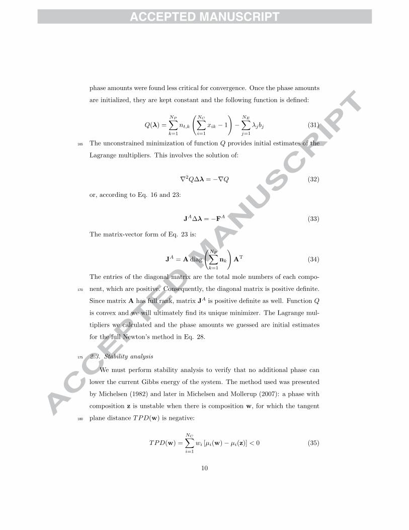
phase amounts were found less critical for convergence. Once the phase amounts

are initialized, they are kept constant and the following function is defined:

Q(λ) =

NP∑k=1

nt,k

(NC∑i=1

xik − 1

)−

NE∑j=1

λjbj (31)

The unconstrained minimization of function Q provides initial estimates of the165

Lagrange multipliers. This involves the solution of:

∇2Q∆λ = −∇Q (32)

or, according to Eq. 16 and 23:

JA∆λ = −FA (33)

The matrix-vector form of Eq. 23 is:

JA = A diag

(NP∑k=1

nk

)AT (34)

The entries of the diagonal matrix are the total mole numbers of each compo-

nent, which are positive. Consequently, the diagonal matrix is positive definite.170

Since matrix A has full rank, matrix JA is positive definite as well. Function Q

is convex and we will ultimately find its unique minimizer. The Lagrange mul-

tipliers we calculated and the phase amounts we guessed are initial estimates

for the full Newton’s method in Eq. 28.

2.3. Stability analysis175

We must perform stability analysis to verify that no additional phase can

lower the current Gibbs energy of the system. The method used was presented

by Michelsen (1982) and later in Michelsen and Mollerup (2007): a phase with

composition z is unstable when there is composition w, for which the tangent

plane distance TPD(w) is negative:180

TPD(w) =

NC∑i=1

wi [µi(w)− µi(z)] < 0 (35)

10

Negative values of TPD can be identified through determination of its min-

ima (Michelsen, 1982) and a phase split occurs if a negative TPD is found

during the search. Stability analysis for multiphase calculations is essentially

the same as for a two-phase system. Any phase of the converged solution can

be used to test the overall stability. However, special care needs to be taken for185

the initial estimates in multiphase calculation (Michelsen, 1982; Michelsen and

Mollerup, 2007).

2.4. Assignment of reference state chemical potential

The reference state chemical potential is needed to calculate mole fractions

from Eq. 18. It can be found in tables for specific T and p. Although necessary,190

this information is not always available. Instead, chemical equilibrium constants

are more frequently reported:

Keqrk = exp

(−∆rG

◦rk

RT

)= exp

(−

NC∑i=1

νirµ◦ik

RT

)(36)

where Keqrk is the chemical equilibrium constant of reaction r in phase k and

∆rG◦rk the reference state Gibbs energy of reaction r in phase k, which can

also be calculated based on the Gibss energy of formation or Gibbs energy of195

combustion.

In total NC reference state chemical potentials are missing from phase k, but

there are only NR chemical equilibrium constants. Absolute values of µ◦ik do not

matter for the calculations, as long as they satisfy Eq. 36. In place of the real

reference state chemical potential, we “decompose” the chemical equilibrium200

constants into fictitious, yet consistent, values: NR reference components are

selected, that participate in one reaction at least (no inerts) and we assign:

µ◦ik =

µik, i ∈ reference components

0, i 6∈ reference components

(37)

11

The following system is solved for µk/(RT ):

1

RTNTµk =

− lnKeq1k

.

.

.

− lnKeqrk

(38)

where N is the stoichiometric matrix of the NR reference components we chose.

When all phases share the same reference state, then µ◦ik = µ◦iq∣∣q 6=k

for all205

components. Otherwise, Eq. 6 must be used.

3. Results and discussion

In this work, Q function (Eq. 31) is minimized assuming a single ideal

phase. Afterwards, stability analysis provides the necessary composition esti-

mates, when an additional phase must be considered. Starting values for the210

Lagrange multipliers in the new phase set are taken from the previous solution

and nt,new phase = 0. The procedure stops when the maximum error in the in-

dependent variables (λ and nt) is less than 10−10. The error at iteration q ≥ 1

is calculated as:

error(q) =

√√√√NE∑j=1

[λ(q)j − λ

(q−1)j

]2+

NP∑k=1

[n(q)t,k − n

(q−1)t,k

]2(39)

Figure 1 summarizes the suggested procedure for solving CPE involving215

multiple phases and multiple reactions. It should be noted that this method is

intended to provide a general and safe solution. Therefore, calculations start

from a single phase and additional phases are introduced in a step-wise manner,

one at a time. It is possible to start calculations from more than one phases.

Although more risky, this might save time in actual calculation. Our trials220

have shown that the algorithm converges for most tested cases, even if initially

NP > 1. Nevertheless, this is not the focus of this work.

12

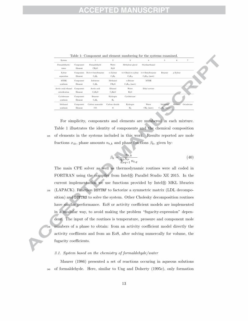
Table 1: Component and element numbering for the systems examined.

System 1 2 3 4 5 6 7

Formaldehyde/ Component Formaldehyde Water Methylene glycol Oxydimethanol

water Element CH2O H2O

Xylene Component Di-tert-butylbenzene m-Xylene tert-Butyl-m-xylene tert-Butylbenzene Benzene p-Xylene

separation Element C6H6 C4H8 C8H10 C8H10 (inert)

MTBE Component Isobutene Methanol n-Butane MTBE

synthesis Element C4H8 CH4O C4H10 (inert)

Acetic acid/ethanol Component Acetic acid Ethanol Water Ethyl acetate

esterification Element C2H2O C2H6O H2O

Cyclohexane Component Benzene Hydrogen Cyclohexane

synthesis Element C6H6 H2

Methanol Component Carbon monoxide Carbon dioxide Hydrogen Water Methanol Methane Octadecane

synthesis Element CO O H2 CH4 (inert) C18H38 (inert)

For simplicity, components and elements are numbered in each mixture.

Table 1 illustrates the identity of components and the chemical composition

of elements in the systems included in this work. Results reported are mole225

fractions xik, phase amounts nt,k and phase fractions βk, given by:

βk =nt,k∑NP

q=1 nt,q(40)

The main CPE solver as well as thermodynamic routines were all coded in

FORTRAN using the compiler from Intel R© Parallel Studio XE 2015. In the

current implementation we use functions provided by Intel R© MKL libraries

(LAPACK). Function DSYTRF to factorize a symmetric matrix (LDL decompo-230

sition) and DSYTRS to solve the system. Other Cholesky decomposition routines

have similar performance. EoS or activity coefficient models are implemented

in a modular way, to avoid making the problem “fugacity-expression” depen-

dent. The input of the routines is temperature, pressure and component mole

numbers of a phase to obtain: from an activity coefficient model directly the235

activity coeffiients and from an EoS, after solving numercally for volume, the

fugacity coefficients.

3.1. System based on the chemistry of formaldehyde/water

Maurer (1986) presented a set of reactions occuring in aqueous solutions

of formaldehyde. Here, similar to Ung and Doherty (1995e), only formation240

13

Set T , p, nF , NP = 1and guess nt

Find λ initial estimatesfrom the nt guess

Solve equationswith Newton’s method

All phasesideal? Update γ or φNP = NP + 1

Stable? Converged?

Get λ, nt and xk

yes no

yes no

yes

no

Figure 1: Flowchart of the reported algorithm.

of methylene glycol and oxydimethanol (dimer in polyoxymethylene polymer-

ization) are considered for the calculations. Formaldehyde reacts with water

to produce methylene glycol, which subsequently produces oxydimethanol in a

condensation dimerization:

CH2O + H2O ⇀↽ CH4O2 (41)

2CH4O2 ⇀↽ C2H6O3 + H2O (42)

The number of elements is NE = NC − NR = 4 − 2 = 2. The formula matrix245

and stoichiometric matrix of the system are given by:

A =

1 0 1 2

0 1 1 1

N =

−1 −1 1 0

0 1 −2 1

T

(43)

Vapor and liquid phases are considered ideal as in Ung and Doherty (1995e),

unlike in Maurer (1986), who used the UNIFAC activity coefficient model (Fre-

14

denslund et al., 1975) for the liquid phase. Chemical equilibrium constants and

vapor pressure expressions were taken from Maurer (1986). Oxydimethanol is250

considered non-volatile and consequently its concentration in the vapor phase is

zero. Both phases are ideal and as a result there are no non-reactive azeotropes.

Ung and Doherty (1995e) showed that there are no reactive azeotropes either.

Equilibrium T − y − x diagrams at 1 atm for all system components are pre-

sented in Figure 2. As mentioned in Ung and Doherty (1995e), reactions do255

not allow the concentration of every component to span the full range [0,1]. For

instance, it can be seen from Eq. 42, that a pure methylene glycol solution does

not exist, because pairs of these molecules produce dimers through condensa-

tion. Maximum methylene glycol in the vapor phase is less than 0.1% at 315.98

K. Maximum concentrations in the liquid phase are x3 = 0.24 at 304.07 K for260

methylene glycol and x4 = 0.60 at 285.02 K for oxydimethanol.

3.2. Xylene separation

Saito et al. (1971) examined the possibility of separating m- and p-xylene.

Normal distillation is not applicable, since isomers have close boiling points and

crystallization has certain limitations. They chose reactive distillation, taking265

advantage of the following reactions:

C14H22 +m - C8H10 ⇀↽ C12H18 + C10H14 (44)

C10H14 +m - C8H10 ⇀↽ C12H18 + C6H6 (45)

where di-tert-butylbenzene reacts withm-xylene to produce tert-butyl-m-xylene

and tert-butylbenzene, the latter reacting at the same time with m-xylene to

produce tert-butyl-m-xylene and benzene. In this reaction system, p-xylene is

an inert. The number of elements is NE = NC −NR = 6− 2 = 4. The formula270

15

0 0.2 0.4 0.6 0.8 1240

260

280

300

320

340

360

380

Formaldehyde mole fraction

Tem

pera

ture

(K)

L V

(a)

0 0.2 0.4 0.6 0.8 1240

260

280

300

320

340

360

380

Water mole fraction

Tem

pera

ture

(K)

L V

(b)

0 0.2 0.4 0.6 0.8 1240

260

280

300

320

340

360

380

Methylene glycol mole fraction

Tem

pera

ture

(K)

L V

(c)

0 0.2 0.4 0.6 0.8 1240

260

280

300

320

340

360

380

Oxydimethanol mole fraction

Tem

pera

ture

(K)

L V

(d)

Figure 2: Equilibrium T -y-x diagrams for formaldehyde (a), water (b), methylene glycol (c)

and oxydimethanol (d) at 1 atm.

16

Table 2: Mole fractions in xylene separation at the bubble point of 44 mmHg.

Component Feed Our work – 336.54 K Saito et al. (1971) – 331.15 K

Di-tert-butylbenzene

m-Xylene

tert-Butyl-m-xylene

tert-Butylbenzene

Benzene

p-Xylene

0.29

0.08

0.07

0.19

0.03

0.34

Vapor Liquid

0.01 0.29

0.10 0.08

0.01 0.07

0.08 0.19

0.34 0.03

0.47 0.34

Vapor

0.02

0.14

0.01

0.11

0.22

0.50

matrix and stoichiometric matrix of the system are given by:

A =

1 0 0 1 1 0

2 0 1 1 0 0

0 1 1 0 0 0

0 0 0 0 0 1

N =

−1 −1 1 1 0 0

0 −1 1 −1 1 0

T

(46)

Vapor and liquid phases are ideal. Chemical equilibrium constants and

vapor pressure expressions were taken from Saito et al. (1971). The authors

determined experimentally compositions at different plates in two distillation

columns: lower pressure alkylation column of m-xylene and higher pressure re-275

covery column of m-xylene and alkylating reagent. Bubble point calculations

are performed for the 1st plate/condenser of the column and compared with the

experimental compositions (Saito et al., 1971) in Tables 2 and 3. At both tem-

peratures, highest deviations are noted for benzene. In Figure 3, for the same

feed compositions, we present the temperature range of the 2-phase system, as280

well as the mole fractions of each component. Most mole fractions curves exhibit

monotonic behavior. Although xylene isomer compositions might have maxima

in the two different pressures and phases, p-xylene shows the clearest maximum

at 347.52 K and 44 mmHg with a vapor phase composition of y6 = 0.557.

17

Table 3: Mole fractions in xylene separation at the bubble point of 86 mmHg.

Component Feed Our work – 324.40 K Saito et al. (1971) – 323.15 K

Di-tert-butylbenzene

m-Xylene

tert-Butyl-m-xylene

tert-Butylbenzene

Benzene

p-Xylene

0.09

0.35

0.04

0.21

0.25

0.06

Vapor Liquid

0.00 0.07

0.13 0.34

0.00 0.05

0.03 0.24

0.82 0.24

0.02 0.06

Vapor

0.00

0.29

0.00

0.05

0.59

0.07

3.3. MTBE synthesis285

Ung and Doherty (1995e) studied the phase behavior of methyl-tert-butyl

ether (MTBE) synthesis from isobutene and methanol in the presence of n-

butane as an inert:

C4H8 + CH4O ⇀↽ C5H12O (47)

The number of elements is NE = NC − NR = 4 − 1 = 3. The formula matrix

and stoichiometric matrix of the system are given by:290

A =

1 0 0 1

0 1 0 1

0 0 1 0

N =[−1 −1 0 1

]T(48)

Vapor phase is considered ideal and liquid phase is described by the Wilson

activity coefficient model (Wilson, 1964). The chemical equilibrium constant,

vapor pressure expressions and parameters for the Wilson model were taken

from Ung and Doherty (1995e). At a reactive azeotrope, Ung and Doherty

(1995b) proved that mole fractions in the two phases are not necessarily equal.295

Instead, they introduce a set of transformed composition variables, denoted by

capital letters, which simplifies the analysis. According to their new notation,

at a reactive azeotrope X = Y for all reference components. For this system,

18

44 mmHg 86 mmHg

330 340 350 360 370 380 3900

0.2

0.4

0.6

0.8

1

Temperature (K)

Phas

efra

ctio

nL V

(a)

320 330 340 350 360 370 380 3900

0.2

0.4

0.6

0.8

1

Temperature (K)

Phas

efra

ctio

n

L V

(b)

330 340 350 360 370 380 3900

0.2

0.4

0.6

0.8

1

Temperature (K)

Mol

efra

ctio

n

y1 y2 y3y4 y5 y6

(c)

320 330 340 350 360 370 380 3900

0.2

0.4

0.6

0.8

1

Temperature (K)

Mol

efra

ctio

ny1 y2 y3y4 y5 y6

(d)

330 340 350 360 370 380 3900

0.2

0.4

0.6

0.8

1

Temperature (K)

Mol

efra

ctio

n

x1 x2 x3x4 x5 x6

(e)

320 330 340 350 360 370 380 3900

0.2

0.4

0.6

0.8

1

Temperature (K)

Mol

efra

ctio

n

x1 x2 x3x4 x5 x6

(f)

Figure 3: Phase fractions (a, b) and mole fractions (c, d, e, f) in xylene separation for the

feeds reported in Tables 2 and 3.

19

transformed compositions are found by:

X1 =x1 + x41 + x4

X2 =x2 + x41 + x4

X3 =x3

1 + x4(49)

For the derivation and the implications of transformed variables, the reader is300

referred to Ung and Doherty (1995b,d). The equilibrium diagrams at 1 atm

are presented in Figures 4a and 4b using transformed compositions. The inert

was not considered in these calculations. An “intermediate-boiling inflection

azeotrope” is identified, or according to Ung and Doherty (1995e), a “pseudo-

reactive azeotrope”, for being fairly close to the diagonal (Figure 4b). We305

observed this point at 320.92 K. In Figure 4c, we find that the maximum MTBE

concentrations are y4 = 0.70 in the vapor phase at 320.56 K and x4 = 0.93 in

the liquid phase at 317.70 K. The absence of the inert allows us to depict all

the equilibrium curves in two-dimensional diagrams.

We also examined the inert effect in the following conditions: 300 K and 1310

atm with an equimolar feed of reactants (isobutene and methanol, 1 mol each).

Different values of mole numbers for the inert were included in this feed and

the effects on the overall equilibrium are presented in Figure 5. Phase fractions

and mole fractions of all the components are shown, as the inert concentration

increases in the feed. The vapor pressure expression constants for n-butane315

were taken from NIST Chemistry WebBook (Accessed: 19.02.2016). Since the

inert is volatile, a vapor phase appears with the addition of approximately 0.36

mol of n-butane, after which the vapor phase fraction increases with n-butane

concentration until we obtain 100% vapor. The mole fraction of MTBE (Figure

5e) for a single phase decreases as the moles of the inert in the feed increase.320

In the two-phase region, the phase compositions of MTBE and n-butane (Fig-

ures 5d and 5e) change only slightly. However, the overall mole fraction of

MTBE (the total moles of MTBE divided by the total moles of the components

in the system) decreases continuously as a result of the dilution by the inert

component.325

20

0 0.2 0.4 0.6 0.8 1260

280

300

320

340

MTBE mole fraction

Tem

pera

ture

(K)

L V

(a)

0 0.2 0.4 0.6 0.8 1260

280

300

320

340

Y1, X1

Tem

pera

ture

(K)

L V

(b)

0 0.2 0.4 0.6 0.8 10

0.2

0.4

0.6

0.8

1

X

Y

Isobutene Methanol

(c)

Figure 4: Equilibrium T -y-x diagram for MTBE (a), T -Y -X diagram for isobutene (b) and

Y -X diagram for isobutene and methanol (c) in MTBE synthesis at 1 atm.

21

0 0.5 1 1.5 2 2.5 30

0.2

0.4

0.6

0.8

1

Feed n-butane (mol)

Phas

efra

ctio

n

V L

(a)

0 0.5 1 1.5 2 2.5 30

0.02

0.04

0.06

0.08

0.1

Feed n-butane (mol)

Isob

uten

em

ole

fract

ion

V L Overall

(b)

0 0.5 1 1.5 2 2.5 30

0.02

0.04

0.06

0.08

0.1

Feed n-butane (mol)

Met

hano

lmol

efra

ctio

nV L Overall

(c)

0 0.5 1 1.5 2 2.5 30

0.2

0.4

0.6

0.8

1

Feed n-butane (mol)

n-B

utan

em

ole

fract

ion

V L Overall

(d)

0 0.5 1 1.5 2 2.5 30

0.2

0.4

0.6

0.8

1

Feed n-butane (mol)

MT

BEm

ole

fract

ion

V L Overall

(e)

Figure 5: Phase fractions (a), mole fractions of isobutene (b), methanol (c), n-butane (d) and

MTBE (e) as a function of n-butane moles in the feed for the MTBE synthesis at 300 K and

1 atm.

22

3.4. Esterification of acetic acid and ethanol

One of the most studied esterification reactions is between acetic acid and

ethanol producing ethyl acetate and water:

C2H4O2 + C2H6O ⇀↽ C4H8O2 + H2O (50)

The number of elements is NE = NC − NR = 4 − 1 = 3. The formula matrix

and stoichiometric matrix of the system are given by:330

A =

1 0 0 1

0 1 0 1

1 0 1 0

N =[−1 −1 1 1

]T(51)

Vapor phase is considered ideal and liquid phase is described by the UNI-

QUAC activity coefficient model (Abrams and Prausnitz, 1975). The chemical

equilibrium constant, vapor pressure expressions and parameters for the UNI-

QUAC model were taken from Xiao et al. (1989). Castier et al. (1989) stud-

ied this system including the competing etherification reaction of ethanol to335

diethylether as well as the dimerization of acetic acid in the vapor phase. Com-

parisons are made with the results of Xiao et al. (1989), and Stateva and Wake-

ham (1997) in Table 4. Larger deviations with Stateva and Wakeham (1997)

could be attributed to selecting a different source for the chemical equilibrium

constant. In Figure 6, phase boundaries and mole fractions are presented for an340

equimolar feed of the reactants.

3.5. Cyclohexane synthesis

George et al. (1976) examined the hydrogenation of benzene at high tem-

perature for cyclohexane synthesis:

C6H6 + 3H2 ⇀↽ C6H12 (52)

23

346 348 350 352 354 356 3580

0.2

0.4

0.6

0.8

1

Temperature (K)

Phas

efra

ctio

nL V

(a)

346 348 350 352 354 356 3580

0.2

0.4

0.6

0.8

1

Temperature (K)

Mol

efra

ctio

n

y1 y2 y3 y4

(b)

346 348 350 352 354 356 3580

0.2

0.4

0.6

0.8

1

Temperature (K)

Mol

efra

ctio

n

x1 x2 x3 x4

(c)

Figure 6: Phase fractions (a) and mole fractions (b, c) in acetic acid/ethanol esterification for

an equimolar feed of reactants at 1 atm.

24

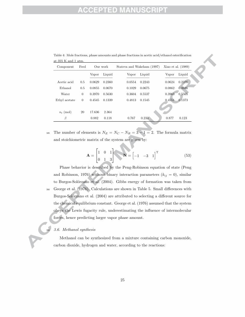
Table 4: Mole fractions, phase amounts and phase fractions in acetic acid/ethanol esterification

at 355 K and 1 atm.

Component Feed Our work Stateva and Wakeham (1997) Xiao et al. (1989)

Acetic acid

Ethanol

Water

Ethyl acetate

nt (mol)

β

0.5

0.5

0

0

20

Vapor Liquid

0.0629 0.2360

0.0855 0.0670

0.3970 0.5630

0.4545 0.1339

17.636 2.364

0.882 0.118

Vapor Liquid

0.0554 0.2243

0.1029 0.0675

0.3604 0.5537

0.4813 0.1545

0.767 0.233

Vapor Liquid

0.0624 0.2376

0.0862 0.0686

0.3963 0.5565

0.4551 0.1373

0.877 0.123

The number of elements is NE = NC − NR = 3 − 1 = 2. The formula matrix345

and stoichiometric matrix of the system are given by:

A =

1 0 1

0 1 3

N =[−1 −3 1

]T(53)

Phase behavior is described by the Peng-Robinson equation of state (Peng

and Robinson, 1976) without binary interaction parameters (kij = 0), similar

to Burgos-Solorzano et al. (2004). Gibbs energy of formation was taken from

George et al. (1976). Calculations are shown in Table 5. Small differences with350

Burgos-Solorzano et al. (2004) are attributed to selecting a different source for

the chemical equilibrium constant. George et al. (1976) assumed that the system

obeys the Lewis fugacity rule, underestimating the influence of intermolecular

forces, hence predicting larger vapor phase amount.

3.6. Methanol synthesis355

Methanol can be synthesized from a mixture containing carbon monoxide,

carbon dioxide, hydrogen and water, according to the reactions:

25

Table 5: Mole fractions, phase amounts and phase fractions in cyclohexane synthesis at 500

K and 30 atm.

Component Feed Our work Burgos-Solorzano et al. (2004) George et al. (1976)

Benzene

Hydrogen

Cyclohexane

nt (mol)

β

0.247

0.753

0

4.05

Vapor Liquid

4.45× 10−6 5.43× 10−6

0.238 0.0204

0.762 0.980

0.132 0.918

0.125 0.875

Vapor Liquid

4.00× 10−6 4.92× 10−6

0.249 0.0147

0.751 0.985

0.148 0.902

0.141 0.859

Vapor Liquid

3.64× 10−4 3.87× 10−4

0.076 0.0023

0.923 0.997

0.660 0.391

0.628 0.372

CO + 2H2 ⇀↽ CH4O (54)

CO2 + H2 ⇀↽ CO + H2O (55)

Methane and octadecane are included as inerts. The number of elements is

NE = NC −NR = 7− 2 = 5. The formula matrix and stoichiometric matrix of

the system are given by:360

A =

1 1 0 0 1 0 0

0 1 0 1 0 0 0

0 0 1 1 2 0 0

0 0 0 0 0 1 0

0 0 0 0 0 0 1

N =

−1 0 −2 0 1 0 0

1 −1 −1 1 0 0 0

T

(56)

Phase behavior is described by the Soave-Redlich-Kwong equation of state

(Soave, 1972) with binary interaction parameters kij from Castier et al. (1989).

Ideal gas chemical potentials at 1 bar (reference state) were taken from Phoenix

and Heidemann (1998). In Tables 6 and 7, two different feeds are used to

produce methanol, resulting in a 2- and 3-phase system respectively. Results365

from Stateva and Wakeham (1997), and Castier et al. (1989) are also included

for comparison. Introduction of the heavy hydrocarbon results in two immiscible

liquid phases along with the vapor phase. For identification purposes, we named

26

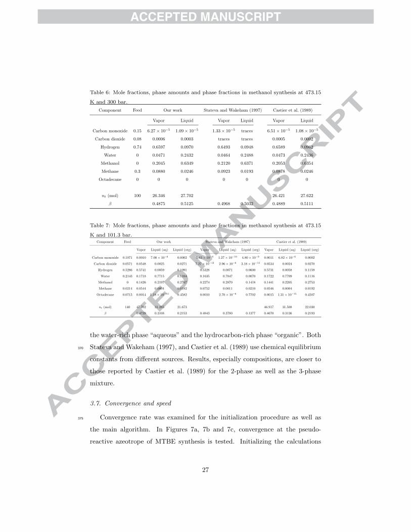
Table 6: Mole fractions, phase amounts and phase fractions in methanol synthesis at 473.15

K and 300 bar.

Component Feed Our work Stateva and Wakeham (1997) Castier et al. (1989)

Carbon monoxide

Carbon dioxide

Hydrogen

Water

Methanol

Methane

Octadecane

nt (mol)

β

0.15

0.08

0.74

0

0

0.3

0

100

Vapor Liquid

6.27× 10−5 1.09× 10−5

0.0006 0.0003

0.6597 0.0970

0.0471 0.2432

0.2045 0.6349

0.0880 0.0246

0 0

26.346 27.702

0.4875 0.5125

Vapor Liquid

1.33× 10−5 traces

traces traces

0.6493 0.0948

0.0464 0.2488

0.2120 0.6371

0.0923 0.0193

0 0

0.4968 0.5032

Vapor Liquid

6.51× 10−5 1.08× 10−5

0.0005 0.0002

0.6589 0.0962

0.0473 0.2436

0.2053 0.6354

0.0878 0.0246

0 0

26.421 27.622

0.4889 0.5111

Table 7: Mole fractions, phase amounts and phase fractions in methanol synthesis at 473.15

K and 101.3 bar.Component Feed Our work Stateva and Wakeham (1997) Castier et al. (1989)

Carbon monoxide

Carbon dioxide

Hydrogen

Water

Methanol

Methane

Octadecane

nt (mol)

β

0.1071

0.0571

0.5286

0.2143

0

0.0214

0.0715

140

Vapor Liquid (aq) Liquid (org)

0.0010 7.00× 10−6 0.0002

0.0548 0.0025 0.0271

0.5741 0.0059 0.1091

0.1718 0.7715 0.1104

0.1426 0.2197 0.2767

0.0544 0.0004 0.0182

0.0014 1.18× 10−14 0.4582

47.702 31.285 21.673

0.4739 0.3108 0.2153

Vapor Liquid (aq) Liquid (org)

5.63× 10−8 1.27× 10−10 4.80× 10−9

7.27× 10−12 2.96× 10−6 3.18× 10−12

0.5328 0.0071 0.0600

0.1635 0.7047 0.0070

0.2274 0.2870 0.1418

0.0752 0.0011 0.0210

0.0010 2.70× 10−6 0.7702

0.4843 0.3780 0.1377

Vapor Liquid (aq) Liquid (org)

0.0011 6.82× 10−6 0.0002

0.0534 0.0024 0.0270

0.5731 0.0058 0.1159

0.1722 0.7709 0.1116

0.1441 0.2205 0.2753

0.0546 0.0004 0.0192

0.0015 1.31× 10−15 0.4507

46.917 31.508 22.030

0.4670 0.3136 0.2193

the water-rich phase “aqueous” and the hydrocarbon-rich phase “organic”. Both

Stateva and Wakeham (1997), and Castier et al. (1989) use chemical equilibrium370

constants from different sources. Results, especially compositions, are closer to

those reported by Castier et al. (1989) for the 2-phase as well as the 3-phase

mixture.

3.7. Convergence and speed

Convergence rate was examined for the initialization procedure as well as375

the main algorithm. In Figures 7a, 7b and 7c, convergence at the pseudo-

reactive azeotrope of MTBE synthesis is tested. Initializing the calculations

27

follows a quadratic convergence rate (minimization of Q function, Eq. 31). The

single-phase reaction requires a small number of iterations. Stability identifies

that a second phase will decrease the Gibbs energy and the 2-phase system380

requires almost three times as many iterations as the single-phase. A more

complete description of the convergence in this system is given by the inner loop

iterations for each outer loop non-ideality update. The closer to the solution

we are, the fewer Newton iterations are required for the inner loop convergence.

For cyclohexane synthesis in Figure 7d, fewer components result in a smaller385

number of iterations. Convergence for the system with the largest number

of components and phases, methanol synthesis, is presented in Figure 7e. In

contrast to the previous systems, the number of total iterations decreases with

the number of phases present in the system. Methanol single-phase synthesis

required the maximum number of iterations for all the systems in this work. In390

general, the iteration number is sensible, especially when it concerns a linearly

convergent procedure. It has to be noted that none of the calculations failed to

find the equilibrium compositions. As a result, the algorithm is robust, even for

computationally demanding VLE or VLLE of non-ideal systems.

The total CPU time required to determine the equilibrium of the systems395

for selected conditions is reported in Table 8. This time corresponds to the

complete procedure including initialization, solving CPE and stability analysis

(called after every time a phase set converges). It must be stressed that the time

spent to determine the solution is implementation and thermodynamic model

dependent for a specific system. For instance, more complex EoS are expected400

to result in slower calculations compared with a cubic EoS, as PR or SRK. The

fastest calculations are for ideal systems, where the outer loop (non-ideality

update) is not needed.

For the chemical and phase equilibrium calculation algorithms in the litera-

ture, their computational efficiencies are often reported in terms of CPU times405

and/or iteration numbers. However, it is not always straightforward to com-

pare various algorithms based on these performance indices, because they can

be influenced by many factors: The CPU times depend on the hardware, the

28

0 2 4 6 8 10

−12

−10

−8

−6

−4

−2

0

2

Iterations

log 1

0(er

ror)

(a)

0 4 8 12 16 20 24 28 32−12

−10

−8

−6

−4

−2

0

2

Iterations

log 1

0(er

ror)

L VL

(b)

0 4 8 12 16 20 24 28 320

1

2

3

4

5

6

7

Outer loop iteration index

Inne

rlo

opite

ratio

ns

L VL

(c)

0 4 8 12 16 20−12

−10

−8

−6

−4

−2

0

2

Iterations

log 1

0(er

ror)

V VL

(d)

0 8 16 24 32 40 48 56−12

−10

−8

−6

−4

−2

0

2

Iterations

log 1

0(er

ror)

V VL VLL

(e)

Figure 7: Convergence behavior of MTBE synthesis at 320.92 K and 1 atm

(isobutene/methanol 1:1.1) for Q function minimization (a) overall CPE (b), and inner loop

(Newton) iterations per outer loop non-ideality updates (c), cyclohexane synthesis at 500 K

and 30 atm (d), and 3-phase methanol synthesis at 473.15 K and 101.3 bar (e).

29

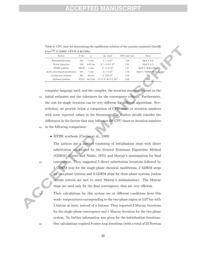
Table 8: CPU time for determining the equilibrium solution of the systems examined (Intel R©

CoreTM i7-5500U CPU@ 2.40 GHz).

System T (K) p nF (mol) CPU time (ms) Notes

Formaldehyde/water 310 1 atm [1 1 0 0]T 1.28 Ideal V & L

Xylene separation 350 0.05 atm [1 1 0 0 0 1]T 1.31 Ideal V & L

MTBE synthesis 320.92 1 atm [1 1.1 0 0]T 1.87 Ideal V, Wilson for L

Acetic acid/ethanol esterification 355 1 atm [1 1 0 0]T 1.72 Ideal V, UNIQUAC for L

Cyclohexane synthesis 500 30 atm [1 3.05 0]T 1.48 PR

Methanol synthesis 473.15 101.3 bar [15 8 74 30 3 0 10]T 3.08 SRK

computer language used, and the compiler; the iteration numbers depend on the

initial estimates and the tolerances for the convergence criteria. Furthermore,410

the cost for single iteration can be very different for different algorithms. Nev-

ertheless, we provide below a comparison of CPU times or iteration numbers

with some reported values in the literature. The readers should consider the

differences in the factors that may influence the CPU times or iteration numbers

in the following comparison:415

• MTBE synthesis (Castier et al., 1989)

The authors use a method consisting of initialization steps with direct

substitution accelerated by the General Dominant Eigenvalue Method

(GDEM) (Crowe and Nishio, 1975) and Murray’s minimization for final

convergence. They suggested 5 direct substitution iterations followed by420

1 GDEM step for the single-phase chemical equilibrium, 2 GDEM steps

for two-phase systems and 3 GDEM steps for three-phase systems (unless

certain criteria are met to enter Murray’s minimization). The Murray

steps are used only for the final convergence, thus are very efficient.

Their calculations for this system are at different conditions from this425

work: temperatures corresponding to the two-phase region at 5.07 bar with

1-butene as inert, instead of n-butane. They reported 2 Murray iterations

for the single-phase convergence and 1 Murray iteration for the two-phase

system. No further information was given for the initialization iterations.

Our calculations required 9 outer loop iterations (with a total of 25 Newton430

30

iterations) to converge the liquid phase and 30 outer loop iterations (with

a total of 73 Newton iterations) to converge the vapor-liquid system. The

authors can reach quadratic convergence rates, and therefore their method

is expected to be faster than the algorithm presented here.

• Cyclohexane synthesis (Burgos-Solorzano et al., 2004)435

The authors use a validation tool, a deterministic mathematical method

that guarantees finding the global minimum of the Gibbs energy. They

reported 120 ms required for the validation tool calculations [Sun Blade

1000 Model 1600 (600 MHz) workstation], whereas we spent 1.5 ms for the

complete calculations (initialization, convergence of single phase, stability440

analysis, convergence of two-phase system and final stability analysis).

• Acetic acid/ethanol esterification (Xiao et al., 1989; Castier et al., 1989)

Xiao et al. (1989) compared two stoichiometric methods, the S-C and the

KZ algorithm. The S-C algorithm is the classical stoichiometric approach

using nested loops. Its inner loop solves the phase equilibrium problem445

(flash) using a successive substitution approach based on the Rachford-

Rice equation, while its outer loop updates the extents of reaction. The

KZ algorithm, proposed as an improvement of the S-C algorithm, switches

the outer and inner loops in the S-C algorithm. They reported 10 outer

loop iterations (with a total of 42 Newton iterations) for the S-C algorithm450

and 9 outer loop iterations (with a total of 23 Newton iterations) for the

KZ algorithm. In our work, after 8 Newton iterations of the initialization

procedure, the solution obtained coincides with the single vapor phase

solution and the main solver was not needed. For the VLE of this reaction

system we needed 44 outer loop iterations (with a total of 106 Newton455

iterations). In Xiao et al. (1989), the initial assumption is a two-phase

system. Since all the three algorithms (S-C, KZ and ours) are supposed

to show an overall linear convergence, their iteration numbers should in

principle be comparable. We note that in Xiao et al. (1989) a very loose

tolerance is used for the convergence,∑NC

i=1(knewi /ki − 1)2 < 10−6, where460

31

ki = yi/xi. In our solution, a much tighter convergence criterion is used

(Eq. 39).

Castier et al. (1989) used a slightly higher temperature than the one pre-

sented in this work: 358.15 K. The ideal gas assumption for the vapor

phase resulted in a single vapor phase at equilibrium that required 3 Mur-465

ray iterations. On the other hand, using an EoS that accounts for the acid

dimerization in the vapor phase, convergence required 3 Murray iterations

for the initially assumed single vapor phase and 2 Murray iterations for

the final vapor-liquid system.

• Methanol synthesis (Castier et al., 1989)470

For the three-phase synthesis, all phase sets are initialized in Castier et al.

(1989): L, VL and VLL required 5 iterations with 1 GDEM step, 10

iterations with 2 GDEM steps, and 12 iterations with 2 GDEM steps

respectively (the third GDEM step was not needed for the three-phase

convergence). The Murray iterations to converge L, VL and VLL systems475

were 3, 4 and 1 respectively. We needed 10 Newton iterations for the

initialization of the single-phase system, and after stability introduced

additional phases, we did not initialize again. For our CPE calculations,

we needed 54 outer loop iterations (with a total of 149 Newton iterations)

for V, 27 outer loop iterations (with a total of 78 Newton iterations) for480

VL and 22 outer loop iterations (with a total of 60 Newton iterations) for

VLL. In our algorithm, no acceleration was implemented.

3.8. Alternative treatment

We have minimized Q function (Eq. 31) for a single ideal phase to ini-

tialize λ for the nested-loop calculations, by keeping the phase amount at a485

fixed value. Alternatively, this minimization could be attempted considering a

set of non-ideal phases (NP > 1), where the fugacity/activity coefficients are

assumed composition independent. Every time a new phase is introduced, fu-

gacity/activity coefficients are calculated for the current composition estimate

32

and kept constant during the minimization. Because ∇2Q is still positive def-490

inite, finding the unique minimizer is a safe procedure that requires a finite

number of iterations.

To reduce the number of iterations, an accelerated successive substitution

method could be utilized. The General Dominant Eigenvalue Method (GDEM)

(Crowe and Nishio, 1975) is a possible candidate. Although acceleration is495

needed to enhance the efficiency of calculations, the material balance is one of

the working equations, meaning that the independent variables do not obey it

at every iteration. As a result, the values of G = f(λ,nt) cannot be used to

validate, if the acceleration actually leads to a decrease in the Gibbs energy.

The RAND approach (White et al., 1958; Greiner, 1991; Michelsen and500

Mollerup, 2007) can also be used to increase the convergence rate. The method

of Lagrange multipliers discussed in this work can be employed as initial converg-

ing steps, before switching to the quadratically convergent RAND algorithm.

We will discuss how to apply the RAND approach to non-ideal multiphase and

multiple reaction systems in a separate paper.505

In a completely different formulation of the problem, the Gibbs energy is

minimized with respect to extents of reactions ξr under the non-negativity con-

straint:

minξG(T, p, ξ)

s.t. nik ≥ 0, i = 1, ..., NC k = 1, ..., NP

(57)

where

NP∑k=1

nik = nF,i +

NR∑r=1

νirξr (58)

If we do not account directly for the non-negativity constraints, this formulation510

is essentially an unconstrained minimization problem and can be advantageous

for a small number of reactions. However, there are initialization problems and

the method is prone to round-off errors. To overcome this obstacle, we can select

NE components as the “optimum” basis, the primary components, which are

33

the most abundant in the system (Michelsen and Mollerup, 2007). The rest of515

the components are called secondary and their mole numbers can be found from

those of the primary components. A number of publications has addressed the

issue of selecting the proper basis (Brinkley, 1946, 1947; Prigogine and Defay,

1947; Schott, 1964). The conventional treatment involves the solution of a PT-

flash in a nested loop and the update of the extents of the reactions in the outer520

loop. Two different stoichiometric algorithms are given in Castier et al. (1989),

and Phoenix and Heidemann (1998).

4. Conclusions

An extended algorithm for simultaneous chemical and phase equilibrium

calculations based on Michelsen (1989) and Michelsen and Mollerup (2007) was525

presented. The procedure involves a nested-loop scheme and calculations begin

by assuming a single-phase reaction system. The initialization method allows

for better quality initial estimates, while stability analysis guarantees finding the

Gibbs energy global minimum, by sequentially introducing new phases that can

lower the system Gibbs energy. CPE was successfully calculated for a number530

of systems described by different thermodynamic models. The convergence rate

is linear, due to the successive substitution in the outer loop. Nevertheless, the

method appears to be robust, without failing solving CPE for all the systems

examined.

Acknowledgments535

We would like to acknowledge the help of Prof. Michael L. Michelsen for his

insightful comments and suggestions.

References

Abrams, D.S., Prausnitz, J.M., 1975. Statistical thermodynamics of liquid mix-

tures: A new expression for the excess gibbs energy of partly or completely540

miscible systems. AIChE Journal 21, 116–128.

34

Barbosa, D., Doherty, M.F., 1988. The influence of equilibrium chemical re-

actions on vapor-liquid phase diagrams. Chemical Engineering Science 43,

529–540.

Bonilla-Petriciolet, A., Rangaiah, G.P., Segovia-Hernandez, J.G., 2011. Con-545

strained and unconstrained Gibbs free energy minimization in reactive sys-

tems using genetic algorithm and differential evolution with tabu list. Fluid

Phase Equilibria 300, 120–134.

Bonilla-Petriciolet, A., Segovia-Hernandez, J.G., 2010. A comparative study of

particle swarm optimization and its variants for phase stability and equilib-550

rium calculations in multicomponent reactive and non-reactive systems. Fluid

Phase Equilibria 289, 110–121.

Bonilla-Petriciolet, A., Vazquez-Roman, R., Iglesias-Silva, G.A., Hall, K.R.,

2006. Performance of stochastic global optimization methods in the calcula-

tion of phase stability analyses for nonreactive and reactive mixtures. Indus-555

trial & Egineering Chemistry Research 45, 4764–4772.

Brinkley, Jr, S.R., 1946. Note on the conditions of equilibrium for systems of

many constituents. The Journal of Chemical Physics 14, 563–564.

Brinkley, Jr, S.R., 1947. Calculation of the equilibrium composition of systems

of many constituents. The Journal of Chemical Physics 15, 107–110.560

Burgos-Solorzano, G.I., Brennecke, J.F., Stadtherr, M.A., 2004. Validated com-

puting approach for high-pressure chemical and multiphase equilibrium. Fluid

Phase Equilibria 219, 245–255.

Castier, M., Rasmussen, P., Fredenslund, A., 1989. Calculation of simultaneous

chemical and phase equilibria in nonideal systems. Chemical Engineering565

Science 44, 237–248.

Crowe, C.M., Nishio, M., 1975. Convergence promotion in the simulation of

chemical processes - the general dominant eigenvalue method. AIChE Journal

21, 528–533.

35

Floudas, C.A., Visweswaran, V., 1990. A global optimization algorithm (GOP)570

for certain classes of nonconvex NLPs–I. Theory. Computers & Chemical

Engineering 14, 1397–1417.

Fredenslund, A., Jones, R.L., Prausnitz, J.M., 1975. Group-contribution esti-

mation of activity coefficients in nonideal liquid mixtures. AIChE Journal 21,

1086–1099.575

Gautam, R., Seider, W.D., 1979a. Computation of phase and chemical equi-

librium: Part I. Local and constrained minima in Gibbs free energy. AIChE

Journal 25, 991–999.

Gautam, R., Seider, W.D., 1979b. Computation of phase and chemical equilib-

rium: Part II. Phase-splitting. AIChE Journal 25, 999–1006.580

Gautam, R., Seider, W.D., 1979c. Computation of phase and chemical equilib-

rium: Part III. Electrolytic solutions. AIChE Journal 25, 1006–1015.

Gautam, R., Wareck, J.S., 1986. Computation of physical and chemical

equilibria–alternate specifications. Computers & Chemical Engineering 10,

143–151.585

George, B., Brown, L.P., Farmer, C.H., Buthod, P., Manning, F.S., 1976. Com-

putation of multicomponent, multiphase equilibrium. Industrial & Engineer-

ing Chemistry Process Design and Development 15, 372–377.

Greiner, H., 1991. An efficient implementation of Newton’s method for complex

nonideal chemical equilibria. Computers & Chemical Engineering 15, 115–590

123.

Jalali, F., Seader, J.D., Khaleghi, S., 2008. Global solution approaches in equi-

librium and stability analysis using homotopy continuation in the complex

domain. Computers & Chemical Engineering 32, 2333–2345.

Jalali-Farahani, F., Seader, J.D., 2000. Use of homotopy-continuation method595

in stability analysis of multiphase, reacting systems. Computers & Chemical

Engineering 24, 1997–2008.

36

Maurer, G., 1986. Vapor-liquid equilibrium of formaldehyde-and water-

containing multicomponent mixtures. AIChE Journal 32, 932–948.

McDonald, C.M., Floudas, C.A., 1995. Global optimization for the phase and600

chemical equilibrium problem: Application to the NRTL equation. Computers

& Chemical Engineering 19, 1111–1139.

McDonald, C.M., Floudas, C.A., 1997. GLOPEQ: A new computational tool

for the phase and chemical equilibrium problem. Computers & Chemical

Engineering 121, 1–23.605

Michelsen, M.L., 1982. The isothermal flash problem. Part I. Stability. Fluid

Phase Equilibria 9, 1–19.

Michelsen, M.L., 1989. Calculation of multiphase ideal solution chemical equi-

librium. Fluid Phase Equilibria 53, 73–80.

Michelsen, M.L., Mollerup, J.M., 2007. Thermodynamic Models: Fundamen-610

tals & Computational Aspects. Second ed., Tie-Line Publications, Holte,

Denmark.

Moodley, K., Rarey, J., Ramjugernath, D., 2015. Application of the bio-inspired

Krill Herd optimization technique to phase equilibrium calculations. Com-

puters & Chemical Engineering 74, 75–88.615

NIST Chemistry WebBook, Accessed: 19.02.2016. NIST Standard Refer-

ence Database Number 69. http://webbook.nist.gov/cgi/cbook.cgi?ID=

C106978&Mask=4.

Peng, D.Y., Robinson, D.B., 1976. A new two-constant equation of state. In-

dustrial & Engineering Chemistry Fundamentals 15, 59–64.620

Perez Cisneros, E.S., Gani, R., Michelsen, M.L., 1997. Reactive separation

systems–I. Computation of physical and chemical equilibrium. Chemical En-

gineering Science 52, 527–543.

37

Phoenix, A.V., Heidemann, R.A., 1998. A non-ideal multiphase chemical equi-

librium algorithm. Fluid Phase Equilibria 150–151, 255–265.625

Prigogine, I., Defay, R., 1947. On the number of independent constituents and

the phase rule. The Journal of Chemical Physics 15, 614–615.

Rao, Y.K., 1985. Extended form of the Gibbs phase rule. Chemical Engineering

Education 19, 46–49.

Saito, S., Michishita, T., Maeda, S., 1971. Separation of meta- and para-xylene630

mixture by distillation accompanied by chemical reactions. Journal of Chem-

ical Engineering of Japan 4, 37–43.

Schott, G.L., 1964. Computation of restricted equilibria by general methods.

The Journal of Chemical Physics 40, 2065–2066.

Smith, W.R., Missen, R.W., 1982. Chemical Reaction Equilibrium Analysis:635

Theory and Algorithms. Wiley, New York, United States of America.

Soave, G., 1972. Equilibrium constants from a modified Redlich-Kwong equation

of state. Chemical Engineering Science 27, 1197–1203.

Stateva, R.P., Wakeham, W.A., 1997. Phase equilibrium calculations for chem-

ically reacting systems. Industrial & Engineering Chemistry Research 36,640

5474–5482.

Ung, S., Doherty, M.F., 1995a. Calculation of residue curve maps for mix-

tures with multiple equilibrium chemical reactions. Industrial & Engineering

Chemistry Research 34, 3195–3202.

Ung, S., Doherty, M.F., 1995b. Necessary and sufficient conditions for reactive645

azeotropes in multireaction mixtures. AIChE Journal 41, 2383–2392.

Ung, S., Doherty, M.F., 1995c. Synthesis of reactive distillation systems with

multiple equilibrium chemical reactions. Industrial & Engineering Chemistry

Research 34, 2555–2565.

38

Ung, S., Doherty, M.F., 1995d. Theory of phase equilibria in multireaction650

systems. Chemical Engineering Science 50, 3201–3216.

Ung, S., Doherty, M.F., 1995e. Vapor-liquid phase equilibrium in systems with

multiple chemical reactions. Chemical Engineering Science 50, 23–48.

Wasylkiewicz, S.K., Ung, S., 2000. Global phase stability analysis for hetero-

geneous reactive mixtures and calculation of reactive liquid-liquid and vapor-655

liquid-liquid equilibria. Fluid Phase Equilibria 175, 253–272.

White, III, C.W., Seider, W.D., 1981. Computation of phase and chemical

equilibrium: Part IV. Approach to chemical equilibrium. AIChE Journal 27,

466–471.

White, W.B., Johnson, S.M., Dantzig, G.B., 1958. Chemical equilibrium in660

complex mixtures. The Journal of Chemical Physics 28, 751–755.

Wilson, G.M., 1964. Vapor-liquid equilibrium. xi. a new expression for the

excess free energy of mixing. Journal of the American Chemical Society 86,

127–130.

Xiao, W.d., Zhu, K.h., Yuan, W.k., Chien, H.H.y., 1989. An algorithm for665

simultaneous chemical and phase equilibrium calculation. AIChE Journal 35,

1813–1820.

Zeleznik, F.J., Gordon, S., 1968. Calculation of complex chemical equilibria.

Industrial & Engineering Chemistry 60, 27–57.

39

Highlights

Equilibrium calculation of multiphase systems in presence of chemical reactions

Robust variable initialization and stability analysis for equilibrium verification

Successful calculations of two- and three-phase reaction systems

Coupling with a second-order method can improve computation efficiency