General rights Copyright and moral rights for the publications made accessible in the public portal are retained by the authors and/or other copyright owners and it is a condition of accessing publications that users recognise and abide by the legal requirements associated with these rights.

Users may download and print one copy of any publication from the public portal for the purpose of private study or research.

You may not further distribute the material or use it for any profit-making activity or commercial gain

You may freely distribute the URL identifying the publication in the public portal If you believe that this document breaches copyright please contact us providing details, and we will remove access to the work immediately and investigate your claim.

Downloaded from orbit.dtu.dk on: Mar 14, 2022

Calculation of Multiphase Chemical Equilibrium by the Modified RAND Method

Tsanas, Christos; Stenby, Erling Halfdan; Yan, Wei

Published in:Industrial and Engineering Chemistry Research

Link to article, DOI:10.1021/acs.iecr.7b02714

Publication date:2017

Document VersionPeer reviewed version

Link back to DTU Orbit

Citation (APA):Tsanas, C., Stenby, E. H., & Yan, W. (2017). Calculation of Multiphase Chemical Equilibrium by the ModifiedRAND Method. Industrial and Engineering Chemistry Research, 56(41), 11983-11995.https://doi.org/10.1021/acs.iecr.7b02714

Calculation of Multiphase Chemical

Equilibrium by the Modified RAND Method

Christos Tsanas, Erling H. Stenby, and Wei Yan∗

Center for Energy Resources Engineering (CERE), Department of Chemistry, Technical

University of Denmark, 2800 Kongens Lyngby, Denmark

E-mail: weya@kemi.dtu.dk

Abstract

A robust and efficient algorithm for simultaneous chemical and phase equilibrium

calculations is proposed. It combines two individual non-stoichiometric solving proce-

dures: a nested-loop method with successive substitution for the first steps and final

convergence with the second order modified RAND method. The modified RAND ex-

tends the classical RAND method from single-phase chemical reaction equilibrium of

ideal systems to multiphase chemical equilibrium of non-ideal systems. All components

in all phases are treated in the same manner and the system Gibbs energy can be used

to monitor convergence. This is the first time that the modified RAND was applied

to multiphase chemical equilibrium systems. The combined algorithm was tested using

nine examples covering vapor-liquid (VLE) and vapor-liquid-liquid equilibrium (VLLE)

of ideal and non-ideal reaction systems. Successive substitution provided good initial

estimates for the accelerated computation with the modified RAND, to ultimately con-

verge to the equilibrium solution without failure.

1

Introduction

A crucial issue in the chemical industry is quick and robust calculations for coupled chemical

and phase equilibrium (CPE). The most common application of CPE calculations is in the

processes of reactive distillation. Reactions in a distillation column can facilitate separation

of isomers or elimination of azeotropes. Additionally, separation can aid reaction equilibrium,

leading to higher yields of desirable products. Furthermore, CPE calculations are essential

in heterogeneous fuel/chemical synthesis, where products can separate into multiple phases.

Smith and Missen 1 presented an extensive review of chemical reaction equilibrium meth-

ods. Other important studies on chemical equilibrium calculation algorithms were reviewed

in our recent paper2 and are not repeated in detail here. Smith and Missen 1 divided CPE

calculation algorithms into simultaneous solution of equilibrium equations and Gibbs en-

ergy minimization. Methods that minimize the Gibbs energy with respect to extents of

reactions and without additional constraints are the stoichiometric methods (unconstrained

minimization). On the other hand, those that minimize the Gibbs energy under material

balance constraints are the non-stoichiometric methods (constrained minimization). In all

minimization methods, a non-negativity constraint for mole numbers exists as well. Never-

theless, it is usually satisfied internally by the procedures without appearing in the formal

mathematical treatment.

Stoichiometric methods can be easily extended to multiple phases using a nested loop

approach. With a reliable isothermal multiphase flash routine in the inner loop and an outer

loop updating the extents of reaction, the minimum of the Gibbs energy can be located in

principle. However, the nested loop procedure is not efficient, and there are also numerical

concerns about the selection of independent chemical reactions. A proper selection allows

more accurately computed compositions of trace components.3 Castier et al. 4 proposed a

second-order stoichiometric method for solving the multiphase chemical reaction problems

in non-ideal solution systems. It directly minimizes the system Gibbs energy using extents

of reactions and yield factors as independent variables. This is feasible, but the users need to

2

take extreme care of the selection of independent variables for the multiple phase equilibrium

and the independent chemical reactions at the same time. It should be mentioned that this

approach, to the best of our knowledge, is the only second-order convergent method besides

the modified RAND to be discussed in this study.

Non-stoichiometric methods are rooted in the approach of Lagrange multipliers. We

discussed the application of the Lagrange multipliers to ideal and non-ideal systems using

several examples in Tsanas et al. 2 . We presented a linearly convergent algorithm for non-

ideal systems, which can converge quadratically for ideal systems. Another well-known non-

stoichiometric method is the RAND approach, which was originally proposed for single-phase

reactions in ideal systems.5 RAND is named after the corporation where White et al. 5 worked

at. Smith and Missen 1 mentioned the RAND with two similar non-stoichiometric methods in

the Brinkley-NASA-RAND (BNR) algorithm.5–7 The RAND can be extended to multiphase

ideal systems,1,8–11 requiring the solution of NE +NP equations, where NE is the number of

elements in the system and NP the number of phases. Smith and Missen 1 discussed briefly

how the approach could be extended to non-ideal systems. For the single-phase case, there

are NC (number of components) linearized equilibrium equations and NE elemental balance

equations, but no further details were given on how these equations should be solved. For

multiple phases, this treatment will in principle result in NCNP + NE equations. In any

case, this number can be quite large, since chemical reaction systems usually involve many

components. Recently, Venkatraman et al.12,13 used the RAND to calculate equilibrium

problems involving reactions in the aqueous phase. They referred to Smith and Missen 1 for

the details of their calculation algorithm.

One possible way to extend the RAND method to non-ideal systems is to perform RAND

steps under the ideal vapor/ideal solution assumption (constant fugacity or activity coeffi-

cients) and then update the non-ideality part using the new compositions.14 This imple-

mentation is no longer quadratically convergent. Greiner 15 presented a non-ideal RAND

formulation reducing the number of equations to NE +NP for a multiphase reaction system.

3

A variant of Greiner’s formulation and its extension to multiple phases was briefly outlined

in Michelsen and Mollerup 3 , and more recently, investigated by Paterson et al. 16 . Paterson

et al. 16 presented two formulations: the modified RAND with TP based thermodynamics

and the vol-RAND with TV based thermodynamics. However, the study is mainly focused

on using the modified RAND to solve multiphase equilibrium calculations without reactions.

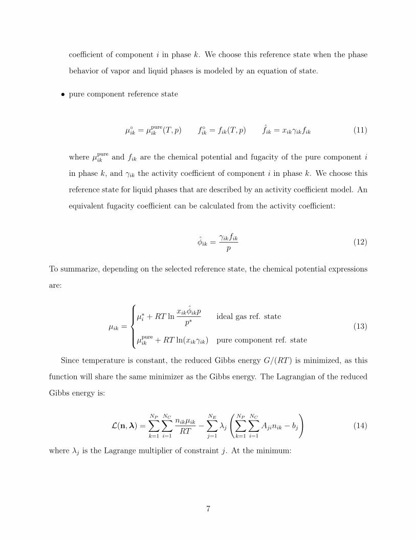
In this work we show how the modified RAND can be used to calculate multiphase

chemical equilibrium. We present the modified RAND method and implement it on ideal

and non-ideal vapor-liquid (VLE), liquid-liquid (LLE) and vapor-liquid-liquid equilibrium

(VLLE) of different reaction systems. Computations begin with the assumption of a single-

phase. Initialization of the modified RAND is performed by a nested-loop procedure, deter-

mining Lagrange multipliers and phase amounts in the inner loop, while updating fugacity

or activity coefficients in the outer loop.2 This is essentially a first-order successive substi-

tution step. If there is no convergence after three outer-loop iterations, we switch over to

the modified RAND, to accelerate calculations. Finally, stability analysis is performed to

check whether the current phase set is stable, and if not, to introduce an additional phase.

After the introduction of a new phase, the same successive substitution and modified RAND

steps are repeated until the obtained solution is proven stable by the stability analysis. The

algorithm is efficient and robust, without any incidents of divergence or failure for systems

and conditions tested.

Method

Gibbs energy minimization

Chemical and phase equilibrium at constant temperature and pressure is determined by min-

imizing the total Gibbs energy of the system. When NC components undergo NR chemical

reactions, they are not independent. Instead, there are NE = NC −NR independent entities

required to fully characterize the system and they are called elements. For NP phases, the

4

constrained minimization problem under the material balance and non-negativity constraints

is formulated as:

minnG(T, p,n) = min

nik

NP∑k=1

NC∑i=1

nikµik(T, p,nk)

s.t.NP∑k=1

NC∑i=1

Ajinik = bj, j = 1, ..., NE

nik ≥ 0, i = 1, ..., NC k = 1, ..., NP

(1)

where G is the Gibbs energy of the system, T the temperature, p the pressure, nik and µik the

mole numbers and chemical potential of component i in phase k, n and nk the component

abundance matrix (entries nik) and component abundance vector in phase k, Aji the number

of elements j in component i and bj the total mole numbers of element j.

The material balance in matrix-vector form is expressed in terms of the formula matrix

A and the element abundance vector b:

A

NP∑k=1

nk = b (2)

The element abundance vector is constant no matter how much the reactions progress.

Therefore, it is calculable from feed information:

b = AnF (3)

where nF is the components abundance vector of the single-phase feed. The material balance

refers to the total mole numbers of the elements in the system. Mole numbers of elements

in phase k are found from Bk:

Bk = Ank (4)

and different phases can be combined in the elements abundance matrix B:

5

B = An (5)

Linearizing Eq. 2 around the mole numbers estimates, we obtain:

A

NP∑k=1

(nk + ∆nk) = b (6)

or

A

NP∑k=1

∆nk = 0 (7)

This equation is valid only when mole numbers satisfy the material balance. Otherwise, we

have in general:

A

NP∑k=1

∆nk = ∆b =

0 material balance satisfied

b−∑NP

k=1Bk material balance not satisfied(8)

Chemical potentials are calculated by:

µik = µ◦ik +RT lnf̂ikf ◦ik

(9)

where µ◦ik and f ◦ik are the reference state chemical potential and reference state fugacity of

component i in phase k, f̂ik the fugacity of component i in phase k, and R the gas constant.

The reference states used in this work are two:

• ideal gas reference state

µ◦ik = µ∗i (T ) f ◦ik = p∗ f̂ik = xikφ̂ikp (10)

where µ∗i (T ) is the ideal gas chemical potential of component i, p∗ the unit pressure

(1 bar or 1 atm), xik the mole fraction of component i in phase k and φ̂ik the fugacity

6

coefficient of component i in phase k. We choose this reference state when the phase

behavior of vapor and liquid phases is modeled by an equation of state.

• pure component reference state

µ◦ik = µpureik (T, p) f ◦ik = fik(T, p) f̂ik = xikγikfik (11)

where µpureik and fik are the chemical potential and fugacity of the pure component i

in phase k, and γik the activity coefficient of component i in phase k. We choose this

reference state for liquid phases that are described by an activity coefficient model. An

equivalent fugacity coefficient can be calculated from the activity coefficient:

φ̂ik =γikfikp

(12)

To summarize, depending on the selected reference state, the chemical potential expressions

are:

µik =

µ∗i +RT ln

xikφ̂ikp

p∗ideal gas ref. state

µpureik +RT ln(xikγik) pure component ref. state

(13)

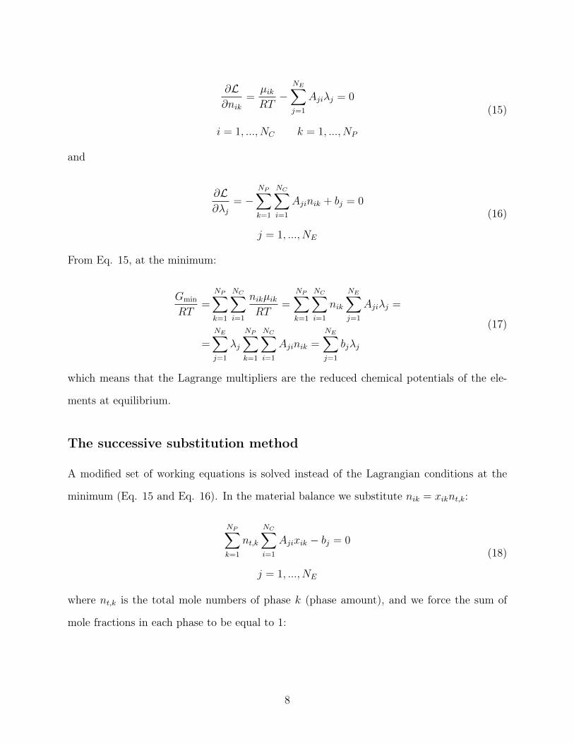
Since temperature is constant, the reduced Gibbs energy G/(RT ) is minimized, as this

function will share the same minimizer as the Gibbs energy. The Lagrangian of the reduced

Gibbs energy is:

L(n,λ) =

NP∑k=1

NC∑i=1

nikµik

RT−

NE∑j=1

λj

(NP∑k=1

NC∑i=1

Ajinik − bj

)(14)

where λj is the Lagrange multiplier of constraint j. At the minimum:

7

∂L∂nik

=µik

RT−

NE∑j=1

Ajiλj = 0

i = 1, ..., NC k = 1, ..., NP

(15)

and

∂L∂λj

= −NP∑k=1

NC∑i=1

Ajinik + bj = 0

j = 1, ..., NE

(16)

From Eq. 15, at the minimum:

Gmin

RT=

NP∑k=1

NC∑i=1

nikµik

RT=

NP∑k=1

NC∑i=1

nik

NE∑j=1

Ajiλj =

=

NE∑j=1

λj

NP∑k=1

NC∑i=1

Ajinik =

NE∑j=1

bjλj

(17)

which means that the Lagrange multipliers are the reduced chemical potentials of the ele-

ments at equilibrium.

The successive substitution method

A modified set of working equations is solved instead of the Lagrangian conditions at the

minimum (Eq. 15 and Eq. 16). In the material balance we substitute nik = xiknt,k:

NP∑k=1

nt,k

NC∑i=1

Ajixik − bj = 0

j = 1, ..., NE

(18)

where nt,k is the total mole numbers of phase k (phase amount), and we force the sum of

mole fractions in each phase to be equal to 1:

8

NC∑i=1

xik − 1 = 0

k = 1, ..., NP

(19)

From Eq. 15 we can express mole fractions as a function of the Lagrange multipliers. For

the ideal gas reference state:

lnxik =

NE∑j=1

Ajiλj −µ∗iRT− ln

φ̂ikp

p∗(20)

and for the pure component reference state:

lnxik =

NE∑j=1

Ajiλj −µpureik

RT− ln γik (21)

To determine the equilibrium solution, we need to solve Eq. 18 and Eq. 19 for NE Lagrange

multipliers and NP phase amounts, using Eq. 20 or Eq. 21. In a nested-loop, fugacity or

activity coefficients are assumed composition independent in the inner loop and updated in

the outer loop. From Eq. 20 or Eq. 21, composition independence results in:

∂xik∂λq

= Aqixik

q = 1, ..., NE

(22)

and

∂xik∂nt,q

= 0

q = 1, ..., NP

(23)

The system in the inner loop becomes:

A diag(∑NP

k=1 nk

)AT Ax

(Ax)T 0

∆λ

∆nt

= −

A∑NP

k=1 nk − b

xTeNC− eNP

(24)

9

where x is the mole fraction matrix with entries xik and eX is a vector of ones with dimensions

X × 1.

The modified RAND method

The RAND method, originally proposed by White et al. 5 , is only for ideal systems: vapor

phases with fugacity coefficients or liquid phases with activity coefficients equal to 1. We

present here its extension to the general case where the equilibrium phases are non-ideal.

Eq. 15 can be linearized around the mole numbers estimates:

µik

RT+

NC∑q=1

∂

∂nqk

( µik

RT

)∆nqk −

NE∑j=1

λjAji = 0

i = 1, ..., NC k = 1, ..., NP

(25)

Mole number derivatives of the chemical potentials are calculated by:

∂

∂nqk

( µik

RT

)=δiqnik

− 1

nt,k

+∂ ln φ̂ik

∂nqk

(26)

where δiq is the Kronecker delta. If an activity coefficient model is used for a liquid phase,

activity coefficient derivatives are equivalent (Eq. 12):

∂ ln γik∂nqk

=∂ ln φ̂ik

∂nqk

∀ q 6= i k = 1, ..., NP

(27)

The corrections to the mole numbers ∆nik must be isolated. According to the Gibbs-Duhem

equation, the matrix of the mole number derivatives of the chemical potentials in a specific

phase is singular:

NC∑i=1

nik∂µik

∂nqk

=

NC∑i=1

nik∂ ln φ̂ik

∂nqk

= 0

q = 1, ..., NC k = 1, ..., NP

(28)

10

and therefore not invertible. We define the following:

Miqk =δiqnik

+∂ ln φ̂ik

∂nqk

(29)

and

sk =

∑NC

i=1 ∆nik

nt,k

=∆nt,k

nt,k

=∆nt,k

eTNCnk

(30)

The matrix-vector form of Eq. 25 for phase k is:

µk

RT+ Mk∆nk − skeNC

−ATλ = 0

k = 1, ..., NP

(31)

Corrections for the component abundance vectors are given by:

∆nk = M−1k eNC

sk + M−1k

(ATλ− µk

RT

)k = 1, ..., NP

(32)

From Eq. 28 we obtain:

Mknk = eNC

k = 1, ..., NP

(33)

and by inverting matrix Mk:

nk = M−1k eNC

k = 1, ..., NP

(34)

Using Eq. 34, the correction vectors become:

∆nk = nksk + M−1k

(ATλ− µk

RT

)k = 1, ..., NP

(35)

11

There are two equations the correction vectors ∆nk must satisfy:

A

NP∑k=1

∆nk = ∆b (36)

and

eTNC∆nk = ∆nt,k

k = 1, ..., NP

(37)

Substitution of Eq. 35 in Eq. 36 results in:

A

NP∑k=1

nksk + A

NP∑k=1

M−1k ATλ−A

NP∑k=1

M−1k

µk

RT= ∆b (38)

or

(A

NP∑k=1

M−1k AT

)λ + Bs = A

NP∑k=1

M−1k

µk

RT+ ∆b (39)

Substitution of Eq. 35 in Eq. 37 results in:

eTNCnksk + eTNC

M−1k

(ATλ− µk

RT

)= ∆nt,k

k = 1, ..., NP

(40)

Matrix Mk is symmetric, because:

∂ ln φ̂ik

∂nqk

=∂ ln φ̂qk

∂nik

∀ q 6= i k = 1, ..., NP

(41)

therefore, taking the transpose of Eq. 34:

nTk = eTNC

M−1k

k = 1, ..., NP

(42)

12

From Eq. 30 and Eq. 42, we get in Eq. 40:

nTk

(ATλ− µk

RT

)= 0

k = 1, ..., NP

(43)

or

BTkλ =

nTkµk

RT

k = 1, ..., NP

(44)

Finally, the modified RAND method for non-ideal multiphase systems requires solving the

system of Eq. 39 and Eq. 44:

A∑NP

k=1M−1k AT B

BT 0

λs

=

A∑NP

k=1M−1k (µk/RT ) + ∆b

d

(45)

where:

dk =nTkµk

RT(46)

If the initial mole numbers estimate satisfies the material balance, the mole numbers at

every iteration will satisfy it as well. This is an important advantage of the RAND metod,

since the value of the Gibbs energy can be constantly monitored for the potential need

of corrective action. At every iteration, λ and s are determined, corrections to the mole

numbers are calculated by Eq. 35 and the mole numbers are updated as:

n(q+1)k = n

(q)k + α∆n

(q)k

k = 1, ..., NP

(47)

where q is the current iteration and α controls the step in case of objective function increase

or negative mole numbers. In Eq. 45, the value of ∆b can be set to 0, if the initial values

of mole numbers satisfy the material balance (Eq. 8). However, in our implementation we

13

preserve it in the general form ∆b = b−∑NP

k=1Bk, in order to mitigate the effect of round-off

errors.

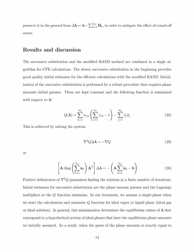
Results and discussion

The successive substitution and the modified RAND method are combined in a single al-

gorithm for CPE calculations. The slower successive substitution in the beginning provides

good quality initial estimates for the efficient calculations with the modified RAND. Initial-

ization of the successive substitution is performed by a robust procedure that requires phase

amounts initial guesses. These are kept constant and the following function is minimized

with respect to λ:

Q(λ) =

NP∑k=1

nt,k

(NC∑i=1

xik − 1

)−

NE∑j=1

λjbj (48)

This is achieved by solving the system:

∇2Q∆λ = −∇Q (49)

or

[A diag

(NP∑k=1

nk

)AT

]∆λ = −

(A

NP∑k=1

nk − b

)(50)

Positive definiteness of ∇2Q guarantees finding the solution in a finite number of iterations.

Initial estimates for successive substitution are the phase amount guesses and the Lagrange

multipliers at the Q function minimum. In our treatment, we assume a single-phase when

we start the calculations and minimize Q function for ideal vapor or liquid phase (ideal gas

or ideal solution). In general, this minimization determines the equilibrium values of λ that

correspond to a hypothetical system of ideal phases that have the equilibrium phase amounts

we initially assumed. As a result, when the guess of the phase amounts is exactly equal to

14

their actual equilibrium values and the phases are ideal, Q function minimization determines

the final solution of Eq. 24.

We allow successive substitution to run for up to three iterations. If there is no conver-

gence, the modified RAND method is ultimately employed until full convergence. Finally,

stability analysis is performed as mentioned in Michelsen 17 , to judge if an additional phase

should be considered. The equations are solved again for the new phase set, however, Q

function minimization is now skipped. This summarizes the combined algorithm. An alter-

native algorithm uses only the successive substitution method with the same initialization

and stability as mentioned above. This is the successive substitution algorithm. The main

steps of the two algorithms can be seen in Figure 1. The error for successive substitution at

iteration q is calculated by:

error(q) =

√√√√ NE∑j=1

[λ(q)j − λ

(q−1)j

]2+

NP∑k=1

[n(q)t,k − n

(q−1)t,k

]2(51)

and for the modified RAND by:

error(q) =

√√√√ NP∑k=1

NC∑i=1

[n(q)ik − n

(q−1)ik

]2(52)

Convergence to the solution is assumed when the error is less than 10−10. Table 1 presents

the numbering of components and elements for all the systems examined. Equilibrium results

are reported, along with convergence behavior, where the combined algorithm is expected

to perform rapid calculations compared with the slower successive substitution.

Table 1: Component and element numbering for the systems in this work.

System 1 2 3 4 5

Acetic acid/1-butanol Component Acetic acid 1-Butanol Water Butyl acetateesterification Element C2H2O C4H10O H2O

Propene Component Propene Water 2-Propanolhydration Element C3H6 H2O

TAME synthesis Component 2-Methyl-1-butene 2-Methyl-2-butene Methanol TAME n-Pentane1 reaction Element C2.5H5 C2.5H5 CH4O C5H12

2 reactions Element C5H10 CH4O C5H12

15

Set T , p, nF , NP = 1and guess nt

Find λ initial estimatesfrom the nt guess

Solve equationswith Newton’s method

All phasesideal? Update γ or φ̂NP = NP + 1

Stable? Converged?

Get λ, nt and xk

yes no

yes no

yes

no

(a)

Set T , p, nF , NP = 1and guess nt

Find λ initial estimatesfrom the nt guess

Successive substitutionfor up to 3 iterations

Converged?

RAND

NP = NP + 1

Stable?

Get λ, nt and xk

yes

no

yes

no

(b)

Figure 1: Main steps for the successive substitution (a) and the combined algorithm (b).

Esterification of acetic acid with 1-butanol

Wasylkiewicz and Ung 18 studied the LLE in the esterification of acetic acid with 1-butanol

to water and butyl acetate:

C2H4O2 + C4H10O⇀↽ H2O + C6H12O2 (53)

The number of elements isNE = NC−NR = 4−1 = 3. The formula matrix and stoichiometric

matrix of the system are given by:

A =

1 0 0 1

0 1 0 1

1 0 1 0

N =

[−1 −1 1 1

]T(54)

The vapor phase is considered ideal and liquid phases are described by the UNIQUAC

activity coefficient model.19 The chemical equilibrium constant was taken from Wasylkiewicz

and Ung 18 , vapor pressure expressions and parameters for the UNIQUAC model were taken

from Okasinski and Doherty 20 . Calculations for LLE are compared with Bonilla-Petriciolet

16

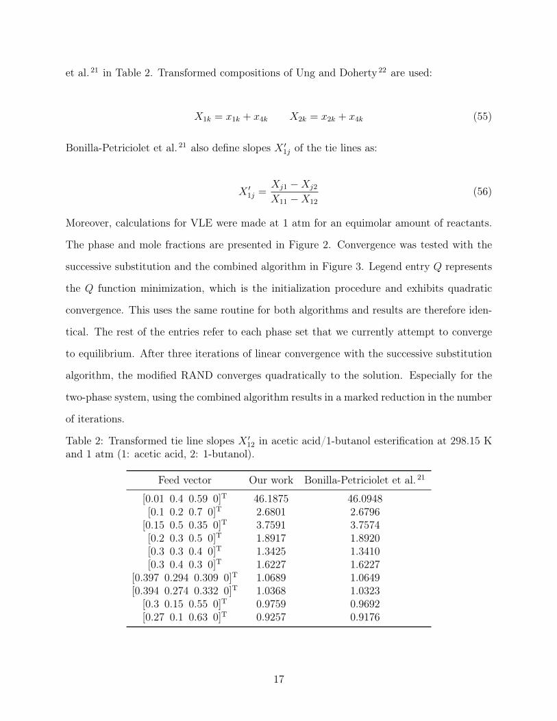
et al. 21 in Table 2. Transformed compositions of Ung and Doherty 22 are used:

X1k = x1k + x4k X2k = x2k + x4k (55)

Bonilla-Petriciolet et al. 21 also define slopes X ′1j of the tie lines as:

X ′1j =Xj1 −Xj2

X11 −X12

(56)

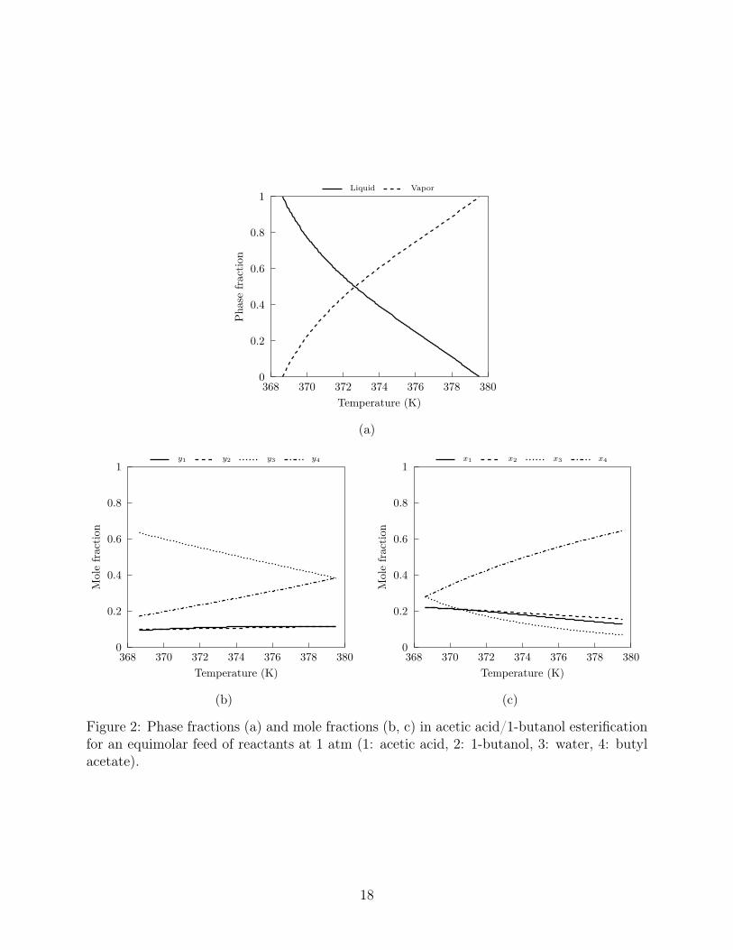
Moreover, calculations for VLE were made at 1 atm for an equimolar amount of reactants.

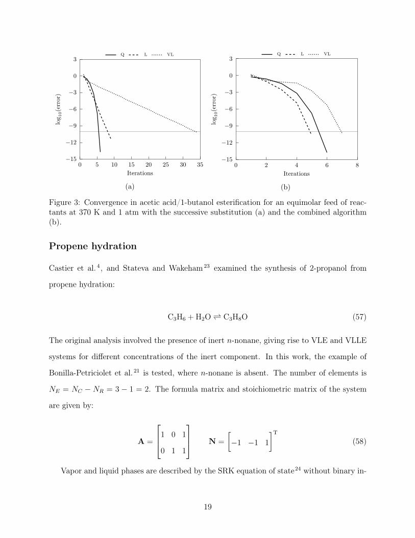
The phase and mole fractions are presented in Figure 2. Convergence was tested with the

successive substitution and the combined algorithm in Figure 3. Legend entry Q represents

the Q function minimization, which is the initialization procedure and exhibits quadratic

convergence. This uses the same routine for both algorithms and results are therefore iden-

tical. The rest of the entries refer to each phase set that we currently attempt to converge

to equilibrium. After three iterations of linear convergence with the successive substitution

algorithm, the modified RAND converges quadratically to the solution. Especially for the

two-phase system, using the combined algorithm results in a marked reduction in the number

of iterations.

Table 2: Transformed tie line slopes X ′12 in acetic acid/1-butanol esterification at 298.15 Kand 1 atm (1: acetic acid, 2: 1-butanol).

Feed vector Our work Bonilla-Petriciolet et al. 21

[0.01 0.4 0.59 0]T 46.1875 46.0948[0.1 0.2 0.7 0]T 2.6801 2.6796

[0.15 0.5 0.35 0]T 3.7591 3.7574[0.2 0.3 0.5 0]T 1.8917 1.8920[0.3 0.3 0.4 0]T 1.3425 1.3410[0.3 0.4 0.3 0]T 1.6227 1.6227

[0.397 0.294 0.309 0]T 1.0689 1.0649[0.394 0.274 0.332 0]T 1.0368 1.0323

[0.3 0.15 0.55 0]T 0.9759 0.9692[0.27 0.1 0.63 0]T 0.9257 0.9176

17

368 370 372 374 376 378 3800

0.2

0.4

0.6

0.8

1

Temperature (K)

Phas

efra

ctio

n

Liquid Vapor

(a)

368 370 372 374 376 378 3800

0.2

0.4

0.6

0.8

1

Temperature (K)

Mol

efra

ctio

n

y1 y2 y3 y4

(b)

368 370 372 374 376 378 3800

0.2

0.4

0.6

0.8

1

Temperature (K)

Mol

efra

ctio

n

x1 x2 x3 x4

(c)

Figure 2: Phase fractions (a) and mole fractions (b, c) in acetic acid/1-butanol esterificationfor an equimolar feed of reactants at 1 atm (1: acetic acid, 2: 1-butanol, 3: water, 4: butylacetate).

18

0 5 10 15 20 25 30 35−15

−12

−9

−6

−3

0

3

Iterations

log 1

0(er

ror)

Q L VL

(a)

0 2 4 6 8−15

−12

−9

−6

−3

0

3

Iterations

log 1

0(er

ror)

Q L VL

(b)

Figure 3: Convergence in acetic acid/1-butanol esterification for an equimolar feed of reac-tants at 370 K and 1 atm with the successive substitution (a) and the combined algorithm(b).

Propene hydration

Castier et al. 4 , and Stateva and Wakeham 23 examined the synthesis of 2-propanol from

propene hydration:

C3H6 + H2O⇀↽ C3H8O (57)

The original analysis involved the presence of inert n-nonane, giving rise to VLE and VLLE

systems for different concentrations of the inert component. In this work, the example of

Bonilla-Petriciolet et al. 21 is tested, where n-nonane is absent. The number of elements is

NE = NC − NR = 3 − 1 = 2. The formula matrix and stoichiometric matrix of the system

are given by:

A =

1 0 1

0 1 1

N =

[−1 −1 1

]T(58)

Vapor and liquid phases are described by the SRK equation of state24 without binary in-

19

teraction parameters. The chemical equilibrium constant was taken from Bonilla-Petriciolet

et al. 21 and was considered temperature independent. The calculation results using a tem-

perature dependent equilibrium constant are provided in the Supporting Information. Cal-

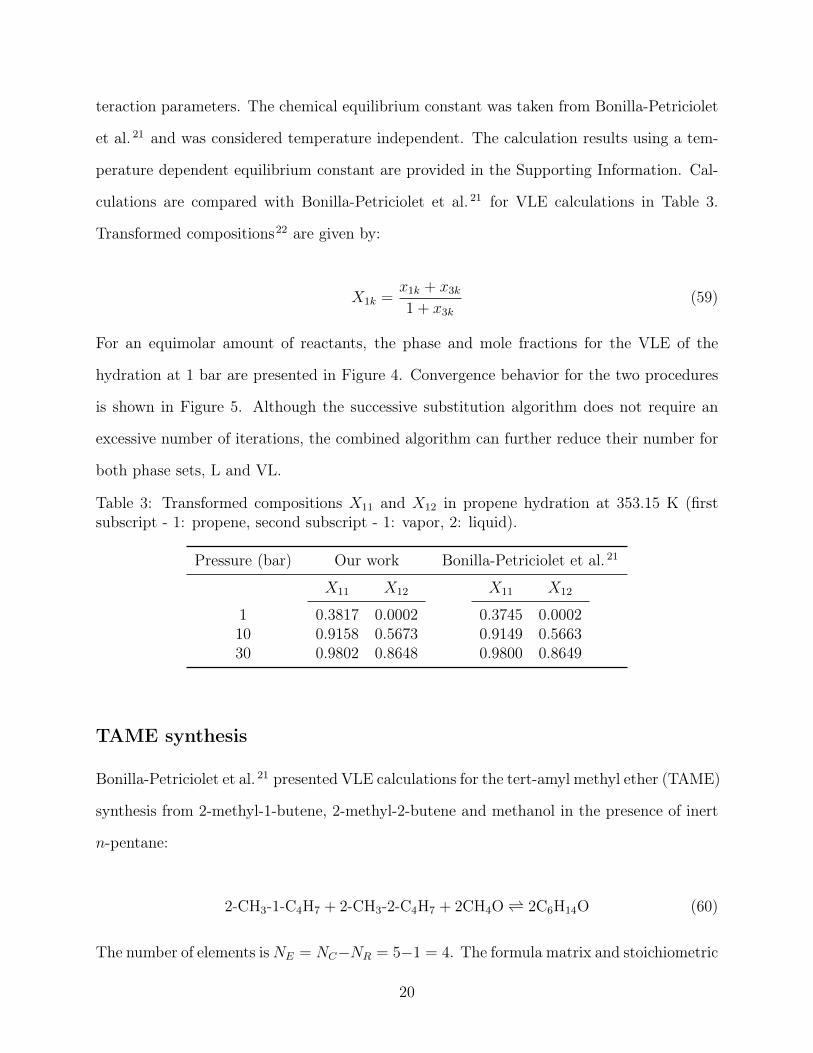
culations are compared with Bonilla-Petriciolet et al. 21 for VLE calculations in Table 3.

Transformed compositions22 are given by:

X1k =x1k + x3k1 + x3k

(59)

For an equimolar amount of reactants, the phase and mole fractions for the VLE of the

hydration at 1 bar are presented in Figure 4. Convergence behavior for the two procedures

is shown in Figure 5. Although the successive substitution algorithm does not require an

excessive number of iterations, the combined algorithm can further reduce their number for

both phase sets, L and VL.

Table 3: Transformed compositions X11 and X12 in propene hydration at 353.15 K (firstsubscript - 1: propene, second subscript - 1: vapor, 2: liquid).

Pressure (bar) Our work Bonilla-Petriciolet et al. 21

11030

X11 X12

0.3817 0.00020.9158 0.56730.9802 0.8648

X11 X12

0.3745 0.00020.9149 0.56630.9800 0.8649

TAME synthesis

Bonilla-Petriciolet et al. 21 presented VLE calculations for the tert-amyl methyl ether (TAME)

synthesis from 2-methyl-1-butene, 2-methyl-2-butene and methanol in the presence of inert

n-pentane:

2-CH3-1-C4H7 + 2-CH3-2-C4H7 + 2CH4O⇀↽ 2C6H14O (60)

The number of elements isNE = NC−NR = 5−1 = 4. The formula matrix and stoichiometric

20

330 333 336 339 342 345 3480

0.2

0.4

0.6

0.8

1

Temperature (K)

Phas

efra

ctio

n

Liquid Vapor

(a)

330 333 336 339 342 345 3480

0.2

0.4

0.6

0.8

1

Temperature (K)

Mol

efra

ctio

n

y1 y2 y3

(b)

330 333 336 339 342 345 3480

0.2

0.4

0.6

0.8

1

Temperature (K)

Mol

efra

ctio

n

x1 x2 x3

(c)

Figure 4: Phase fractions (a) and mole fractions (b, c) in propene hydration for an equimolarfeed of reactants at 1 bar (1: propene, 2: water, 3: 2-propanol).

21

0 2 4 6 8 10−15

−12

−9

−6

−3

0

3

Iterations

log 1

0(er

ror)

Q L VL

(a)

0 2 4 6 8 10−15

−12

−9

−6

−3

0

3

Iterations

log 1

0(er

ror)

Q L VL

(b)

Figure 5: Convergence in propene hydration for an equimolar feed of reactants at 345 K and1 bar with the successive substitution (a) and the combined algorithm (b).

matrix of the system are given by:

A =

2 0 0 1 0

0 2 0 1 0

0 0 1 1 0

0 0 0 0 1

N =

[−1 −1 −2 2 0

]T(61)

The vapor phase is considered ideal and the liquid phase is described by the Wilson

activity coefficient model.25 The chemical equilibrium constant was taken from Bonilla-

Petriciolet et al. 21 , vapor pressure expressions and parameters for the Wilson model were

taken from Chen et al. 26 . Calculations are compared with Bonilla-Petriciolet et al. 21 for the

VLE of the system in Table 4. Transformed compositions of Ung and Doherty 22 are used:

X1k =x1k + 0.5x4k

1 + x4kX2k =

x2k + 0.5x4k1 + x4k

X3k =x3k + x4k1 + x4k

(62)

where tie line slopes are defined by Eq. 56.

Chen et al. 26 study the kinetics in reactive distillation of TAME. In their analysis, two

reactions take place in the column:

22

Table 4: Transformed tie lines slopes X ′12 and X ′13 in TAME synthesis for the single-reactionsystem at 335 K and 1.52 bar (1: 2-methyl-1-butene, 2: 2-methyl-2-butene, 3: methanol).

Feed vector Our work Bonilla-Petriciolet et al. 21

[0.3 0.15 0.55 0 0]T

[0.32 0.2 0.48 0 0]T

[0.354 0.183 0.463 0 0]T

[0.2 0.07 0.73 0 0]T

[0.15 0.02 0.83 0 0]T

[0.27 0.3 0.43 0 0]T

[0.2 0.35 0.45 0 0]T

[0.1 0.35 0.55 0 0]T

[0.05 0.3 0.65 0 0]T

[0.025 0.3 0.675 0 0]T

[0.15 0.02 0.8 0 0.03]T

[0.1 0.1 0.6 0 0.2]T

[0.05 0.05 0.85 0 0.05]T

[0.1 0.15 0.7 0 0.05]T

[0.15 0.15 0.6 0 0.1]T

[0.07 0.17 0.64 0 0.12]T

X ′12 X ′13

-0.2083 --0.2813 --0.2869 --0.0079 -0.0063 -0.8050 --3.6530 --8.4680 --157.8824 -334.3359 -0.0098 -1.24280.9404 -5.83880.8065 -6.25046.0678 -13.54630.8456 -4.04667.9465 -18.0942

X ′12 X ′13

-0.2072 --0.2800 --0.2856 --0.0076 -0.0064 -0.8089 --3.6767 --8.5301 --162.6184 -327.5080 -0.0099 -1.24280.9406 -5.83400.8069 -6.24386.0243 -13.44450.8465 -4.03967.9130 -18.0152

2-CH3-1-C4H7 + CH4O⇀↽ C6H14O (63)

2-CH3-2-C4H7 + CH4O⇀↽ C6H14O (64)

creating a different reaction system. The number of elements is now NE = NC − NR =

5− 2 = 3. The formula matrix and stoichiometric matrix of the system are given by:

A =

1 1 0 1 0

0 0 1 1 0

0 0 0 0 1

N =

−1 0 −1 1 0

0 −1 −1 1 0

T

(65)

The chemical equilibrium constants for the two reactions were taken from Chen et al. 26 .

Although Bonilla-Petriciolet et al. 21 combined the two reactions by addition (Eq. 60), the

23

chemical equilibrium constant they use corresponds to the reaction of Eq. 63 according to

Chen et al. 26 . For a stoichiometric feed of reactants and methanol/n-pentane ratio 2:1, the

phase and mole fractions for the two-reaction VLE calculations at 1.52 bar are presented in

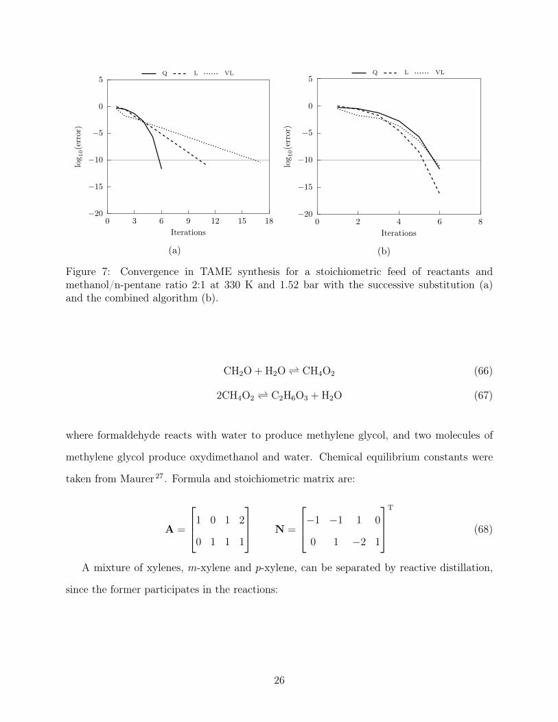
Figure 6. Convergence for the 2-reaction TAME synthesis is shown in Figure 7. It is evident

that the successive substitution algorithm requires two to three times more iterations to

fully converge, in comparison with the combined algorithm which performs much faster

calculations.

Comparison of convergence with previously reported systems

Several systems were tested in previous work using only the successive substitution al-

gorithm.2 Components and elements of the additional systems are presented in Table 5.

Convergence behavior will be examined with the combined algorithm and compared with

successive substitution results.

Table 5: Component and element numbering for the systems tested in previous work.

System 1 2 3 4 5 6 7

Formaldehyde/ Component Formaldehyde Water Methylene glycol Oxydimethanolwater Element CH2O H2O

Xylene Component Di-tert-butylbenzene m-Xylene tert-Butyl-m-xylene tert-Butylbenzene Benzene p-Xyleneseparation Element C6H6 C4H8 C8H10 C8H10

Acetic acid/ethanol Component Acetic acid Ethanol Water Ethyl acetateesterification Element C2H2O C2H6O H2O

MTBE Component Isobutene Methanol n-Butane MTBEsynthesis Element C4H8 CH4O C4H10

Cyclohexane Component Benzene Hydrogen Cyclohexanesynthesis Element C6H6 H2

Methanol Component Carbon monoxide Carbon dioxide Hydrogen Water Methanol Methane Octadecanesynthesis Element CO O H2 CH4 C18H38

Formaldehyde/water based system and xylene separation

Formaldehyde dimerization is studied based on the following reactions:

24

328 329 330 331 332 333 3340

0.2

0.4

0.6

0.8

1

Temperature (K)

Phas

efra

ctio

n

Liquid Vapor

(a)

328 329 330 331 332 333 3340

0.2

0.4

0.6

0.8

1

Temperature (K)

Mol

efra

ctio

n

y1 y2 y3 y4 y5

(b)

328 329 330 331 332 333 3340

0.2

0.4

0.6

0.8

1

Temperature (K)

Mol

efra

ctio

n

x1 x2 x3 x4 x5

(c)

Figure 6: Phase fractions (a) and vapor/liquid phase mole fractions (b, c) in TAME synthesisat 1.52 bar for a stoichiometric feed of reactants and methanol/n-pentane ratio 2:1 (1: 2-methyl-1-butene, 2: 2-methyl-2-butene, 3: methanol, 4: TAME, 5: n-pentane).

25

0 3 6 9 12 15 18−20

−15

−10

−5

0

5

Iterations

log 1

0(er

ror)

Q L VL

(a)

0 2 4 6 8−20

−15

−10

−5

0

5

Iterations

log 1

0(er

ror)

Q L VL

(b)

Figure 7: Convergence in TAME synthesis for a stoichiometric feed of reactants andmethanol/n-pentane ratio 2:1 at 330 K and 1.52 bar with the successive substitution (a)and the combined algorithm (b).

CH2O + H2O⇀↽ CH4O2 (66)

2CH4O2 ⇀↽ C2H6O3 + H2O (67)

where formaldehyde reacts with water to produce methylene glycol, and two molecules of

methylene glycol produce oxydimethanol and water. Chemical equilibrium constants were

taken from Maurer 27 . Formula and stoichiometric matrix are:

A =

1 0 1 2

0 1 1 1

N =

−1 −1 1 0

0 1 −2 1

T

(68)

A mixture of xylenes, m-xylene and p-xylene, can be separated by reactive distillation,

since the former participates in the reactions:

26

C14H22 +m-C8H10 ⇀↽ C12H18 + C10H14 (69)

C10H14 +m-C8H10 ⇀↽ C12H18 + C6H6 (70)

where di-tert-butylbenzene reacts withm-xylene to give tert-butyl-m-xylene and tert-butylbenzene,

while tert-butylbenzene reacts with m-xylene to produce tert-butyl-m-xylene and benzene

(p-xylene is an inert). Chemical equilibrium constants were taken from Saito et al. 28 . For-

mula matrix and stoichiometric matrix are:

A =

1 0 0 1 1 0

2 0 1 1 0 0

0 1 1 0 0 0

0 0 0 0 0 1

N =

−1 −1 1 1 0 0

0 −1 1 −1 1 0

T

(71)

The vapor and the liquid phase of both systems were considered ideal. As a result,

there is no need for an outer loop to update activity coefficients. This allows the successive

substitution algorithm to attain quadratic convergence rate and no direct comparison was

made with the combined algorithm.

Esterification of acetic acid with ethanol

Esterification of acetic acid with ethanol to water and ethyl acetate is given by the reaction:

C2H4O2 + C2H6O⇀↽ C4H8O2 + H2O (72)

The vapor phase is considered ideal and the liquid phase is described by the UNIQUAC

activity coefficient model.19 The chemical equilibrium constant and parameters for the phase

equilibrium model were reported in Xiao et al. 29 . Formula matrix and stoichiometric matrix

are:

27

A =

1 0 0 1

0 1 0 1

1 0 1 0

N =

[−1 −1 1 1

]T(73)

In Figure 8 convergence of the two reported procedures is presented. When successive

substitution is employed (successive substitution algorithm or the first steps of the combined

algorithm), only the outer loop iterations are shown. For this system we begin with the

assumption of a single ideal vapor phase. Moreover, the total mole numbers do not change

due to the reaction, which means that the phase amount is known at the supposed single-

phase equilibrium. Therefore, minimization of function Q produces the actual equilibrium

concentrations of the single ideal vapor phase and successive substitution is not needed. For

the two-phase system, we obtain the solution in 7 iterations with the combined algorithm,

compared to 44 with just successive substitution.

0 8 16 24 32 40 48−16

−12

−8

−4

0

4

Iterations

log 1

0(er

ror)

Q V VL

(a)

0 2 4 6 8 10−16

−12

−8

−4

0

4

Iterations

log 1

0(er

ror)

Q V VL

(b)

Figure 8: Convergence in acetic acid/ethanol esterification for an equimolar feed of reactantsat 355 K and 1 atm with the successive substitution (a) and the combined algorithm (b).

MTBE synthesis

MTBE is synthesized from a mixture of isobutene and methanol:

28

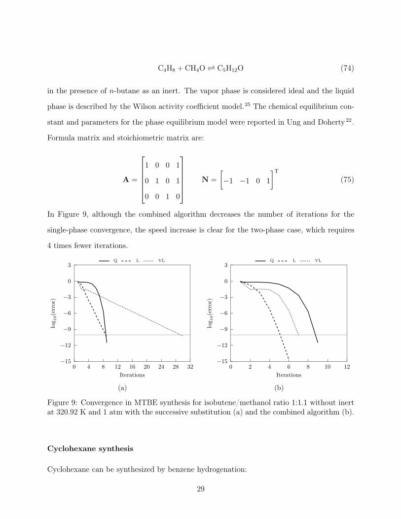
C4H8 + CH4O⇀↽ C5H12O (74)

in the presence of n-butane as an inert. The vapor phase is considered ideal and the liquid

phase is described by the Wilson activity coefficient model.25 The chemical equilibrium con-

stant and parameters for the phase equilibrium model were reported in Ung and Doherty 22 .

Formula matrix and stoichiometric matrix are:

A =

1 0 0 1

0 1 0 1

0 0 1 0

N =

[−1 −1 0 1

]T(75)

In Figure 9, although the combined algorithm decreases the number of iterations for the

single-phase convergence, the speed increase is clear for the two-phase case, which requires

4 times fewer iterations.

0 4 8 12 16 20 24 28 32−15

−12

−9

−6

−3

0

3

Iterations

log 1

0(er

ror)

Q L VL

(a)

0 2 4 6 8 10 12−15

−12

−9

−6

−3

0

3

Iterations

log 1

0(er

ror)

Q L VL

(b)

Figure 9: Convergence in MTBE synthesis for isobutene/methanol ratio 1:1.1 without inertat 320.92 K and 1 atm with the successive substitution (a) and the combined algorithm (b).

Cyclohexane synthesis

Cyclohexane can be synthesized by benzene hydrogenation:

29

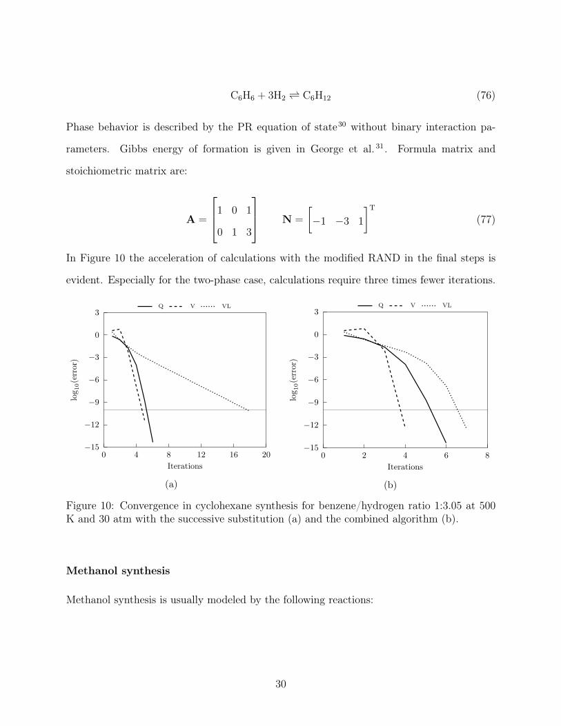
C6H6 + 3H2 ⇀↽ C6H12 (76)

Phase behavior is described by the PR equation of state30 without binary interaction pa-

rameters. Gibbs energy of formation is given in George et al. 31 . Formula matrix and

stoichiometric matrix are:

A =

1 0 1

0 1 3

N =

[−1 −3 1

]T(77)

In Figure 10 the acceleration of calculations with the modified RAND in the final steps is

evident. Especially for the two-phase case, calculations require three times fewer iterations.

0 4 8 12 16 20−15

−12

−9

−6

−3

0

3

Iterations

log 1

0(er

ror)

Q V VL

(a)

0 2 4 6 8−15

−12

−9

−6

−3

0

3

Iterations

log 1

0(er

ror)

Q V VL

(b)

Figure 10: Convergence in cyclohexane synthesis for benzene/hydrogen ratio 1:3.05 at 500K and 30 atm with the successive substitution (a) and the combined algorithm (b).

Methanol synthesis

Methanol synthesis is usually modeled by the following reactions:

30

CO + 2H2 ⇀↽ CH4O (78)

CO2 + H2 ⇀↽ CO + H2O (79)

with methane and n-octadecane included in the system as inerts. Phase behavior is described

by the SRK equation of state24 with binary interaction parameters reported by Castier

et al. 4 . Reference state chemical potentials at 1 bar are given in Phoenix and Heidemann 32 .

Formula matrix and stoichiometric matrix are:

A =

1 1 0 0 1 0 0

0 1 0 1 0 0 0

0 0 1 1 2 0 0

0 0 0 0 0 1 0

0 0 0 0 0 0 1

N =

−1 0 −2 0 1 0 0

1 −1 −1 1 0 0 0

T

(80)

Convergence of the three-phase methanol synthesis is shown in Figure 11. The first phase set,

a single vapor phase, requires 54 outer loop iterations with successive substitution. When

the modified RAND is employed after three successive substitution iterations, we need only

four additional iterations for full convergence. For the subsequent phase sets, VL and VLL,

the total number of iterations does not exceed eight, while using only successive substitution,

the minimum number of outer loop iterations is 22.

Conclusions

An efficient and robust algorithm combined of two non-stoichiometric methods is proposed

for non-ideal multiphase equilibrium of multicomponent reaction systems. Calculations begin

with the assumption of a single phase. A nested-loop procedure with successive substitution

is used during the first steps and for final convergence calculations are performed by the

31

0 8 16 24 32 40 48 56−16

−12

−8

−4

0

4

Iterations

log 1

0(er

ror)

Q V VL VLL

(a)

0 2 4 6 8 10 12−16

−12

−8

−4

0

4

Iterations

log 1

0(er

ror)

Q V VL VLL

(b)

Figure 11: Convergence in methanol synthesis at 473.15 K and 101.3 bar with the successivesubstitution (a) and the combined algorithm (b).

modified RAND method. Successive substitution provides good quality initial estimates for

modified RAND and stability analysis allows the sequential addition of the required number

of phases at equilibrium. The convergence rate is linear in the beginning and quadratic in

the final steps, due to the change of the procedure. No failure of convergence was observed

for a number of systems examined, regardless of the thermodynamic model that described

the phase behavior.

Supporting information

The current calculations in the cyclohexane synthesis were based on a temperature inde-

pendent chemical equilibrium constant. We have also examined the effect of temperature

dependence concerning chemical equilibrium. This information is available free of charge via

the Internet at http://pubs.acs.org/.

Acknowledgement

The authors thank Prof. Michael L. Michelsen for his insightful comments and suggestions.

32

References

(1) Smith, W. R.; Missen, R. W. Chemical Reaction Equilibrium Analysis: Theory and

Algorithms ; Wiley: New York, United States of America, 1982.

(2) Tsanas, C.; Stenby, E. H.; Yan, W. Calculation of Simultaneous Chemical and Phase

Equilibrium by the Method of Lagrange Multipliers. Chemical Engineering Science

2017, 174, 112–126.

(3) Michelsen, M. L.; Mollerup, J. M. Thermodynamic Models: Fundamentals & Compu-

tational Aspects, 2nd ed.; Tie-Line Publications: Holte, Denmark, 2007.

(4) Castier, M.; Rasmussen, P.; Fredenslund, A. Calculation of simultaneous chemical and

phase equilibria in nonideal systems. Chemical Engineering Science 1989, 44, 237–248.

(5) White, W. B.; Johnson, S. M.; Dantzig, G. B. Chemical Equilibrium in Complex Mix-

tures. The Journal of Chemical Physics 1958, 28, 751–755.

(6) Brinkley, S. R., Jr Calculation of the Equilibrium Composition of Systems of Many

Constituents. The Journal of Chemical Physics 1947, 15, 107–110.

(7) Huff, V. N.; Gordon, S.; Morrell, V. E. General method and thermodynamic tables

for computation of equilibrium composition and temperature of chemical reactions.

National Advisory Committee for Aeronautics 1951, NACA Technical Report 1037,

829–885.

(8) Gautam, R.; Seider, W. D. Computation of phase and chemical equilibrium: Part I.

Local and constrained minima in Gibbs free energy. AIChE Journal 1979, 25, 991–999.

(9) Gautam, R.; Seider, W. D. Computation of phase and chemical equilibrium: Part II.

Phase-splitting. AIChE Journal 1979, 25, 999–1006.

(10) Gautam, R.; Seider, W. D. Computation of phase and chemical equilibrium: Part III.

Electrolytic solutions. AIChE Journal 1979, 25, 1006–1015.

33

(11) White, C. W., III; Seider, W. D. Computation of phase and chemical equilibrium: Part

IV. Approach to chemical equilibrium. AIChE Journal 1981, 27, 466–471.

(12) Venkatraman, A.; Lake, L. W.; Johns, R. T. Gibbs Free Energy Minimization for

Prediction of Solubility of Acid Gases in Water. Industrial & Egineering Chemistry

Research 2014, 53, 6157–6168.

(13) Venkatraman, A.; Lake, L. W.; Johns, R. T. Modelling the impact of geochemical

reactions on hydrocarbon phase behavior during CO2 gas injection for enhanced oil

recovery. Fluid Phase Equilibria 2015, 402, 56–68.

(14) Voňka, P.; Leitner, J. Calculation of chemical equilibria in heterogeneous multicompo-

nent systems. Calphad 1995, 19, 25–36.

(15) Greiner, H. An efficient implementation of Newton’s method for complex nonideal chem-

ical equilibria. Computers & Chemical Engineering 1991, 15, 115–123.

(16) Paterson, D.; Michelsen, M. L.; Stenby, E. H.; Yan, W. New Formulations for Isothermal

Multiphase Flash. 2017; Submitted under the title “RAND-Based Formulations for

Isothermal Multiphase Flash” to Society of Petroleum Engineers Journal (accepted).

(17) Michelsen, M. L. The isothermal flash problem. Part I. Stability. Fluid Phase Equilibria

1982, 9, 1–19.

(18) Wasylkiewicz, S. K.; Ung, S. Global phase stability analysis for heterogeneous reac-

tive mixtures and calculation of reactive liquid-liquid and vapor-liquid-liquid equilibria.

Fluid Phase Equilibria 2000, 175, 253–272.

(19) Abrams, D. S.; Prausnitz, J. M. Statistical Thermodynamics of Liquid Mixtures: A

New Expression for the Excess Gibbs Energy of Partly or Completely Miscible Systems.

AIChE Journal 1975, 21, 116–128.

34

(20) Okasinski, M. J.; Doherty, M. F. Prediction of heterogeneous reactive azeotropes in

esterification systems. Chemical Engineering Science 2000, 55, 5263–5271.

(21) Bonilla-Petriciolet, A.; Bravo-Sánchez, U. I.; Castillo-Borja, F.; Frausto-Hernández, S.;

Segovia-Hernández, J. G. Gibbs Energy Minimization Using Simulated Annealing for

Two-phase Equilibrium Calculations in Reactive Systems. Chemical and Biochemical

Engineering Quarterly 2008, 22, 285–298.

(22) Ung, S.; Doherty, M. F. Vapor-liquid phase equilibrium in systems with multiple chem-

ical reactions. Chemical Engineering Science 1995, 50, 23–48.

(23) Stateva, R. P.; Wakeham, W. A. Phase Equilibrium Calculations for Chemically Re-

acting Systems. Industrial & Engineering Chemistry Research 1997, 36, 5474–5482.

(24) Soave, G. Equilibrium constants from a modified Redlich-Kwong equation of state.

Chemical Engineering Science 1972, 27, 1197–1203.

(25) Wilson, G. M. Vapor-Liquid Equilibrium. XI. A New Expression for the Excess Free

Energy of Mixing. Journal of the American Chemical Society 1964, 86, 127–130.

(26) Chen, F.; Huss, R. S.; Doherty, M. F.; Malone, M. F. Multiple steady states in reactive

distillation: kinetic effects. Computers & Chemical Engineering 2002, 26, 81–93.

(27) Maurer, G. Vapor-Liquid Equilibrium of Formaldehyde-and Water-Containing Multi-

component Mixtures. AIChE Journal 1986, 32, 932–948.

(28) Saito, S.; Michishita, T.; Maeda, S. Separation of meta- and para-xylene mixture by

distillation accompanied by chemical reactions. Journal of Chemical Engineering of

Japan 1971, 4, 37–43.

(29) Xiao, W.-d.; Zhu, K.-h.; Yuan, W.-k.; Chien, H. H.-y. An algorithm for simultaneous

chemical and phase equilibrium calculation. AIChE Journal 1989, 35, 1813–1820.

35

(30) Peng, D.-Y.; Robinson, D. B. A New Two-Constant Equation of State. Industrial &

Engineering Chemistry Fundamentals 1976, 15, 59–64.

(31) George, B.; Brown, L. P.; Farmer, C. H.; Buthod, P.; Manning, F. S. Computation of

Multicomponent, Multiphase Equilibrium. Industrial & Engineering Chemistry Process

Design and Development 1976, 15, 372–377.

(32) Phoenix, A. V.; Heidemann, R. A. A non-ideal multiphase chemical equilibrium algo-

rithm. Fluid Phase Equilibria 1998, 150–151, 255–265.

Table of Contents (TOC) Graphic

Set T , p, feed Initializationusing Q-function

Successivesubstitution

Modified RANDfor quadraticconvergence

Add a phase

Stabilityanalysis

Mutliphase chemicalequilibrium solution

stable

unstable

A + B C

Vapor

Liquid

36