1

NTNU Norwegian University of Science and Technology

Calculation of Natural Gas Mixture Phase Behavior at Low Temperature

Project Work of Subject

KP 8108 Advanced Thermodynamics

Student : Rahmat Nur Adi Wijaya

: Longman Zhang

Table of Contents Introduction ..................................................................................................................................... 3

1 Thermodynamics on Equilibrium Phase ................................................................................. 3

1.1 Phase Equilibria................................................................................................................ 3

1.2 Fugacity and Fugacity Coefficient ................................................................................... 5

1.3 Calculation of Fugacity Coefficient ................................................................................. 7

2 Phase Equilibrium by Equation of State ................................................................................. 9

2.1 Cubic Equation of State.................................................................................................... 9

2.2 Mixing Rules .................................................................................................................. 10

2.3 Application of EOS to Phase Equilibrium ..................................................................... 11

3 Phase Equilibria on Flash Calculation .................................................................................. 12

3.1 The K-ratio method ........................................................................................................ 14

3.1.1 Solve the SRK EOS ................................................................................................ 16

3.1.2 Algorithm for the Two Phase TPn (isothermal) flash ............................................. 18

3.1.3 Algorithm for the Two Phase TVn (isochoric) flash .............................................. 19

3.2 Freezing Temperature .................................................................................................... 20

3.3 The Newton Method....................................................................................................... 21

3.3.1 TVn Flash Using Newton Method .......................................................................... 21

3.3.2 TPn Flash Using Newton Method........................................................................... 25

2

3.4 Result and Discussion .................................................................................................... 27

3.4.1 Comparision between Pro.II and TPn K-ratio Method ........................................... 27

3.4.2 Verification of TVn flash by TPn flash of K ratio method ..................................... 28

3.4.3 Comparison K ration method and Newton method ................................................ 29

3.4.4 Freeze out temperature prediction .......................................................................... 31

4 Conclusion and suggested further work ................................................................................ 32

4.1 Conclusion ...................................................................................................................... 32

4.2 Suggested further work .................................................................................................. 33

References ................................................................................................................................. 33

Appendix: Source code for TPn Newton flash ........................................................................ 35

List of Tables

Table 1 Comparision of results between ProII and this work: PTn flash using K ratio methd at

1Mpa, 170K .................................................................................................................................. 28

Table 2 Comparision of results between ProII and this work: PTn flash using K ratio methd at

10Mpa, 170K ................................................................................................................................ 28

Table 3 Verification of TVn flash by TPn flash at 170K ............................................................. 29

Table 4 Verification of TVn flash by TPn flash: Vapor and Liquid composition at 1MPa, 170K 29

Table 5 Comparison between experiment result and SRK EOS on solid vapor equilibrium ....... 31

Table 6 Flash calculations in this work ......................................................................................... 33

List of Figures

Figure 1 TPn vapor liquid flash algorithm using K ratio method ................................................. 18

Figure 2 TVn vapor liquid flash algorithm using K ratio method ................................................ 19

Figure 3 TPn vapor liquid flash algorithm using Newton method ............................................... 26

Figure 4 PT phase diagram of gas mixture calculated by ProII ................................................... 27

Figure 5 Convergence analysis of K ratio mehod ........................................................................ 30

Figure 6 Convergence analysis of Newton method ..................................................................... 30

Figure 7 Solubility of CO2 in liquid CH4 .................................................................................... 32

3

Introduction Understanding of phase equilibria of mixtures is fundamental for process design in hydrocarbon

processing. There have been many efforts on providing thermodynamic properties by experiment

which proposed to observe the behavior of the mixture under certain condition: pressure,

temperature and composition. Theoretical works also have been developed to model the phase

equilibrium where fitted by the experiment result.

The isothermal flash calculation, i.e. equilibrium calculation at specified T and P, is probably the

most important equilibrium calculation, equilibrium calculations involving alternative

specification are frequently solved by ‘over-iteration’, using an isothermal flash calculation in

the inner loop, combined with an outer loop for adjustment of either temperature or pressure. In

this work, the isothermal flash calculation is carried out using both the k ratio method and the

Newton method, and the isochoric flash calculation is also carried out using the isobaric flash as

the inner loop.

For low temperature natural gas processing, freezing (solid formation) temperature prediction is

important to avoid the risk of blocking passages and fouling problems in heat exchangers. In this

work, the prediction of freezing temperature is illustrated through the calculation of solid-liquid-

vapor equilibrium of the CO2 and CH4 mixture.

1 Thermodynamics on Equilibrium Phase

1.1 Phase Equilibria The basic of thermodynamic phase equilibria of a mixture generally is a straight forward process

from phase equilibria of its pure component where it also consider the interaction between

component. On the heterogeneous system, consist of more than one component and phases,

thermodynamics equilibrium occurred at the same temperature, pressure and the composition on

each phases would be govern by the chemical potential among them.

The equilibrium conditions can be described by Gibbs energy which is a function of temperature,

pressure and composition. The total derivative with the temperature, pressure, and mol as

independent variables as follow:

4

∑ ≠

∂∂+−= inPTi dnnGSdTVdpdGij,,)/(

(1-1)

where the inpT

GS,

∂∂

= and inTP

GV,

∂∂

=

At the equilibrium condition where the pressure and temperature is constant, the Gibbs energy is

minimized ( 0=dG ).

∑ =∂∂=≠

iinPTiTP dnnGdG

ij0)/( ,,, (1-2)

Since the chemical potential is defined as jinTPi

i nG

≠

∂∂

=,,

µ so at equilibrium condition the

equation (1.2) become

∑=++= iiTP dndndndG µµµ ...2211,

(1-3)

For example if we consider liquid-vapor equilibrium and also for vapor-solid equilibrium, the

chemical potential balances for binary mixture as follow:

For liquid-vapor equilibrium

0

2, =+= ∑∑i

VV

i

LLTP dndndG

iiiµµ

(1-4)

and for Vapor Solid equilibrium

0

2, =+= ∑∑i

SS

i

VVTP dndndG

iiiµµ

(1-5)

If there is no chemical reaction on the closed system, base on the mass balance, Vi

Li ndnd = for

VLE and also Si

Vi ndnd = for SVE.

5

At the simply way the balance of chemical potential would become Li

Vi µµ = and also S

iVi µµ =

which become the equilibrium criteria of each component.

Finally we find that the general form of equilibrium criteria of a mixture in the system which

consist of π phases and m component, the govern equation would be as follow:

)()2()1(

)(3

)2(3

)1(3

)(2

)2(2

)1(2

)(1

)2(1

)1(1

)()2()1(

)()2()1(

π

π

π

π

π

π

µµµ

µµµ

µµµ

µµµ

mmm

PPPTTT

===

===

===

===

===

===

(1-6)

These govern equations will be solved to find the composition on each phases and it would be

discussed in detail on the following chapters.

1.2 Fugacity and Fugacity Coefficient

Fugacity is the other alternative to express the equilibrium at the physical world of the changing

phase in the system. But basically this concept is just the same and it would provide the same

result as the chemical potential approach, which explained on the following discussion.

For pure component at constant temperature condition, G.N. Lewis defined the relation between

the Gibbs energy and fugacity

fRTdVdPdG ln≡= (1-7)

Using the expression for ideal gas condition where compressibility factor is equal to one,

PTRV /= ; the Gibbs energy for ideal gas would become

PdRTPdPTRdGig ln/ == (1-8)

6

The residual Gibbs energy is defined as the deviation Gibbs energy from the ideal gas condition

to the real gas condition could be express by

)/ln(/)( PfdRTGGd ig =− (1-9)

by doing the integration over the range of pressure on both sides and also keep in mind that the

Gibbs energy at low pressure, p 0 is equal to the ideal gas condition, so 0=

−p

igGG is zero; and

also at low pressure condition where the fugacity would be equal to the pressure, 1lim0

=→ p

fP

;the

integration result for residual Gibbs expressed by

)/ln(/)( PfRTGGG igres =−= (1-10)

And we could also define the fugacity coefficient,ϕ , for pure component as Pf

=ϕ .

The same as derivation for the pure component, the fugacity on the mixture would be just a

straight forward process derivation as well as for pure component. As the chemical potential of

component i in the mixture expressed by jinTPi

i dndG

≠

=

,,

µ and also combine with the expression

of 00ln ii

i

i

ffRT µµ −= we could find that the fugacity coefficient for component i in the mixture

as follow:

injPTi

igigii

i

i

dnGG

RTPyf

≠

−∂=

−=

,,

)(lnµµ

(1-11)

The superscript 0 indicates the standard states of pure component which is used for reference

and fugacity of ideal gas define f ig = yiP And then the fugacity coefficient could be expressed as

follow which quantify the deviation from the ideal gas mixture,

φi = fi /yiP.

7

1.3 Calculation of Fugacity Coefficient At the previous sub chapter it has been discussed the relation between the fugacity coefficient

with residual chemical potential and also residual Gibbs energy. The residual chemical potential

and residual Gibbs energy is related by chemical potential is the deferential of Gibbs energy

against composition.

(1-12)

Instead of partial molar Gibbs energy, the chemical potential also could be obtained by partial

derivatives of other properties:

(1-13)

In particular case where volume and temperature are the independent variable then the chemical

potential could be derived from Helmholtz energy. The residual Helmholtz energy is the

Helmholtz energy with the ideal gas condition as the reference.

(1-14)

(1-15)

Solving the integration on the ideal gas part, , the residual Helmholtz energy could

written as

(1-16)

(1-17)

8

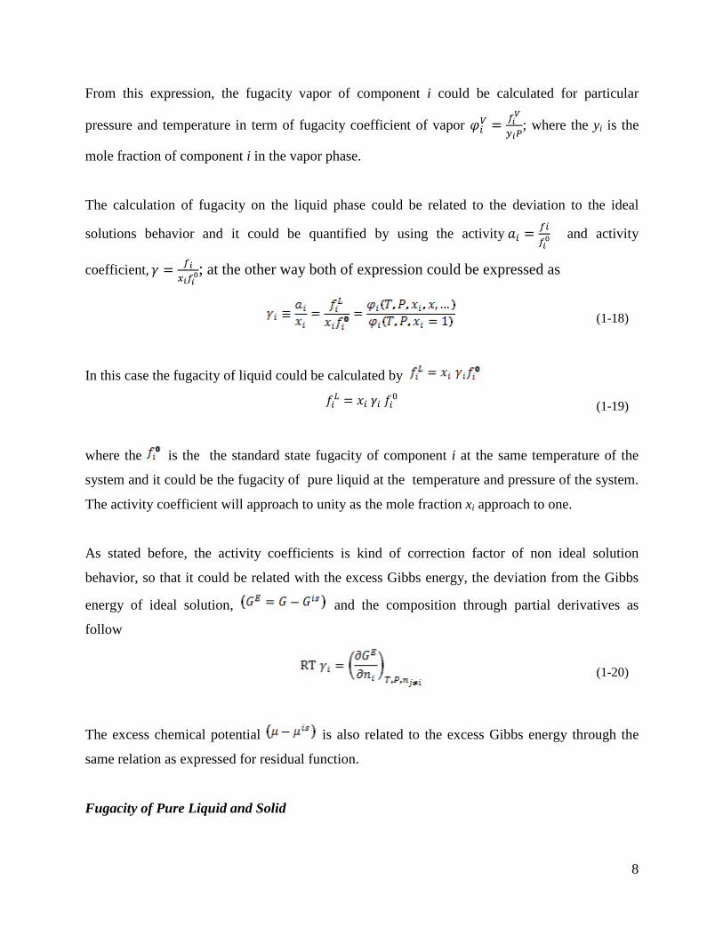
From this expression, the fugacity vapor of component i could be calculated for particular

pressure and temperature in term of fugacity coefficient of vapor ; where the yi is the

mole fraction of component i in the vapor phase.

The calculation of fugacity on the liquid phase could be related to the deviation to the ideal

solutions behavior and it could be quantified by using the activity and activity

coefficient ; at the other way both of expression could be expressed as

(1-18)

In this case the fugacity of liquid could be calculated by

(1-19)

where the is the the standard state fugacity of component i at the same temperature of the

system and it could be the fugacity of pure liquid at the temperature and pressure of the system.

The activity coefficient will approach to unity as the mole fraction xi approach to one.

As stated before, the activity coefficients is kind of correction factor of non ideal solution

behavior, so that it could be related with the excess Gibbs energy, the deviation from the Gibbs

energy of ideal solution, and the composition through partial derivatives as

follow

(1-20)

The excess chemical potential is also related to the excess Gibbs energy through the

same relation as expressed for residual function.

Fugacity of Pure Liquid and Solid

9

For calculating the fugacity of component in the mixture, it requires information of fugacity of

pure component, at the same temperature. The fugacity of liquid could be calculated based on

poynting method and also equation of state method.

The poynting method is calculated by introducing poynting correction for the fugacity on the

saturation condition, expresses as

(1-21)

For the calculation of the saturation condition, the saturated liquid volume could be calculated

using the Rackett equation and also for the calculation of saturated vapor pressure, the Clausius

Calpeyron equation or Antonie equation could be used over particular range of pressure.

The solid fugacity of pure component also could be calculated the same as liquid phase, using

the poynting method but using the volume of solid phase.

(1-22)

2 Phase Equilibrium by Equation of State As on the pure component, the basic equation of state does not change for mixture application. In

addition it requires extension to incorporate the compositional dependence for the mixture. For

brief discussion, the discussion will be limited to the cubic equation of state and quadratic

mixing rule application.

2.1 Cubic Equation of State There have been developed many equations of state for modeling phase equilibria. For particular

case, we use the Soave Redlich Kwong equation of state which is common for hydrocarbon

mixture phase equilibrium application. SRK is one of the cubic equation of state, that for solving

the total volume for a give information of pressure and temperature, third power equation of

density.

10

The SRK equation of state [1, 2] which relate the pressure, temperature, and also volume

expressed as follow

vbv

Tabv

RTp)()(

+−

−= (2-1)

The equation could be re-written into third power form

0223 =−

−−+−

pabv

pRTbb

pav

pRTv (2-2)

By evaluating at the critical pressure, the equation could be solved for a and b for each i

component on the system

ic

ici p

RTb

,

,08664.0=

ic

ici p

TRa

,

,2

08664.0and = (2-3)

Where for certain temperature other than the critical temperature

)()( TaTa ii α=

)1(1)( 5.0ri TcT −+=α

217.0547.1480.0 iiic ωω −+=

(2-4)

2.2 Mixing Rules Basically the mixing rule represent the molecular interaction among the molecules which extent

the application of equation of state to the multi component phase equilibria. On of the common

mixing rule is the quadratic mixing rule which originally proposed by Van der Walls based on

the principal of statistical mechanics. The quadratic mixing rule simply defined as follow

(2-5)

11

The component represents the molecular volumes average of the mixture and the parameter

represents the energy interaction among the molecules. The combining rule is required on

parameter i.e. if the and molecule are not chemically identical so it is necessary to predict

the properties of the mixture due to the intermolecular forces between different molecules, and it

is defined by

(2-6)

where the is referred as the binary interaction parameter provided by fitting to experiment

result.

2.3 Application of EOS to Phase Equilibrium As already explained briefly on the equilibrium criteria where whole Gibbs energy is minimized,

so that chemical potential each phases for particular component should be equal.

And also it has been introduced about the relation between the residual Gibbs energy to the

chemical potential and also fugacity coefficient. In addition, it has been introduced too about the

residual Helmholtz energy for calculating the chemical potential when temperature and volume

is preferred.

(2-7)

By substitution of SRK equation of state into the equation above and integrate it over the range

(2-8)

For simply written equation, the A and B defined as follow

(2-9)

12

The fugacity coefficient is obtained by partial differential of residual Helmholtz energy is

(2-10)

Where the is the partial mole derivatives of A

(2-11)

By remembering the relation between fugacity coefficient and derivatives of residual Helmholtz

energy; and direct substitution for residual Helmholtz energy

derivatives term, the fugacity coeffieint for vapor and liquid phase could be introducing for

mole fraction of vapor and for mole fraction of the liquid phase. The last term is the

correction of ideal gas Helmohltz energy from V to Vig.

3 Phase Equilibria on Flash Calculation

One of the application thermodynamic equilibria is on the phase separation process on the flash

drum. In this case the fluid with total mass, F with z feed composition entering into the flash

drum which conditioned at particular temperature and pressure.

The fluid contain of vapor and liquid so that based on the overall mass balance we may write

(3-1)

so that it is also applicable that ;

13

And for the component balance, the fraction of component contained inside the fluid mixture

could be written as

(3-2)

where the and ;

For the system under equilibrium, i.e. vapor liquid equilibrium, the fugacity of the phases will be

equal for each component. So that it also possible to define the ratio between liquid to vapor

mole fraction as follow:

(3-3a)

(3-3b)

(3-3c)

For each phase, the total mole fraction would be unity, so it could be written as

(3-4)

and from both relation, by applying the symmetric condition we find that, for vapor phase

(3-5)

By substitution for and , derived from the component balance

(3-6)

by substitution of

(3-7)

14

and substitution to the symmetric condition,

(3-8)

(3-9)

Since we coul rewrite the equation as

(3-10)

To solve the phase equilibrium requires step of iteration, based on the mass balance and also

equilibrium criteria.

Following subchapter will provide information on how solving based on k-ratio method if the

know parameter temperature and pressure, or temperature and total volume.

Another method will be also introduced on solving the phase equilibria using EOS, the Newton

method.

3.1 The K-ratio method

The following will discuss on how to find the composition of vapor and liquid mixture using the

k-ratio method if precondition of volume or pressure are known, for particular temperature.

The equation involved basically by solving the chemical potential balance and also the mass

balance over the system. If we look back on the SRK equation of state (eq. 2-1), the equation is

required to calculate the fugacity coefficient, by following steps

15

, ,ˆln ( ) ln

ji T V ni

F Zn

ϕ ∂= −

∂ (3-11)

where the F function is defined as ( , , )rA T VFRT

=n

, it also could be written as

( , , ) 1 ( )

r VA T V nRTF P dVRT RT V∞

= = − −∫n

(3-12)

Other form of SRK EOS by introducing extensive variable ( ,n V ) instead of intensive variable

for the volume and mole ( ,x v ) the SRK EOS (eq. 2-1) become

1 2( )( )nRT AP

V B V c B V c B= −

− + + (3-13)

where the Vvn

= , ii

nxn

= , and and

And also for the mixing rule as follow

2 2

11i j ij i j ij

i j i ja x x a n n a An n= = =∑∑ ∑∑ (3-14a)

i j ij

i jA n n a=∑∑

i i

iB n b=∑

(3-14b)

11i i i i

i ib x b n b Bn n= = =∑ ∑

(3-14c)

Substitution eq. 3-13 into eq. 12 to have the residual Helmholtz energy as follow

1 2

1 [ ]( )( )

V nRT A nRTF dVRT V B V c B V c B V∞

= − − −− + +∫

(3-15)

By solving the integration And the finial expression of eq.(3-15) after integration of the right

hand is: 1

2 1 2

ln ln( )

V c BV AF nV B RTB c c V c B

+= +

− − + (3-16)

16

The fugacity coefficient is function of derivation residual Helmholtz energy, i

Fn∂∂

. From eq.(3-

16), we can get set ( , , , , )F F T V n A B= , for T and V are constant, then

i i i i

F F n F A F Bn n n A n B n∂ ∂ ∂ ∂ ∂ ∂ ∂

= + +∂ ∂ ∂ ∂ ∂ ∂ ∂

(3-16)

Where the each part of the derivative on the eq. 3-16 are defined as follow

1

i

nn∂

=∂

(3-17a)

ln( )F V

n V B∂

=∂ −

(3-17b)

1

2 1 2

1 ln( )

V c BFA RTB c c V c B

+∂=

∂ − +

(3-17c)

1

1 2 22

2 1 1 2 2 1

ln( )

( ) ( )

V c BAc c V c BF n A

B n B RTB c c V c B V c B RTB c c

++∂

= + − −∂ − − + + −

(3-17d)

2 i j j

ji

A a nn∂

=∂ ∑

(3-17e)

i

i

B bn∂

=∂

(3-17f)

By direct substitution of each derivative into eq. 3-16, it would give the same result as eq. 2-10

and eq. 2-12.

3.1.1 Solve the SRK EOS To calculate the fugacity coefficient in the previous part, it is necessary to solve eq. 2-2 to get

volume, , i.e. of VLE, for both vapor and liquid. In more general form the eq.2-2 can be

rearranged as

3 2

2 12

1 2 1 1 23 2

1 2 1 2

[ ( ) ]

{[ ( ) ( ) ] / }

{( ) / ] 0

v c b c b b RT vP c b b c b Pc b RT c b c b a P v

Pc c b RTc c b ab P

+ + − −

+ − − − + +

+ − − − =

(3-18)

17

For given pressure P and temperature T, the cubic equation eq. 3-18 can be solved to get , and

we may get just one real root or three real roots.

In the situation of three real roots, it is necessary to determine the stable root according to

thermodynamic theory. The minimum Gibbs energy solution also corresponding to the

minimum residual Gibbs energy solution, it is possible to choose the stable root for v where eq.3-

19 is the smallest value.

( 1 ln )resG F n Z Z

RT= + − − (3-19)

18

3.1.2 Algorithm for the Two Phase TPn (isothermal) flash

Figure 1 TPn vapor liquid flash algorithm using K ratio method

Given T, P and feed composition z

Calculate

Solve Rachford-Rice equation

for phase fraction vapor fraction

Vapor comp.:

Liquid comp.:

Convergence?

No

Yes

Finish calculation

19

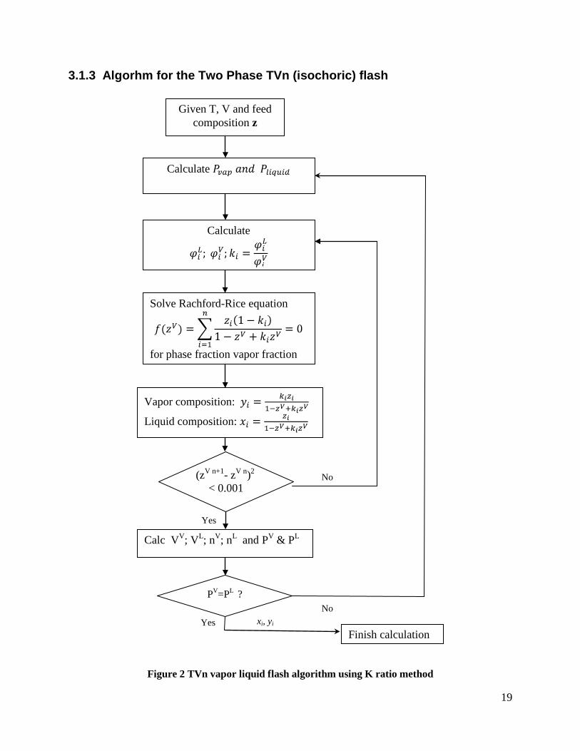
3.1.3 Algorhm for the Two Phase TVn (isochoric) flash

Figure 2 TVn vapor liquid flash algorithm using K ratio method

Given T, V and feed composition z

No

Yes Calc VV; VL; nV; nL and PV & PL

Calculate

Finish calculation

Calculate

Solve Rachford-Rice equation

for phase fraction vapor fraction

Vapor composition:

Liquid composition:

(zV n+1- zV n)2 < 0.001

PV=PL ? No

Yes

Yes

xi, yi

20

3.2 Freezing Temperature

Based on the previous K-ratio algorithm, for given temperature, feed composition, and also

volume or pressure, we can solve the equilibrium equations get the composition of vapor and

liquid. For thermodynamic equilibrium calculation by using cubical EOS, where the pressure is

low and it is also possible to calculate the fugacity of vapor and liquid by using

i i if x Pϕ= (3-20)

In this case ix is the concentration of the component i in fluid (liquid or vapor).

Assume the freeze out component is pure solid, if the solid fugacity is equal to or smaller than

the fugacity of the corresponding component in the liquid or vapor, then there will be freeze out

solid, which is

solid Fi if f<= (3-21)

Here Fif denotes the fugacity of component i in the liquid mixture or vapor mixture. To express

the solid fugacity in a simple way, we can use the pointing method, which is

( )exp( )s sat

s sat sat v P Pf PRT

ϕ −= (3-22)

Where satP are the sublimation pressure the component at temperature T, and satϕ is the fugacity

coefficient of the vapor at temperature T and pressure satP .

One of simple way in this exercise, the sublimation pressure can be calculated from Clausius-

Claperyon

2

1 1 2

1 1ln( ) ( )P hP R T T

∆= − (3-23)

h∆ is the enthalpy difference between the solid and the vapor at the sublimation line.

21

3.3 The Newton Method

3.3.1 TVn Flash Using Newton Method Given temperature T, the feed mole amount of each component n and also the feed volume V,

the necessary condition for liquid vapor equilibrium is equal chemical potential of individual

component in each phase and equal pressure in the system, which is:

α βµ µ= (3-24a)

P Pα β= (3-24b)

Here α and β are corresponding to vapor phase and liquid phase. The pressure can be

expressed as derivatives of Helmholtz energy and eq. 3-24a becomes

V VA Aα β= (3-25)

Use the Newton method to solve eq. 3-24b and eq.3-25 the matrix formulation is:

V n V nV Vα α α α α β β β β βµ µ µ µ µ µ+ ∆ + ∆ = + ∆ + ∆n n (3-26)

V VV Vn V VV VnA A V A A A V Aα α α α α β β β β β+ ∆ + ∆ = + ∆ + ∆n n (3-27)

α β−∆ = ∆n n (3-28)

V Vβ α−∆ = ∆ (3-29)

of liner equation, we can get

( )( )

TVV VV V V V V

V V

A A V A Aα β α β α α β

α β α β α α β

µ µµ µ µ µ

+ + ∆ −= −

+ + ∆ − A A n (3-30)

Here 2,{( / ) }i j T VA N N= ∂ ∂ ∂A .

Use eq.3-30 to solve the TVn flash, it is necessary to get the second derivatives of the Helmholtz

energy.

Second derivatives of Helmholtz energy

22

It is quite often to split the Helmholtz energy into residual part and ideal gas part, which is

res igA A A= + (3-31)

As in the K ratio method part, we define

( , , )resA T VFRT

=n

(3-32)

Substitute eq. (3-17a) into eq.(3-16), we can get

i i i

F F F A F Bn n A n B n∂ ∂ ∂ ∂ ∂ ∂

= + +∂ ∂ ∂ ∂ ∂ ∂

(3-33)

The derivatives of Helmholtz energy are calculated the following part.

(3-34)

The value of i

Fn∂∂

can be calculated from eq. (3-33) together with eq.(3-17b-17f).

2 2 2

, , ,

res ig

i j i j i jT V T V T V

A A An n n n n n

∂ ∂ ∂= + ∂ ∂ ∂ ∂ ∂ ∂

(3-35)

2

,,

( ( ) ln ) 1( )i

ig iij

i j j iT VT V

nT RTA nn n n n N

µ δ ∂ + ∂

= = − ∂ ∂ ∂

(3-36)

ijδ is the Kronecker parameter, where 1ijδ = when i j= and 0ijδ = when i j≠ .

2 2

, ,

res

i j i jT V T V

A FRTn n n n

∂ ∂= ∂ ∂ ∂ ∂

(3-37)

2

,i j T V

Fn n

∂ ∂ ∂

can be calculated from eq.(3-33), the first derivatives, so the second derivatives

become

23

2

,

2 2 2 2 2

i j T V

j j i i j j i i j

Fn n

F F A F A F B F Bn n A n n A n n B n n B n n

∂= ∂ ∂

∂ ∂ ∂ ∂ ∂ ∂ ∂ ∂ ∂+ ⋅ + ⋅ + ⋅ + ⋅ ∂ ∂ ∂ ∂ ∂ ∂ ∂ ∂ ∂ ∂ ∂ ∂ ∂ ∂

(3-38)

From eq. (3-17b) and eq.(3-17f), we have

2

j

j

bFn n V B∂

=∂ ∂ −

(3-39)

From eq.(3.17c) and eq.(3-17b), we have

21

22 1 2

1 2

2 1 1 2

ln( )

1 [ ]( )

j

j

j j

b V c BFA n RTB c c V c B

c b c bRTB c c V c B V c B

+∂= − ⋅ ∂ ∂ − +

+ ⋅ −− + +

(3-40)

From eq.(3-17e), we get

2

2 iji j

A an n∂

=∂ ∂

(3-41)

From eq. (3-17f), we get

2

0i j

Bn n∂

=∂ ∂

(3-42)

From eq.(3.39-42), we get

24

2

2

2 1 2 11 2

22 1 1 2

1 2 32 2

2 1

( )(2 )[ ( )] ( )

[ ]( )

[ ( )]

j

j

jk k jk

FB nB nbn B

a n RTB c c ARTb c cc c

RTB c c V c B V c BX X X

RTB c c

∂=

∂ ∂

− +

−

− − −+ −

− + ++ +

−−

∑ (3-43)

Where

11

2

(2 ) lnjk kk

V c BX a nV c B+

=+∑ (3-44a)

1 2 22 2 1

1 2

( ) ( )j jc b c bX A RTB c c

V c B V c B= − −

+ + (3-44b)

13 2 1

2

2 ( ) lnjV c BX RTB c c b AV c B+

= −+

(3-44c)

Substitute eq.(3-17a-3.17f) and eq.(3-39-44c) to eq.(3-38), and substitute eq.(3-36-38) into eq.(3-

35), we can get 2

,i j T V

An n

∂ ∂ ∂

.

Use eq.(14), we can get

, 1 2( )( )n T

A nRT APV V B V c B V c B∂ = − = − + ∂ − + +

(3-45)

21 2

2 2 21 2,

(2 )( ) [( )( )]n T

A V c B c BA nRTV V B V c B V c B

+ +∂= − ∂ − + +

(3-46)

1 2 1 2 1 2

2 21 2

(2 )( )( ) [( ) 2 ]

( ) [( )( )]

V i ii n V Vn

i j j j iji

A A

a n V c B V c B A c c Vb c c BbnRTb

V B V c B V c B

µ = =

+ + − + +−

= +− + +

∑ (3-47)

25

Substitute the above derivatives into eq.(3-26-27), we can calculate the Newton step.

3.3.2 TPn Flash Using Newton Method For the TPn flash using Newton method, the procedure is quite similar to the TVn flash, but in

this case, pressure P is given, can we have to find the volume for the vapour and the liquid. The

given pressure can be expressed as:

0( , , )P T V Pα α =n (3-48)

0( , , )P T V Pβ β =n (3-49)

Where 0P is the specified pressure. Linearization of the two equations can be expressed as:

0VP P V P Pα α α α+ ∆ + ∆ =n n (3-50)

0VP P V P Pβ β β β+ ∆ + ∆ =n n (3-51)

In the TPn flash, we still solve the eq. 3-30 in iteration to update mole amount of each

component in the liquid and vapour phase, and also we can get the update volume of the vapour

and liquid, then by using eq. 3-50 and eq. 3-51, we can update the pressure for vapour and liquid

phase. The new volume for eq 3-30 is calculated from solving the cubic SRK equation for

volume, that is eq 3-18. The algorithm is also shown in Fig 3.

26

Figure 3 TPn vapor liquid flash algorithm using Newton method

Given T, P and feed composition z

Calculate V vapor and V liquid By eq. 3-18

Solve eq. 3-30, get the step for volume and mole amount

, , ,V Vα β α β∆ ∆ ∆ ∆n n

V V VV V V

α α α

β β β

= + ∆

= + ∆

α α α

β β β

= + ∆

= + ∆

n n nn n n

0

0

V

V

P P P V PP P P V P

α α α α

β β β β

= − ∆ − ∆

= − ∆ − ∆n

n

nn

Convergence?

No

Yes

Finish calculation

27

3.4 Result and Discussion

The vapor liquid flash and the freezing temperature calculations are implemented in matlab, the calculation results are shown as follows.

3.4.1 Comparision between Pro.II and TPn K-ratio Method

In this exercise, the vapor liquid equilibrium for given composition of gas, is solved using SRK

EOS. And then the result is compared to the same model SRK provided by commercial software.

Both for the TVn and TPn flash are compared. In this case the commercial software used is Pro

II.

The bubble point line and due point line calculated by ProII for a gas mixture is shown in Fig. 3,

the components and composition of the mixture are shown in table 1. In this work, the PTn flash

calculation of two points in the two phase liquid-vapor region using K ratio method is compared

with the calculation from ProII, and the results are shown in table 1 and table 2.

Figure 4 PT phase diagram of gas mixture calculated by ProII

Temperature, K0 60.0 120.0 180.0 240.0 300.0

Pres

sure

, MPa

0

2.50

5.00

7.50

10.00

12.50

Phase Envelope Curve for stream 'S1', Description :

Full EnvelopeLiquid Mole Fraction : 0.000000Critical PointCricondenbarCricondentherm

28

For given gas composition, and pressure at 1 Mpa and temperature is 170K, the mole fraction for

each phases, compared for calculation using Matlab and Pro. II as follow:

Table 1 Comparision of results between ProII and this work: PTn flash using K ratio methd at 1Mpa, 170K

No. Composition

inlet composition

(zi)

Vapor (yi) Liquid (xi)

Pro.II This work Pro.II This work 1 Methane 0.80000 0.89300 0.88857 0.33660 0.35598 2 Ethane 0.05000 0.01360 0.01403 0.23120 0.23031 3 Propane 0.03000 0.00072 0.00072 0.17600 0.17679 4 Hexane 1.000E-02 8.036E-08 0.000E+00 5.980E-02 6.013E-02 5 N2 0.05000 0.05950 0.05937 0.00251 0.00301 6 CO2 0.06000 0.03310 0.03730 0.19380 0.17378

At higher pressure that the critical point, the consistency of the result for this exercise indicates

slightly differences compared to the Pro. II result. Table 2 Comparision of results between ProII and this work: PTn flash using K ratio methd at 10Mpa, 170K

No. Composition

inlet composition

(zi)

Vapor (yi) Liquid (xi)

Pro.II This work Pro.II This work 1 Methane 0.80000 0.80620 0.80484 0.57370 0.63214 2 Ethane 0.05000 0.04880 0.04897 0.09310 0.08571 3 Propane 0.03000 0.02820 0.02840 0.09750 0.08571 4 Hexane 1.000E-02 6.519E-03 7.305E-03 1.374E-01 1.036E-01 5 N2 0.05000 0.05090 0.05082 0.01880 0.02143 6 CO2 0.06000 0.05950 0.05967 0.07960 0.07143

3.4.2 Verification of TVn flash by TPn flash of K ratio method

In the previous part, it is shown that the TPn flash calculation using K ratio method from this

work is comparable to the result from ProII, also, we can get the total volume from the TPn

flash.

To verify the TVn flash result, we can start the calculation by specifying the given volume

equals the volume we get from the TPn flash, and the temperature and feed composition equals

29

the given condition in the TPn flash calculation, if the implementation of the TVn flash

calculation is collect, we should get the pressure equals the given pressure in the TPn flash, and

the same vapor liquid composition as TPn flash.

Table 3 and table 4 are the results for the verification of the TVn flash by TPn flash, the feed in

table three for both TPn flash and TVn flash are the same as shown in table 4. The results show

that the TVn flash is verified by the TPn flash.

Table 3 Verification of TVn flash by TPn flash at 170K

TPn flash TVn flash Given

condition Temperature (K) 170 170 Pressure (MPa) 1.0000 Total Volume (m3) - 0.0010552

Calculation result

Pressure (MPa) - 1.0000MPa Total Volume (m3) 0.0010552 -

Table 4 Verification of TVn flash by TPn flash: Vapor and Liquid composition at 1MPa, 170K

No. Composition

inlet composition

(zi)

Vapor (yi) Liquid (xi)

TPn TVn TPn TVn 1 Methane 0.80000 0.89300 0.88850 0.33660 0.35624 2 Ethane 0.05000 0.01360 0.01408 0.23120 0.23010 3 Propane 0.03000 0.00072 0.00071 0.17600 0.17688 4 Hexane 1.000E-02 8.036E-08 8.675E-08 5.980E-02 6.014E-02 5 N2 0.05000 0.05950 0.05942 0.00251 0.00279 6 CO2 0.06000 0.03310 0.03729 0.19380 0.17386

3.4.3 Comparison K ration method and Newton method

The comparison between two method, K-ratio and Newton method has been performed. By

using both method, it has been performed for TVn flash and TPn flash for the same composition.

The same result has been gain for both method, and the result also being used for validation

between TVn and TPn.

30

The convergence analysis is indicated by curve below for the K-ratio and the Newton method. It

shows that the K-ratio method is first order convergent and Newton method is second order

convergent.

Figure 5 Convergence analysis of K ratio mehod

Figure 6 Convergence analysis of Newton method

31

3.4.4 Freeze out temperature prediction

Measurement for freeze out temperature of CO2 – Methane mixture has been performed Le. [3].

In this case, we would like to compare the calculation result in this exercise with the

experimental data. The focus would be on the low concentration of CO2 and higher pressure

condition.

The experiment performed by Le was Solid Vapor Equilibrium for three type of concentration of

CO2 in CO2-CH4 mixture, 1%, 1.91% and 2.93% of CO2.

The model by using SRK EOS on modeling the Solid Vapor indicates slight deviation to the

experiment result. For higher pressure, the deviation is high. In this exercise, the binary

interaction parameters being used are the binary interaction parameter for liquid vapor

equilibrium which can cause the deviation when it is applied for solid vapor equilibrium.

CO2 1.00 % Pressure

(kPa) Temp (K)

Le(1) Temp (K)

Calculated 1109.5 170.5 167.99 1435.2 173.6 169.71 1809.1 175.5 173.79 2129.2 177 177.5 2464.2 177.8 181.1

Table 5 Comparison between experiment result and SRK EOS on solid vapor equilibrium

CO2 1.91 % Pressure

(kPa) Temp (K)

Le(1) Temp (K)

Calculated 1375.9 175.99 173.8 1705.1 178.06 176.9 2135.3 183.06 181 2651.5 188.27 186.3 3008.2 191.5 187.7

CO2 2.93 % Pressure

(kPa) Temp (K)

Le(1) Temp (K)

Calculated 1199 176.5 179.4

1421.4 179.1 180.7 1683.6 181.9 182.3 1982.4 183 185.8 2428.4 185.3 190.6

32

From the table, the deviation to the experiment result 1-3%, high deviation especially found at

low concentration and high pressure. It indicates that the model could predict the freeze out even

less accurate, but adjustment on the interaction parameter and also on the enthalpy of fusion is

expected to have better result.

Comparison for Liquid-solid phase equilibrium between the model and experimental data (GPA

RR-10 Report) has been done for solid CO2 in liquid of methane. Slight difference on the

prediction can be observed on the curve below.

0

5

10

15

20

160 170 180 190 200 210

Calculation by this work

Experimental data

CO2

mol

%

Temperature (K)

Figure 7 Solubility of CO2 in liquid CH4[2]

4 Conclusion and suggested further work

4.1 Conclusion In this work, the background of the equilibrium calculation is introduced, followed by the

thermodynamic framework of phase equilibrium. To show the practical calculation aspects, both

the TPn and TVn flash calculations are carried out using K ratio and Newton method, as shown

33

in table 6. The calculations are implemented in matlab and the calculation results are verified by

commercial software PROII and also by experimental data.

The prediction of solid-vapor-liquid phase behavior is illustrated through the freeze out

prediction of CH4-CO2 system, the calculation results was reasonable compared to experimental

data. Table 6 Flash calculations in this work

Methods TPn flash TVn flash

K ratio method × ×

Newton mehod × ×

4.2 Suggested further work This project work shows the basic feathers in the calculation of gas mixture phase behavior, but

to make the simulation accurate for real situation, there are still a lot of work left to be done

based on this project, the following topics are suggested to be done to predict the natural gas

mixture phase behavior (include solid phase) at low temperature:

• Implement the stability analysis and multiphase equilibrium algorithm.

• Implement more accurate thermodynamic model, for example, to get the binary

interaction parameters accurate for the cubic EOS, or to implement other thermodynamic

models for the fluid phase such as GERG-2004, and also improve the thermodynamic

model for the solid.

References 1. Soave, G.S., Application of the Redlich-Kwong-Soave Equation of State to Solid-Liquid

Equilibria Calculations. Chemical Engineering Science, 1979. 34(2): p. 225-229. 2. Kurata, F., Research Report RR-10 Solubility of Solid Carbon Dioxide in Pure Light

Hydrocarbons and Mixtures of Light Hydrocarbon. 1974. 3. Le, T.T. and M.A. Trebble, Measurement of carbon dioxide freezing in mixtures of

methane, ethane, and nitrogen in the solid-vapor equilibrium region. Journal of Chemical and Engineering Data, 2007. 52(3): p. 683-686.

34

4. Elliott, J.R. and C.T. Lira, Introductory chemical engineering thermodynamics. Prentice-Hall international series in the physical and chemical engineering sciences. 1999, Upper Saddle River, NJ: Prentice Hall PTR.

5. Prausnitz, J.M., E.G.d. Azevedo, and R.N. Lichtenthaler, Molecular thermodynamics of fluid-phase equilibria. Prentice-Hall international series in the physical and chemical engineering sciences. 2004, Upper Saddle River, NJ: Prentice Hall PTR.

6. Michelsen, M.L. and J.r.M. Mollerup, Thermodynamic models : fundamentals & computational aspects. 2004, Holte, Denmark: Tie-Line Publications.

7. Tore Haug-Warberg, Lecture Note- KP8108 Advanced Thermodynamics: with applications to Phase and Reaction Equilibria, October 20, 2008; Department of Chemical Engineering, NTNU

35

Appendix: Source code for TPn Newton flash (The algorithm is shown in fig. 3)

1. Main program % Program for (T,V) flash using Newton Method. % component vector (CH4, C2H6, C3H8, C6H14, N2, CO2); T = 170; % K P0=1.0e+6; % Initial value of the vapor and liquid phase n_vapor =[ 0.7 0.0117 0.0006 0.00000007232679 0.0495 0.0311]; n_liquid =[ 0.1 0.0383 0.0294 0.0100 0.0005 0.0289]; n = n_vapor+n_liquid; Vaporfraction_initial = sum(n_vapor)/sum(n); P_vapor=P0; P_liquid=P0; %----------------------------------------------------------------- % Solve the Newton iteration error= 1000; lhs=zeros(7); rhs=zeros(7,1); delta_step=zeros(7,1); iteration=0; while error > 0.000000001 iteration=iteration+1; V_vapor = GetV(P_vapor,n_vapor,T,-1); V_liquid = GetV(P_liquid,n_liquid,T,1); P_v_vapor=P_V(V_vapor,n_vapor,T); P_v_liquid=P_V(V_liquid,n_liquid,T); P_ni_vapor=P_ni(V_vapor,n_vapor,T); P_ni_liquid=P_ni(V_liquid,n_liquid,T); A_vv_vapor=AVV(V_vapor,n_vapor,T); A_vv_liquid=AVV(V_liquid,n_liquid,T); Mu_v_vapor=MU_V(V_vapor,n_vapor,T); Mu_v_liquid=MU_V(V_liquid,n_liquid,T); A_ninj_vapor=A_NINJ(V_vapor,n_vapor,T); A_ninj_liquid=A_NINJ(V_liquid,n_liquid,T); A_v_vapor=A_V(V_vapor,n_vapor,T); A_v_liquid=A_V(V_liquid,n_liquid,T);

36

Muvapor_minus_Muliquid=Mu_dif(V_liquid,n_liquid,V_vapor,n_vapor,T); lhs(1,1) = A_vv_vapor + A_vv_liquid; lhs(1,2:end) = Mu_v_vapor + Mu_v_liquid; lhs(2:end,1) = Mu_v_vapor + Mu_v_liquid; lhs(2:end,2:end) = A_ninj_vapor + A_ninj_liquid; lhs; rhs(1) = -(A_v_vapor-A_v_liquid); rhs(2:end) = -(Muvapor_minus_Muliquid); rhs; delta_Step_old= delta_step; delta_step=lhs\rhs; error=sum((delta_Step_old-delta_step).^2); P_vapor=P0-P_v_vapor*delta_step(1,1)-sum(P_ni_vapor'.*delta_step(2:end,1)); P_liquid=P0+P_v_liquid*delta_step(1,1)+sum(P_ni_liquid'.*delta_step(2:end,1)); for i=1:6 n_vapor_new(i)=n_vapor(i)+delta_step(i+1,1); n_liquid_new(i)=n_liquid(i)-delta_step(i+1,1); end n_vapor_new; n_liquid_new; while ~(min(n_vapor_new) >= 0 & min(n_liquid_new) >= 0) display('n is negative ,Decrease the step size to 40%'); delta_step=0.4*delta_step; P_vapor=P0-P_v_vapor*delta_step(1,1)-sum(P_ni_vapor.*delta_step(2:end,1)); P_liquid=P0+P_v_liquid*delta_step(1,1)+sum(P_ni_liquid.*delta_step(2:end,1)); for i=1:6 n_vapor_new(i)=n_vapor(i)+delta_step(i+1,1); n_liquid_new(i)=n_liquid(i)-delta_step(i+1,1); end n_vapor_new; n_liquid_new; end n_vapor=n_vapor_new; n_liquid=n_liquid_new; Beta=sum(n_vapor)/sum(n); y= n_vapor/sum(n_vapor); x= n_liquid/sum(n_liquid);

37

P_liquid P_vapor end display ('***************************TVn flash is solved') display ('************ The input:') T n display ('************ The result:') iteration V_vapor V_liquid n_vapor n_liquid y= n_vapor/sum(n_vapor) x= n_liquid/sum(n_liquid) Beta=sum(n_vapor)/sum(n) P_liquid P_vapor

2. Function to calculate the SRK EOS parameters function [n_total,a_individual,b_individual,a_binary,a_mixture,b_mixture,A,B]=SRK_parameters(T,n) % Step 1: Calculate molor fraction x n_total=sum(n); x=n/sum(n); % Step 2: Input individual critical properties for each component % Critical properties Tcrit=[190.60 305.40 369.80 507.40 126.20 304.20]; Pcrit=[4.599 4.883 4.244 2.968 3.394 7.375]; Omega=[0.0080 0.0980 0.1520 0.2960 0.0400 0.2250]; % Interaction coefficients K_binary=zeros(6,6); K_binary(1,5)=0.02; K_binary(1,6)=0.12; K_binary(2,5)=0.06; K_binary(2,6)=0.15; K_binary(3,5)=0.08; K_binary(3,6)=0.15; K_binary(4,5)=0.08; K_binary(4,6)=0.15;

38

K_binary(5,1)=0.02; K_binary(5,2)=0.06; K_binary(5,3)=0.08; K_binary(5,4)=0.08; K_binary(6,1)=0.12; K_binary(6,2)=0.15; K_binary(6,3)=0.15; K_binary(6,4)=0.15; % Calculate the parameter a and b for individual components and mixture R_gasconstant = 8.314472; % m3*Pa/(K*mol) % a_individual for SRK EOS a_coefficient_individual = (1+(0.48+1.574*Omega- ... 0.176*Omega.^2).*(1-(T./Tcrit).^0.5)).^2; a_individual = 0.42748* ... (((R_gasconstant^2)* ... (Tcrit.^2)./(1000000*Pcrit))).*a_coefficient_individual; b_individual=0.08644 * R_gasconstant * Tcrit./(1000000*Pcrit); a_binary=zeros(6,6); for i=1:6 for j=1:6 a_binary(i,j)=(a_individual(i)*a_individual(j))^0.5*(1-K_binary(i,j)); end end clear i; clear j; a_mixture=0; b_mixture=0; for i=1:6 for j=1:6 a_mixture = a_mixture + x(i)*x(j)* a_binary(i,j); end b_mixture = b_mixture + x(i) * b_individual (i) ; end clear i; clear j; A = (n_total ^ 2)* a_mixture; B = n_total * b_mixture;

39

3. Function to calculate 2

,i j T V

An n

∂ ∂ ∂

function A_ninj=A_NINJ(V,n,T) [n_total,a_individual,b_individual,a_binary,a_mixture,b_mixture,A,B]=SRK_parameters(T,n); R_gasconstant = 8.314472; c1=1.0; c2=0.0; A_ninj=zeros(6); dFdn=log(V/(V-B)); dFdA=(1/(R_gasconstant*T*B*(c2-c1)))*log((V+c1*B)/(V+c2*B)); for i=1:6 sumpart=0. ; for j=1:6 sumpart=sumpart+a_binary(i,j)*n(j) ; end dA_dni(i)=2*sumpart; end dFdB=(n_total/(V-B))+ ... (A/(R_gasconstant*T*B*(c2-c1)))*( c1/(V+c1*B)-c2/(V+c2*B)) ... - (A*log((V+c1*B)/(V+c2*B)))/(R_gasconstant*T*B*B*(c2-c1)) ; dB_dni= b_individual ; % Calculate the second derivatives d2F_dndnj=b_individual/(V-B); d2F_dAdnj= -b_individual/(R_gasconstant*T*B^2*(c2-c1)) * log((V+c1*B)/(V+c2*B)) + ... (1/(R_gasconstant*T*B*(c2-c1)))* ... (c1*b_individual/(V+c1*B)-c2*b_individual/(V+c2*B)); d2A_dnidnj=2*a_binary; d2B_dnidnj=zeros(6); jsumpart=[0 0 0 0 0 0]; for j=1:6 for k=1:6 jsumpart(j)=jsumpart(j)+a_binary(j,k)*n(k) ; end end d2F_dBdnj_1part=(V-B+n_total*b_individual)/(V-B)^2;

40

d2F_dBdnj_2part= ((2*jsumpart*(R_gasconstant*T*B*(c2-c1))-A*R_gasconstant*T*b_individual*(c2-c1))/ ... (R_gasconstant*T*B*(c2-c1))^2)*(c1/(V+c1*B)-c2/(V+c2*B)); d2F_dBdnj_3part=(A/(R_gasconstant*T*B*(c2-c1)))*(-c1^2*b_individual/(V+c1*B)^2+c2^2*b_individual/(V+c2*B)^2); d2F_dBdnj_4part = -((2*jsumpart*log((V+c1*B)/(V+c2*B)) + A*(c1*b_individual/(V+c1*B)-c2*b_individual/(V+c2*B))) ... * R_gasconstant*T*B^2*(c2-c1)- 2*R_gasconstant*T*B*(c2-c1)*b_individual*A*log((V+c1*B)/(V+c2*B)))/ ... ( R_gasconstant*T*B^2*(c2-c1))^2; d2F_dBdnj= d2F_dBdnj_1part+ d2F_dBdnj_2part+ d2F_dBdnj_3part+ d2F_dBdnj_4part; d2F_dninj=zeros(6); for i=1:6 for j=1:6 d2F_dninj(i,j) = d2F_dndnj(j) + d2F_dAdnj(j)*dA_dni(i)+dFdA*d2A_dnidnj(i,j) + d2F_dBdnj(j)*dB_dni(i) + dFdB*d2B_dnidnj(i,j); end end Kronecker=zeros(6); for j=1:6 Kronecker(j,j)=1; end for i=1:6 for j=1:6 A_ninj(i,j)=R_gasconstant*T*(d2F_dninj(i,j)+(1/n(i))*Kronecker(i,j)); end end

41

4. Function to calculate ,T

AV∂

∂ n

function A_v=A_V(V,n,T) % Function for calculating derivative A with v % step 1: Get the SRK EOS parameters [n_total,a_individual,b_individual,a_binary,a_mixture,b_mixture,A,B]=SRK_parameters(T,n); R_gasconstant = 8.314472; % Set the parameters for SRK EOS in the general cubic equation c1=1.0; c2=0.0; %--------------------------------------------------------------------- % Step 2: Calculate the derivative A_v= -n_total*R_gasconstant*T/(V-B) ... + A/((V+c1*B)*(V+c2*B));

5. Function to calculate 2

2,T

AV

∂ ∂ n

function A_vv=AVV(V,n,T) % Function for calculating the second derivatives A_VV %-------------------------------------------------------------------------- % step 1: Get the SRK EOS parameters [n_total,a_individual,b_individual,a_binary,a_mixture,b_mixture,A,B]=SRK_parameters(T,n); R_gasconstant = 8.314472; % Set the parameters for SRK EOS in the general cubic equation c1=1.0; c2=0.0; %--------------------------------------------------------------------- % Step 2: Calculate the derivative A_vv=n_total*R_gasconstant*T/(V-B)^2 ... + (-A*(2*V+c1*B+c2*B))/((V+c1*B)*(V+c2*B))^2;

42

6. Function to calculate volume for SRK EOS function V=GetV(P,n,T,Icon) % Function for calculating V %-------------------------------------------------------------------------- % Get the SRK EOS parameters [n_total,a_individual,b_individual,a_binary,a_mixture,b_mixture,A,B]=SRK_parameters(T,n); R_gasconstant = 8.314472; % Set the parameters for SRK EOS in the general cubic equation c1=1.0; c2=0.0; % Solve the equation for V and choose V A3=1; A2=-1; A_inter=a_mixture*P/(R_gasconstant*T)^2; B_inter=b_mixture*P/(R_gasconstant*T); A1=A_inter-B_inter-B_inter^2; A0=-A_inter*B_inter; z_cubic_roots=roots([A3 A2 A1 A0]); v=(z_cubic_roots*R_gasconstant*T)/(P); %-------------------------------------------------------------------------- % Determine the stable root % Take out the real roots from v v_imag=imag(v); if sum(v_imag.^2) == 0 ; % the image of v is zero, all three are real roots. v_intermid=v ; else for i=1:3 if imag(v(i))==0 v_intermid=v(i); end end end ; if length(v_intermid)==1 ; % only one real root v_stable=v_intermid ; else % three roots are real roots, we have to choose the stable one, % Only have to choose between the max one and the min one v_max=max(v); v_min=min(v); V1=n_total*v_min; F1_first_term=n_total*log(V1/(V1-B)); F1_second_term=(A/(R_gasconstant*T*B*(c2-c1)))*log((V1+c1*B)/(V1+c2*B)); F1_value=F1_first_term+F1_second_term; Z1=((P)*v_min)/(R_gasconstant*T); G_vmin_reducedres=F1_value+n_total*(Z1-1-log(Z1)); % calculate the v_max coressponding Reduced Resudual Gibbs energy V2=n_total*v_max; F2_first_term=n_total*log(V2/(V2-B)); F2_second_term=(A/(R_gasconstant*T*B*(c2-c1)))*log((V2+c1*B)/(V2+c2*B)); F2_value=F2_first_term+F2_second_term; Z2=((P)*v_max)/(R_gasconstant*T);

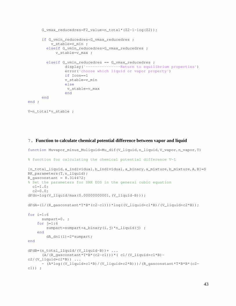
43

G_vmax_reducedres=F2_value+n_total*(Z2-1-log(Z2)); if G_vmin_reducedres<G_vmax_reducedres ; v_stable=v_min ; elseif G_vmin_reducedres>G_vmax_reducedres ; v_stable=v_max ; elseif G_vmin_reducedres == G_vmax_reducedres ; display('---------------Return to equilibrium properties') error('choose which liquid or vapor property') if Icon==1 v_stable=v_min else v_stable=v_max end end end ; V=n_total*v_stable ;

7. Function to calculate chemical potential difference between vapor and liquid function Muvapor_minus_Muliquid=Mu_dif(V_liquid,n_liquid,V_vapor,n_vapor,T) % function for calculating the chemical potential difference V-L [n_total_liquid,a_individual,b_individual,a_binary,a_mixture,b_mixture,A,B]=SRK_parameters(T,n_liquid); R_gasconstant = 8.314472; % Set the parameters for SRK EOS in the general cubic equation c1=1.0; c2=0.0; dFdn=log(V_liquid/max(0.00000000001,(V_liquid-B))); dFdA=(1/(R_gasconstant*T*B*(c2-c1)))*log((V_liquid+c1*B)/(V_liquid+c2*B)); for i=1:6 sumpart=0. ; for j=1:6 sumpart=sumpart+a_binary(i,j)*n_liquid(j) ; end dA_dni(i)=2*sumpart; end dFdB=(n_total_liquid/(V_liquid-B))+ ... (A/(R_gasconstant*T*B*(c2-c1)))*( c1/(V_liquid+c1*B)-c2/(V_liquid+c2*B)) ... - (A*log((V_liquid+c1*B)/(V_liquid+c2*B)))/(R_gasconstant*T*B*B*(c2-c1)) ;

44

dB_dni= b_individual ; dF_dni_liquid=dFdn+dFdA*dA_dni+dFdB*dB_dni; clear a_individual b_individual a_binary a_mixture b_mixture A B [n_total_vapor,a_individual,b_individual,a_binary,a_mixture,b_mixture,A,B]=SRK_parameters(T,n_vapor); R_gasconstant = 8.314472; c1=1.0; c2=0.0; dFdn=log(V_vapor/(V_vapor-B)); dFdA=(1/(R_gasconstant*T*B*(c2-c1)))*log((V_vapor+c1*B)/(V_vapor+c2*B)); for i=1:6 sumpart=0. ; for j=1:6 sumpart=sumpart+a_binary(i,j)*n_vapor(j) ; end dA_dni(i)=2*sumpart; end dFdB=(n_total_vapor/(V_vapor-B))+ ... (A/(R_gasconstant*T*B*(c2-c1)))*( c1/(V_vapor+c1*B)-c2/(V_vapor+c2*B)) ... - (A*log((V_vapor+c1*B)/(V_vapor+c2*B)))/(R_gasconstant*T*B*B*(c2-c1)) ; dB_dni= b_individual ; dF_dni_vapor=dFdn+dFdA*dA_dni+dFdB*dB_dni; Muvapor_minus_Muliquid = R_gasconstant*T*(dF_dni_vapor+log(n_vapor/V_vapor)) - ... R_gasconstant*T*(dF_dni_liquid+log(n_liquid/V_liquid));

8. Function to calculate Vµ∂∂

function Mu_v=MU_V(V,n,T) % Function for calculating the second derivatives A_Vni [n_total,a_individual,b_individual,a_binary,a_mixture,b_mixture,A,B]=SRK_parameters(T,n); R_gasconstant = 8.314472; % Set the parameters for SRK EOS in the general cubic equation c1=1.0;

45

c2=0.0; %--------------------------------------------------------------------- % Step 2: Calculate the derivative sum_aijnj=[0 0 0 0 0 0]; for i=1:6 for j=1:6 sum_aijnj(i)=sum_aijnj(i)+a_binary(i,j)*n(j); end end Mu_v=-(R_gasconstant*T*(V-B)+n_total*R_gasconstant*b_individual*T)/(V-B)^2 ... + (2*sum_aijnj*(V+c1*B)* ... (V+c2*B)-A*((c1+c2)*V*b_individual+2*c1*c2*B*b_individual))/ ... ((V+c1*B)*(V+c2*B))^2;

9. Function to calculate i

Pn∂∂

function P_ni=P_ni(V,n,T) % Function for calculating derivative P with ni %-------------------------------------------------------------------------- % step 1: Get the SRK EOS parameters [n_total,a_individual,b_individual,a_binary,a_mixture,b_mixture,A,B]=SRK_parameters(T,n); R_gasconstant = 8.314472; % Set the parameters for SRK EOS in the general cubic equation c1=1.0; c2=0.0; %--------------------------------------------------------------------- % Step 2: Calculate the derivative aisumpart=[0 0 0 0 0 0]; for i=1:6 for j=1:6 aisumpart(i)=aisumpart(i)+a_binary(i,j)*n(j) ; end end P_ni=(R_gasconstant*T*(V-B)+n_total*R_gasconstant*T*b_individual)/(V-B)^2 ... -(2*aisumpart*(V+c1*B)*(V+c2*B)-A*(V*(c1+c2)*b_individual+2*c1*c2*B*b_individual))/ ... ((V+c1*B)*(V+c2*B))^2;

46

9. Function to calculate PV∂∂

function P_v=P_V(V,n,T) % step 1: Get the SRK EOS parameters [n_total,a_individual,b_individual,a_binary,a_mixture,b_mixture,A,B]=SRK_parameters(T,n); R_gasconstant = 8.314472; % Set the parameters for SRK EOS in the general cubic equation c1=1.0; c2=0.0; % Step 2: Calculate the derivative P_v= -n_total*R_gasconstant*T/(V-B)^2 ... + A*(2*V+c1*B+c2*B)/((V+c1*B)*(V+c2*B))^2;