by August 2007 Olivier J. Blanchard and Jordi Galí The ...
79
by August 2007 Olivier J. Blanchard and Jordi Galí The Macroeconomic Effects Of Oil Price Shocks: Why Are The 2000s So Different From The 1970s? 07-011
Transcript of by August 2007 Olivier J. Blanchard and Jordi Galí The ...
by
August 2007
Olivier J. Blanchard and Jordi Galí
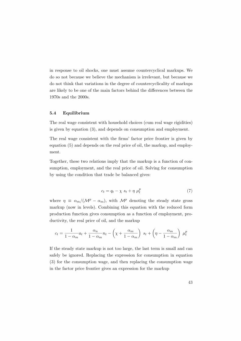
The Macroeconomic Effects Of Oil Price Shocks:Why Are The 2000s So Different From The 1970s?
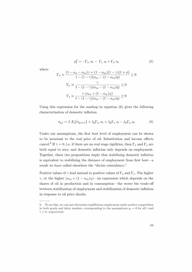
07-011


The Macroeconomic Effects of Oil Price
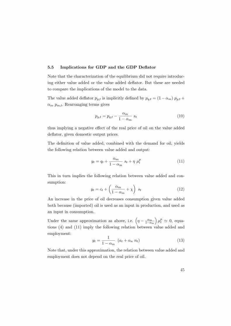
Shocks: Why are the 2000s so different
from the 1970s?∗
Olivier J. Blanchard† Jordi Galı ‡
August 18, 2007
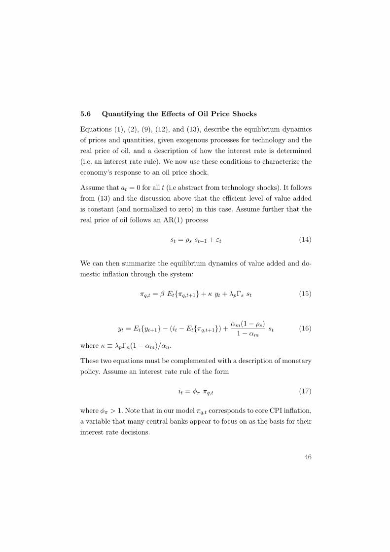
Abstract
We characterize the macroeconomic performance of a set of industrializedeconomies in the aftermath of the oil price shocks of the 1970s and ofthe last decade, focusing on the differences across episodes. We examinefour different hypotheses for the mild effects on inflation and economicactivity of the recent increase in the price of oil: (a) good luck (i.e. lackof concurrent adverse shocks), (b) smaller share of oil in production, (c)more flexible labor markets, and (d) improvements in monetary policy. Weconclude that all four have played an important role.
∗ We are grateful for helpful comments and suggestions to Julio Rotemberg, JohnParsons, Lutz Kilian, Jose de Gregorio, Gauti Eggertson and participants at NBER MEMeeting, the NBER Conference on “International Dimensions of Monetary Policy”, andseminars at CREI-UPF. We thank Davide Debortoli for excellent research assistance,and the NSF and the Banque de France Foundation for financial assistance.† MIT and NBER.‡ CREI, UPF and NBER.
1
Introduction
Since the 1970s, and at least until recently, macroeconomists have viewedchanges in the price of oil as as an important source of economic fluc-tuations, as well as a paradigm of a global shock, likely to affect manyeconomies simultaneously. Such a perception is largely due to the twoepisodes of low growth, high unemployment, and high inflation that char-acterized most industrialized economies in the mid and late 1970s. Con-ventional accounts of those episodes of stagflation blame them on the largeincreases in the price of oil triggered by the Yom Kippur war in 1973, andthe Iranian revolution of 1979, respectively.1
The events of the past decade, however, seem to call into question the rel-evance of oil price changes as a significant source of economic fluctuations.The reason: Since the late 1990s, the global economy has experienced twooil shocks of sign and magnitude comparable to those of the 1970s but, incontrast with the latter episodes, GDP growth and inflation have remainedrelatively stable in much of the industrialized world.
Our goal in this paper is to shed light on the nature of the apparent changesin the macroeconomic effects of oil shocks, as well as on some of its possiblecauses. Disentangling the factors behind those changes is obviously key toassessing the extent to which the episodes of stagflation of the 1970s canreoccur in response to future oils shocks and, if so, to understanding therole that monetary policy can play in order to mitigate their adverse effects.
One plausible hypothesis is that the effects of the increase in the price of oilproper have been similar across episodes, but have coincided in time withlarge shocks of a very different nature (e.g. large rises in other commodityprices in the 1970s, high productivity growth and world demand in the2000s). That coincidence could significantly distort any assessment of the
1. Most undergraduate textbooks make an unambiguous connection between the twooil price hikes of 1973-1974 and 1979-1980 and the period of stagflation that ensued. Seee.g. Mankiw (2007, p. 274).
2
impact of oil shocks based on a simple observation of the movements inaggregate variables around each episode.
In order to evaluate this hypothesis one must isolate the component ofmacroeconomic fluctuations associated with exogenous changes in the priceof oil. To do so, we identify and estimate the effects of an oil price shockusing structural VAR techniques. We report and compare estimates fordifferent sample periods and discuss how they have changed over time. Wefollow two alternative approaches. The first one is based on a large VAR,and allows for a break in the sample in the mid 1980s. The second approachis based on rolling bivariate VARs, including the price of oil and one othervariable at a time. The latter approach allows for a gradual change in theestimated effects of oil price shocks, without imposing a discrete break ina single period.
Two conclusions clearly emerge from this analysis: First, there were indeedother adverse shocks at work in the 1970s; the price of oil explains only partof the stagflation episodes of the 1970s. Second, and importantly, the effectsof a given change in the price of oil have changed substantially over time.Our estimates point to much larger effects of oil price shocks on inflationand activity in the early part of the sample, i.e. the one that includes thetwo oil shock episodes of the 1970s.
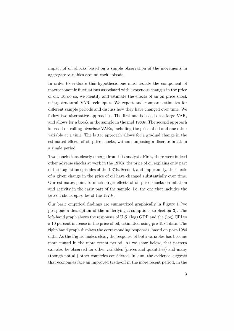
Our basic empirical findings are summarized graphically in Figure 1 (wepostpone a description of the underlying assumptions to Section 3). Theleft-hand graph shows the responses of U.S. (log) GDP and the (log) CPI toa 10 percent increase in the price of oil, estimated using pre-1984 data. Theright-hand graph displays the corresponding responses, based on post-1984data. As the Figure makes clear, the response of both variables has becomemore muted in the more recent period. As we show below, that patterncan also be observed for other variables (prices and quantities) and many(though not all) other countries considered. In sum, the evidence suggeststhat economies face an improved trade-off in the more recent period, in the
3
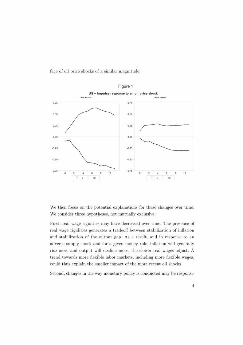
face of oil price shocks of a similar magnitude.
US -- Impulse response to an oil price shock
Pre 1983:04 Post 1984:01
y cpi
0 2 4 6 8 10-0.75
-0.50
-0.25
0.00
0.25
0.50
0.75
y cpi
0 2 4 6 8 10-0.75
-0.50
-0.25
0.00
0.25
0.50
0.75
Figure 1
We then focus on the potential explanations for these changes over time.We consider three hypotheses, not mutually exclusive:
First, real wage rigidities may have decreased over time. The presence ofreal wage rigidities generates a tradeoff between stabilization of inflationand stabilization of the output gap. As a result, and in response to anadverse supply shock and for a given money rule, inflation will generallyrise more and output will decline more, the slower real wages adjust. Atrend towards more flexible labor markets, including more flexible wages,could thus explain the smaller impact of the more recent oil shocks.
Second, changes in the way monetary policy is conducted may be responsi-
4
ble for the differential response of the economy to the oil shocks. In partic-ular, the stronger commitment by central banks to maintaining a low andstable rate of inflation, reflected in the widespread adoption of more or lessexplicit inflation targeting strategies, may have led to an improvement inthe policy tradeoff that make it possible to have a smaller impact of a givenoil price increase on both inflation and output simultaneously.
Third, the share of oil in the economy may have declined sufficiently sincethe 1970s to account for the decrease in the effects of its price changes.Under that hypothesis, changes in the price of oil have increasingly turnedinto a sideshow, with no significant macroeconomic effects (not unlike fluc-tuations in the price of caviar).
To assess the merits of the different hypotheses we proceed in two steps.First, we develop a simple version of the new-Keynesian model where (im-ported) oil is both consumed by households and used as a production inputby firms. The model allows us to examine how the economy’s response toan exogenous change in the price of oil is affected by the degree of real wagerigidities, the nature and credibility of monetary policy, and the share ofoil in production and consumption. We then look for more direct evidencepointing to the relevance and quantitative importance of each of thosehypotheses. We conclude that all three are likely to have played an impor-tant role in explaining the different effects of oil prices during the 1970sand during the last decade.
The paper is organized as follows. Section 1 gives a short summary of howour paper fits in the literature. Section 2 presents basic facts. Section 3presents results from multivariate VARs. Section 4 presents results fromrolling bivariate VARs. Section 5 presents the model. Section 6 uses themodel to analyze the role of real rigidities, credibility in monetary policy,and the oil share. Section 7 concludes.
5

1 Relation to the Literature
Our paper is related to many strands of research.
The first strand is concerned with the effects of oil price shocks on theeconomy. The seminal work in that literature is Bruno and Sachs (1985),who were the first to analyze in depth the effects of oil prices of the 1970s onoutput and inflation in the major industrialized countries. They exploredmany of the themes of our paper, the role of other shocks, the role ofmonetary policy, and the role of wage setting.
On the empirical side, Hamilton showed in a series of contributions (see,in particular, Hamilton (1983, 1996)) that most of U.S. recessions werepreceded by increases in the price of oil, suggesting an essential role for oilprice increases as one of the main cause of recessions. The stability of thisrelation has been challenged by a number of authors, in particular Hooker(1996). Our findings that the effects of the price of oil have changed overtime is consistent with the mixed findings of this line of research.
On the theoretical side, a number of papers have assessed the ability ofstandard models to account for the size and nature of the observed effects ofoil price shocks. Thus, Rotemberg and Woodford (1997) argued that it wasdifficult to explain the sheer size of these effects in the 1970s. They arguedthat something else was going on, namely an endogenous increase in themarkup of firms, leading to a larger decrease in output. Finn (2000) showedthat effects of the relevant size could be generated in a perfectly competitiveRBC model, by allowing for variable capital utilization. Neither mechanismwould seem to account for the depth of the effects of the 1970s and not inthe 2000s. The latter observation motivates our focus on the role of realwage rigidities, and the decline in these rigidities over time, an explanationwe find more convincing than changes in either the behavior of markups orcapacity utilization over time. In following this line, we build on our earlierwork on the implications of real wage rigidities and their interaction with
6
nominal price stickiness (Blanchard and Gali 2007).
A second strand of research related to the present paper deals with thepossible changes over time in the effects of oil shocks. Of course, that strandis in turn related to the literature on the “Great Moderation,” a termused to refer to the decrease in output fluctuations over the last 30 years(e.g., Blanchard and Simon (2001), Stock and Watson (2003)). The latterliterature has tried to assess to what extent the declines in volatility havebeen due to ”good luck” (i.e. smaller shocks) or changes in the economy’sstructure (including policy changes). In that context, some authors haveargued that the stagflations of the 1970s were largely due to factors otherthan oil. Most prominently, Barsky and Kilian (2002) argue that they mayhave been partly caused by exogenous changes in monetary policy, whichcoincided in time with the rise in oil prices. Bernanke, Gertler, and Watson(1997) argue that much of the decline in output and employment was dueto the rise in interest rates, resulting from the Fed’s endogenous responseto the higher inflation induced by the oil shocks.
While our evidence suggests that oil price shocks can only account for afraction of the fluctuations of the 1970s, our findings that the dynamiceffects of oil shocks have decreased considerably over time, combined withthe observation that the oil shocks themselves have been no smaller, isconsistent with the hypothesis of structural change.
We know of four papers which specifically focus, as we do, on the chang-ing impact of oil shocks. Hooker (2002) analyzes empirically the changingweight of oil prices as an explanatory variable in a traditional Phillipscurve specification for the U.S. economy. He finds that pass-through fromoil to prices has become negligible since the early eighties, but cannot findevidence for a significant role of the decline in energy intensity, the dereg-ulation of energy industries, or changes in monetary policy as a factor
7
behind that lower pass-through. De Gregorio, Landerretche, and Neilson(2007) provide a variety of estimates of the degree of pass-through from oilprices to inflation, and its changes over time, for a large set of countries. Inaddition to estimates of Phillips curves along the lines of Hooker (2002),they also provide evidence based on rolling VARs, as we do in the presentpaper, though they use a different specification, and focus exclusively onthe effects on inflation. Their paper also examines a number of potentialexplanations, including a change in the response of the exchange rate (inthe case of non-U.S. countries), and the virtuous effects of being in a lowinflation environment. In two recent papers, developed independently, Her-rera and Pesavento (2007), and Edelstein and Kilian (2007), also documentthe decrease in the effects of oil shocks on a number of aggregate variablesusing a VAR approach. Herrera and Pesavento, following the approach ofBernanke, Gertler and Watson (1997), explore the role of changes in re-sponse of monetary policy to oil shocks in accounting for the more mutedeffects of those shocks in the recent period. Their answer is largely neg-ative: Their findings point to a more stabilizing role of monetary policyin the 1970s relative to the recent period. Edelstein and Kilian focus onchanges in the composition of U.S. automobile production, and the declin-ing importance of the U.S. automobile sector. Given that the decline in theeffects of the price of oil appears to be present in a large number of OECDcountries, this explanation appears perhaps too U.S. specific.
2 Basic Facts
Figure 2 displays the evolution of the price of oil since 1970. More specif-ically, it shows the quarterly average price of a barrel of West Texas In-termediate, measured in U.S. dollars.2 The figure shows how a long spell
2. The description of the stylized facts discussed below is not altered significantly ifone uses alternative oil price measures, such as the PPI index for crude oil (used e.g. by
8
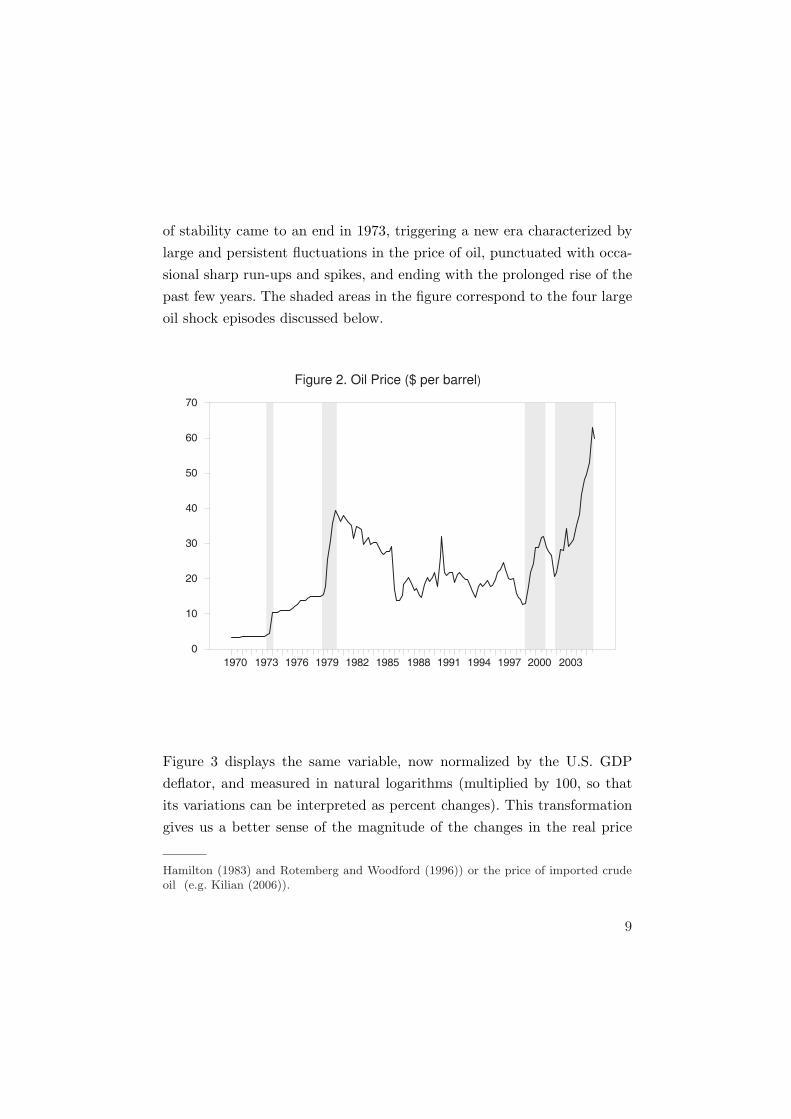
of stability came to an end in 1973, triggering a new era characterized bylarge and persistent fluctuations in the price of oil, punctuated with occa-sional sharp run-ups and spikes, and ending with the prolonged rise of thepast few years. The shaded areas in the figure correspond to the four largeoil shock episodes discussed below.
1970 1973 1976 1979 1982 1985 1988 1991 1994 1997 2000 2003
0
10
20
30
40
50
60
70
Figure 2. Oil Price ($ per barrel)
Figure 3 displays the same variable, now normalized by the U.S. GDPdeflator, and measured in natural logarithms (multiplied by 100, so thatits variations can be interpreted as percent changes). This transformationgives us a better sense of the magnitude of the changes in the real price
Hamilton (1983) and Rotemberg and Woodford (1996)) or the price of imported crudeoil (e.g. Kilian (2006)).
9
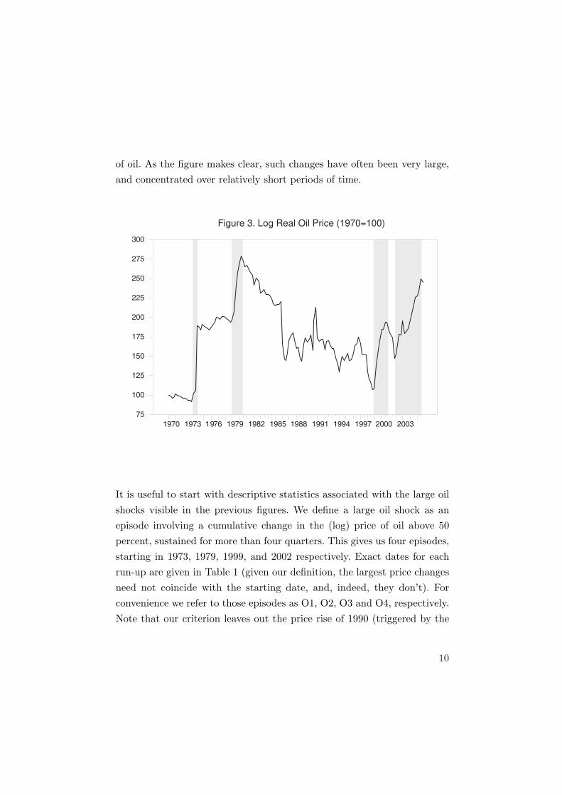
of oil. As the figure makes clear, such changes have often been very large,and concentrated over relatively short periods of time.
1970 1973 1976 1979 1982 1985 1988 1991 1994 1997 2000 2003
75
100
125
150
175
200
225
250
275
300
Figure 3. Log Real Oil Price (1970=100)
It is useful to start with descriptive statistics associated with the large oilshocks visible in the previous figures. We define a large oil shock as anepisode involving a cumulative change in the (log) price of oil above 50percent, sustained for more than four quarters. This gives us four episodes,starting in 1973, 1979, 1999, and 2002 respectively. Exact dates for eachrun-up are given in Table 1 (given our definition, the largest price changesneed not coincide with the starting date, and, indeed, they don’t). Forconvenience we refer to those episodes as O1, O2, O3 and O4, respectively.Note that our criterion leaves out the price rise of 1990 (triggered by the
10
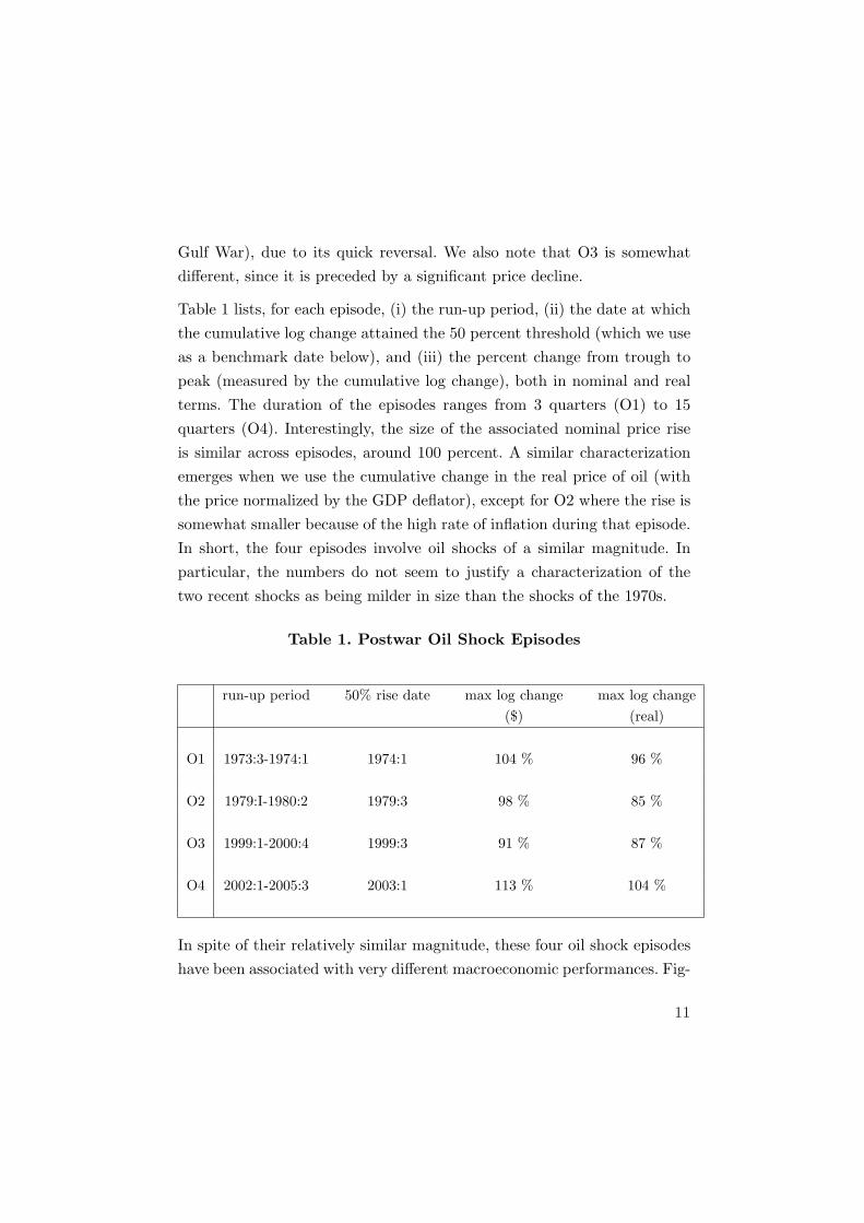
Gulf War), due to its quick reversal. We also note that O3 is somewhatdifferent, since it is preceded by a significant price decline.
Table 1 lists, for each episode, (i) the run-up period, (ii) the date at whichthe cumulative log change attained the 50 percent threshold (which we useas a benchmark date below), and (iii) the percent change from trough topeak (measured by the cumulative log change), both in nominal and realterms. The duration of the episodes ranges from 3 quarters (O1) to 15quarters (O4). Interestingly, the size of the associated nominal price riseis similar across episodes, around 100 percent. A similar characterizationemerges when we use the cumulative change in the real price of oil (withthe price normalized by the GDP deflator), except for O2 where the rise issomewhat smaller because of the high rate of inflation during that episode.In short, the four episodes involve oil shocks of a similar magnitude. Inparticular, the numbers do not seem to justify a characterization of thetwo recent shocks as being milder in size than the shocks of the 1970s.
Table 1. Postwar Oil Shock Episodes
run-up period 50% rise date max log change max log change($) (real)
O1 1973:3-1974:1 1974:1 104 % 96 %
O2 1979:I-1980:2 1979:3 98 % 85 %
O3 1999:1-2000:4 1999:3 91 % 87 %
O4 2002:1-2005:3 2003:1 113 % 104 %
In spite of their relatively similar magnitude, these four oil shock episodeshave been associated with very different macroeconomic performances. Fig-
11

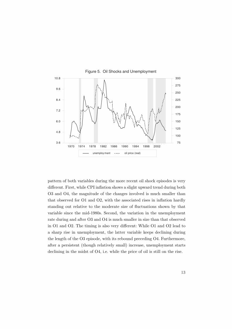
ures 4 and 5, which show respectively the evolution of (annual) CPI infla-tion and the unemployment rate in the U.S. over the period 1970:1-2005:4,provide a visual illustration.
Figure 4. Oil Shocks and CPI Inflation
cpi inf lation oil price (real)
1970 1974 1978 1982 1986 1990 1994 1998 2002
0
2
4
6
8
10
12
14
75
100
125
150
175
200
225
250
275
300
Each figure shows, in addition to the variable displayed, the (log) real priceof oil and the four shaded areas representing our four oil shock episodes.Note that the timing of O1 and O2 coincide with a sharp increase in infla-tion, and mark the beginning of a large rise in the unemployment rate. Ineach case, both inflation and unemployment reached a peak a few quartersafter the peak in oil prices (up to a level of 11.3% and 13.4%, respectively,in the case of inflation, 8.8% and 10.6% for the unemployment rate). The
12
unemploy ment oil price (real)
1970 1974 1978 1982 1986 1990 1994 1998 2002
3.6
4.8
6.0
7.2
8.4
9.6
10.8
75
100
125
150
175
200
225
250
275
300
Figure 5. Oil Shocks and Unemployment
pattern of both variables during the more recent oil shock episodes is verydifferent. First, while CPI inflation shows a slight upward trend during bothO3 and O4, the magnitude of the changes involved is much smaller thanthat observed for O1 and O2, with the associated rises in inflation hardlystanding out relative to the moderate size of fluctuations shown by thatvariable since the mid-1980s. Second, the variation in the unemploymentrate during and after O3 and O4 is much smaller in size than that observedin O1 and O2. The timing is also very different: While O1 and O2 lead toa sharp rise in unemployment, the latter variable keeps declining duringthe length of the O3 episode, with its rebound preceding O4. Furthermore,after a persistent (though relatively small) increase, unemployment startsdeclining in the midst of O4, i.e. while the price of oil is still on the rise.
13

Tables 2 and 3 provide related evidence for each of the G7 countries as wellas for three aggregates (the G7, the euro-12, and the OECD countries).3
More specifically, Table 2 displays, for each country and episode, the aver-age rate of inflation over the 8 quarters following each episode’s benchmarkdate (at which the 50% threshold oil price rise is reached) minus the aver-age rate of inflation over the 8 quarters immediately preceding each run-up.Note that the increase in inflation associated with O1 is typically largerthan the one for O2. The most striking evidence, however, relates to O3and O4, which are typically associated with a change in inflation in theiraftermath of a much smaller size than that following O1 and O2.4 The lasttwo columns, which average the inflation change for O1-O2 and O3-O4,makes the same point in a more dramatic way.
Table 2. Oil Shock Episodes: Change in Inflation
O1 O2 O3 O4 AVG (1,2) AVG (3,4)
Canada 4.7 1.8 2.2 0.5 3.3 1.4Germany 0.1 2.6 1.1 -0.2 1.4 0.4France 5.4 3.1 1.3 0.5 4.2 0.9U.K. 10.2 4.3 0.0 0.5 7.3 0.3Italy 7.7 5.6 1.0 -0.1 6.6 0.4Japan 7.9 1.0 -1.7 0.9 4.4 -0.4U.S. 4.9 4.0 1.7 -0.2 4.5 0.7G7 4.8 1.9 0.3 0.0 3.3 0.2Euro12 4.3 2.7 1.3 -0.5 3.5 0.4OECD 4.9 1.8 0.1 -0.5 3.4 -0.2
3. We use quarterly data from OECD’s Economic Outlook Database. For the purposeof this exercise, inflation is the annualized quarter-to-quarter rate of change in the CPI.4. Even for Canada and Germany, the largest change in inflation occurs in either O1or O2.
14
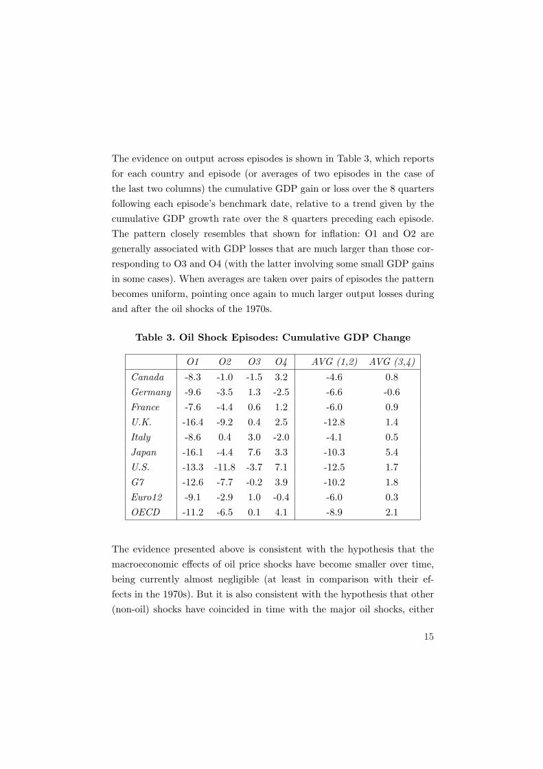
The evidence on output across episodes is shown in Table 3, which reportsfor each country and episode (or averages of two episodes in the case ofthe last two columns) the cumulative GDP gain or loss over the 8 quartersfollowing each episode’s benchmark date, relative to a trend given by thecumulative GDP growth rate over the 8 quarters preceding each episode.The pattern closely resembles that shown for inflation: O1 and O2 aregenerally associated with GDP losses that are much larger than those cor-responding to O3 and O4 (with the latter involving some small GDP gainsin some cases). When averages are taken over pairs of episodes the patternbecomes uniform, pointing once again to much larger output losses duringand after the oil shocks of the 1970s.
Table 3. Oil Shock Episodes: Cumulative GDP Change
O1 O2 O3 O4 AVG (1,2) AVG (3,4)
Canada -8.3 -1.0 -1.5 3.2 -4.6 0.8Germany -9.6 -3.5 1.3 -2.5 -6.6 -0.6France -7.6 -4.4 0.6 1.2 -6.0 0.9U.K. -16.4 -9.2 0.4 2.5 -12.8 1.4Italy -8.6 0.4 3.0 -2.0 -4.1 0.5Japan -16.1 -4.4 7.6 3.3 -10.3 5.4U.S. -13.3 -11.8 -3.7 7.1 -12.5 1.7G7 -12.6 -7.7 -0.2 3.9 -10.2 1.8Euro12 -9.1 -2.9 1.0 -0.4 -6.0 0.3OECD -11.2 -6.5 0.1 4.1 -8.9 2.1
The evidence presented above is consistent with the hypothesis that themacroeconomic effects of oil price shocks have become smaller over time,being currently almost negligible (at least in comparison with their ef-fects in the 1970s). But it is also consistent with the hypothesis that other(non-oil) shocks have coincided in time with the major oil shocks, either
15
reinforcing the adverse effects of the latter in the 1970s, or dampening themduring the more recent episodes. In order to sort out those possibilities weturn next to a more structured analysis of the co-movements between oilprices and other variables.
3 Estimating the Effects of Oil Price Shocks using
Structural VARs
In this section we provide more structural evidence on the macroeconomiceffects of oil price shocks, and changes over time in the nature and size ofthose effects. We provide evidence for the United States, France, Germany,the United Kingdom, Italy, and Japan, using a 6-variable VAR. In the nextsection we turn to a more detailed analysis of the U.S. evidence, using abattery of rolling bivariate VARs.
Our baseline VAR makes use of data on the nominal price of oil (in dollars),three inflation measures (CPI, GDP deflator, and wages) and two quantities(GDP and employment). By using a multivariate specification, we allowfor a variety of shocks in addition to the oil shock that is our focus ofinterest. We identify oil shocks by assuming that unexpected variationsin the nominal price of oil are exogenous relative to the contemporaneousvalues of the remaining macroeconomic variables included in the VAR.In other words, we take the oil shock to correspond to the reduced forminnovation to the (log) nominal oil price, measured in U.S. dollars.
This identification assumption will clearly be incorrect if economic devel-opments in the country under consideration affect the world price of oilcontemporaneously. This may be either because the economy under con-sideration is large, or because developments in the country are correlatedwith world developments. For example, Rotemberg and Woodford (1996),who rely on the same identification assumption as we do when studying
16
the effects of oil shocks on the U.S. economy, restrict their sample periodto end in 1980 on the grounds that variations in the price of oil may havea significant endogenous component after that date. We have thereforeexplored an alternative assumption, namely, letting the price of oil reactcontemporaneously to current developments in the two quantity variables(output, and employment), while assuming that quantity variables do notreact contemporaneously to the price of oil. Because the contemporaneouscorrelations between quarterly quantity and oil price innovations are small,the results are nearly identical, and we do not report them in the text.
Another approach would be to use, either in addition or in substitution tothe oil price, a more exogenous variable to proxy for oil shocks. This is theapproach followed by Kilian (2007), who constructs and uses a proxy forunexpected movements in global oil production. What matters, however,to any given country is not the level of global oil production, but the priceat which firms and households can purchase oil, which in turn depends alsoon world demand for oil. Thus, if the price of oil rises as a result of, say,higher Chinese demand, this is just like an exogenous oil supply shock forthe remaining countries. This is indeed why we are fairly confident in ouridentification approach: The large residuals in our oil price series are clearlyassociated either with identifiable episodes of large supply disruptions or,in the more recent past, with increases in emerging countries’ demand.These observations largely drive our estimates and our impulse responsefunctions.
For each of the six countries, we estimate a VAR containing six variables:the dollar price of oil (expressed in log differences), CPI inflation, GDPdeflator inflation, wage inflation, and the log changes in GDP and employ-ment.5 We use the dollar price of oil rather than the real price of oil, to
5. For the United States we use non-farm business hours instead of employment, and thewage refers to non-farm business compensation per hour. For simplicity we use the termemployment to refer to both hours (in the case of the United States) and employmentproper (for the remaining countries).
17
avoid dividing by an endogenous variable, the GDP deflator. For the samereason we do not convert the price of oil into domestic currency for non-UScountries. For the United States, the data are taken from the USECONdatabase, and cover the sample period 1960:1-2005:4. For the remainingcountries, the data are drawn from OECD’s Economic Outlook database,with the sample period being 1970:1-2005:4. Our three inflation measuresare quarter-to-quarter, expressed in annualized terms. Each equation inour VAR includes four lags of the six variables above, a constant term anda quadratic trend fitted measure of productivity growth.
Some of the oil price changes, and by implication, some of the residuals inthe price of oil equation, are extremely large. The change in the price ofoil for 1974:1, for example, is equal to eight times its standard deviationover the sample. Such large changes are likely to lead to small sample biaswhen estimating the oil price equation: The best OLS fit is achieved byreducing the size of these particular residuals, thus by spuriously linkingthese very large realizations to movements in current or past values of theother variables in the regression. This in turn overstates the endogenouscomponent of the price of oil, and understates the size of the true residuals.We deal with this issue by estimating the oil price equation using a samplewhich excludes all oil price changes larger than three standard deviations.(These large changes in oil prices are clearly essential in giving us preciseestimates of the effects of oil prices on other variables. Thus, we use thecomplete sample when estimating the other equations.)
3.1 Impulse Responses
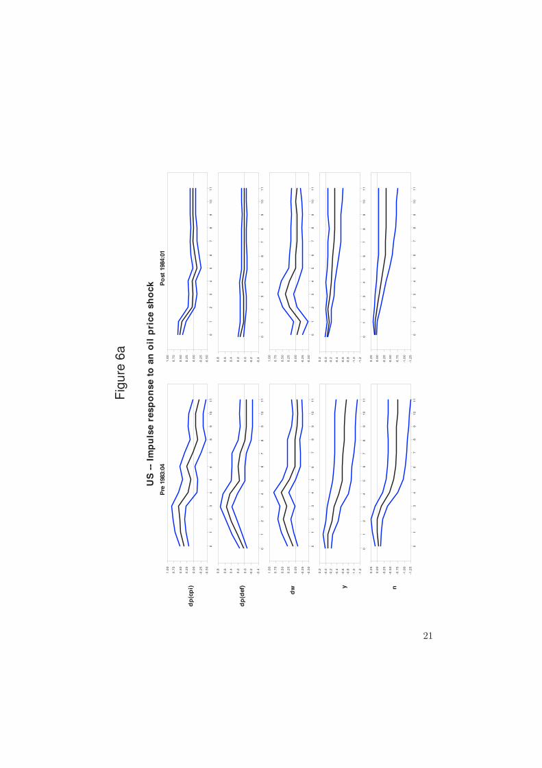
Figures 6a-6f display the estimated impulse response functions (IRFs) forthe different variables of interest to an oil price shock where, as discussedabove, the latter is identified as the innovation in the oil price equation.Estimates are reported for two different sample periods: 1970:1-1983:4 and1984:1-2006:4. The break date chosen corresponds roughly to the beginning
18
of the Great Moderation in the United States, as identified by severalauthors (e.g. McConnell and Perez-Quiros (2000). Note that each subperiodcontains two of the four large oil shock episodes identified in the previoussection.
One-standard-deviation confidence intervals, obtained using a Monte Carloprocedure, are shown on both sides of the point estimates. The estimatedresponses of GDP and employment are accumulated and shown in levels.The size of the shock is normalized so that it raises the price of oil by 10percent on impact. This roughly corresponds to the estimated standarddeviations of oil price innovations for the two subsamples, which are verysimilar.6 In all cases, the real price of oil shows a near-random walk response(not shown here), i.e. it jumps on impact, and then stays around a newplateau.
The estimates for the United States, shown in Figure 6a, fit pretty wellthe conventional wisdom about the effects of a rise in oil prices. (Figure 1,presented in the introduction, corresponds to Figure 6a, with the resultsfor the CPI shown in levels rather than rates of change.) For the pre-1984 period, CPI inflation shifts up immediately, and remains positive fora protracted period. The response of GDP inflation and wage inflation issimilar, though more gradual. Output and employment decline persistently,albeit with a lag. Most relevant for our purposes, the responses of thesame variables in the post-1984 period are considerably more muted, thussuggesting a weaker impact of oil price shocks on the economy. The onlyexception to this pattern is given by CPI inflation, whose response onimpact is very similar across periods (though its persistence is smaller inthe second period). This may not be surprising since part of the increasein oil prices is reflected mechanically in the oil component of the CPI.
6. The estimated standard deviation of oil price innovations is 9.4 percent in the pre-1984 period, 12.4 percent in the post-84 period.
19
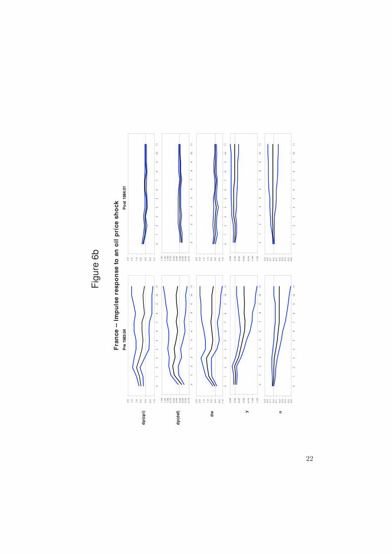
The estimates for France and the United Kingdom show a pattern very sim-ilar to that of the United States. In the case of France, the contrast betweenthe early and the late periods is particularly strong, both in terms of thesize and the persistence of the effects, and for both prices and quantities. Inthe case of the United Kingdom, the response of inflation variables is almostnon-existent in the latter period though, in contrast with France, there issome evidence of a decline in output and employment (albeit smaller thanin the first sample period).
Some of the estimated responses for Germany and Italy fit conventionalwisdom less well. The inflation measures in Germany hardly change inresponse to the rise in oil prices in either period, though the impact onoutput and employment is more adverse in the pre-1984 period. This isconsistent with a stronger anti-inflationary stance of the Bundesbank, rel-ative to other central banks. The slight increase in employment and outputin the post-1984 period goes against conventional wisdom. In the case ofItaly, there is barely any employment response in the pre-1984 period. Still,for both countries the sign of most of the responses accord with conven-tional wisdom, and the responses are smaller in the post-1984 period.
The story is different for Japan. The sign of many of the responses to therise in oil prices is often at odds with standard priors. Also, the uncertaintyof the estimates is much larger, as reflected in the wider bands. The effecton inflation is weak and does not have a clear sign in either period. Thereis a (slight) rise in output in both periods, and of employment in the post-1984 period.
In short, except for Japan (and to some extent, for Germany), most of theresponses fit conventional wisdom rather well: An increase in the price ofoil leads to more wage and price inflation, and to a decrease in employmentand output for some time. In all cases, however, the effects on both inflationand activity are considerably weaker in the second subsample than in thefirst.
20
US
--
Imp
uls
e r
esp
on
se
to
an
oil
pri
ce s
ho
ck
dp
(cp
i)
dp
(def)
dw y n
Pre
1983:0
4P
ost
1984:0
1
01
23
45
67
89
10
11
-0.5
0
-0.2
5
0.0
0
0.2
5
0.5
0
0.7
5
1.0
0
01
23
45
67
89
10
11
-0.4
-0.2
0.0
0.2
0.4
0.6
0.8
01
23
45
67
89
10
11
-0.5
0
-0.2
5
0.0
0
0.2
5
0.5
0
0.7
5
1.0
0
01
23
45
67
89
10
11
-1.2
-1.0
-0.8
-0.6
-0.4
-0.2
-0.0
0.2
01
23
45
67
89
10
11
-1.2
5
-1.0
0
-0.7
5
-0.5
0
-0.2
5
0.0
0
0.2
5
01
23
45
67
89
10
11
-0.5
0
-0.2
5
0.0
0
0.2
5
0.5
0
0.7
5
1.0
0
01
23
45
67
89
10
11
-0.4
-0.2
0.0
0.2
0.4
0.6
0.8
01
23
45
67
89
10
11
-0.5
0
-0.2
5
0.0
0
0.2
5
0.5
0
0.7
5
1.0
0
01
23
45
67
89
10
11
-1.2
-1.0
-0.8
-0.6
-0.4
-0.2
-0.0
0.2
01
23
45
67
89
10
11
-1.2
5
-1.0
0
-0.7
5
-0.5
0
-0.2
5
0.0
0
0.2
5
Fig
ure
6a
21
Fra
nce -
- Im
pu
lse r
esp
on
se t
o a
n o
il p
ric
e s
ho
ck
dp
(cp
i)
dp
(def)
dw y n
Pre
1983:0
4P
ost
1984:0
1
01
23
45
67
89
10
11
-1.0
-0.5
0.0
0.5
1.0
1.5
2.0
01
23
45
67
89
10
11
-0.7
5
-0.5
0
-0.2
5
0.0
0
0.2
5
0.5
0
0.7
5
1.0
0
1.2
5
1.5
0
01
23
45
67
89
10
11
-1.0
-0.5
0.0
0.5
1.0
1.5
2.0
2.5
01
23
45
67
89
10
11
-1.2
5
-1.0
0
-0.7
5
-0.5
0
-0.2
5
0.0
0
0.2
5
01
23
45
67
89
10
11
-0.6
-0.5
-0.4
-0.3
-0.2
-0.1
-0.0
0.1
0.2
0.3
01
23
45
67
89
10
11
-1.0
-0.5
0.0
0.5
1.0
1.5
2.0
01
23
45
67
89
10
11
-0.7
5
-0.5
0
-0.2
5
0.0
0
0.2
5
0.5
0
0.7
5
1.0
0
1.2
5
1.5
0
01
23
45
67
89
10
11
-1.0
-0.5
0.0
0.5
1.0
1.5
2.0
2.5
01
23
45
67
89
10
11
-1.2
5
-1.0
0
-0.7
5
-0.5
0
-0.2
5
0.0
0
0.2
5
01
23
45
67
89
10
11
-0.6
-0.5
-0.4
-0.3
-0.2
-0.1
-0.0
0.1
0.2
0.3
Fig
ure
6b
22
UK
--
Imp
uls
e r
es
po
nse
to
an
oil
pri
ce
sh
ock
dp
(cp
i)
dp
(def)
dw y n
Pre
1983:0
4P
ost
1984:0
1
01
23
45
67
89
10
11
-3-2-1012345
01
23
45
67
89
10
11
-6-4-20246
01
23
45
67
89
10
11
-4-3-2-101234
01
23
45
67
89
10
11
-3.5
-3.0
-2.5
-2.0
-1.5
-1.0
-0.5
0.0
0.5
01
23
45
67
89
10
11
-1.2
5
-1.0
0
-0.7
5
-0.5
0
-0.2
5
0.0
0
0.2
5
01
23
45
67
89
10
11
-3-2-1012345
01
23
45
67
89
10
11
-6-4-20246
01
23
45
67
89
10
11
-4-3-2-101234
01
23
45
67
89
10
11
-3.5
-3.0
-2.5
-2.0
-1.5
-1.0
-0.5
0.0
0.5
01
23
45
67
89
10
11
-1.2
5
-1.0
0
-0.7
5
-0.5
0
-0.2
5
0.0
0
0.2
5
01
23
45
67
89
10
11
-3-2-1012345
01
23
45
67
89
10
11
-6-4-20246
01
23
45
67
89
10
11
-4-3-2-101234
01
23
45
67
89
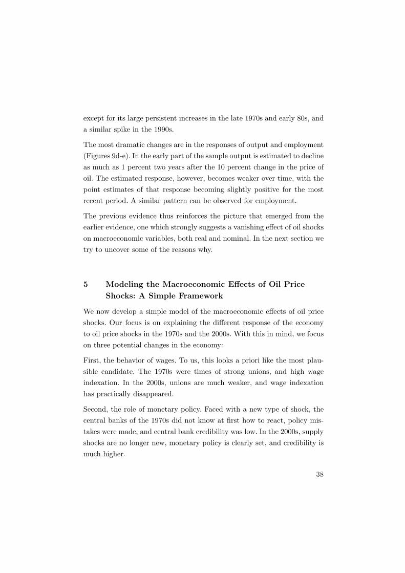
10
11
-3.5
-3.0
-2.5
-2.0
-1.5
-1.0
-0.5
0.0
0.5
01
23
45
67
89
10
11
-1.2
5
-1.0
0
-0.7
5
-0.5
0
-0.2
5
0.0
0
0.2
5
01
23
45
67
89
10
11
-3-2-1012345
01
23
45
67
89
10
11
-6-4-20246
01
23
45
67
89
10
11
-4-3-2-101234
01
23
45
67
89
10
11
-3.5
-3.0
-2.5
-2.0
-1.5
-1.0
-0.5
0.0
0.5
01
23
45
67
89
10
11
-1.2
5
-1.0
0
-0.7
5
-0.5
0
-0.2
5
0.0
0
0.2
5
Fig
ure
6c
23
Germ
an
y -
- Im
pu
lse r
esp
on
se t
o a
n o
il p
ric
e s
ho
ck
dp
(cp
i)
dp
(def)
dw y n
Pre
1983:0
4P
ost
1984:0
1
01
23
45
67
89
10
11
-1.0
-0.8
-0.6
-0.4
-0.2
-0.0
0.2
0.4
0.6
01
23
45
67
89
10
11
-0.8
-0.6
-0.4
-0.2
-0.0
0.2
0.4
0.6
0.8
01
23
45
67
89
10
11
-0.8
-0.6
-0.4
-0.2
-0.0
0.2
0.4
0.6
0.8
01
23
45
67
89
10
11
-0.7
5
-0.5
0
-0.2
5
0.0
0
0.2
5
0.5
0
0.7
5
01
23
45
67
89
10
11
-0.5
-0.4
-0.3
-0.2
-0.1
-0.0
0.1
0.2
0.3
0.4
01
23
45
67
89
10
11
-1.0
-0.8
-0.6
-0.4
-0.2
-0.0
0.2
0.4
0.6
01
23
45
67
89
10
11
-0.8
-0.6
-0.4
-0.2
-0.0
0.2
0.4
0.6
0.8
01
23
45
67
89
10
11
-0.8
-0.6
-0.4
-0.2
-0.0
0.2
0.4
0.6
0.8
01
23
45
67
89
10
11
-0.7
5
-0.5
0
-0.2
5
0.0
0
0.2
5
0.5
0
0.7
5
01
23
45
67
89
10
11
-0.5
-0.4
-0.3
-0.2
-0.1
-0.0
0.1
0.2
0.3
0.4
Fig
ure
6d
24
Italy
--
Imp
uls
e r
esp
on
se t
o a
n o
il p
rice s
ho
ck
dp
(cp
i)
dp
(def)
dw y n
Pre
1983:0
4P
ost
1984:0
1
01
23
45
67
89
10
11
-3-2-10123
01
23
45
67
89
10
11
-4-202468
01
23
45
67
89
10
11
-3.2
-2.4
-1.6
-0.8
-0.0
0.8
1.6
2.4
3.2
01
23
45
67
89
10
11
-5-4-3-2-101
01
23
45
67
89
10
11
-1.2
-1.0
-0.8
-0.6
-0.4
-0.2
-0.0
0.2
0.4
0.6
01
23
45
67
89
10
11
-3-2-10123
01
23
45
67
89
10
11
-4-202468
01
23
45
67
89
10
11
-3.2
-2.4
-1.6
-0.8
-0.0
0.8
1.6
2.4
3.2
01
23
45
67
89
10
11
-5-4-3-2-101
01
23
45
67
89
10
11
-1.2
-1.0
-0.8
-0.6
-0.4
-0.2
-0.0
0.2
0.4
0.6
Fig
ure
6e
25
Jap
an
--
Imp
uls
e r
esp
on
se t
o a
n o
il p
rice s
ho
ck
dp
(cp
i)
dp
(def)
dw y n
Pre
1983:0
4P
ost
1984:0
1
01
23
45
67
89
10
11
-6-4-202468
01
23
45
67
89
10
11
-6.4
-4.8
-3.2
-1.6
-0.0
1.6
3.2
4.8
01
23
45
67
89
10
11
-10-8-6-4-2024
01
23
45
67
89
10
11
-0.9
0.0
0.9
1.8
2.7
3.6
4.5
5.4
01
23
45
67
89
10
11
-1.5
0
-1.2
5
-1.0
0
-0.7
5
-0.5
0
-0.2
5
0.0
0
0.2
5
0.5
0
0.7
5
01
23
45
67
89
10
11
-6-4-202468
01
23
45
67
89
10
11
-6.4
-4.8
-3.2
-1.6
-0.0
1.6
3.2
4.8
01
23
45
67
89
10
11
-10-8-6-4-2024
01
23
45
67
89
10
11
-0.9
0.0
0.9
1.8
2.7
3.6
4.5
5.4
01
23
45
67
89
10
11
-1.5
0
-1.2
5
-1.0
0
-0.7
5
-0.5
0
-0.2
5
0.0
0
0.2
5
0.5
0
0.7
5
Fig
ure
6f
26
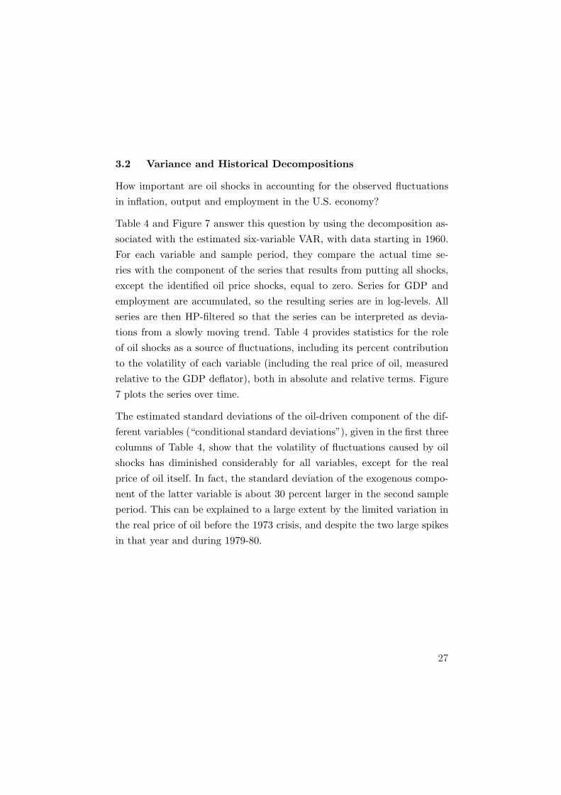
3.2 Variance and Historical Decompositions
How important are oil shocks in accounting for the observed fluctuationsin inflation, output and employment in the U.S. economy?
Table 4 and Figure 7 answer this question by using the decomposition as-sociated with the estimated six-variable VAR, with data starting in 1960.For each variable and sample period, they compare the actual time se-ries with the component of the series that results from putting all shocks,except the identified oil price shocks, equal to zero. Series for GDP andemployment are accumulated, so the resulting series are in log-levels. Allseries are then HP-filtered so that the series can be interpreted as devia-tions from a slowly moving trend. Table 4 provides statistics for the roleof oil shocks as a source of fluctuations, including its percent contributionto the volatility of each variable (including the real price of oil, measuredrelative to the GDP deflator), both in absolute and relative terms. Figure7 plots the series over time.
The estimated standard deviations of the oil-driven component of the dif-ferent variables (“conditional standard deviations”), given in the first threecolumns of Table 4, show that the volatility of fluctuations caused by oilshocks has diminished considerably for all variables, except for the realprice of oil itself. In fact, the standard deviation of the exogenous compo-nent of the latter variable is about 30 percent larger in the second sampleperiod. This can be explained to a large extent by the limited variation inthe real price of oil before the 1973 crisis, and despite the two large spikesin that year and during 1979-80.
27
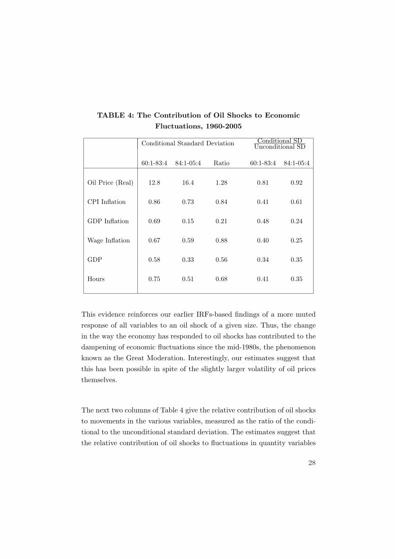
TABLE 4: The Contribution of Oil Shocks to Economic
Fluctuations, 1960-2005
Conditional Standard Deviation Conditional SDUnconditional SD
60:1-83:4 84:1-05:4 Ratio 60:1-83:4 84:1-05:4
Oil Price (Real) 12.8 16.4 1.28 0.81 0.92
CPI Inflation 0.86 0.73 0.84 0.41 0.61
GDP Inflation 0.69 0.15 0.21 0.48 0.24
Wage Inflation 0.67 0.59 0.88 0.40 0.25
GDP 0.58 0.33 0.56 0.34 0.35
Hours 0.75 0.51 0.68 0.41 0.35
This evidence reinforces our earlier IRFs-based findings of a more mutedresponse of all variables to an oil shock of a given size. Thus, the changein the way the economy has responded to oil shocks has contributed to thedampening of economic fluctuations since the mid-1980s, the phenomenonknown as the Great Moderation. Interestingly, our estimates suggest thatthis has been possible in spite of the slightly larger volatility of oil pricesthemselves.
The next two columns of Table 4 give the relative contribution of oil shocksto movements in the various variables, measured as the ratio of the condi-tional to the unconditional standard deviation. The estimates suggest thatthe relative contribution of oil shocks to fluctuations in quantity variables
28
US -- Historical decomposition
dp(cpi)
dp(def)
dw
y
n
Pre 1983:04 Post 1984:01
1961 1963 1965 1967 1969 1971 1973 1975 1977 1979 1981 1983
-6.4
-4.8
-3.2
-1.6
-0.0
1.6
3.2
4.8
6.4
1961 1963 1965 1967 1969 1971 1973 1975 1977 1979 1981 1983
-4
-3
-2
-1
0
1
2
3
4
5
1961 1963 1965 196 7 196 9 197 1 197 3 197 5 197 7 197 9 198 1 198 3
-5.0
-2.5
0.0
2.5
5.0
7.5
10.0
1961 1963 1965 1967 1969 1971 1973 1975 1977 1979 1981 1983
-4
-3
-2
-1
0
1
2
3
4
1961 1963 1965 1967 1969 1971 1973 1975 1977 1979 1981 1983
-5
-4
-3
-2
-1
0
1
2
3
4
1985 1987 1989 1991 1993 1995 1997 1999 2001 2003 2005
-6.4
-4.8
-3.2
-1.6
-0.0
1.6
3.2
4.8
6.4
1985 1987 1989 1991 1993 1995 1997 1999 2001 2003 2005
-4
-3
-2
-1
0
1
2
3
4
5
1985 1987 1989 1991 1993 1995 1997 1999 2001 2003 2005
-5 .0
-2 .5
0.0
2.5
5.0
7.5
10.0
1985 1987 1989 1991 1993 1995 1997 1999 2001 2003 2005
-4
-3
-2
-1
0
1
2
3
4
1985 1987 1989 1991 1993 1995 1997 1999 2001 2003 2005
-5
-4
-3
-2
-1
0
1
2
3
4
Figure 7. The Role of Oil Price Shocks
(GDP and employment) has remained roughly unchanged over time, ataround 1/3. In the case of wage inflation and GDP deflator inflation, thecontribution of oil shocks has declined to 1/4 in both cases, from a levelclose to 1/2. In contrast, the contribution of oil shocks to CPI inflation hasincreased in the recent period. Note that this is consistent with a relativelystable core CPI, with oil price changes being passed through to the energycomponent of the CPI, and accounting for, according to our estimates, asmuch as sixty percent of the fluctuations in overall CPI inflation.
Figure 7 allows us to focus on the contribution of oil prices to the 1973-1974and 1979-1981 episodes. It shows the substantial but non-exclusive role ofexogenous oil shocks during each of the two episodes. In particular, whilefor our three inflation variables the oil price shocks seem to have accountedfor the bulk of the increases in 73-75 and 79-81, no more than a half of
29

the observed decline in employment and output during those episodes canbe attributed to the oil shocks themselves. Thus, our findings suggest thatother shocks played an important role in triggering those episodes.
US -- Historical decomposition
dp(cpi)
dp(def)
dw
y
n
Pre 1983:04 Post 1984:01
1961 1963 1965 1967 1969 1971 1973 1975 1977 1979 1981 1983
-6.4
-4.8
-3.2
-1.6
-0.0
1 .6
3 .2
4 .8
6 .4
1961 1963 1965 1967 1969 1971 1973 1975 1977 1979 1981 1983
-4
-3
-2
-1
0
1
2
3
4
5
1961 1963 1965 196 7 196 9 197 1 197 3 197 5 197 7 197 9 198 1 198 3
-5.0
-2.5
0.0
2.5
5.0
7.5
10.0
1961 1963 1965 1967 1969 1971 1973 1975 1977 1979 1981 1983
-4
-3
-2
-1
0
1
2
3
4
1961 1963 1965 1967 1969 1971 1973 1975 1977 1979 1981 1983
-5
-4
-3
-2
-1
0
1
2
3
4
1985 1987 1989 1991 1993 1995 1997 1999 2001 2003 2005
-6.4
-4.8
-3.2
-1.6
-0.0
1.6
3.2
4.8
6.4
1985 1987 1989 1991 1993 1995 1997 1999 2001 2003 2005
-4
-3
-2
-1
0
1
2
3
4
5
1985 1987 1989 1991 1993 1995 1997 1999 2001 2003 2005
-5.0
-2.5
0.0
2.5
5.0
7.5
10.0
1985 1987 1989 1991 1993 1995 1997 1999 2001 2003 2005
-4
-3
-2
-1
0
1
2
3
4
1985 1987 1989 1991 1993 1995 1997 1999 2001 2003 2005
-5
-4
-3
-2
-1
0
1
2
3
4
Figure 8. The Role of Shocks to Crude Materials Prices
Within our 6-variable VAR, our partial identification approach does notallow us to determine what those additional underlying shocks may havebeen. Yet, when we replace the price of oil by the broader PPI index forcrude materials in our six-variable VAR, the estimates of GDP and em-ployment driven by exogenous shocks to that broader price index trackmore closely the movements of the actual time series themselves in thepre-1984 period, including the two large oil shock episodes contained inthat period, as shown in Figure 8. In particular those shocks account formore than half the fluctuations in all variables over the pre-1984 period.
30
On the other hand, such broader supply shocks play a very limited role inaccounting for the fluctuations in output and employment in the post-1984period (though a more important one in accounting for variations in CPIinflation, in a way consistent with earlier evidence).
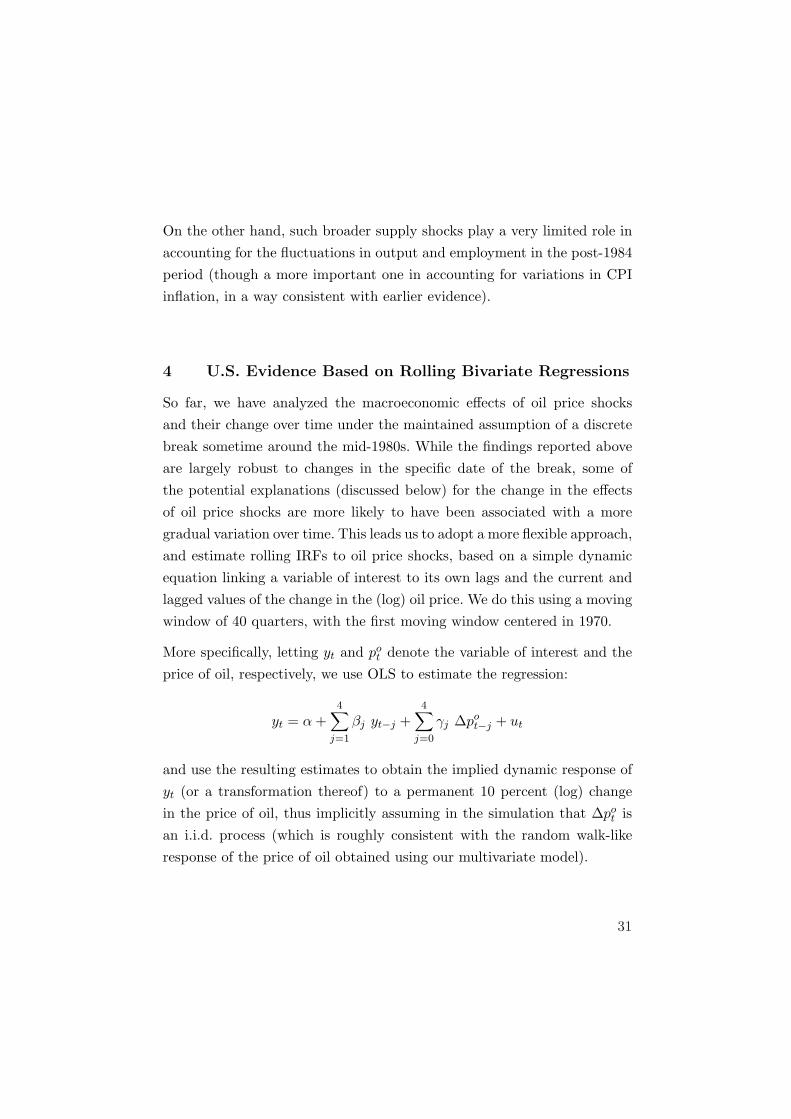
4 U.S. Evidence Based on Rolling Bivariate Regressions
So far, we have analyzed the macroeconomic effects of oil price shocksand their change over time under the maintained assumption of a discretebreak sometime around the mid-1980s. While the findings reported aboveare largely robust to changes in the specific date of the break, some ofthe potential explanations (discussed below) for the change in the effectsof oil price shocks are more likely to have been associated with a moregradual variation over time. This leads us to adopt a more flexible approach,and estimate rolling IRFs to oil price shocks, based on a simple dynamicequation linking a variable of interest to its own lags and the current andlagged values of the change in the (log) oil price. We do this using a movingwindow of 40 quarters, with the first moving window centered in 1970.
More specifically, letting yt and pot denote the variable of interest and the
price of oil, respectively, we use OLS to estimate the regression:
yt = α +4∑
j=1
βj yt−j +4∑
j=0
γj ∆pot−j + ut
and use the resulting estimates to obtain the implied dynamic response ofyt (or a transformation thereof) to a permanent 10 percent (log) changein the price of oil, thus implicitly assuming in the simulation that ∆po
t isan i.i.d. process (which is roughly consistent with the random walk-likeresponse of the price of oil obtained using our multivariate model).
31
Relative to the multivariate model analyzed in the previous section, correctidentification of oil price shocks is obviously more doubtful in the presentbivariate model, given the lower dimension specification of the economy’sdynamics. This shortcoming must be traded-off with the possibility of es-timating the VAR with much shorter samples and, hence, being able toobtain our rolling IRFs. In order to check the consistency with our earlierresults, we first computed the average IRFs across moving windows withineach of the subperiods considered earlier (pre-1984 and post-1984), andfound the estimated IRFs (not shown) to be very similar to the ones ob-tained earlier. In particular, both the inflation variables, as well as outputand employment, show a more muted response in the more recent period.
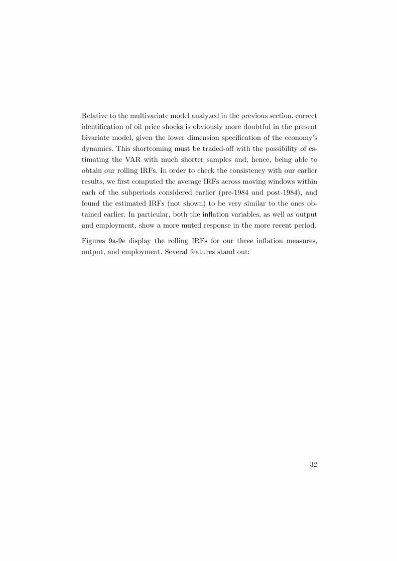
Figures 9a-9e display the rolling IRFs for our three inflation measures,output, and employment. Several features stand out:
32
2
4
6
8
10
12 1970
1975
1980
1985
1990
1995
-0.2
0
0.2
0.4
0.6
0.8
1
1.2
1.4
Period
Response of CPI Inflation
Quarters after shock
Figure 9a
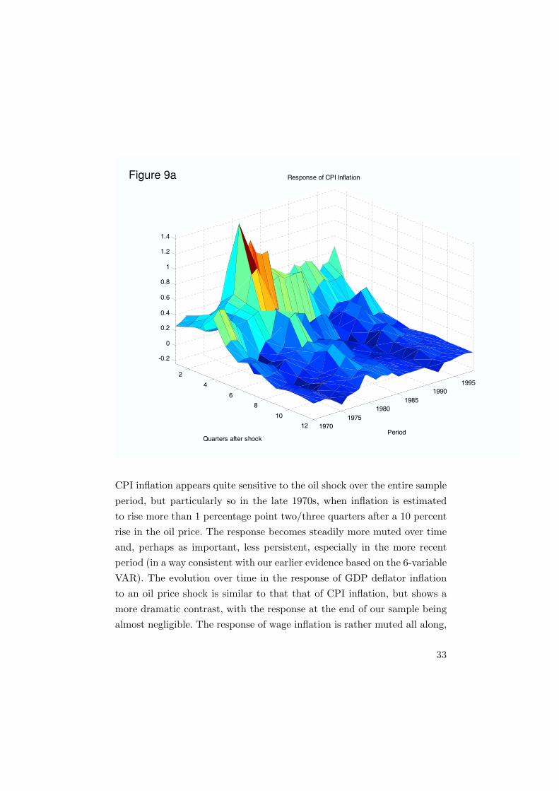
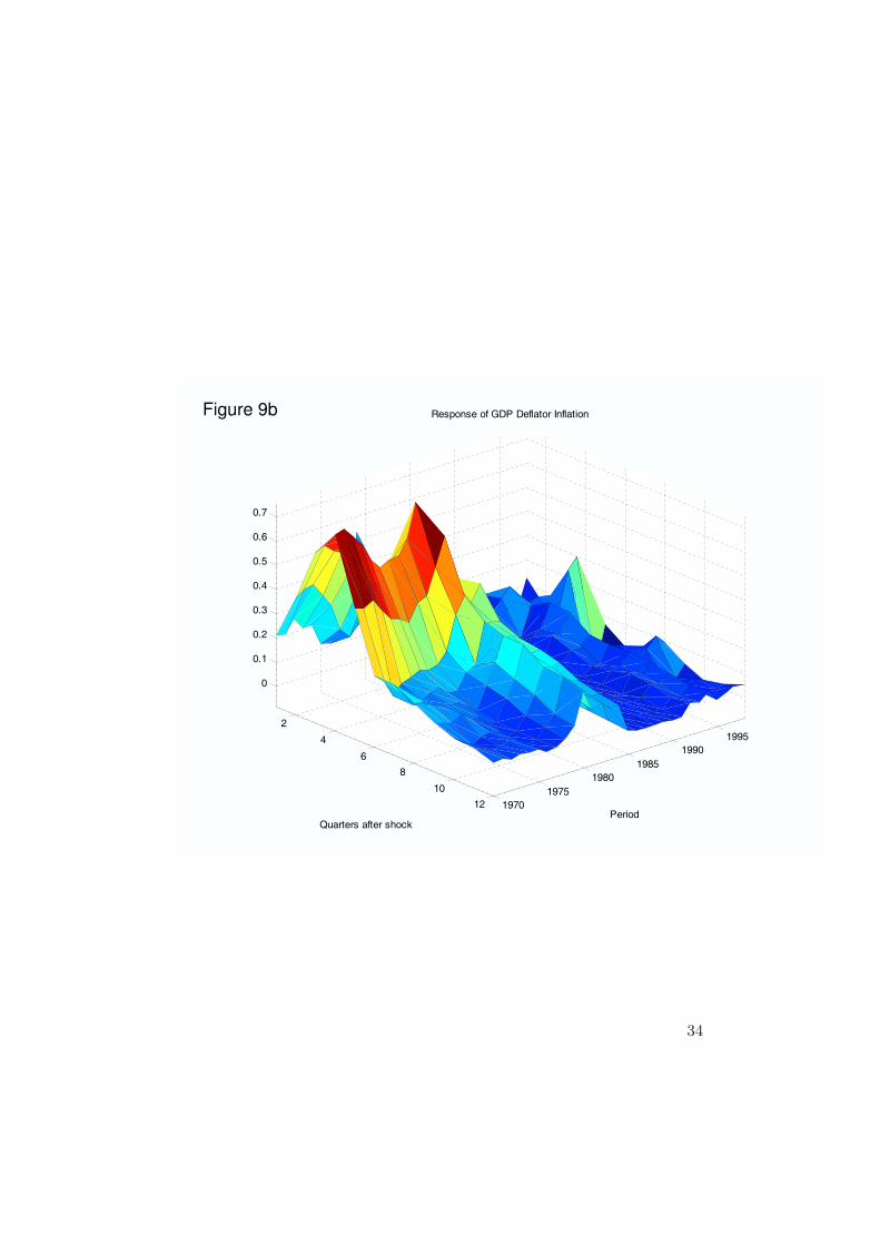
CPI inflation appears quite sensitive to the oil shock over the entire sampleperiod, but particularly so in the late 1970s, when inflation is estimatedto rise more than 1 percentage point two/three quarters after a 10 percentrise in the oil price. The response becomes steadily more muted over timeand, perhaps as important, less persistent, especially in the more recentperiod (in a way consistent with our earlier evidence based on the 6-variableVAR). The evolution over time in the response of GDP deflator inflationto an oil price shock is similar to that that of CPI inflation, but shows amore dramatic contrast, with the response at the end of our sample beingalmost negligible. The response of wage inflation is rather muted all along,
33
2
4
6
8
10
12 1970
1975
1980
1985
1990
1995
0
0.1
0.2
0.3
0.4
0.5
0.6
0.7
Period
Response of GDP Deflator Inflation
Quarters after shock
Figure 9b
34
2
4
6
8
10
12 1970
1975
1980
1985
1990
1995
-0.6
-0.4
-0.2
0
0.2
0.4
0.6
0.8
1
Period
Response of Wage Inflation
Quarters after shock
Figure 9c
35

2
4
6
8
10
12 1970
1975
1980
1985
1990
1995
-1
-0.8
-0.6
-0.4
-0.2
0
Period
Response of GDP
Quarters after shock
Figure 9d
36

2
4
6
8
10
12 1970
1975
1980
1985
1990
1995
-1
-0.8
-0.6
-0.4
-0.2
0
0.2
0.4
Period
Response of Employment
Quarters after shock
Figure 9e
37
except for its large persistent increases in the late 1970s and early 80s, anda similar spike in the 1990s.
The most dramatic changes are in the responses of output and employment(Figures 9d-e). In the early part of the sample output is estimated to declineas much as 1 percent two years after the 10 percent change in the price ofoil. The estimated response, however, becomes weaker over time, with thepoint estimates of that response becoming slightly positive for the mostrecent period. A similar pattern can be observed for employment.
The previous evidence thus reinforces the picture that emerged from theearlier evidence, one which strongly suggests a vanishing effect of oil shockson macroeconomic variables, both real and nominal. In the next section wetry to uncover some of the reasons why.
5 Modeling the Macroeconomic Effects of Oil Price
Shocks: A Simple Framework
We now develop a simple model of the macroeconomic effects of oil priceshocks. Our focus is on explaining the different response of the economyto oil price shocks in the 1970s and the 2000s. With this in mind, we focuson three potential changes in the economy:
First, the behavior of wages. To us, this looks a priori like the most plau-sible candidate. The 1970s were times of strong unions, and high wageindexation. In the 2000s, unions are much weaker, and wage indexationhas practically disappeared.
Second, the role of monetary policy. Faced with a new type of shock, thecentral banks of the 1970s did not know at first how to react, policy mis-takes were made, and central bank credibility was low. In the 2000s, supplyshocks are no longer new, monetary policy is clearly set, and credibility ismuch higher.
38
Third, and trivially, the quantitative importance of oil in the economy.Increases in the price of oil have led to substitution away from oil, and adecrease in the relevant shares of oil in consumption and in production. Thequestion is whether this decrease can account for much of the difference inthe effects of oil prices in the 1970s and the 2000s.7
We start from the standard new-Keynesian model and introduce two modi-fications. First, we introduce oil both as an input in consumption and as aninput in production. We assume the country is an oil importer, and that thereal price of oil (in terms of domestic goods) follows an exogenous process.Second, we allow for real wage rigidities, along the lines of our earlier work(Blanchard and Gali 2007). We present only log-linearized relations in thetext, leaving the full derivation to Appendix 1. Lower case letters denotelogarithms of the original variables, and for notational simplicity, we ignoreall constants.
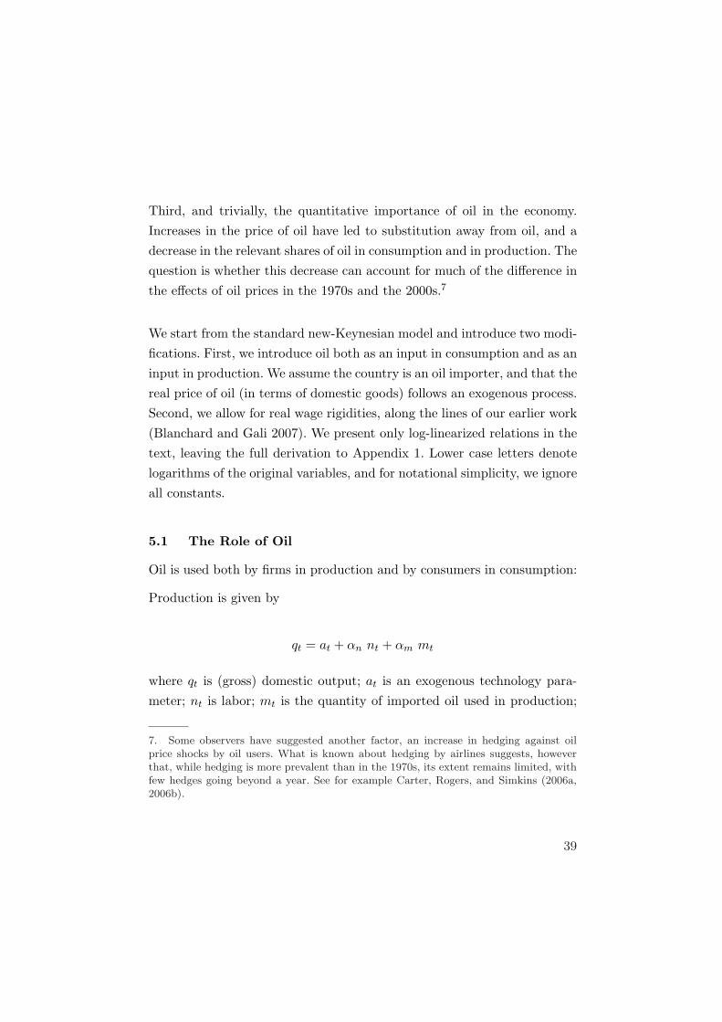
5.1 The Role of Oil
Oil is used both by firms in production and by consumers in consumption:
Production is given by
qt = at + αn nt + αm mt
where qt is (gross) domestic output; at is an exogenous technology para-meter; nt is labor; mt is the quantity of imported oil used in production;
7. Some observers have suggested another factor, an increase in hedging against oilprice shocks by oil users. What is known about hedging by airlines suggests, howeverthat, while hedging is more prevalent than in the 1970s, its extent remains limited, withfew hedges going beyond a year. See for example Carter, Rogers, and Simkins (2006a,2006b).
39

and αn + αm ≤ 1.8
Consumption is given by
ct ≡ (1− χ) cq,t + χ cm,t
where ct is consumption; cq,t is the consumption of domestically producedgoods (gross output); and cm,t is the consumption of imported oil.
In this environment, it is important to distinguish between two prices, theprice of domestic output pq,t, and the price of consumption pc,t. Let pm,t
be the price of oil, and st ≡ pm,t − pq,t be the real price of oil. From thedefinition of consumption, the relation between the consumption price andthe domestic output price is given by
pc,t = pq,t + χ st (1)
Increases in the real price of oil lead to an increase in the consumptionprice relative to the domestic output price.
5.2 Households
The behavior of households is characterized by two equations. The first isan intertemporal condition for consumption:
ct = Et{ct+1} − (it −Et{πc,t+1}) (2)
where it is the nominal interest rate, and πc,t ≡ pc,t−pc,t−1 is CPI inflation.
8. We use a Cobb–Douglas specification for convenience. It has the counterfactual im-plication that the share of oil in output remains constant. So, in our framework, whenlooking at changes in the share over time, we must attribute it to a change in the para-meter αm. For our purposes, this appears innocuous.
40
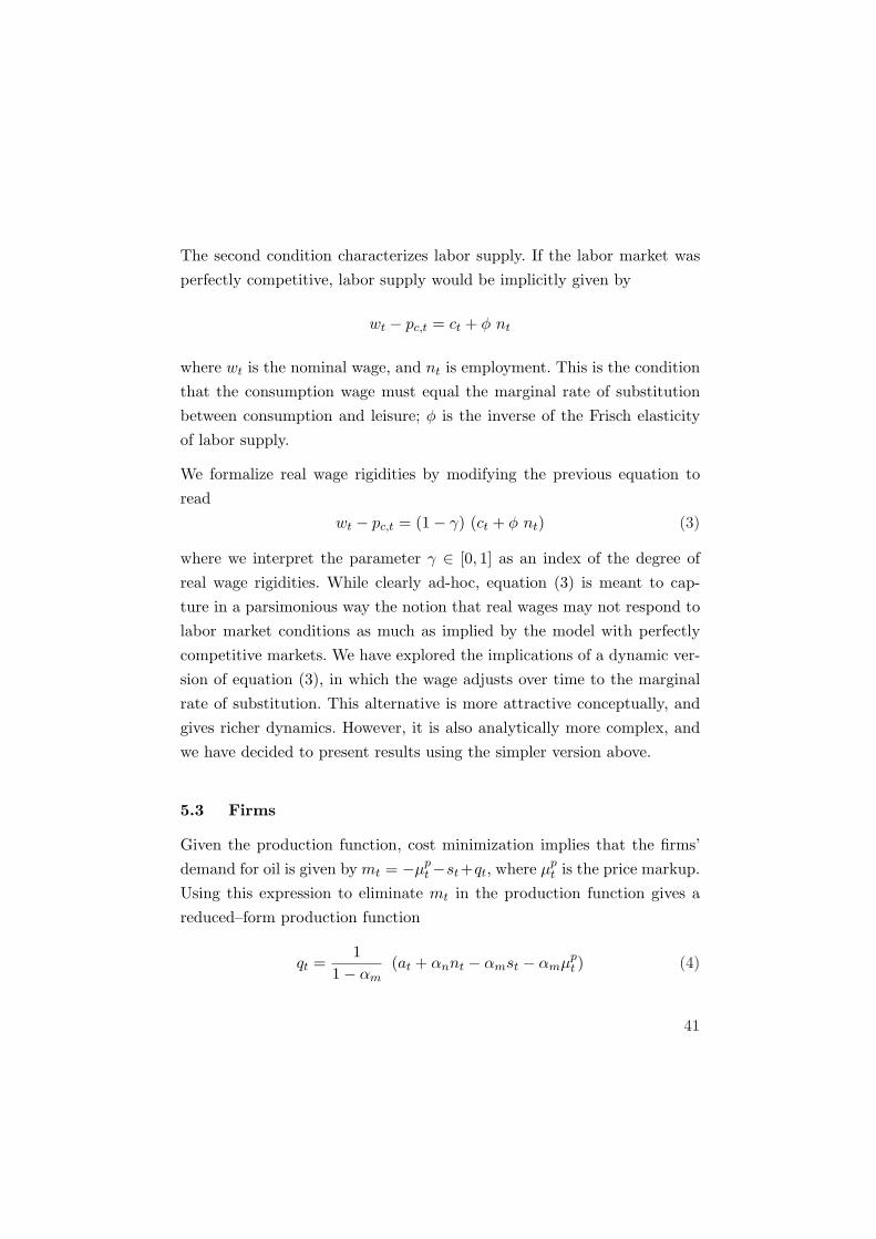
The second condition characterizes labor supply. If the labor market wasperfectly competitive, labor supply would be implicitly given by
wt − pc,t = ct + φ nt
where wt is the nominal wage, and nt is employment. This is the conditionthat the consumption wage must equal the marginal rate of substitutionbetween consumption and leisure; φ is the inverse of the Frisch elasticityof labor supply.
We formalize real wage rigidities by modifying the previous equation toread
wt − pc,t = (1− γ) (ct + φ nt) (3)
where we interpret the parameter γ ∈ [0, 1] as an index of the degree ofreal wage rigidities. While clearly ad-hoc, equation (3) is meant to cap-ture in a parsimonious way the notion that real wages may not respond tolabor market conditions as much as implied by the model with perfectlycompetitive markets. We have explored the implications of a dynamic ver-sion of equation (3), in which the wage adjusts over time to the marginalrate of substitution. This alternative is more attractive conceptually, andgives richer dynamics. However, it is also analytically more complex, andwe have decided to present results using the simpler version above.
5.3 Firms
Given the production function, cost minimization implies that the firms’demand for oil is given by mt = −µp
t −st+qt, where µpt is the price markup.
Using this expression to eliminate mt in the production function gives areduced–form production function
qt =1
1− αm(at + αnnt − αmst − αmµp
t ) (4)
41
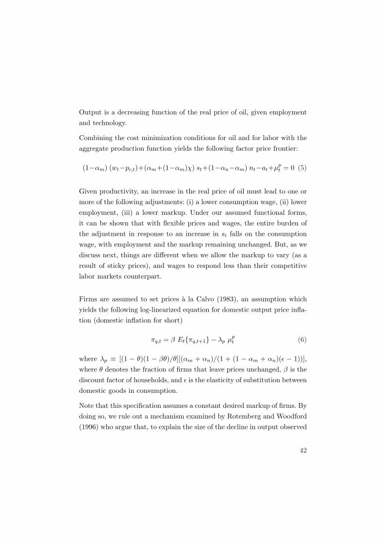
Output is a decreasing function of the real price of oil, given employmentand technology.
Combining the cost minimization conditions for oil and for labor with theaggregate production function yields the following factor price frontier:
(1−αm) (wt−pc,t)+(αm+(1−αm)χ) st+(1−αn−αm) nt−at+µpt = 0 (5)
Given productivity, an increase in the real price of oil must lead to one ormore of the following adjustments: (i) a lower consumption wage, (ii) loweremployment, (iii) a lower markup. Under our assumed functional forms,it can be shown that with flexible prices and wages, the entire burden ofthe adjustment in response to an increase in st falls on the consumptionwage, with employment and the markup remaining unchanged. But, as wediscuss next, things are different when we allow the markup to vary (as aresult of sticky prices), and wages to respond less than their competitivelabor markets counterpart.
Firms are assumed to set prices a la Calvo (1983), an assumption whichyields the following log-linearized equation for domestic output price infla-tion (domestic inflation for short)
πq,t = β Et{πq,t+1} − λp µpt (6)
where λp ≡ [(1 − θ)(1 − βθ)/θ][(αm + αn)/(1 + (1 − αm + αn)(ε − 1))],where θ denotes the fraction of firms that leave prices unchanged, β is thediscount factor of households, and ε is the elasticity of substitution betweendomestic goods in consumption.
Note that this specification assumes a constant desired markup of firms. Bydoing so, we rule out a mechanism examined by Rotemberg and Woodford(1996) who argue that, to explain the size of the decline in output observed
42
in response to oil shocks, one must assume countercyclical markups. Wedo so not because we believe the mechanism is irrelevant, but because wedo not think that variations in the degree of countercyclicality of markupsare likely to be one of the main factors behind the differences between the1970s and the 2000s.
5.4 Equilibrium
The real wage consistent with household choices (cum real wage rigidities)is given by equation (3), and depends on consumption and employment.
The real wage consistent with the firms’ factor price frontier is given byequation (5) and depends on the real price of oil, the markup, and employ-ment.
Together, these two relations imply that the markup is a function of con-sumption, employment, and the real price of oil. Solving for consumptionby using the condition that trade be balanced gives:
ct = qt − χ st + η µpt (7)
where η ≡ αm/(Mp − αm), with Mp denoting the steady state grossmarkup (now in levels). Combining this equation with the reduced formproduction function gives consumption as a function of employment, pro-ductivity, the real price of oil, and the markup
ct =1
1− αmat +
αn
1− αmnt −
(χ +
αm
1− αm
)st +
(η − αm
1− αm
)µp
t
If the steady state markup is not too large, the last term is small and cansafely be ignored. Replacing the expression for consumption in equation(3) for the consumption wage, and then replacing the consumption wagein the factor price frontier gives an expression for the markup
43
µpt = −Γn nt − Γs st + Γa at (8)
whereΓn ≡ (1− αn − αm)γ + (1− αm)(1− γ)(1 + φ)
1− (1− γ)(αm − (1− αm)η)≥ 0
Γa ≡ γ
1− (1− γ)(αm − (1− αm)η)≥ 0
Γs ≡ γ (αm + (1− αm)χ)1− (1− γ)(αm − (1− αm)η)
≥ 0
Using this expression for the markup in equation (6) gives the followingcharacterization of domestic inflation
πq,t = β Et{πq,t+1}+ λpΓn nt + λpΓs st − λpΓa at (9)
Under our assumptions, the first best level of employment can be shownto be invariant to the real price of oil: Substitution and income effectscancel.9 If γ = 0, i.e. if there are no real wage rigidities, then Γa and Γs areboth equal to zero, and domestic inflation only depends on employment.Together, these two propositions imply that stabilizing domestic inflationis equivalent to stabilizing the distance of employment from first best—aresult we have called elsewhere the “divine coincidence.”
Positive values of γ lead instead to positive values of Γa and Γs. The higherγ, or the higher (αm + (1 − αm)χ)—an expression which depends on theshares of oil in production and in consumption—the worse the trade-offbetween stabilization of employment and stabilization of domestic inflationin response to oil price shocks.
9. To see this, we can just determine equilibrium employment under perfect competitionin both goods and labor markets, corresponding to the assumptions µt = 0 for all t andγ = 0, respectively.
44
5.5 Implications for GDP and the GDP Deflator
Note that the characterization of the equilibrium did not require introduc-ing either value added or the value added deflator. But these are neededto compare the implications of the model to the data.
The value added deflator py,t is implicitly defined by pq,t = (1−αm) py,t +αm pm,t. Rearranging terms gives
py,t = pq,t − αm
1− αmst (10)
thus implying a negative effect of the real price of oil on the value addeddeflator, given domestic output prices.
The definition of value added, combined with the demand for oil, yieldsthe following relation between value added and output:
yt = qt +αm
1− αmst + η µp
t (11)
This in turn implies the following relation between value added and con-sumption:
yt = ct +(
αm
1− αm+ χ
)st (12)
An increase in the price of oil decreases consumption given value addedboth because (imported) oil is used as an input in production, and used asan input in consumption.
Under the same approximation as above, i.e.(η − αm
1−αm
)µp
t ' 0, equa-tions (4) and (11) imply the following relation between value added andemployment:
yt =1
1− αm(at + αn nt) (13)
Note that, under this approximation, the relation between value added andemployment does not depend on the real price of oil.
45
5.6 Quantifying the Effects of Oil Price Shocks
Equations (1), (2), (9), (12), and (13), describe the equilibrium dynamicsof prices and quantities, given exogenous processes for technology and thereal price of oil, and a description of how the interest rate is determined(i.e. an interest rate rule). We now use these conditions to characterize theeconomy’s response to an oil price shock.
Assume that at = 0 for all t (i.e abstract from technology shocks). It followsfrom (13) and the discussion above that the efficient level of value addedis constant (and normalized to zero) in this case. Assume further that thereal price of oil follows an AR(1) process
st = ρs st−1 + εt (14)
We can then summarize the equilibrium dynamics of value added and do-mestic inflation through the system:
πq,t = β Et{πq,t+1}+ κ yt + λpΓs st (15)
yt = Et{yt+1} − (it − Et{πq,t+1}) +αm(1− ρs)
1− αmst (16)
where κ ≡ λpΓn(1− αm)/αn.
These two equations must be complemented with a description of monetarypolicy. Assume an interest rate rule of the form
it = φπ πq,t (17)
where φπ > 1. Note that in our model πq,t corresponds to core CPI inflation,a variable that many central banks appear to focus on as the basis for theirinterest rate decisions.
46
We can then solve for the equilibrium analytically, using the method of un-determined coefficients. This yields the following expressions for domesticinflation and output:
πq,t = Ψπ st
yt = Ψy st
where
Ψπ =(1− ρs)
(κ αm1−αm
+ λpΓs
)
(1− ρs)(1− βρs) + (φπ − ρs)κ
and
Ψy =αm
1−αm(1− ρs)(1− βρs)− (φπ − ρs)λpΓs
(1− ρs)(1− βρs) + (φπ − ρs)κ
Domestic inflation and GDP follow AR(1) processes with the same first or-der coefficient as the real price of oil. Their innovations are proportional tothe innovation in the real price of oil, with the coefficient of proportionalitydepending on the parameters of the model.
Expressions for CPI inflation and employment can be obtained using (1)and (13), respectively:
πc,t = Ψπ st + χ ∆st
nt = Ψy1− αm
αnst
With these equations, we can turn to the discussion of the potential role ofthe three factors we identified earlier, real wage rigidities, monetary policy,and the quantitative importance of oil in the economy, in explaining thedifferences between the 1970s and the 2000s. In all cases we use the evidencewe presented earlier for the United States as a benchmark.
47
6 Three Hypotheses on the Changing Effects of Oil
Price Shocks
In order to assess quantitatively the potential for oil price shocks to gen-erate significant macroeconomic fluctuations, we first need to calibrate ourmodel. We assume the following parameter values:
The time unit is a quarter. We set the discount factor β equal to 0.99.We set the Calvo parameter, θ, to 0.75. We choose the elasticity of outputwith respect to labor, αn , equal to 0.7. We assume φ = 1, thus implying aunitary Frisch labor supply elasticity.
As discussed in previous sections, changes in the volatility of the real priceof oil are unlikely to lie behind the changes in the size of the effects of oilshocks. Thus, for simplicity, we assume an unchanged process for the realprice of oil. Based on an estimated AR(1) process over the period 1960:1-2006:4, we set ρs = 0.97 and var(st) = (0.11)2. Also, and unless otherwisenoted, we set the shares of oil in production and consumption (αm and χ)to equal 0.012 and 0.017, respectively, which correspond to their values in1997.
Most of the parameters above are kept constant across all the simulationspresented below. The exceptions, as well as our treatment of the remainingparameters, varies depending on the hypothesis being considered in eachcase.
6.1 Changes in Real Wage Rigidities
In the framework above, the presence of some rigidity in the adjustmentof real wages to economic conditions is a necessary ingredient in orderto generate significant fluctuations in measures of inflation and economicactivity. Figure 10 illustrates this point by showing the range of volatilitiesof CPI inflation (annualized, and expressed in percent) and GDP implied
48
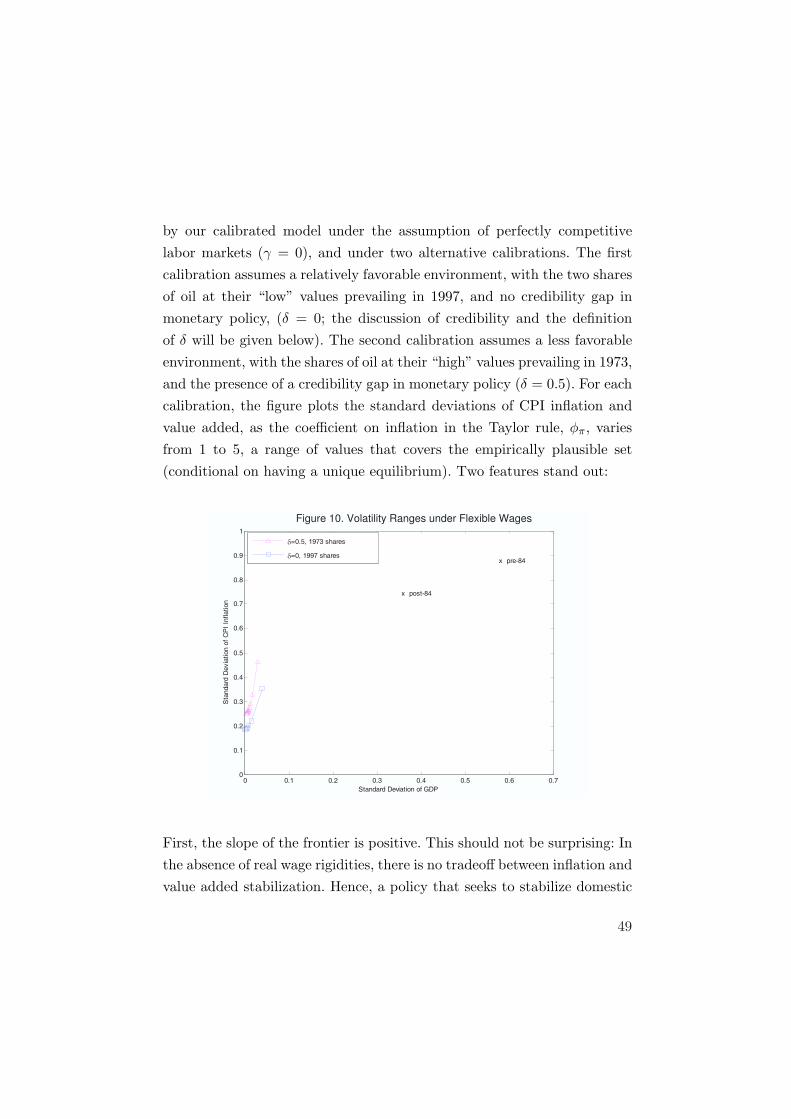
by our calibrated model under the assumption of perfectly competitivelabor markets (γ = 0), and under two alternative calibrations. The firstcalibration assumes a relatively favorable environment, with the two sharesof oil at their “low” values prevailing in 1997, and no credibility gap inmonetary policy, (δ = 0; the discussion of credibility and the definitionof δ will be given below). The second calibration assumes a less favorableenvironment, with the shares of oil at their “high” values prevailing in 1973,and the presence of a credibility gap in monetary policy (δ = 0.5). For eachcalibration, the figure plots the standard deviations of CPI inflation andvalue added, as the coefficient on inflation in the Taylor rule, φπ, variesfrom 1 to 5, a range of values that covers the empirically plausible set(conditional on having a unique equilibrium). Two features stand out:
Figure 10. Volatility Ranges under Flexible Wages
0 0.1 0.2 0.3 0.4 0.5 0.6 0.70
0.1
0.2
0.3
0.4
0.5
0.6
0.7
0.8
0.9
1
Standard Deviation of GDP
Sta
ndard
Devia
tion o
f C
PI
Inflation
=0.5, 1973 shares
=0, 1997 sharesx pre-84
x post-84
First, the slope of the frontier is positive. This should not be surprising: Inthe absence of real wage rigidities, there is no tradeoff between inflation andvalue added stabilization. Hence, a policy that seeks to stabilize domestic
49
inflation more aggressively, also stabilizes value added. In fact, one canreduce the volatility of both variables by choosing φπ to be arbitrarilylarge (this is what we called the “divine coincidence” in an earlier paper).Under the assumed rule, on the other hand, CPI inflation faces a lowerbound to its volatility, since it is affected directly by any change in theprice of oil, in proportion to the share of oil in the consumption basket.
Second, the standard deviations implied by our simulation are well belowtheir corresponding estimated conditional standard deviations, reported inTable 4 and represented by the two markers in the Figure. The volatilitygap is particularly dramatic for GDP.
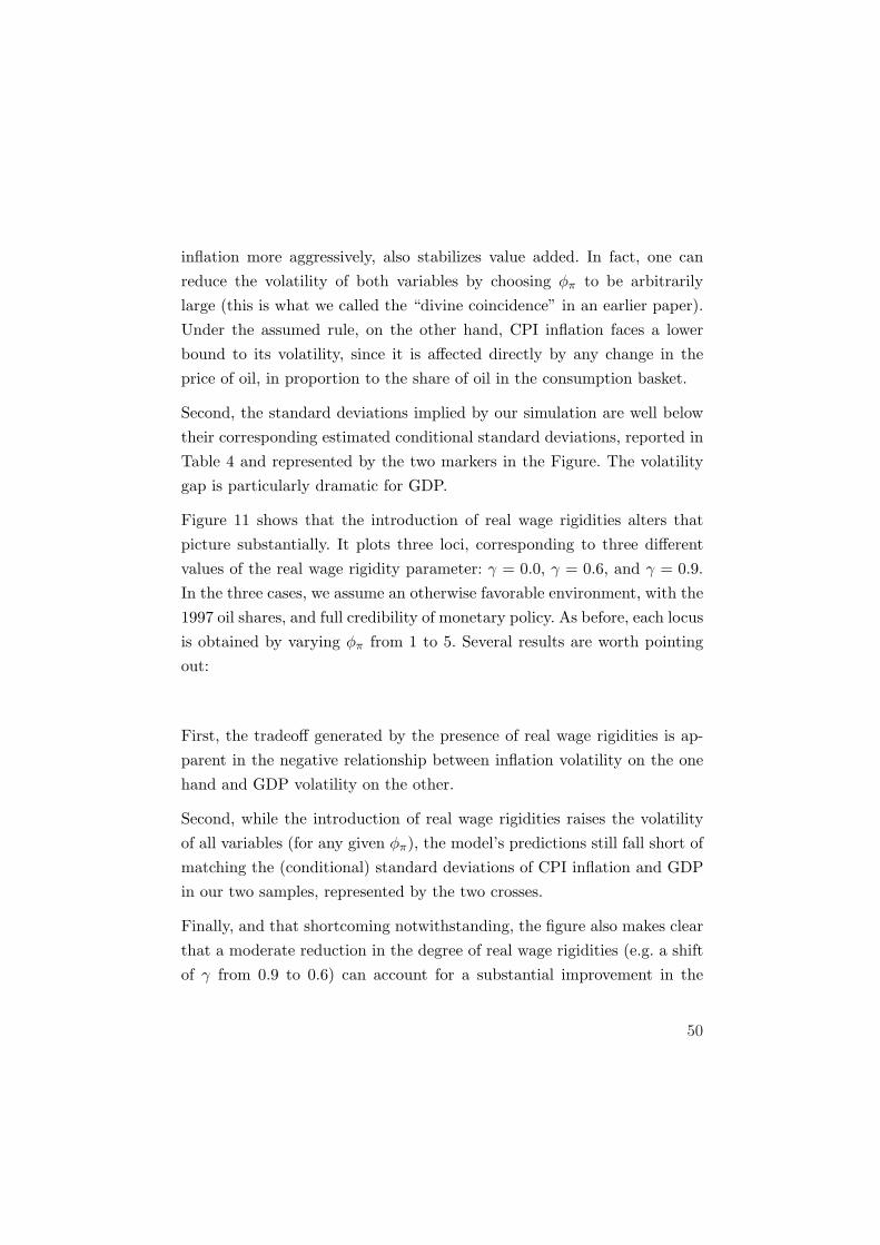
Figure 11 shows that the introduction of real wage rigidities alters thatpicture substantially. It plots three loci, corresponding to three differentvalues of the real wage rigidity parameter: γ = 0.0, γ = 0.6, and γ = 0.9.In the three cases, we assume an otherwise favorable environment, with the1997 oil shares, and full credibility of monetary policy. As before, each locusis obtained by varying φπ from 1 to 5. Several results are worth pointingout:
First, the tradeoff generated by the presence of real wage rigidities is ap-parent in the negative relationship between inflation volatility on the onehand and GDP volatility on the other.
Second, while the introduction of real wage rigidities raises the volatilityof all variables (for any given φπ), the model’s predictions still fall short ofmatching the (conditional) standard deviations of CPI inflation and GDPin our two samples, represented by the two crosses.
Finally, and that shortcoming notwithstanding, the figure also makes clearthat a moderate reduction in the degree of real wage rigidities (e.g. a shiftof γ from 0.9 to 0.6) can account for a substantial improvement in the
50
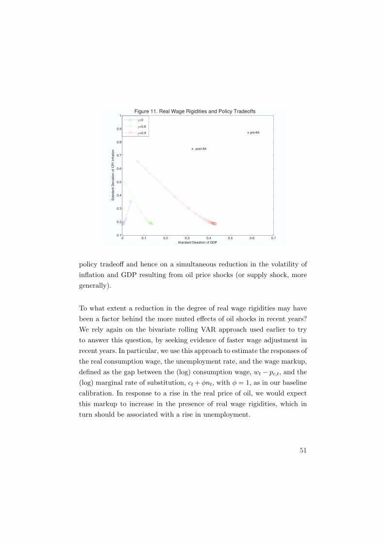
Figure 11. Real Wage Rigidities and Policy Tradeoffs
0 0.1 0.2 0.3 0.4 0.5 0.6 0.70.1
0.2
0.3
0.4
0.5
0.6
0.7
0.8
0.9
1
Standard Deviation of GDP
Sta
ndard
Devia
tion o
f C
PI
Inflation
=0
=0.6
=0.9 x pre-84
x post-84
policy tradeoff and hence on a simultaneous reduction in the volatility ofinflation and GDP resulting from oil price shocks (or supply shock, moregenerally).
To what extent a reduction in the degree of real wage rigidities may havebeen a factor behind the more muted effects of oil shocks in recent years?We rely again on the bivariate rolling VAR approach used earlier to tryto answer this question, by seeking evidence of faster wage adjustment inrecent years. In particular, we use this approach to estimate the responses ofthe real consumption wage, the unemployment rate, and the wage markup,defined as the gap between the (log) consumption wage, wt − pc,t, and the(log) marginal rate of substitution, ct + φnt, with φ = 1, as in our baselinecalibration. In response to a rise in the real price of oil, we would expectthis markup to increase in the presence of real wage rigidities, which inturn should be associated with a rise in unemployment.
51
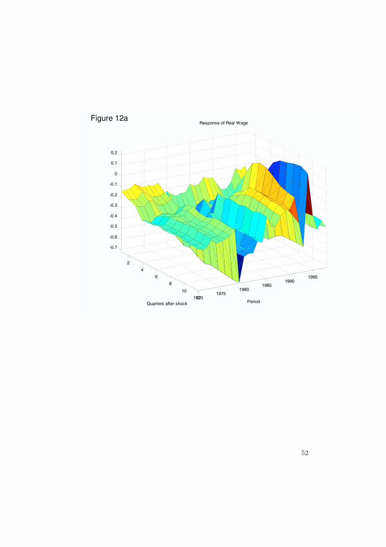
2
4
6
8
10
1219701975
19801985
19901995
-0.7
-0.6
-0.5
-0.4
-0.3
-0.2
-0.1
0
0.1
0.2
Period
Response of Real Wage
Quarters after shock
Figure 12a
52
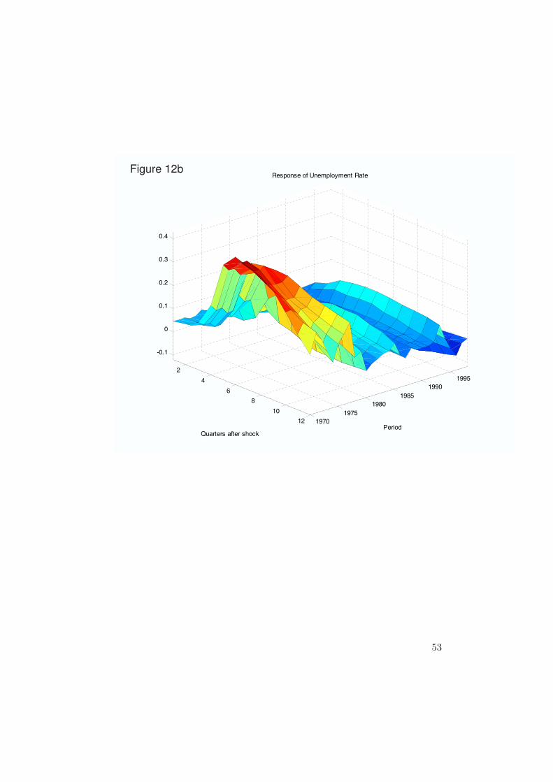
Figure 12b
2
4
6
8
10
12 1970
1975
1980
1985
1990
1995
-0.1
0
0.1
0.2
0.3
0.4
Period
Response of Unemployment Rate
Quarters after shock
53
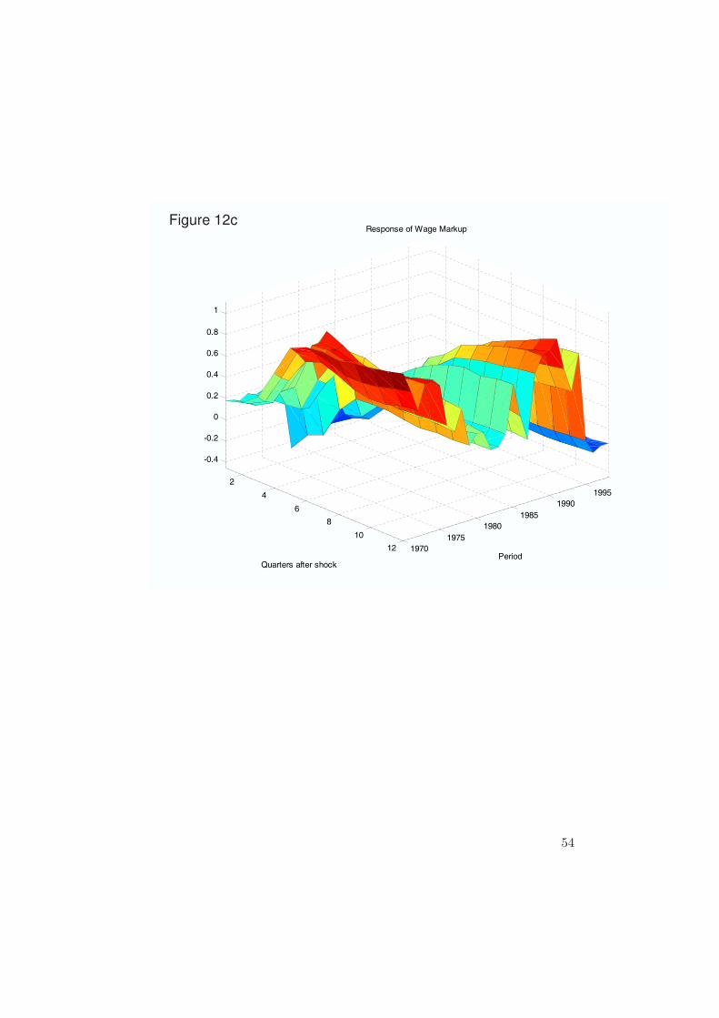
Figure 12c
2
4
6
8
10
12 1970
1975
1980
1985
1990
1995
-0.4
-0.2
0
0.2
0.4
0.6
0.8
1
Period
Response of Wage Markup
Quarters after shock
54

Figures 12a-c display the relevant IRFs representing, as before, the esti-mated response of each variable to a permanent 10 percent increase in thedollar price of oil. Figure 12a shows that the consumption wage tends todecline in response to the oil shock. While the response shows some vari-ability over time, it does not show a tendency towards a larger responseof the consumption wage over time. Figure 12b shows that unemploymenttends to increase in response to the oil shock. It also shows that this re-sponse has declined dramatically over time. An interpretation of these twoevolutions is that the decrease in real wages, which required a large increasein unemployment in the 1970s, is now achieved with barely any increase inunemployment today. This suggests, in turn, a decrease in real wage rigidi-ties. Another way of making the same point, within the logic of the model,is to look at the evolution of the wage markup. This is done in Figure 12c.An increase in the oil price leads to an increase in the wage markup: Thatis, the decrease in the consumption wage is smaller than the decrease inthe marginal rate of substitution. The effect has become, however, steadilysmaller over time, very rapidly so in the more recent period. This suggeststhat the real consumption wage moves today much more in line with themarginal rate of substitution than it did in the 1970s.10
6.2 Changes in Monetary Policy
A number of studies (e.g. Clarida, Galı, and Gertler (2000)) have providedevidence of a stronger interest rate response to variations in inflation overthe past two decades, relative to the 1960s and 1970s. It should be clear,however, from the simulations of our model presented above that, otherthings equal, a stronger anti-inflationary stance should have reduced thevolatility of inflation, but increased that of GDP. In other words, that
10. At least from a qualitative point of view, the previous evidence is robust to variationsin the calibration of parameter φ within a plausible range (which we take to be given bythe interval [0.5, 5]).
55
evidence cannot explain—at least by itself—the lower volatility of bothinflation and economic activity in response to oil price shocks.
In addition to this change in behavior, captured by the literature on em-pirical interest rate rules, there is also widespread agreement that centralbanks’ commitment to keeping inflation low and stable has also becomemore credible over the past two decades, thanks to improved communica-tions, greater transparency, the adoption of more or less explicit quantita-tive inflation targets and, ultimately, by the force of deeds. In this sectionwe use the framework developed above to study the role that such an im-provement in credibility may have had in accounting for the reduced impactof oil shocks.
We model credibility as follows: As in our baseline model we assume thatthe central bank follows an interest rate rule
it = φππq,t
The public, however, is assumed to perceive that interest rate decisions aremade according to
it = φπ(1− δ) πq,t + vt
where {vt} is taken by the public to be an exogenous i.i.d monetary policyshock, and δ ∈ [0, 1] can be interpreted as a measure of the credibilitygap. Below we restrict ourselves to calibrations that guarantee a uniqueequilibrium, which requires that the condition φπ(1− δ) > 1 be met.11
In addition to the above actual and perceived policy rules, the model isexactly as the one developed above, with the dynamics of value added,
11. The hypothesis of an indeterminate equilibrium (and, hence, the possibility ofsunspot fluctuations) in the first part of the sample could also potentially explain thegreater volatility in both inflation and GDP, as emphasized by Clarida et al. (2000).We choose to pursue an alternative line of explanation here, which does not rely onmultiplicity of equilibria.
56
domestic inflation, and the real price of oil summarized by equations (14)-(16). Solving the model for domestic inflation and value added gives:
πq,t = a st + b vt
yt = c st + d vt
where a, b, c, and d are given by:
a =(1− ρs)
(καm(1− αm)−1 + λpΓs
)
(1− ρs)(1− βρs) + (φπ(1− δ)− ρs)κ> 0
b = − κ
1 + φπ(1− δ)κ< 0
c =αm(1− αm)−1(1− ρs)(1− βρs)− (φπ(1− δ)− ρs)λpΓs
(1− ρs)(1− βρs) + (φπ(1− δ)− ρs)κ
d = − 11 + φπ(1− δ)κ
Imposing vt = δφππH,t into the solution (so that the central bank actuallyadheres to its chosen rule) we get
πq,t =a
1− bδφπst
thus implying that CPI inflation is
πc,t =a
1− bδφπst + χ ∆st
Value added is then given by:
yt = c st + dφπδ πq,t
=(
c +daφπδ
1− bδφπ
)st
57
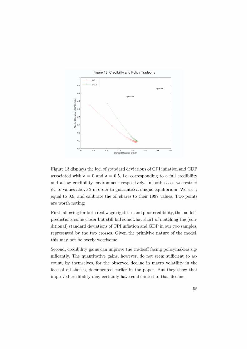
Figure 13. Credibility and Policy Tradeoffs
0 0.1 0.2 0.3 0.4 0.5 0.6 0.70.1
0.2
0.3
0.4
0.5
0.6
0.7
0.8
0.9
1
Standard Deviation of GDP
Sta
ndard
Devia
tion o
f C
PI
Inflation
=0
=0.5
x pre-84
x post-84
Figure 13 displays the loci of standard deviations of CPI inflation and GDPassociated with δ = 0 and δ = 0.5, i.e. corresponding to a full credibilityand a low credibility environment respectively. In both cases we restrictφπ to values above 2 in order to guarantee a unique equilibrium. We set γ
equal to 0.9, and calibrate the oil shares to their 1997 values. Two pointsare worth noting:
First, allowing for both real wage rigidities and poor credibility, the model’spredictions come closer but still fall somewhat short of matching the (con-ditional) standard deviations of CPI inflation and GDP in our two samples,represented by the two crosses. Given the primitive nature of the model,this may not be overly worrisome.
Second, credibility gains can improve the tradeoff facing policymakers sig-nificantly. The quantitative gains, however, do not seem sufficient to ac-count, by themselves, for the observed decline in macro volatility in theface of oil shocks, documented earlier in the paper. But they show thatimproved credibility may certainly have contributed to that decline.
58
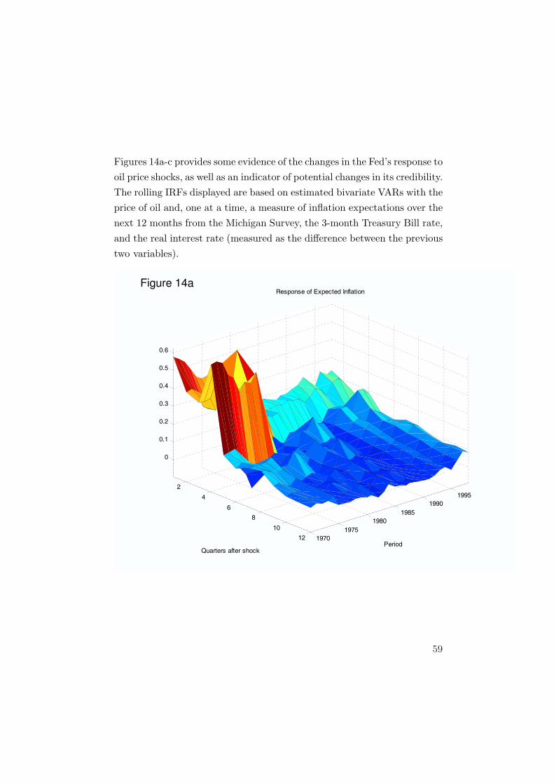
Figures 14a-c provides some evidence of the changes in the Fed’s response tooil price shocks, as well as an indicator of potential changes in its credibility.The rolling IRFs displayed are based on estimated bivariate VARs with theprice of oil and, one at a time, a measure of inflation expectations over thenext 12 months from the Michigan Survey, the 3-month Treasury Bill rate,and the real interest rate (measured as the difference between the previoustwo variables).
2
4
6
8
10
12 1970
1975
1980
1985
1990
1995
0
0.1
0.2
0.3
0.4
0.5
0.6
Period
Response of Expected Inflation
Quarters after shock
Figure 14a
59
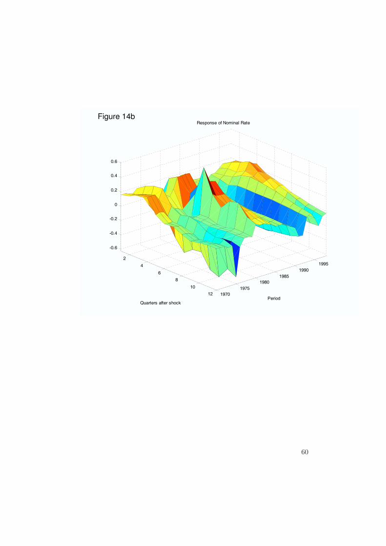
2
4
6
8
10
12 1970
1975
1980
1985
1990
1995
-0.6
-0.4
-0.2
0
0.2
0.4
0.6
Period
Response of Nominal Rate
Quarters after shock
Figure 14b
60
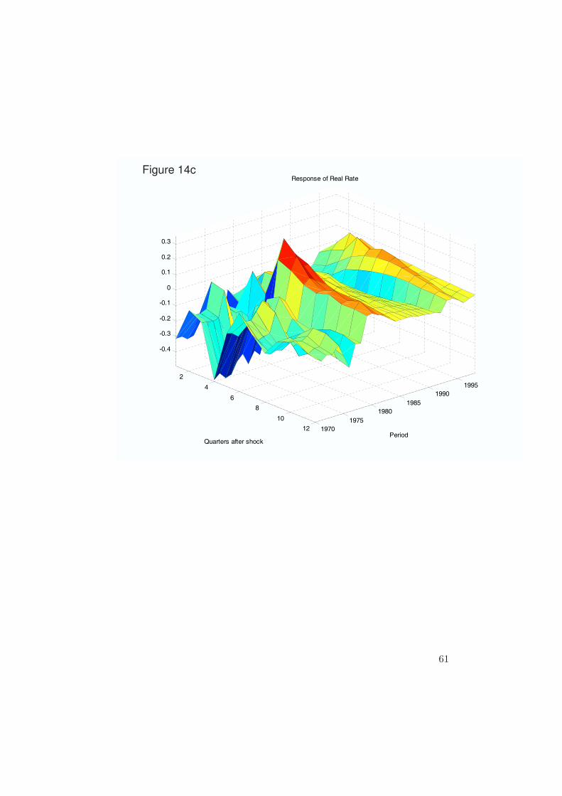
Figure 14c
2
4
6
8
10
12 1970
1975
1980
1985
1990
1995
-0.4
-0.3
-0.2
-0.1
0
0.1
0.2
0.3
Period
Response of Real Rate
Quarters after shock
61
First, and most noticeable, the response of expected inflation to an oil priceshock of the same size (normalized here to 10 percent rise) has shrunkdramatically over time, from a rise of about 50 basis points in the 1970s,to about 20 basis points since the mid-1980s, and has remained remarkablystable after that.
Second, and perhaps surprisingly, the strength of the response of the nom-inal interest rate has not changed much across sample periods. The shrink-ing response of expected inflation implies, however, that the response ofthe real rate to an oil price shock has become stronger over time. In fact,the real rate appears to decline significantly in response to an oil priceshock in the 1970s, an observation consistent with the (unconditional) ev-idence in Clarida et al. (2000). This decline may have contributed to thelarge and persistent increase in inflation. It also suggests that had the Fedpursued a stronger anti-inflationary policy (keeping credibility unchanged)the adverse effects on output and inflation would have been even larger.12
To summarize the lessons from the analysis above: While the weak responseof inflation to oil price shocks in recent years is often interpreted as aconsequence of a stronger anti-inflation stance by the Fed (a higher φπ, inthe context of out model), the evidence of a smaller decline in employmentand GDP suggests that an enhanced anti-inflation credibility may also haveplayed a role. The sharp decline in the response of inflation expectationsto an oil price shock is certainly consistent with this view.
12. Note that, for the most recent period, the real interest rate shows very little changein response to an oil price shock. There are several explanations for this finding. First,as shown above, several measures of inflation (including expected inflation and GDPdeflator inflation) hardly change in response to the oil price rise. If the Fed responds tothose measures, the required adjustment in the nominal and real rates will be relativelysmall. Secondly, the Fed may also adjust rates in response to measures of economicactivity. The decline in GDP and employment may thus have induced an interest raterate movement in the opposite direction, with the net effect being close to zero.
62
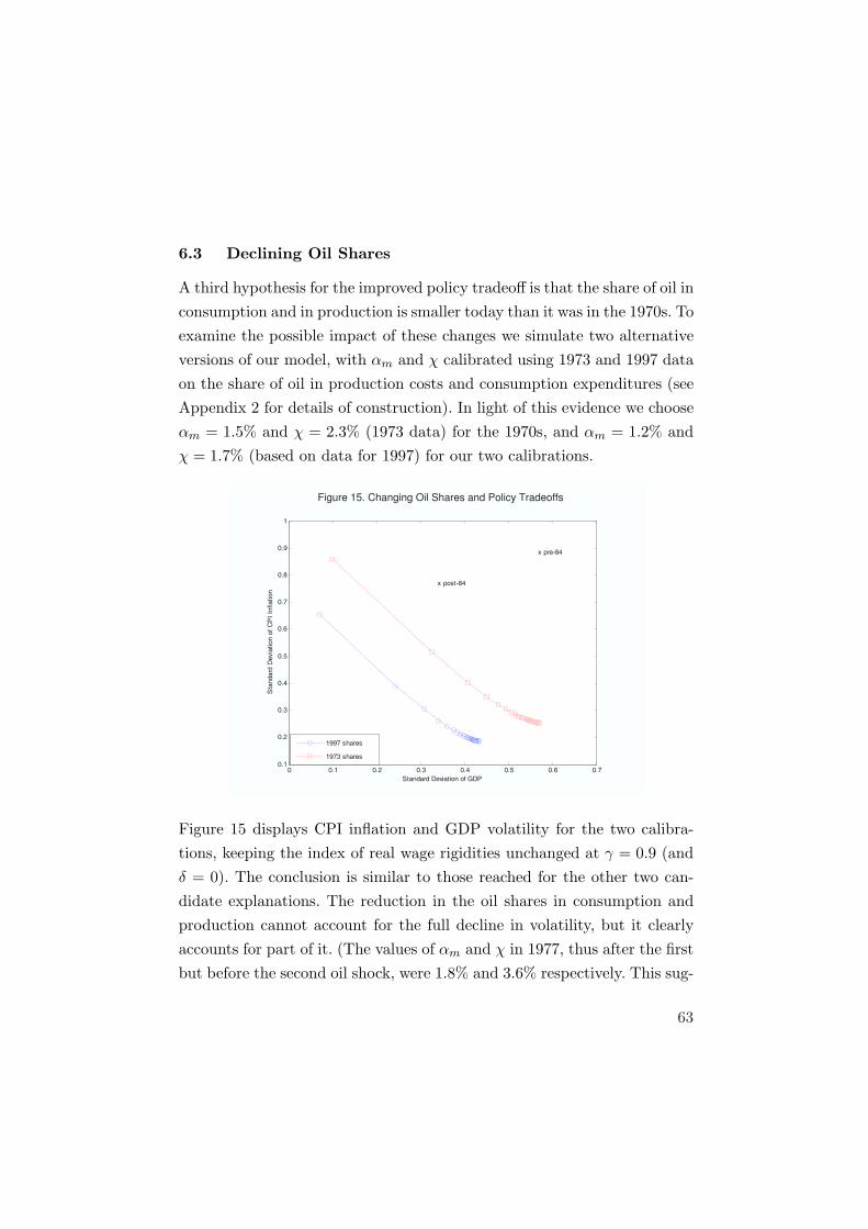
6.3 Declining Oil Shares
A third hypothesis for the improved policy tradeoff is that the share of oil inconsumption and in production is smaller today than it was in the 1970s. Toexamine the possible impact of these changes we simulate two alternativeversions of our model, with αm and χ calibrated using 1973 and 1997 dataon the share of oil in production costs and consumption expenditures (seeAppendix 2 for details of construction). In light of this evidence we chooseαm = 1.5% and χ = 2.3% (1973 data) for the 1970s, and αm = 1.2% andχ = 1.7% (based on data for 1997) for our two calibrations.
Figure 15. Changing Oil Shares and Policy Tradeoffs
0 0.1 0.2 0.3 0.4 0.5 0.6 0.70.1
0.2
0.3
0.4
0.5
0.6
0.7
0.8
0.9
1
Standard Deviation of GDP
Sta
ndard
Devia
tion o
f C
PI
Inflation
1997 shares
1973 shares
x pre-84
x post-84
Figure 15 displays CPI inflation and GDP volatility for the two calibra-tions, keeping the index of real wage rigidities unchanged at γ = 0.9 (andδ = 0). The conclusion is similar to those reached for the other two can-didate explanations. The reduction in the oil shares in consumption andproduction cannot account for the full decline in volatility, but it clearlyaccounts for part of it. (The values of αm and χ in 1977, thus after the firstbut before the second oil shock, were 1.8% and 3.6% respectively. This sug-
63

gests that, other things equal, the second oil shock should have had largereffects than the first. As we saw earlier, the opposite appears to be true.)
The analysis above has examined the effects on CPI inflation and GDPvolatility of changes in one parameter at a time. Figure 16 shows the com-bined effect of a simultaneous change in the three parameters. The firstcalibration, which is meant to roughly capture the 1970s environment,assumes strong wage rigidities (γ = 0), limited central bank credibility(δ = 0.5), and the 1973 oil shares. The second calibration assumes mildwage rigidities (γ = 0.6), full credibility (δ = 0), and the 1997 oil shares.The figure shows that our stylized model still cannot match the observed(conditional) volatility of CPI inflation and GDP; in particular it predictsa much more favorable trade-off post-1984 than is actually observed. Thefigure also shows, however, that the combination of the three changes inthe environment we have focused on can account for the improvement inthe trade-off observed in the data.
0 0.1 0.2 0.3 0.4 0.5 0.6 0.70.1
0.2
0.3
0.4
0.5
0.6
0.7
0.8
0.9
1
Standard Deviation of GDP
Sta
ndard
Devia
tion o
f C
PI
Inflation
=0.9, =0.5, 1973 shares
=0.6, =0.0, 1997 shares
x pre-84
x post-84
Figure 16. Combined Effects
64
7 Concluding Comments
We have reached five main conclusions:
First, that the effects of oil price shocks must have coincided in time withlarge shocks of a different nature. Given our partial identification strategy,we have not identified these other shocks. We have given some evidencethat increases in other commodity prices were important in the 1970s. Wehave not identified the other shocks for the 2000s.
Second, that the effects of oil price shocks have changed over time, withsteadily smaller effects on prices and wages, as well as on output and em-ployment.
Third, that a first plausible cause for these changes is a decrease in realwage rigidities. Such rigidities are needed to generate the type of largestagflation in response to adverse supply shocks such as those that tookplace in the 1970s. We have shown that the response of the consumptionwage to the marginal rate of substitution, and thus to employment, appearsto have increased over time.
Fourth, that a second plausible cause for these changes is the increasedcredibility of monetary policy. We have offered a simple formalization oflack of credibility and its effect on the volatility frontier. We have shownthat the response of expected inflation to oil shocks has substantially de-creased over time.
Fifth, that a third plausible cause for these changes is simply the decreasein the share of oil in consumption and in production. The decline is largeenough to have quantitatively significant implications.
Despite the length of the paper, we are conscious, however, of the lim-itations of our arguments. Some of the evidence, for example, the IRFevidence for Japan, does not fit our story. The model we have developed istoo primitive in many dimensions, and its quantitative implications must
65

be taken with caution. The development of a richer model, at least withrespect to the specification of production, and of real wage rigidities, andits estimation, seem the natural next steps to check the conclusions reachedabove.
66
Appendix 1: A New-Keynesian Model for an Oil-Importing
Economy
The present appendix describes in more detail the model used in Section5 and derives the equilibrium conditions underlying the simulations in themain text.
Households
We assume a continuum of identical infinitely-lived households. Each house-hold seeks to maximize
E0
∞∑
t=0
βt U(Ct, Nt)
whereCt ≡ Θχ Cχ
m,t C1−χq,t
and where Cm,t denotes consumption of (imported) oil, Cq,t ≡(∫ 1
0 Cq,t(i)1−1ε di
) εε−1
is a CES index of domestic goods, Nt denotes employment or hours worked,and Θχ ≡ χ−χ(1− χ)−(1−χ).
We assume that period utility is given by
U(Ct, Nt) ≡ log Ct − N1+φt
1 + φ
The period budget constraint, conditional on optimal allocation of expen-ditures among different domestic goods (not derived here) is given by:
Pq,tCq,t + Pm,tCm,t + QBt Bt = WtNt + Bt−1 + Πt
where Pq,t ≡(∫ 1
0 Pq,t(i)1−ε di) 1
1−ε is a price index for domestic goods, Pm,t
is the price of oil (in domestic currency), and Wt is the nominal wage. QBt
is the price of a one-period nominally riskless domestic bond, paying one
67
unit of domestic currency. Bt denotes the quantity of that bond purchasedin period t. For simplicity we assume no access to international financialmarkets.
The optimal allocation of expenditures between imported and domesticallyproduced good implies
Pq,tCq,t = (1− χ) Pc,tCt
Pm,tCm,t = χ Pc,tCt
where Pc,t ≡ Pχm,t P 1−χ
q,t is the CPI index. Note that χ corresponds, in equi-librium, to the share of oil in consumption. Note also that Pc,t ≡ Pq,t Sχ
t ,where St ≡ Pm,t
Pq,tdenotes the real price of oil,expressed in terms of domes-
tically produced goods. Taking logs,
pc,t = pq,t + χ st
where st ≡ pm,t − pq,t is the log of the real price of oil (measured in termsof domestic goods).
Furthermore, and conditional on an optimal allocation between the twotypes of goods, we have Pq,tCq,t + Pm,tCm,t = Pc,tCt, which can be substi-tuted into the budget constraint. The resulting constraint can then be usedto derive the household’s remaining optimality conditions. The intertem-poral optimality condition is given by:
QBt = β Et
{Ct
Ct+1
Pc,t
Pc,t+1
}
Under the assumption of perfect competition in labor markets (to be re-laxed below), the household’s intratemporal optimality condition is given
68
byWt
Pc,t= Ct Nφ
t ≡ MRSt
which is the perfectly competitive labor supply schedule. The log-linearizedversion of the previous two equations, found in the text, are given by:
ct = Et{ct+1} − (it − Et{πc,t+1} − ρ) (18)
wt − pc,t = ct + φ nt (19)
where we use lower-case letters to denote the logarithms of the originalvariables, and where πc,t ≡ pc,t − pc,t−1 represents CPI inflation.
Firms
Each firm produces a differentiated good indexed by i ∈ [0, 1] with a pro-duction function
Qt(i) = At Mt(i)αmNt(i)αn
where αm + αn ≤ 1.
Independently of how prices are set, and assuming that firms take the priceof both inputs as given, cost minimization implies that firm i’s nominalmarginal cost Ψt(i) is given by:
Ψt(i) =Wt
αn(Qt(i)/Nt(i))=
Pm,t
αm(Qt(i)/Mt(i))(20)
Letting Mpt (i) ≡ Pq,t(i)/Ψt(i) denote firm i’s gross markup, we have
Mpt (i) StMt(i) = αm Qt(i)
Pq,t(i)Pq,t
Let Qt ≡(∫ 1
0 Qt(i)1−1ε di
) εε−1 denote aggregate gross output. It follows
69
thatMt =
αm Qt
Mpt St
(21)
where we have used the fact that Qt(i) = (Pq,t(i)/Pq,t)−ε Qt (the demandschedule facing firm i), and defined Mp
t as the average gross markup,weighted by firms’ input shares.
Taking logs and ignoring constants
mt = −µpt − st + qt
where µpt ≡ logMp
t . The latter expression can be plugged back into the(log linearized) aggregate production function to yield the reduced formgross output equation
qt =1
1− αm(at + αnnt − αmst − αmµp
t ) (22)
Consumption and Gross Output
Note that in an equilibrium with balanced trade (and hence Bt = 0) thefollowing relation must hold:
Pc,tCt = Pq,tQt − Pm,tMt
=(
1− αm
Mpt
)Pq,tQt
where we have used (21) to derive the second equality. Taking logs andusing the relations between the different price indexes, we obtain
ct = qt − χ st + η µpt (23)
where η ≡ αmMp−αm
and Mp denotes the steady state markup.
70
Combining (22) and (23), and invoking the fact that(
αmMp−αm
− αm1−αm
)µp
t '0 for plausibly low values of αm and the net markup measures Mp− 1 andµp
t , we can write
ct =1
1− αmat +
αn
1− αmnt −
(αm
1− αm+ χ
)st (24)
Gross Output, Value Added, and the GDP Deflator
The GDP deflator Py,t is implicitly defined by
Pq,t ≡ (Py,t)1−αm (Pm,t)αm
Taking logs and using the definition of the terms of trade st
py,t = pq,t − αm
1− αmst
Value added (or GDP), Yt, is then defined by
Py,tYt ≡ Pq,tQt − Pm,tMt
=(
1− αm
Mpt
)Pq,tQt
which can be log linearized to yield
yt = qt +αm
1− αmst + η µp
t
=1
1− αm(at + αn nt)
where the last equality uses the approximation invoked above.
Note that combining the above expressions for consumption and value
71
added we can obtain the following relation between the two
ct = yt −(
αm
1− αm+ χ
)st
Price Setting
Here we assume that firms set prices in a staggered fashion, as in Calvo(1983). Each period only a fraction 1− θ of firms, selected randomly, resetprices. The remaining firms, with measure θ, keep their prices unchanged.The optimal price setting rule for a firm resetting prices in period t is givenby
Et
{ ∞∑
k=0
θk Λt,t+k Qt+k|t(P ∗
t −Mp Ψt+k|t)}
= 0 (25)
where P ∗t denotes the price newly set at time t, Qt+k|t and Ψt+k|t are
respectively the level of output and marginal cost in period t+k for a firmthat last set its price in period t, and Mp ≡ ε/(ε− 1) is the desired grossmarkup. Note that the latter also corresponds to the gross markup in thezero inflation perfect foresight steady state.
The domestic price level evolves according to the difference equation
Pq,t =[θ (Pq,t−1)1−ε + (1− θ) (P ∗
t )1−ε] 1
1−ε (26)
Combining the log-linearized version of (25) and (26) around a zero in-flation steady state, yields the following equation for domestic inflation,πq,t ≡ pq,t − pq,t−1:
πq,t = β Et{πq,t+1} − λp µpt (27)
where µpt ≡ µp
t −µp denotes the (log) deviation of the average markup fromits desired level, and λp ≡ (1−θ)(1−βθ)
θ1−αk
1−αk+αkε .
72
Appendix 2. Computation of the Oil Share
We think of the U.S. economy as having two sectors, an oil-producingsector and a non-oil producing sector. We define the oil producing sectoras the sum of the “oil and gas extraction” sector (NAIC code 211) and the“petroleum and coal” sector (NAIC code 324). (“Petroleum refineries”, asubsector of “petroleum and coal” is available only for benchmark years,the last available one being 1997. It represents 85% of the gross output ofthe “petroleum and coal” sector.) We define the non-oil producing sectoras the rest of the economy.
To compute relevant numbers for 2005, we use data from the IO tablesfrom the BEA site.
In 2005, “oil and gas extraction” output was $227b, imports were $223b,for a total of $450b. Of this total, $5b was for domestic final uses, $440bwas for intermediates, of which $259 went to “Petroleum and coal”, and$181b went to the non-oil sector. Petroleum and coal output was $402b,imports were $65b, for a total of $467b. Of this total, $167 was for domesticfinal uses, $279b for intermediates to the non-oil producing sector.
In 2005, total U.S. value added was $12,455b. Value added by “oil and gas”was $12b, value added by “petroleum and coal” was $12b, so value addedin the non oil-producing sector was $12,431b.
These numbers imply a value for χ of (181+279)/(12,431+181+279)=3.5%, and an estimate of α is (5+167)/(12,431+181+279)= 1.3%.
The shares obviously depend very much on the price of oil. The same com-putation for the benchmark year of 1997 (which allows us to use “petroleumrefining” rather than “petroleum and coal” together) gives 1.7% and 1.2%respectively.
For the years 1973 and 1977, sectors are classified according to indus-try number codes. We construct the oil-producing sector as the sum of
73
of “crude petroleum and natural gas” (1977 industry number 8) and “pe-troleum refining” (1977 industry number 31). The same steps as aboveyield χ = 2.3% and α = 1.5% in 1973, and χ = 3.6% and α = 1.8% in1977.
74
REFERENCES
Barsky, Robert, and Lutz Killian (2002): “Do We Really Know that OilCaused the Great Stagflation? A Monetary Alternative,” NBER Macro-economics Annual 2001, May, 137-183.
Bernanke, Ben, Mark Gertler, and Mark Watson, (1997): “Systematic Mon-etary Policy and the Effects of Oil Shocks,” Brookings Papers on EconomicActivity, 1997-1, 91-157.
Blanchard, Olivier, and John Simon (2001): “The Long and Large Declinein U.S. Output Volatility,” Brookings Papers on Economic Activity, 2001-1,135-174.
Blanchard, Olivier, and Jordi Gali (2007): “Real wage rigidities and theNew-Keynesian model,” Journal of Money, Credit, and Banking, forth-coming.
Bruno, Michael, and Jeffrey Sachs, (1985): Economics of Worldwide Stagfla-tion, Harvard University Press: Cambridge Massachusetts.
Calvo, Guillermo (1983): “Staggered Contracts in a Utility-MaximizingFramework,” Journal of Monetary Economics, September, 12, 383-398.
Carter, David, Daniel Rogers, and Betty Simkins, (2006): “Does Fuel Hedg-ing Make Economic Sense? The Case of the U.S. Airline Industry,”FinancialManagement, 35–1, Spring.
Carter, David, Daniel Rogers, and Betty Simkins, (2006): “Hedging andValue in the U.S. Airline Industry,”Journal of Applied Corporate Finance,18-4, 21–33, Fall.
Castelnuovo, Efrem, Sergio Nicoletti-Altimari, and Diego Rodriguez-Palenzuela(2003): “Definition of Price Stability, Range and Point Inflation Targets:The Anchoring of Long Term Inflation Expectations,” in Background Stud-ies for the ECB’s Evaluation of its Monetary Policy Strategy.
75
Clarida, Richard, Jordi Gali, and Mark Gertler (2000): “Monetary PolicyRules and Macroeconomic Stability: Evidence and Some Theory,” Quar-terly Journal of Economics, 115-1, February, 147-180.
De Gregorio, Jose, Oscar Landerretche, and Christopher Neilson (2007):“Another Passthrough Bites the Dust? Oil Prices and Inflation,” mimeo.
Edelstein, Paul, and Lutz Kilian (2007): “Retail Energy Prices and Con-sumer Expenditures,” University of Michigan, mimeo.
Erceg, Christopher, Dale Henderson and Andrew Levin (2000): “OptimalMonetary Policy with Staggered Wage and Price Contracts,” Journal ofMonetary Economics, 46, 281-313.
Finn, Mary G. (2000): “Perfect Competition and the Effects of EnergyPrice Increases on Economic Activity,” Journal of Money Credit and Bank-ing, vol. 32, no. 3., 400-416.
Hamilton, James (1983): “Oil and the Macroeconomy since World War II,”Journal of Political Economy, April 1983, 228-248
Hamilton, James (1996): “This is What Happened to the Oil Price Macro-economy Relationship,” Journal of Monetary Economics, vol 38, no2, Oc-tober, 215-220.
Herrera,Ana Marıa and Elena Pesavento (2007): “Oil Price Shocks, System-atic Monetary Policy, and the Great Moderation,” Michigan State Univer-sity, unpublished manuscript.
Hooker, Mark A. (1996): “What Happened to the Oil Price MacroeconomyRelationship?,” Journal of Monetary Economics, 38, 195-213.
Hooker, Mark A. (2002): “Are Oil Shocks Inflationary? Asymmetric andNonlinear Specifications versus Changes in Regime,” Journal of Money,Credit and Banking, vol. 34, no. 2, 540-561.
Kilian, Lutz (2006): “Not All Oil Price Shocks Are Alike: Disentangling
76

Demand and Supply Shocks in the Crude Oil Market,” CEPR DiscussionPaper 5994.
Kilian, Lutz (2007): “A Comparison of the Effects of Exogenous Oil Sup-ply Shocks on Output and Inflation in the G7 Countries,” Journal of theEuropean Economic Association, forthcoming.
Levin, Andrew T., Fabio M. Natalucci, and Jeremy M. Piger (2004): “TheMacroeconomic Effects of Inflation Targeting,” Federal Reserve Bank ofSt. Louis Review, vol. 86, no. 4, 51-80.
Mankiw, N. Gregory (2006): Macroeconomics, 6th edition, Worth Publish-ers.
McConnell, Margaret, and Gabriel Perez-Quiros (2000): “Output Fluctu-ations in the United States; What Has Changed Since the Early 1980s?,”American Economic Review, 90-5, December, 1464-1476.
Rotemberg, Julio and Michael Woodford (1996): “Imperfect Competitionand the Effects of Energy Price Increases on Economic Activity,” Journalof Money, Credit and Banking, vol. 28, no. 4, 549-577.
Stock, James, and Mark Watson (2003): “Has the Business Cycle Changedand Why?,” Federal Reserve Bank of Kansas City, 9-56.
77