issn 1936-5330

Monetary Conservatism and Fiscal Policy1

Klaus Adam2

Roberto Billi3

First version: February 2007

This version: July 2008

RWP 07-01

Abstract: Does an inflation conservative central bank à la Rogoff (1985) remain desirable in a setting with endogenous fiscal policy? To provide an answer we study monetary and fiscal policy games without commitment in a dynamic, stochastic sticky-price economy with monopolistic distortions. Monetary policy determines nominal interest rates and fiscal policy provides public goods generating private utility. We find that lack of fiscal commitment gives rise to excessive public spending. The optimal inflation rate internalizing this distortion is positive, but lack of monetary commitment generates too much inflation. A conservative monetary authority thus remains desirable. When fiscal policy is determined before monetary policy each period, the monetary authority should focus exclusively on stabilizing inflation. Monetary conservatism then eliminates the steady state biases associated with lack of monetary and fiscal commitment and leads to stabilization policy that is close to optimal. Keywords: sequential non-cooperative policy games, discretionary policy, time consistent policy, conservative monetary policy JEL Classification: E52, E62, E63

1 We thank Marina Azzimonti, Helge Berger, V.V. Chari, Gauti Eggertsson, Jordi Galí, Albert Marcet, Ramon Marimon, Chris Waller, seminar participants at IGIER/Bocconi University, participants at the Third Conference of the International Research Forum on Monetary Policy and the 11th International Conference on Computing in Economics and Finance for helpful comments and discussions. Errors remain ours.. The views expressed herein are solely those of the author and do not necessarily reflect the views of the Federal Reserve Bank of Kansas City or the Federal Reserve System. 2 Mannheim University, Department of Economics, L7, 3-5, 68131 Mannheim, Germany; and CEPR, London; email: adam@mail.uni-mannheim.de 3 Federal Reserve Bank of Kansas City, One Memorial Drive, Kansas City, MO 64198, United States, E-mail: Roberto.Billi@kc.frb.org

1 Introduction

Which monetary institutions can overcome the problems associated with lack of monetary

commitment? A prominent early answer is Rogo¤�s (1985) proposal to appoint an in�ation

conservative central banker. This and other well-known proposals1 assume, however, that �scal

policy can be treated as exogenous when studying the design of monetary institutions. While

this assumption is a useful starting point, it is an unsatisfactory aspect of previous studies.

In this paper we ask whether installing a conservative central banker remains desirable when

�scal policy is endogenous and equally subject to a commitment problem.

We analyze a non-cooperative monetary and �scal policy game within a standard sto-

chastic general equilibrium model without capital, along the lines of Rotemberg (1982) and

Woodford (2003). This economy features three sources of distortions: (1) �rms operate under

monopolistic competition, which causes output to be ine¢ ciently low; (2) prices are rigid in

the short-term, which gives rise to real e¤ects of monetary policy; (3) policymakers cannot

credibly commit to a path for future policy, but instead determine policy sequentially.

In line with recent monetary policy models, the monetary authority determines the short-

term nominal interest rate. We add to this setting a �scal authority which decides the level

of public goods provision. Public goods generate utility for private agents and are �nanced

by lump sum taxes, so as to balance the government�s intertemporal budget.2

While the monetary and �scal authority are benevolent, i.e., maximize the utility of the

representative agent, lack of commitment gives rise to suboptimal policy outcomes. Since out-

put is ine¢ ciently low, both policymakers are tempted to increase output, either via lowering

real interest rates (monetary authority) or via increasing public spending (�scal authority).

1See for example Svensson (1997) and Walsh (1995).2Our results extend to a setting with distortionary labor taxes, as shown in a companion note. See Adam

and Billi (2008).

1

This results in an in�ationary bias and in overspending on public goods, compared to a sit-

uation with policy commitment, because with sequential decision making both policymakers

fail to fully internalize the welfare cost of generating in�ation today.

In our setting monetary and �scal policy interact in interesting ways. Speci�cally, taking

the lack of �scal commitment as given makes it optimal for monetary policy to aim at positive

in�ation rates. We show that positive in�ation rates reduce the �scal spending bias and

thereby increase welfare. This suggests that, unlike in the standard case with exogenous

�scal policy, a conservative central bank may not always be desirable. A quantitative exercise

suggests, however, that the optimal deviations from price stability tend to be small. Moreover,

in the non-cooperative Markov-perfect Nash equilibrium with sequential monetary and �scal

policy, the in�ation rate lies signi�cantly above the optimal in�ation rate for a wide range of

model parameterizations.3 This result suggests that installing an in�ation conservative central

banker is desirable also with endogenous �scal policy.

We then formally introduce a conservative monetary authority that maximizes a weighted

sum of an in�ation loss term and the representative agent�s utility. And we characterize the

resulting Markov-perfect equilibria.

When policies are determined simultaneously or when monetary policy is determined before

�scal policy each period, monetary conservatism alone cannot eliminate entirely the steady

state distortions from sequential policymaking. There is positive in�ation or �scal overspend-

ing, or both. Nevertheless, we �nd that a su¢ ciently high degree of monetary conservatism

eliminates most of the steady state welfare loss arising from the lack of monetary and �scal

commitment.

Monetary conservatism turns out to be even more desirable if �scal policy is determined

before monetary policy each period (arguably the most relevant timing protocol). In such

3Markov-perfect Nash equilibria, as de�ned in Maskin and Tirole (2001), are a standard re�nement used

in the applied dynamic games literature, e.g., Klein et al. (2008).

2

a setting monetary conservatism is internalized by �scal policy, which makes it possible to

eliminate entirely the steady state biases stemming from lack of monetary and �scal commit-

ment, provided the monetary authority cares exclusively about in�ation. Overall, the case for

a conservative monetary authority thus remains stronger in a setting with endogenous �scal

policy.

We also address the issue of how the conduct of stabilization policy is a¤ected by monetary

conservatism. We show that �scal leadership in combination with a fully conservative central

banker can achieve the �exible-price Ramsey allocation following technology and mark-up

shocks. This result suggests that monetary conservatism is desirable also from the viewpoint

of cyclical stabilization policy.

Following the work of Kydland and Prescott (1977) and Barro and Gordon (1983), the

monetary policy literature has extensively studied time-inconsistency problems in dynamic

settings and its potential solutions, see Rogo¤ (1985), Svensson (1997) and Walsh (1995). In

this literature, �scal policy is typically absent or exogenous to the model. At the same time,

a number of contributions analyze the time-consistency of optimal �scal plans in dynamic

general equilibrium models, e.g., Lucas and Stokey (1983), Chari and Kehoe (1990) or Klein,

Krusell, and Ríos-Rull (2008). But this literature typically studies models without money.

The next section introduces the model and the implementability constraints characteriz-

ing private-sector behavior. Section 3 derives monetary and �scal policy with and without

commitment and some analytical results about the policy biases. In section 4 we quantify the

biases and their welfare implications. Section 5 studies monetary conservatism and section

6 explains the robustness of the results to distortionary taxation. The technical material is

available in the web appendix to this paper.

3

2 The Model

The setting is a sticky-price economy with monopolistic competition, similar to the one studied

in Schmitt-Grohé and Uribe (2004).

2.1 Private Sector

There is a continuum of identical households with preferences given by

E0

1Xt=0

�tu(ct; ht; gt) (1)

where ct is consumption of an aggregate consumption good, ht 2 [0; 1] labor e¤ort, gt public

goods provision by the government in the form of aggregate consumption goods, and � 2 (0; 1)

the discount factor. Utility is separable in c; h; g and uc > 0, ucc < 0, uh < 0, uhh � 0, ug > 0,

ugg < 0, and��� cuccuc ���,���huhhuh

��� are bounded.Each household produces a di¤erentiated intermediate good. Demand for this good is

ytd( ePt=Pt), where yt is (private and public) demand for the aggregate good and ePt=Pt therelative price of the intermediate good compared to the aggregate good. The demand function

d(�) satis�es d(1) = 1 and d0(1) = �t, where �t 2 (�1;�1) is the price elasticity of demand for

the di¤erent goods. This elasticity is time-varying and induces �uctuations in the monopolistic

mark-up charged by �rms. The demand function is consistent with optimizing individual

behavior when private and public consumption goods are a Dixit-Stiglitz aggregate of the

goods produced by di¤erent households. The household chooses ePt, then hires the necessaryamount of labor e¤ort eht to satisfy the resulting product demand, i.e.,

zt eht = ytd ePtPt

!(2)

where zt is an aggregate technology shock. The mark-up shock �t and the technology shock

zt follow independent AR(1) stochastic processes with autocorrelation coe¢ cients �� and �z

and steady state values z = 1 and � < �1.

4

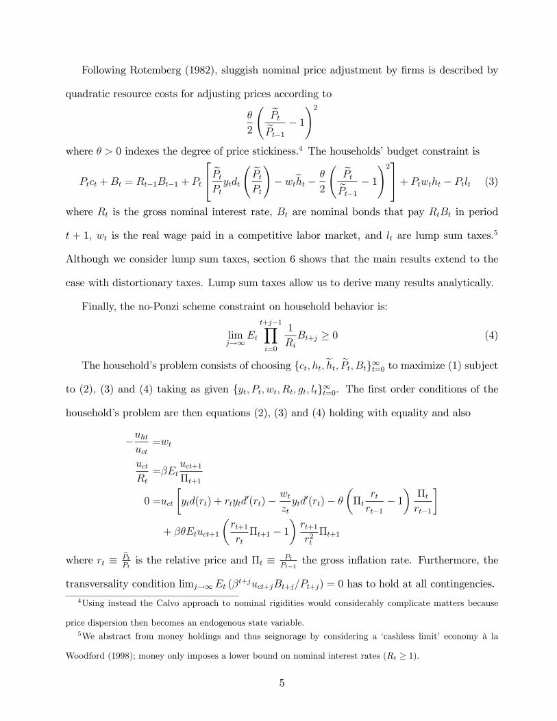
Following Rotemberg (1982), sluggish nominal price adjustment by �rms is described by

quadratic resource costs for adjusting prices according to

�

2

ePtePt�1 � 1!2

where � > 0 indexes the degree of price stickiness.4 The households�budget constraint is

Ptct +Bt = Rt�1Bt�1 + Pt

24 ePtPtytdt

ePtPt

!� wteht � �

2

ePtePt�1 � 1!235+ Ptwtht � Ptlt (3)

where Rt is the gross nominal interest rate, Bt are nominal bonds that pay RtBt in period

t + 1, wt is the real wage paid in a competitive labor market, and lt are lump sum taxes.5

Although we consider lump sum taxes, section 6 shows that the main results extend to the

case with distortionary taxes. Lump sum taxes allow us to derive many results analytically.

Finally, the no-Ponzi scheme constraint on household behavior is:

limj!1

Et

t+j�1Yi=0

1

RiBt+j � 0 (4)

The household�s problem consists of choosing {ct; ht;eht; ePt; Bt}1t=0 to maximize (1) subjectto (2), (3) and (4) taking as given {yt; Pt; wt; Rt; gt; lt}1t=0. The �rst order conditions of the

household�s problem are then equations (2), (3) and (4) holding with equality and also

�uhtuct

=wt

uctRt=�Et

uct+1�t+1

0 =uct

�ytd(rt) + rtytd

0(rt)�wtztytd

0(rt)� ���t

rtrt�1

� 1��trt�1

�+ ��Etuct+1

�rt+1rt�t+1 � 1

�rt+1r2t�t+1

where rt �ePtPtis the relative price and �t � Pt

Pt�1the gross in�ation rate. Furthermore, the

transversality condition limj!1Et (�t+juct+jBt+j=Pt+j) = 0 has to hold at all contingencies.

4Using instead the Calvo approach to nominal rigidities would considerably complicate matters because

price dispersion then becomes an endogenous state variable.5We abstract from money holdings and thus seignorage by considering a �cashless limit� economy à la

Woodford (1998); money only imposes a lower bound on nominal interest rates (Rt � 1).

5

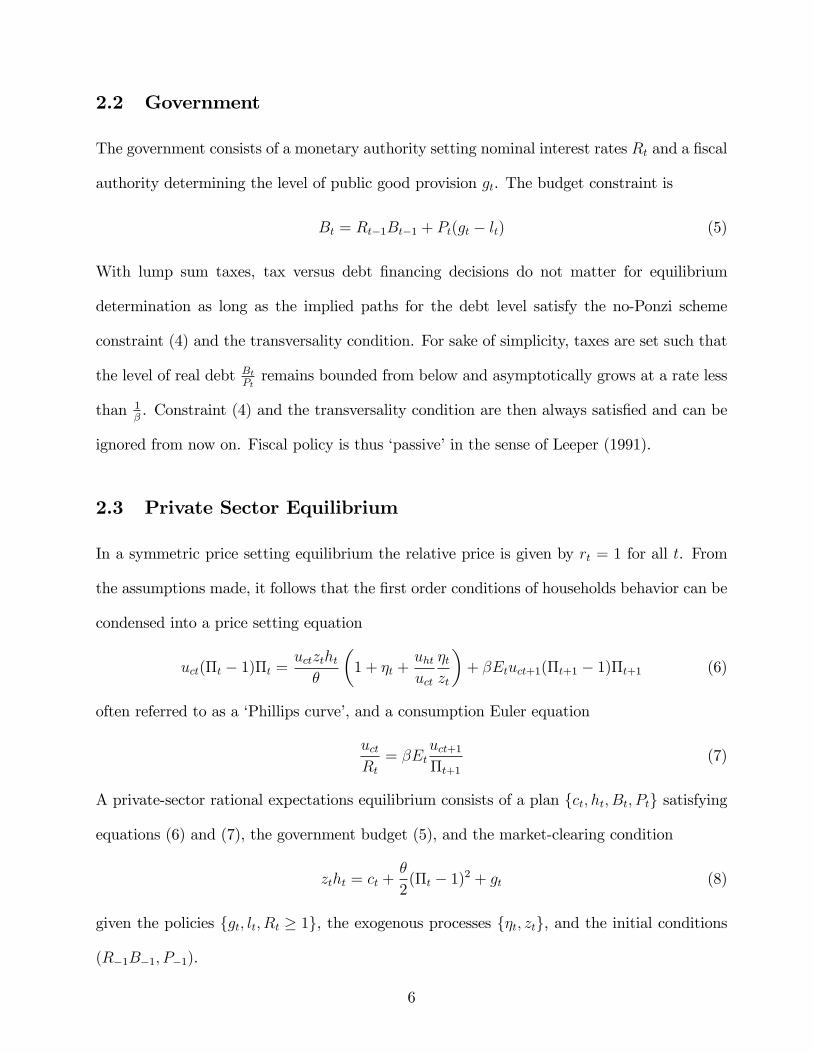
2.2 Government

The government consists of a monetary authority setting nominal interest rates Rt and a �scal

authority determining the level of public good provision gt. The budget constraint is

Bt = Rt�1Bt�1 + Pt(gt � lt) (5)

With lump sum taxes, tax versus debt �nancing decisions do not matter for equilibrium

determination as long as the implied paths for the debt level satisfy the no-Ponzi scheme

constraint (4) and the transversality condition. For sake of simplicity, taxes are set such that

the level of real debt BtPtremains bounded from below and asymptotically grows at a rate less

than 1�. Constraint (4) and the transversality condition are then always satis�ed and can be

ignored from now on. Fiscal policy is thus �passive�in the sense of Leeper (1991).

2.3 Private Sector Equilibrium

In a symmetric price setting equilibrium the relative price is given by rt = 1 for all t. From

the assumptions made, it follows that the �rst order conditions of households behavior can be

condensed into a price setting equation

uct(�t � 1)�t =uctztht�

�1 + �t +

uhtuct

�tzt

�+ �Etuct+1(�t+1 � 1)�t+1 (6)

often referred to as a �Phillips curve�, and a consumption Euler equation

uctRt= �Et

uct+1�t+1

(7)

A private-sector rational expectations equilibrium consists of a plan fct; ht; Bt; Ptg satisfying

equations (6) and (7), the government budget (5), and the market-clearing condition

ztht = ct +�

2(�t � 1)2 + gt (8)

given the policies fgt; lt; Rt � 1g, the exogenous processes f�t; ztg, and the initial conditions

(R�1B�1; P�1).

6

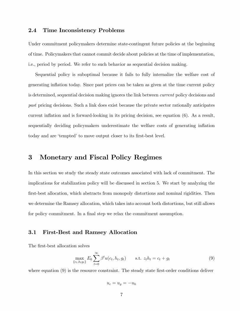
2.4 Time Inconsistency Problems

Under commitment policymakers determine state-contingent future policies at the beginning

of time. Policymakers that cannot commit decide about policies at the time of implementation,

i.e., period by period. We refer to such behavior as sequential decision making.

Sequential policy is suboptimal because it fails to fully internalize the welfare cost of

generating in�ation today. Since past prices can be taken as given at the time current policy

is determined, sequential decision making ignores the link between current policy decisions and

past pricing decisions. Such a link does exist because the private sector rationally anticipates

current in�ation and is forward-looking in its pricing decision, see equation (6). As a result,

sequentially deciding policymakers underestimate the welfare costs of generating in�ation

today and are �tempted�to move output closer to its �rst-best level.

3 Monetary and Fiscal Policy Regimes

In this section we study the steady state outcomes associated with lack of commitment. The

implications for stabilization policy will be discussed in section 5. We start by analyzing the

�rst-best allocation, which abstracts from monopoly distortions and nominal rigidities. Then

we determine the Ramsey allocation, which takes into account both distortions, but still allows

for policy commitment. In a �nal step we relax the commitment assumption.

3.1 First-Best and Ramsey Allocation

The �rst-best allocation solves

maxfct;htgtg

E0

1Xt=0

�tu(ct; ht; gt) s.t. ztht = ct + gt (9)

where equation (9) is the resource constraint. The steady state �rst-order conditions deliver

uc = ug = �uh

7

showing that, given the technological constraints, it is optimal to equate the marginal utility

of private and public consumption to the marginal disutility of labor e¤ort. This simple result

ceases to be optimal in the Ramsey allocation, which takes into account the presence of price

setting and monopoly distortions, as summarized by the implementability constraints (6) and

(7). Speci�cally, the Ramsey allocations solves6

maxfct;ht;�t;Rt�1;gtg

E0

1Xt=0

�tu(ct; ht; gt) (10)

s.t. Equations (6); (7); (8) for all t

Note that the Ramsey allocation still allows for commitment to policies at time zero and full

cooperation between monetary an �scal policymakers. Deriving the �rst order conditions of

(10) and imposing steady state conditions delivers7

� = 1 and R =1

�

as well as the marginal conditions

uc = ��

1 + �uh (11)

ug = �1 + �

1+�q

1 + quh (12)

where q � � chhuhhuh

uccucc

� 0. Equation (11) shows that monopolistic competition creates a

wedge between the marginal utility of private consumption and the marginal disutility of

work. This wedge re�ects the fact that labor fails to receive its marginal product when �rms

have monopoly power, which causes housholds to reduce consumption of produced goods and

to increase consumption of leisure.8

6Since Ricardian equivalence holds we ignore the �nancing decisions of the �scal authority and the initial

debt level R�1B�1, which do not matter for equilibrium determination of the other variables. Since the initial

condition P�1 simply normalizes the implied price level path, it can equally be ignored.7Details of the derivation are in web appendix A.1.8Steady state real wages fall short of their marginal product because w = (1 + �) =� < 1.

8

For uhh < 0, one has q > 0 and equation (12) implies that the optimal level of public

spending falls short of equating the marginal utility of public consumption to the marginal

disutility of work, unlike in the �rst best allocation. One might think that the optimal

provision of public goods should be una¤ected by the presence of a monopolistic mark-up, since

lump sum taxes allow to �nance any price mark-up without generating additional distortions.

However, public spending (and taxes) below the �rst-best level reduce the marginal disutility

of work, which increases the ine¢ ciently low level of private consumption.

3.2 Sequential Policymaking

We now consider separate monetary and �scal authorities that cannot commit to future policy

plans and decide about policies at the time of implementation. To facilitate the exposition,

each policymaker takes as given the current policy choice of the other policymaker, as well

as all future policies and future private-sector choices. We verify the rationality of these

assumptions at the end of this section.

3.2.1 Sequential Fiscal Policy: Spending Bias

Given the assumptions made above, the �scal authority�s problem in period t is

maxfct+j ;ht+j ;�t+j ;gt+jg

Et

1Xj=0

�ju(ct+j; ht+j; gt+j) (13)

s:t: Equations (6); (7); (8) for all t

fct+j; ht+j;�t+j; Rt+j�1 � 1; gt+jg given for j � 1

Eliminating Lagrange multipliers from the �rst order conditions delivers9

ugt = �uhtzt

2�t � 12�t � 1� (�t � 1) (1 + �t + uht

uct

�tzt+ ht

uhhtuct

�tzt)

(FRF)

9Details of the derivation are in web appendix A.2.

9

The �scal authority sets the level of public goods provision gt such that this �scal reaction

function (FRF) is satis�ed, each period.

Consider a steady state in which the in�ation rate is equal to the one chosen by the Ramsey

planner (� = 1). The �scal reaction function then simpli�es to

ug = �uh (14)

showing that �scal policy equates the marginal utility of public consumption to the marginal

disutility of labor e¤ort. While such behavior is consistent with the �rst-best allocation,

it is generally suboptimal in the presence of monopolistic distortions, as argued in section

3.1. Sequential �scal policy thus gives rise to a suboptimally high level of public spending.

This ��scal spending bias�causes the Ramsey allocation to be unattainable in the presence of

sequential �scal policy, because in�ation or �scal spending, or both must deviate from their

Ramsey values. This result is summarized in the following proposition.

Proposition 1 For uhh < 0, sequential �scal policy implies excessive �scal spending in the

presence of price stability.

The economic intuition underlying this result is as follows. By taking future decisions

and the current monetary policy choice Rt as given, the �scal authority considers private

consumption ct to be determined by the Euler equation (7). The �scal authority thus perceives

labor input ht to move one-for-one with government spending gt. In a situation with price

stability, the in�ation costs of public spending are zero (at the margin) and can be ignored,

so that the sequential spending rule (14) appears optimal. When � 6= 1 the marginal costs of

in�ation fail to be zero, leading to the optimality condition FRF.

10

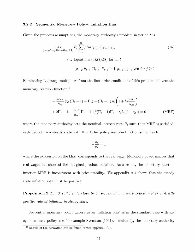
3.2.2 Sequential Monetary Policy: In�ation Bias

Given the previous assumptions, the monetary authority�s problem in period t is

maxfct+j ;ht+j ;�t+j ;Rt+j�1g

Et

1Xj=0

�ju(ct+j; ht+j; gt+j) (15)

s.t. Equations (6),(7),(8) for all t

fct+j; ht+j;�t+j; Rt+j � 1; gt+j�1g given for j � 1

Eliminating Lagrange multipliers from the �rst order conditions of this problem delivers the

monetary reaction function10

� ztuctuht

(�t (�t � 1)� �t)� (�t � 1) �t�1 + ht

uhhtuht

�+ 2�t � 1�

ucctuct(�t � 1) (�(�t � 1)�t � ztht (1 + �t)) = 0 (MRF)

where the monetary authority sets the nominal interest rate Rt such that MRF is satis�ed,

each period. In a steady state with � = 1 this policy reaction function simpli�es to

�ucuh= 1

where the expression on the l.h.s. corresponds to the real wage. Monopoly power implies that

real wages fall short of the marginal product of labor. As a result, the monetary reaction

function MRF is inconsistent with price stability. We appendix A.4 shows that the steady

state in�ation rate must be positive.

Proposition 2 For � su¢ ciently close to 1, sequential monetary policy implies a strictly

positive rate of in�ation in steady state.

Sequential monetary policy generates an �in�ation bias�as in the standard case with ex-

ogenous �scal policy, see for example Svensson (1997). Intuitively, the monetary authority

10Details of the derivation can be found in web appendix A.3.

11

is tempted to stimulate demand by lowering nominal interest rates. Since price adjustments

are costly, the price level will not fully adjust, and real interest rates fall, which stimulates

demand. The real wage increase required to satisfy this additional demand generates in�ation.

3.2.3 Sequential Monetary and Fiscal Policy

We now de�ne a Markov-perfect Nash equilibrium with sequential monetary and �scal policy.

We also verify the rationality of our initial assumptions that sequentially deciding policymakers

can take as given the current policy choice of the other policymaker, as well as all future policies

and future private-sector decisions.

The private sector�s optimality conditions (6) and (7), the feasibility constraint (8), as well

as the policy reactions functions FRF and MRF, all depend on current and future variables

only. This observation suggests the existence of an equilibrium where current play is a func-

tion of the current exogenous variables zt and �t only. Future play then depends on future

exogenous variables only, which justi�es the assumption that future equilibrium play (and

o¤-equilibrium play) is independent of current play. If each period, in addition, monetary

and �scal policy are determined simultaneously, Nash equilibrium requires taking the other

player�s current decision as given. This justi�es the assumptions made in deriving FRF and

MRF and motivates the following de�nition.

De�nition 3 (SP) A stationary Markov-perfect Nash equilibrium with sequential monetary

and �scal policy consists of time-invariant policy functions c(zt; �t); h(zt; �t); �(zt; �t); R(zt; �t);

g(zt; �t) solving equations (6),(7),(8), FRF and MRF.

We now show that Stackelberg leadership by one of the policy authorities (with regard

to the within-period moves) is consistent with the same equilibrium outcome. While the

policy problem of the Stackelberg follower remains unchanged, the Stackelberg leader takes

into account the reaction function of the follower. Yet, the Lagrange multipliers associated

12

with additionally imposing MRF in the sequential �scal problem (13) or with imposing FRF

in the sequential monetary problem (15) are zero. These reaction functions can be derived

from the �rst order conditions of the leader�s policy problem even when the follower�s reaction

function is not being imposed.

Intuitively, the leadership structure does not matter for the equilibrium outcome because

both authorities are pursuing the same policy objective. Any departure from the Ramsey solu-

tion is thus entirely due to sequential decision making. The presence of distinct policymakers

and the sequence of moves will matter in section 5 when we consider a monetary authority

that is more in�ation averse than the �scal authority.

4 How Much In�ation is Optimal?

We have shown that a steady state with sequential monetary and �scal policy (SP) involves

positive rates of in�ation (proposition 2). We now show that price stability (� = 1) is

not optimal whenever �scal policy faces a commitment problem, i.e., is described by FRF.

Monetary policy should then aim at positive rates of in�ation because this increases the

perceived costs of public spending for the �scal authority and reduces the �scal spending

bias. This leads to a �rst order welfare gain11, while the costs of locally deviating from price

stability are of second order only. This is formally shown in web appendix A.5:

Proposition 4 Assume uhh < 0. In a steady state with sequential �scal policy, welfare in-

creases and �scal spending decreases with the steady state in�ation rate, locally at � = 1.

11This is so because with sequential �scal policy uc > ug = �uh when � = 1, see FRF.

13

What is then the welfare maximizing in�ation rate that correctly internalizes the sequential

�scal policy distortion? This in�ation rate can be obtained as the solution to the problem

maxfct;ht;�t;Rt�1;gtg

E0

1Xt=0

�tu(ct; ht; gt) (OI)

s.t. Equations (6),(7),(8),(FRF) for all t

where monetary policy can commit, while �scal behavior is described by FRF. We will refer to

this situation as the optimal in�ation (OI) regime. If the optimal steady state in�ation rate is

below (above) the rate emerging in the steady state of the Markov-perfect Nash equilibrium,

then an in�ation conservative (liberal) central banker would appear desirable.12

4.1 Quantifying the Policy Biases

In this section we quantify the steady state under sequential monetary and �scal policy (SP)

and compare it to the Ramsey allocation and also to the allocation achieved under the optimal

in�ation (OI) regime.

We consider the following preference speci�cation, which is consistent with balanced

growth,

u(ct; ht; gt) = log (ct)� !hh1+'t

1 + '+ !g log (gt) (16)

with !h > 0, !g � 0 and ' � 0. As a baseline calibration, we set � = 0:9913 implying an

annual real interest rate of 3:5%. The steady state price elasticity of demand � is set at �6,

so that there is a 20% mark-up over marginal costs. The degree of price stickiness � is chosen

to be 17:5, such that the log-linearized version of the Phillips curve (6) is consistent with the

one in Schmitt-Grohé and Uribe (2004). Labor supply elasticity is set to '�1 = 1 and the

utility weights !h and !g are chosen such that in the Ramsey steady state agents work 20%

12Since steady state in�ation depends on steady state nominal interest rates only, see equation (7), the

optimal in�ation rate implicitly determines optimal monetary policy.

14

of their time (h = 0:2) and spend 20% of output on public goods (g = 0:04).13

We tested the robustness of our numerical results by considering a wide range of alternative

model parameterizations and by using di¤erent starting values.14 The baseline results are

robust, except for the �exible price limit (� ! 0) and for inelastic labor supply (large '). In

both cases the time-inconsistency problems of policy disappear and the real allocations under

SP approach the Ramsey steady state.

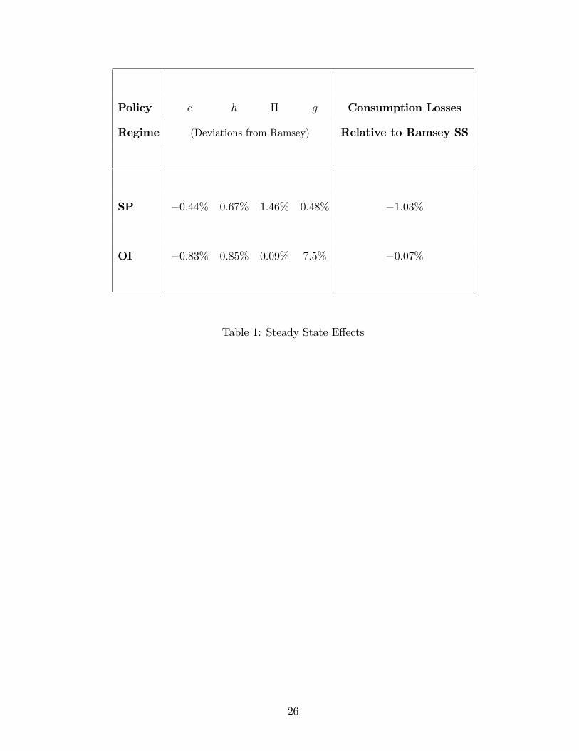
The �rst row of table 1 presents information on the steady state in the SP regime. All

variables are expressed as percentage deviations from their corresponding Ramsey steady state

values.15 The last column of the table reports the steady state welfare loss, expressed in terms

of the permanent reduction in private consumption making the Ramsey steady state welfare

equivalent to the considered policy regime.16 In line with proposition 2, the sequential policy

outcome is characterized by an in�ation bias, which turns out to be sizable. In addition, there

is a small �scal spending bias. Overall, the welfare losses generated by the sequential conduct

of policy are fairly large, in the order of 1% of steady state consumption per period.

The second row of table 1 shows the outcome under the OI regime. The optimal in�ation

rate is not only lower than the in�ation rate in the SP regime but also very close to price

stability. As suggested by proposition 4, reducing in�ation from the level of the SP regime

to the optimal level increases the �scal spending bias. While the �scal spending increase is

fairly large, the optimal in�ation rate nevertheless eliminates large part of the welfare losses

associated with the SP regime. This suggests that the �scal spending bias, despite being

13This requires !h = 26:042 and !g = 0:227, see equations (44) and (45), in web appendix A.6.14To keep the Ramsey steady state invariant to the parmeterization, we adjusted the weights !h and !g.

We used di¤erent starting values to test for multiplicities in the steady state, as occurred in King and Wolman

(2004), and did not ecounter any, possibly due to the fact that in our setting the private sector takes all of its

decisions after policy has been determined.15In the Ramsey steady state c = 0:16, h = 0:2, g = 0:04 and � = 1.16Web appendix A.8 explains the computation of the welfare losses.

15

sizable in absolute value, is not very detrimental in welfare terms. Clearly, this result hinges

partly on the availability of lump sum taxes.

The results from table 1 show that the optimal in�ation rate is well below the one emerging

in the SP regime. This holds for a wide range of alternative model parameterizations, which

suggests that installing a conservative monetary authority should be desirable on welfare

grounds whenever sequential �scal policy is described by FRF.

5 Conservative Monetary Authority

This section analyzes whether the distortions stemming from sequential monetary and �scal

policy decisions can be reduced by installing a monetary authority that is more in�ation

averse than society. Rogo¤ (1985) and Svensson (1997) have shown this to be the case if �scal

policy is treated as exogenous. Following Rogo¤ (1985), we consider a �weight conservative�

monetary authority with period utility function

(1� �)u(ct+j; ht+j; gt+j)� �(�t+j � 1)2

2

where � 2 [0; 1] is a measure of monetary conservatism. For � > 0 the monetary authority

dislikes in�ation (and de�ation) more than society; if � = 1 the policymaker cares about

in�ation only. The preferences of the �scal authority remain unchanged.

With monetary and �scal authorities now pursuing di¤erent policy objectives, the equi-

librium outcome will depend on the timing of policy moves, i.e., on whether �scal policy is

determined before, after, or simultaneously with monetary policy each period. Casual obser-

vation suggests that it takes longer to enact �scal decisions, which would imply that �scal

policy is determined before monetary policy. At the same time, the time lag between a mon-

etary policy decision and its e¤ects on the economy may be substantial too. It thus remains

to be ascertained which of these timing structures is the most relevant for actual economies.

16

For these reasons, we consider Nash as well as leadership equilibria.

5.1 Nash and Leadership Equilibria

This section de�nes the various Markov-perfect equilibria in the presence of a conservative

monetary authority. As it turns out, the equilibrium outcomes with simultaneous monetary

and �scal decisions each period (Nash case) and with monetary policy determined before

�scal policy each period (monetary leadership) are very similar. This similarity emerges

because in both cases �scal policy takes current monetary decisions as given, so that �scal

policy continues to be described by FRF, i.e., by the reaction function in the absence of a

conservative authority. For space constraints we therefore only discuss the Nash case.

The situation in which �scal policy is determined before monetary policy (�scal leadership)

di¤ers considerably. The �scal authority has to take into account the conservative monetary

authority�s within-period reaction function. Monetary policy can then use �o¤-equilibrium�

behavior to discipline the behavior of the �scal authority along the equilibrium path. Fiscal

leadership thus opens the possibility for outcomes that are welfare superior to those achieved

in the OI regime.

First, consider the case with simultaneous decisions. While the policy problem of the �scal

authority remains unchanged, the monetary authority now solves

maxfct+j ;ht+j ;�t+j ;Rt+j�1g

Et

1Xj=0

�j�(1� �)u(ct+j; ht+j; gt+j)�

�

2(�t+j � 1)2

�(17)

s.t. Equations (6),(7),(8) for all t

fct+j; ht+j;�t+j; Rt+j � 1; gt+j�1g given for j � 1

Taking �rst order conditions of problem (17) and eliminating Lagrange multipliers delivers

the conservative monetary authority�s reaction function that we denote by CMRF.17 For

17Web appendix A.9 provides the technical details. As before, CMRF implies that current interest rates

17

� = 0, CMRF reduces to the monetary reaction function without conservatism (MRF). This

motivates the following de�nition.

De�nition 5 (CSP-Nash) A stationary Markov-perfect Nash equilibrium with sequential

and conservative monetary policy, sequential �scal policy, and simultaneous policy decisions

consists of policy functions c(zt; �t); h(zt; �t); �(zt; �t); R(zt; �t); g(zt; �t) solving equations (6),

(7), (8), FRF and CMRF.

Next, consider the case of �scal leadership (FL). The �scal authority must now take into

account the conservative monetary reaction function (CMRF). The �scal authority�s policy

problem at time t is thus given by

maxfct+j ;ht+j ;�t+j ;Rt+j�1;gt+jg

Et

1Xj=0

�ju(ct+j; ht+j; gt+j) (18)

s.t. Equations (6),(7),(8), CMRF for all t

fct+j; ht+j;�t+j; Rt+j � 1; gt+jg given for j � 1

The �rst order conditions associated with problem (18) deliver the corresponding �scal reac-

tion function that we denote by CFRF-FL. We propose the following de�nition.

De�nition 6 (CSP-FL) A stationary Markov-perfect equilibrium with sequential and con-

servative monetary policy, sequential �scal policy, and �scal policy deciding before monetary

policy, consists of policy functions c(zt; �t); h(zt; �t); �(zt; �t); R(zt; �t); g(zt; �t) solving equa-

tions (6), (7), (8), CFRF-FL and CMRF.

depend on current economic conditions only, validating the conjecture in (17) that in a Markov-perfect equi-

librium future policy choices can be taken as given.

18

5.2 Steady State Implications

We now determine the steady state properties for the various timing arrangements with an

in�ation conservative central banker. Our �rst result is that �scal leadership in combination

with a fully conservative monetary authority achieves the Ramsey steady state.

Proposition 7 The Ramsey steady state is consistent with sequential policymaking in a regime

with �scal leadership, if the monetary authority is fully conservative (� = 1).

Intuitively, with �scal leadership the �scal authority anticipates the within-period reaction

of the monetary authority. In particular, for � = 1 the monetary authority is determined

to achieve price stability at all costs. A �scal expansion above the Ramsey spending level

generates in�ationary pressures and thus triggers an increase in interest rates to restrain

private consumption. The �scal authority therefore internalizes that �scal spending crowds

out private consumption one-for-one. This e¤ect disciplines �scal spending and allows the

achievement of the Ramsey steady state despite sequential policymaking by both authorities.

A formal proof is provided in web appendix A.10. The next proposition shows that this fails

to be possible with other timing arrangements:

Proposition 8 For uhh < 0, the Ramsey steady state cannot be achieved with sequential

policymaking in a regime with monetary leadership or simultaneous decisions, for any degree

of monetary conservatism.

With monetary leadership or simultaneous decisions, the behavior of the �scal authority

continues to be described by the �scal reaction function (FRF). It then follows from proposi-

tion 1 that in�ation or �scal spending, or both, must deviate from their Ramsey steady state

values. Nevertheless, the quantitative �ndings from section 4.1 suggest that a conservative

monetary authority should remain desirable.

19

Figure 1 illustrates this point using the baseline calibration of section 4.1. The �gure

displays the consumption equivalent steady state welfare losses associated with intermediate

degrees of monetary conservatism � 2 [0; 1] relative to the Ramsey steady state. The upper

horizontal line indicates the welfare losses of the OI regime. Note that in the Nash case a fully

conservative monetary authority (� = 1) approximately achieves the steady state welfare level

of the OI regime.18 Thus, even in the absence of �scal leadership large part of the welfare losses

associated with sequential monetary and �scal policy can be recovered through a su¢ cient

degree of monetary conservatism.

Using again the baseline calibration, �gure 2 illustrates how the steady state values of

private consumption, labor e¤ort, in�ation and public spending depend on the degree of

monetary conservatism. While an increase in monetary conservatism reduces the in�ation

bias for all timing protocols, its e¤ect on the �scal spending bias depends on whether �scal

policy anticipates the monetary policy reaction. If �scal policy takes monetary decisions as

given, monetary conservatism results in an increased �scal spending bias, as suggested by

proposition 4. Nevertheless, an in�ation conservative central banker remains desirable, as a

value of � slightly below 1 recovers the OI outcome.

5.3 Implications for Stabilization Policy

This section extends the analysis to a stochastic economy, considering stabilization policy

in response to technology and mark-up shocks. We restrict attention to the sequential pol-

icy regime that achieves the Ramsey steady state, i.e., �scal leadership and full monetary

conservatism (� = 1).

Full monetary conservatism implies that the central bank will achieve stable prices at all

times. Thus, a necessary condition for the optimality of the impulse response under this policy

18The welfare level of the OI regime is achieved by a value of � very close but slightly below 1.

20

arrangement is that the Ramsey allocation can be achieved with a stable price path. The next

proposition states that this is also a su¢ cient condition.19

Proposition 9 If the Ramsey response to shocks can be achieved with a stable path for prices,

then it is consistent with sequential policymaking in a regime with �scal leadership and fully

conservative monetary policy (� = 1).

The following proposition provides su¢ cient conditions under which the Ramsey impulse

response to shocks involves a stable price path.

Proposition 10 Assume preferences over ct; ht; and gt are of the constant relative risk class.

If private and public consumption have the same relative risk aversion, then the Ramsey

response to a technology shock involves no deviation from price stability.

The proof is given in web appendix A.12 and shows that price stability under Ramsey

policy requires a stable private consumption to output ratio, as well as a stable public con-

sumption to output ratio. Maintaining both ratios constant is not possible if preferences are

not homogeneous in (ct; gt). Thus, the Ramsey response to technology shocks will generally

involve deviations from price stability.

The Ramsey response to mark-up shocks will equally involve deviations from price stability.

This is the case even when the assumptions of proposition 10 are satis�ed. We illustrate this

point in �gure 3 for the baseline parameterization of section 4.1 and a positive mark-up

shock of three standard deviations.20 The Ramsey response involves an initial rise in in�ation

followed by a small but persistent amount of de�ation, while the sequential policy implements

19The proof is given in web appendix A.11 and shows that the �rst order conditions of the Ramsey problem

with stable prices are identical to the equilibrium conditions implied by �scal leadership and full conservatism.20Following Ireland (2004) we set the quarterly autocorrelation of mark-up shocks to �n = 0:96. We choose

Ireland�s estimate of the standard deviations of innovations, which requires multiplying the value reported in

his table 1 by the price adjustment parameter �.

21

stable prices at all times. Overall, the deviations from price stability in the Ramsey regime

seem small (in the order of less than 0.1% per quarter) and the responses di¤er across regimes

only for the early periods following a shock.

Although the stabilization policy associated with �scal leadership and full monetary conser-

vatism is not fully optimal, the following proposition suggests that such a policy arrangement

remains close to fully optimal:

Proposition 11 Sequential policymaking in a regime with �scal leadership and fully conserv-

ative monetary policy (� = 1) is consistent with the Ramsey response to shocks under �exible

prices.

The proof is given in web appendix A.13. Thus, �scal leadership and full conservatism

eliminate all gaps to the Ramsey equilibrium with �exible prices. The presence of sticky

prices allows, however, to improve somewhat upon the �exible price allocation, see Adao et

al. (2003). Since these gains are likely to be small, full monetary conservatism achieves

desirable stabilization outcomes in a setting with �scal leadership.

6 Distortionary Taxation

The discussion so far relied on the availability of lump sum taxes. While this assumption allows

to derive the main results analytically, it also implies that the government could potentially

eliminate the monopolistic distortion, and thereby the commitment problem, via an output

subsidy to �rms or a wage subsidy to workers.

In a companion note, Adam and Billi (2008), we assume that �scal spending must be

�nanced by distortionary labor income taxes. We �nd again that sequential monetary policy

gives rise to a steady state in�ation bias and that sequential �scal policy results in overspending

on public goods whenever prices are stable. Numerical exercises suggest that these policy

22

biases are considerably larger than in a setting with lump sum taxes: with the sequential �scal

authority not fully internalizing the cost of public spending and taxation, more overspending

implies higher labor taxes, thereby lower output, and thus even stronger incentives to increase

public spending and in�ation.

When numerically evaluating the e¤ects of monetary conservatism, we �nd again that

�scal leadership with fully conservative monetary policy achieves the Ramsey steady state,

and close to full monetary conservatism is optimal for the other timing protocols. Monetary

conservatism thus remains desirable in a setting with distortionary taxes.

7 Conclusions

This paper analyzes the policy biases stemming from sequential monetary and �scal policy-

making, asking whether an in�ation conservative central banker remains desirable in a setting

with endogenous �scal policy.

While the lack of �scal commitment can make it optimal to aim for positive in�ation rates,

the optimal deviations from price stability turn out to be quantitatively small. Since lack of

monetary commitment generates too much in�ation, installing a conservative central banker

remains welfare improving when �scal policy is endogenous.

In a setting with �scal leadership, arguably the most relevant case, installing a fully con-

servative central bank which focuses exclusively on stabilizing in�ation eliminates not only

the in�ation bias but also the �scal spending bias in steady state. The case for monetary

conservatism may thus be even stronger in a setting with endogenous �scal policy.

23

References

Adam, K., and R. Billi (2008): �Monetary Conservatism and Fiscal Policy: The Case of

Distortionary Taxes,�University of Mannheim Mimeo.

Adão, B., I. Correia, and P. Teles (2003): �Gaps and Triangles,�Review of Economic

Studies, 70, 699�713.

Barro, R., and D. B. Gordon (1983): �A Positive Theory of Monetary Policy in a Natural

Rate Model,�Journal of Political Economy, 91, 589�610.

Chari, V. V., and P. J. Kehoe (1990): �Sustainable Plans,�Journal of Political Economy,

98, 783�802.

Ireland, P. (2004): �Technology Shocks in the New Keynesian Model,�Review of Economics

and Statistics, 86(4), 923�936.

King, R. G., and A. L. Wolman (2004): �Monetary Discretion, Pricing Complementarity

and Dynamic Multiple Equilibria,�Quarterly Journal of Economics, 119(4), 1513�1553.

Klein, P., P. Krusell, and J.-V. Ríos-Rull (2008): �Time Consistent Public Policy,�

Review of Economic Studies, 75, 789�808.

Kydland, F. E., and E. C. Prescott (1977): �Rules Rather Than Discretion: The

Inconsistency of Optimal Plans,�Journal of Political Economy, 85, 473�492.

Leeper, E. M. (1991): �Equilibria under Active and Passive Monetary and Fiscal Policies,�

Journal of Monetary Economics, 27, 129�147.

Lucas, R. E., and N. L. Stokey (1983): �Optimal Fiscal and Monetary Policy in an

Economy Without Capital,�Journal of Monetary Economics, 12, 55�93.

24

Maskin, E., and J. Tirole (2001): �Markov Perfect Equilibrium: I. Observable Actions,�

Journal of Economic Theory, 100, 191�219.

Rogoff, K. (1985): �The Optimal Degree of Commitment to an Intermediate Monetary

Target,�Quarterly Journal of Economics, 100(4), 1169�89.

Rotemberg, J. J. (1982): �Sticky Prices in the United States,�Journal of Political Econ-

omy, 90, 1187�1211.

Schmitt-Grohé, S., and M. Uribe (2004): �Optimal Fiscal and Monetary Policy under

Sticky Prices,�Journal of Economic Theory, 114(2), 198�230.

Svensson, L. E. O. (1997): �Optimal In�ation Targets, �Conservative�Central Banks, and

Linear In�ation Contracts,�American Economic Review, 87, 98�114.

Walsh, C. E. (1995): �Optimal Contracts for Central Bankers,�American Economic Review,

85, 150�67.

Woodford, M. (1998): �Doing Without Money: Controlling In�ation in a Post-Monetary

World,�Review of Economic Dynamics, 1, 173�209.

(2003): Interest and Prices. Princeton University Press, Princeton.

25

Policy c h � g Consumption Losses

Regime (Deviations from Ramsey) Relative to Ramsey SS

SP �0:44% 0:67% 1:46% 0:48% �1:03%

OI �0:83% 0:85% 0:09% 7:5% �0:07%

Table 1: Steady State E¤ects

26

0 0.1 0.2 0.3 0.4 0.5 0.6 0.7 0.8 0.9 1­1.2

­1

­0.8

­0.6

­0.4

­0.2

0Consumption Losses Relative to Ramsey SS

Degree of Conservatism (Alpha)

Per

cent

age 

Poi

nts

OICSP­FLCSP­Nash

Figure 1: Welfare Gains From Monetary Conservatism

27

0 0.2 0.4 0.6 0.8 1

­0.8

­0.7

­0.6

­0.5

­0.4

­0.3

­0.2

­0.1

0Private Consumption

Degree of Conservatism (Alpha)

Dev

iatio

n fro

m R

amse

y %

OICSP­FLCSP­Nash

0 0.2 0.4 0.6 0.8 10

0.1

0.2

0.3

0.4

0.5

0.6

0.7

0.8

Labor Effort

Degree of Conservatism (Alpha)

Dev

iatio

n fro

m R

amse

y %

OICSP­FLCSP­Nash

0 0.2 0.4 0.6 0.8 10

0.2

0.4

0.6

0.8

1

1.2

1.4

Gross Inflation

Degree of Conservatism (Alpha)

Dev

iatio

n fro

m R

amse

y %

OICSP­FLCSP­Nash

0 0.2 0.4 0.6 0.8 10

1

2

3

4

5

6

7

Public Goods

Degree of Conservatism (Alpha)

Dev

iatio

n fro

m R

amse

y %

OICSP­FLCSP­Nash

Figure 2: Steady State E¤ects of Monetary Conservatism

28

0 2 4 6 8 10 12 14 16 18 20­0.5­0.4­0.3­0.2­0.1

0Mark­Up Shock

Priv

ate 

Con

s.RamseyCSP­FL (Alpha=1)

0 2 4 6 8 10 12 14 16 18 20­0.5­0.4­0.3­0.2­0.1

0

Labo

r Effo

rt

0 2 4 6 8 10 12 14 16 18 20­0.05

0

0.05

0.1

Gro

ss In

flatio

n

0 2 4 6 8 10 12 14 16 18 20­0.1

­0.05

0

0.05

0.1

Publ

ic G

oods

Quarters

Figure 3: Responses to Mark-Up Shocks and Monetary Conservatism

29

A Web Appendix - NOT FOR PUBLICATION

A.1 Ramsey Steady State

The Lagrangian of the Ramsey problem (10) is

maxfct;ht;�t;Rt;gtg

E0

1Xt=0

�tnu(ct; ht; gt)

+ 1t

�uct(�t � 1)�t �

uctztht�

�1 + �t +

uhtuct

�tzt

�� �uct+1(�t+1 � 1)�t+1

�+ 2t

�uctRt� �uct+1

�t+1

�+ 3t

�ztht � ct �

�

2(�t � 1)2 � gt

��The �rst-order conditions w.r.t. (ct; ht;�t; Rt; gt), respectively, are given by

uct + 1t

�ucct(�t � 1)�t �

ucctztht�

(1 + �t)

�� 1t�1ucct(�t � 1)�t + 2t

ucctRt

� 2t�1ucct�t

� 3t = 0 (19)

uht � 1tuctzt�

�1 + �t +

uhtuct

�tzt+ ht

uhhtuct

�tzt

�+ 3t zt = 0 (20)

� 1t � 1t�1

�uct(2�t � 1) + 2t�1

uct�2t� 3t �(�t � 1) = 0 (21)

� 2tuctR2t

= 0 (22)

ugt � 3t = 0 (23)

where j�1 = 0 for j = 1; 2. We denote the Ramsey steady state by dropping time subscripts.

Equation (22), uct > 0 and Rt � 1 imply

2 = 0

Equations (23) delivers

3 = ug > 0

30

This and (21) gives

� = 1

From (7) it then follows

R =1

�

Then (6) delivers

1 + � +uhuc� = 0 (24)

This delivers (11) shown in the main text. Using the previous results, (20) simpli�es to

uh � 1h

�uhh� + ug = 0 (25)

From (19) one obtains

1h

�=

uc � ugucc (1 + �)

(26)

Substituting (26) into (25) delivers

uh �uc � ugucc (1 + �)

uhh� + ug = 0

Using (24) to substitute for uc one gets

ug = �uh1 +

��1+�

�2uhhucc

1 + �1+�

uhhucc

Using (24) again to substitute �1+�

delivers (12) shown in the main text.

31

A.2 Sequential Fiscal Reaction Function

The �scal problem (13) is

maxfct+j ;ht+j ;�t+j ;gt+jg

Et

1Xj=0

�jnu(ct+j; ht+j; gt+j)

+ 1t+j

�uct+j(�t+j � 1)�t+j �

uct+jzt+jht+j�

�1 + �t+j +

uht+juct+j

�t+jzt+j

�� �uct+j+1(�t+j+1 � 1)�t+j+1

i+ 2t+j

�uct+jRt+j

� �uct+j+1�t+j+1

�+ 3t+j

�zt+jht+j � ct+j �

�

2(�t+j � 1)2 � gt+j

��taking as given Rt+j�1 and other variables dated t + j for j � 1. The �rst order conditions

w.r.t. (ct; ht;�t; gt), respectively, are given by

uct + 1t

�ucct(�t � 1)�t �

ucctztht�

(1 + �t)

�+ 2t

ucctRt

� 3t = 0 (27)

uht � 1tuctzt�

�1 + �t +

uhtuct

�tzt+ ht

uhhtuct

�tzt

�+ 3t zt = 0 (28)

1t uct(2�t � 1)� 3t �(�t � 1) = 0 (29)

ugt � 3t = 0 (30)

From (29) and (30) one gets

1t =ugt�(�t � 1)uct(2�t � 1)

Using the previous result and (30) to substitute the Lagrange multipliers in (28) delivers FRF

shown in the main text.

32

A.3 Sequential Monetary Reaction Function

The monetary problem (15) is

maxfct+j ;ht+j ;�t+j ;Rt+jg

Et

1Xj=0

�jnu(ct+j; ht+j; gt+j)

+ 1t+j

�uct+j(�t+j � 1)�t+j �

uct+jzt+jht+j�

�1 + �t+j +

uht+juct+j

�t+jzt+j

�� �uct+j+1(�t+j+1 � 1)�t+j+1

i+ 2t+j

�uct+jRt+j

� �uct+j+1�t+j+1

�+ 3t+j

�zt+jht+j � ct+j �

�

2(�t+j � 1)2 � gt+j

��taking as given gt+j�1 and other variables dated t + j for j � 1. The �rst order conditions

w.r.t. (ct; ht;�t; Rt), respectively, are given by

uct + 1t

�ucct(�t � 1)�t �

ucctztht�

(1 + �t)

�+ 2t

ucctRt

� 3t = 0 (31)

uht � 1tuctzt�

�1 + �t +

uhtuct

�tzt+ ht

uhhtuct

�tzt

�+ 3t zt = 0 (32)

1t uct(2�t � 1)� 3t �(�t � 1) = 0 (33)

� 2tuctR2t

= 0 (34)

Equation (34), uct > 0 and Rt � 1 imply

2t = 0

Then solving (31), (32) and (33) for 3t delivers, respectively,

3t = uct + 1t

�ucct(�t � 1)�t �

ucctztht�

(1 + �t)

�(35)

3t = �uhtzt+ 1t

uct�

�1 + �t +

uhtuct

�tzt+ ht

uhhtuct

�tzt

�(36)

3t = 1t

uct (2�t � 1)� (�t � 1)

(37)

33

Equations (35) and (37) imply

1t =�

2�t�1�t�1 �

ucctuct(�(�t � 1)�t � ztht (1 + �t))

(38)

While (36) and (37) give

1t =�

ztuctuht

�1 + �t � 2�t�1

�t�1 +uhtuct

�tzt+ ht

uhhtuct

�tzt

� (39)

From (38) and (39) one obtains MRF shown in the main text.

A.4 Proof of Proposition 2

We �rst show that MRF cannot hold in the neighborhood of � = 1. In steady state one can

rewrite MRF as

�

�1 +

ucuh

�+O(�� 1) = 0 (40)

where O(��1) summarizes terms that converge to zero as (�� 1)! 0. In a steady state with

� = 1 equation (6) delivers ucuh< � �

1+�< �1. Since the implicit function uc

uh(�) de�ned by (6)

exists, this implies that ucuhis bounded away from �1 also in a su¢ ciently small neighborhood

around � = 1. Thus, (40) cannot hold in the neighborhood of � = 1. Moreover, from R � 1

and (7) we have � � � in steady state. For � su¢ ciently close to 1, it then follows that MRF

can only hold if � > 1.

A.5 Proof of Proposition 4

The e¤ect of in�ation on steady state utility is given by

du

d�= uc

@c

@�+ uh

@h

@�+ ug

@g

@�(41)

where c(�); h(�); g(�) denote the steady state levels emerging under sequential �scal policy

when monetary policy implements in�ation rate �, and the derivatives uj (j = c; h; g) are

34

evaluated at this steady state. We �rst evaluate (41) at � = 1. Equation (6) delivers

uc = ��

1 + �uh (42)

Totally di¤erentiating (8) and evaluating at � = 1 gives

@c

@�=@h

@�� @g

@�

Using this result and (14), then (41) can be rewritten as

du

d�= (uc � ug)

@c

@�

Equations (14) and (42) imply uc > ug, thus

sign

�du

d�

�= sign

�@c

@�

�(43)

To determine the sign of @c=@� we totally di¤erentiate FRF, (6), and (8) and evaluate at

� = 1, this delivers0BBBBB@0 �uhh �ugg

h�� uhucc

u2c�h�� uhhuc

0

�1 1 �1

1CCCCCA

0BBBBB@@c@�

@h@�

@g@�

1CCCCCA =

0BBBBB@h� uhuhh

uc

0

0

1CCCCCASolving for @c

@�and @g

@�gives

@c

@�=

ucuhhucuhhugg � uccuhugg � uccuhuhh

h�uhuhhuc

@g

@�=

�ucuhh + uccuhucuhhugg � uccuhugg � uccuhuhh

h�uhuhhuc

When uhh < 0, signing these expression delivers @c@�> 0 and @g

@�< 0, as claimed. The former

inequality and (43) imply dud�> 0, locally at � = 1.

35

A.6 Utility Weights

For the period utility speci�cation (16), the Ramsey policy marginal conditions (11) and (12),

respectively, deliver

!h =1

ch'1 + �

�(44)

!g = !hgh'1 + �

1+�ch'

1 + ch'

(45)

A.7 Solving for the Equilibrium with Sequential Monetary and Fis-

cal Policy

We show how to solve for the stochastic Markov-perfect Nash equilibrium with sequential

monetary and �scal policy. We illustrate the method for the SP case, i.e., without a conserva-

tive central banker, but the method readily extends to the case with a conservative monetary

authority. The Markov perfect Nash equilibrium solves the following problem

maxfct+j ;ht+j ;�t+j ;Rt+j ;gt+jg

Et

1Xj=0

�ju(ct+j; ht+j; gt+j) (46)

s.t.

Equations (6),(7),(8) for all t

Et (ct+j; ht+j;�t+j; Rt+j; gt+j) given for j � 1

One should note that FRF and MRF need not be imposed, since they can already be derived

from the �rst order conditions of this problem, see sections 3.2.1 and 3.2.2, respectively. The

solution of problem (46) will always satisfy FRF and MRF.

36

Then, the recursive formulation of the Lagrangian of problem (46) is

W (zt; �t) = min( 1t ; 2t ; 3t )

max(ct;ht;�t;Rt;gt)

ff (�) + �EtW (zt+1; �t+1)g (47)

s.t.

zt+1 = (1� �z) + �zzt + "zt+1

�t+1 = � (1� ��) + ���t + "�t+1

where the one-period return is

f (�) = u(ct; ht; gt)

+ 1t

�uct(�t � 1)�t �

uctztht�

�1 + �t +

uhtuct

�tzt

�� EASt

�+ 2t

�uctRt� EISt

�+ 3t

�ztht � ct �

�

2(�t � 1)2 � gt

�with the expectations functions

EASt � �Etuct+1(�t+1 � 1)�t+1 (48)

EISt � �Etuct+1�t+1

(49)

taken as given. The additional control variables 1t , 2t ,

3t are the Lagrange multipliers of the

implementability constraints (6) and (7), and the feasibility constraint (8), respectively.

We then solve for the steady state using the �rst order conditions of the recursive formu-

lation (47). Thereafter, we compute a quadratic approximation of the one-period return f(�)

around this steady state. This step involves quadratically approximating the implementabil-

ity and feasibility constraints. Instead, the expectation functions EASt and EISt are linearly

approximated as

EASt � a10 + a11 (zt � 1) + a12 (�t � �) (50)

EISt � a20 + a21 (zt � 1) + a22 (�t � �) (51)

37

Importantly, postulating linear expectation functions is su¢ cient to obtain a �rst order ap-

proximation to the equilibrium dynamics and policy functions. The policymaker takes expec-

tations functions as given, therefore, they do not show up in di¤erentiated form in the �rst

order conditions. Moreover, linear expectations functions are su¢ cient to evaluate the La-

grangian, i.e., utility, up to second order. This is the case because either the implementability

constraints or the Lagrange multipliers are zero in a su¢ ciently small neighborhood around

the steady state. As a result, no �rst order terms appear when evaluating the quadratic ap-

proximation of f(�) at the solution. Obviously, this is just a restatement of the fact that (47)

is an unconstrained optimization problem.

We now explain how we compute the expectation functions (50) and (51). We start with

an initial guess for aji (j = 1; 2; i = 0; 1; 2), then we solve (47) with f(�) replaced by its

quadratic approximation. We update �ji , as explained below, and continue iterating until the

maximum absolute change of the policy functions drops below the square root of machine

precision, i.e., 1:49 � 10�8.

Let the solution for the policy functions c (�) and �(�) be given by

ct+1 � c = �cz (zt+1 � 1) + �c� (�t+1 � �) (52)

�t+1 � � = ��z (zt+1 � 1) + ��� (�t+1 � �) (53)

where variables without time subscript denote steady state values. A �rst-order approximation

of the expectation functions (48) and (49) then delivers

EASt � EASt��ss+@EASt@ct+1

����ss

Et (ct+1 � c) +@EASt@�t+1

����ss

Et (�t+1 � �)

EISt � EISt��ss+@EISt@ct+1

����ss

Et (ct+1 � c) +@EISt@�t+1

����ss

Et (�t+1 � �)

where jss indicates expressions evaluated at steady state. These conditions together with (52),

38

(53) and

Et (zt+1 � 1) = �z (zt � 1)

Et (�t+1 � �) = �� (�t � �)

deliver the expectations functions consistent with the approximated policy functions

a10 = �uc(�� 1)�

a11 = ��z [(�� 1)�ucc�cz + uc(2�� 1)��z]

a12 = ��� [(�� 1)�ucc�c� + uc(2�� 1)���]

a20 = �uc�

a21 = ��z�

�ucc�cz � uc

���z�

a22 = ����

�ucc�c� � uc

�����

A.8 Consumption Losses Relative to Ramsey

Let u (c; h; g) denote the period utility for the Ramsey steady state and let u�cA; hA; gA

�represent the period utility for the steady state of an alternative policy regime. The permanent

reduction in private consumption that would imply the Ramsey steady state to be welfare

equivalent to the alternative policy regime �A � 0 is implicitly de�ned by

1

1� �u�cA; hA; gA

�=

1

1� �u�c(1 + �A); h; g

�=

1

1� ��u (c; h; g) + log

�1 + �A

��where the second equality uses equation (16). Therefore, one obtains

�A = exp�u�cA; hA; gA

�� u (c; h; g)

�� 1

39

A.9 Conservative Monetary Reaction Function

The conservative monetary problem (17) is

maxfct+j ;ht+j ;�t+j ;Rt+jg

Et

1Xj=0

�jn(1� �)u(ct+j; ht+j; gt+j)�

�

2(�t+j � 1)2

+ 1t+j

�uct+j(�t+j � 1)�t+j �

uct+jzt+jht+j�

�1 + �t+j +

uht+juct+j

�t+jzt+j

�� �uct+j+1(�t+j+1 � 1)�t+j+1

i+ 2t+j

�uct+jRt+j

� �uct+j+1�t+j+1

�+ 3t+j

�zt+jht+j � ct+j �

�

2(�t+j � 1)2 � gt+j

��taking as given gt+j�1 and variables dated t + j for j � 1. The �rst order conditions w.r.t.

(ct; ht;�t; Rt), respectively, are given by

(1� �)uct + 1t�ucct(�t � 1)�t �

ucctztht�

(1 + �t)

�+ 2t

ucctRt

� 3t = 0 (54)

(1� �)uht � 1tuctzt�

�1 + �t +

uhtuct

�tzt+ ht

uhhtuct

�tzt

�+ 3t zt = 0 (55)

1t uct(2�t � 1)� 3t �(�t � 1)� � (�t � 1) = 0 (56)

� 2tuctR2t

= 0 (57)

Equation (57), uct > 0 and Rt � 1 imply

2t = 0

Then solving (54), (55) and (56) for 3t delivers, respectively,

3t = (1� �)uct + 1t�ucct(�t � 1)�t �

ucctztht�

(1 + �t)

�(58)

3t = � (1� �)uhtzt+ 1t

uct�

�1 + �t +

uhtuct

�tzt+ ht

uhhtuct

�tzt

�(59)

3t = 1t

uct(2�t � 1)�(�t � 1)

� ��

(60)

40

Equations (58) and (60) imply

1t =��1� �+ 1

uct��

�2�t�1�t�1 �

ucctuct(�(�t � 1)�t � ztht (1 + �t))

(61)

While (59) and (60) give

1t =��1� �� zt

uht

��

�ztuctuht

�1 + �t � 2�t�1

�t�1 +uhtuct

�tzt+ ht

uhhtuct

�tzt

� (62)

From (61) and (62) one obtains the conservative monetary reaction function

� ztuctuht

(�t (�t � 1)� �t)� (�t � 1) �t�1 + ht

uhhtuht

�+

�2�t � 1�

ucctuct(�t � 1) (�(�t � 1)�t � ztht (1 + �t))

�(1� �) � � � zt

uht

(1� �) � + � 1uct

= 0 (CMRF)

A.10 Proof of Proposition 7

Full monetary conservatism implies that �t � 1, see CMRF. Substituting �t � 1 for CMRF,

noting that (7) can be dropped as it only de�nes Rt, and using (8) to substitute ht, one can

rewrite problem (18) as

maxfct+j ;gt+jg

Et

1Xj=0

�ju(ct+j;ct+j + gt+jzt+j

; gt+j)

s.t.

�uh

�ct+gtzt

�uc (ct)

= zt1 + �t�t

for all t (63)

fct+j; ht+j; gt+jg given for j � 1

Letting �t denote the Lagrange multiplier on (63), the FOCs w.r.t. (ct; gt; �t), respectively,

are given by

uct +uhtzt+ �t

uhhtztuct � uhtucct(uct)

2 = 0

uhtzt+ ugt + �t

uhhtzt

uct= 0

zt1 + �t�t

+uhtuct

= 0

41

Eliminating �t from the �rst FOCs delivers

uct +uhtzt��uhtzt+ ugt

��1� zt

uhtuhht

ucctuct

�= 0

Using the last FOC above to substitute the term uct on the left-hand side of the previous

equation gives

ugt = �uhtzt

1� �t1+�t

uhhtuctztuhtucct

1� uhhtuctztuhtucct

(64)

The sequential equilibrium under �scal leadership and full monetary conservatism is thus

described by the solution to (63), (64), (8), �t = 1, and (7). Steady state versions of these

equations characterize the Ramsey steady state, see section 3.1.

A.11 Proof of Proposition 9

Appendix A.10 shows that the equilibrium with �scal leadership and full monetary conser-

vatism is described by (63), (64), (7), (8), and �t � 1. We now show that the same equations

characterize the Ramsey equilibrium, provided �t � 1 is optimal. Equations (7), (8) and (63)

are also constraints imposed on the Ramsey problem for �t � 1. It thus remains to be shown

that the Ramsey problem also implies (64). For �t � 1 the FOCs of the Ramsey problem

(19)-(23) simplify to

uct + 1t

��ucctztht

�(1 + �t)

�� ugt = 0 (65)

uht � 1tuctzt�

�htuhhtuct

�tzt

�+ ugtzt = 0 (66)

where we use also (63). Then from (65) we get

1tht�=

uct � ugtucctzt (1 + �t)

Using this expression to eliminate 1t in (66) and employing again (63) delivers (64).

42

A.12 Proof of Proposition 10

The FOCs of the Ramsey problem consist of equations (19)-(23), (6), (7), and (8). Using

2t = 0 and 3t = ugt, noting that the Euler equation can be dropped as it only de�nes Rt, and

setting �t = � (we are interested in the impulse response to a technology shock) reduces the

FOCs to

uct +� 1t � 1t�1

�ucct(�t � 1)�t � 1t

ucctztht�

(1 + �)� ugt = 0 (67)

uht � 1tuctzt�

�1 + � +

uhtuct

�

zt+ ht

uhhtuct

�

zt

�+ ugtzt = 0 (68)

� 1t � 1t�1

�uct(2�t � 1)� ugt�(�t � 1) = 0 (69)

uct(�t � 1)�t �uctztht�

�1 + � +

uhtuct

�

zt

�� �uct+1(�t+1 � 1)�t+1 = 0 (70)

ztht � ct ��

2(�t � 1)2 � gt = 0 (71)

We now show that these FOCs are satis�ed for a stable price path under the assumptions

stated in the proposition. Equation (70) holds for �t = 1 if

uhtuct

1

zt=uhuc= �1 + �

�(72)

where expressions without time subscript denote steady state values. From (69) follows that

�t = 1 also requires

1t = 1 (73)

Equation (68) and the previous two results then deliver

1� 11�htuhhtuht

� +ugtztuht

= 0

Under CRRA preferences for labor, htuhhtuht

is constant and the previous equation is satis�ed if

ugtztuht

=uguh

(74)

From (67) and (73)

1� 1ucctctuct

1

�

zthtct(1 + �)� ugt

uct= 0

43

Note that equations (72) and (74) imply ugtuct

= ugucand CRRA utility implies that ucctct

uctis

constant. The previous equations thus holds provided

zthtct

=h

c(75)

The FOCs (67)-(70) thus hold for �t = 1 provided (72)-(75) hold. Therefore, if in addition

to (72)-(75) also (71) holds, all FOCs of the Ramsey problem are satis�ed with a stable path

for prices. We now show that this is the case for utility functions of the form

u(ct; ht; gt) =c1��t

1� � � !hh1+'

1 + '+ !g

g1��t

1� �

Equations (72) and (74) give

ct =

�� zt!hh

't

uhuc

� 1�

gt =

��!g!h

zth't

uhug

� 1�

implying that ctgtis constant. The latter and equation (71) for �t = 1 imply that ct

zthtis

constant, as required by (75).

A.13 Proof of Proposition 11

The proof of proposition 7 in section A.10 shows that the sequential equilibrium under �scal

leadership and full monetary conservatism is described by the solution to (63), (64), (8),

�t = 1, and (7). Under �exible prices, constraint (6) has to be substituted by (63) in the

Ramsey problem. The proof of proposition 9 in section A.11 shows that the same set of

equations characterize the Ramsey equilibrium under �exible prices.

44