NBER WORKING PAPER SERIES

LEVERAGE AND BELIEFS:PERSONAL EXPERIENCE AND RISK TAKING IN MARGIN LENDING

Peter KoudijsHans-Joachim Voth

Working Paper 19957http://www.nber.org/papers/w19957

NATIONAL BUREAU OF ECONOMIC RESEARCH1050 Massachusetts Avenue

Cambridge, MA 02138March 2014

We thank seminar participants at Caltech, CREI Barcelona, Northwestern, Stanford, UC Berkeley,University of British Columbia, the NBER Corporate Finance meeting (Fall 2013), the SITE AssetPricing meeting (summer 2013), and the BGSE 2013 Summer Forum for feedback. We are gratefulto Ran Abramitzky, Paul Beaudry, Vicente Cuñat, Darrell Duffie, Patrick Francois, William Fuchs,Jordi Galí, Mariassunta Giannetti, Francisco Perez Gonzales, Filippo Ippolitto, Dirk Jenter, GregorMatvos, Chris Meissner, Stefan Nagel, Luigi Pascali, Enrico Perrotti, Jose Luis Peydro, Giacomo Ponzetto,Josh Rauh, Michael Roberts, David Romer, Jean-Laurent Rosenthal, and Amit Seru for valuable commentsand suggestions. Daphne Acoca, Tim Kooijmans and Dmitry Orlov provided excellent research assistance.All errors are our own. The views expressed herein are those of the authors and do not necessarilyreflect the views of the National Bureau of Economic Research.

NBER working papers are circulated for discussion and comment purposes. They have not been peer-reviewed or been subject to the review by the NBER Board of Directors that accompanies officialNBER publications.

© 2014 by Peter Koudijs and Hans-Joachim Voth. All rights reserved. Short sections of text, not toexceed two paragraphs, may be quoted without explicit permission provided that full credit, including© notice, is given to the source.

Leverage and Beliefs: Personal Experience and Risk Taking in Margin LendingPeter Koudijs and Hans-Joachim VothNBER Working Paper No. 19957March 2014JEL No. G01,G02,G12,G21,G32,N2

ABSTRACT

What determines risk-bearing capacity and the amount of leverage in financial markets? Using uniquearchival data on collateralized lending, we show that personal experience can affect individual risk-takingand aggregate leverage. When an investor syndicate speculating in Amsterdam in 1772 went bankrupt,many lenders were exposed. In the end, none of them actually lost money. Nonetheless, only thoseat risk of losing money changed their behavior markedly – they lent with much higher haircuts. Therest continued as before. The differential change is remarkable since the distress was public knowledge.Overall leverage in the Amsterdam stock market declined as a result.

Peter KoudijsStanford Graduate School of Business655 Knight WayStanford, CA 94305and NBERkoudijs@stanford.edu

Hans-Joachim VothUniversity of ZurichDepartment of EconomicsSchönberggasse 1CH-8001 Zurichand CREIvoth@econ.uzh.ch

2

Leverage in financial markets is not constant over time. Lending is typically pro-cyclical – high

and increasing in good times, and much lower when asset prices fall (Adrian and Shin 2010). For

example, when the stock market crashed after Lehman’s bankruptcy in 2008, “haircuts” 1

increased sharply and the volume of collateralized lending collapsed (Gorton and Metrick 2012;

Krishnamurthy, Nagel, and Orlov 2012). Pro-cyclical “leverage cycles” affect the risk bearing

capacity of financial intermediaries and can contribute to large changes in asset prices (He and

Krishnamurthy 2013). The resulting innovations to asset prices are observationally equivalent to

shocks to risk aversion, which contribute importantly to price swings in the aggregate (Campbell

and Cochrane 1995; Cochrane 2011).

What causes changes in leverage and risk-bearing capacity is less clear. Regulatory and

technical constraints – such as VAR limits – as well as changes in behavior can help to

rationalize large shifts in credit provided to financial markets (Adrian and Shin 2010;

Geanakoplos 2010). Several contributions to the literature on pro-cyclical leverage argue that

volatility of asset prices is greater in bad states of the world (Brunnermeier and Pedersen 2005;

Vayanos 2004). Fostel and Geneakoplos (2008) rationalize the positive correlation between bad

news and volatility in a setting with heterogeneous agents. Higher volatility can lead to a drop in

leverage. Related work argues that beliefs and/or risk preferences are not constant over time, but

change in response to personal experience. Krishnamurty (2009) shows theoretically how

Knightian uncertainty can increase in crisis times; Malmendier and Nagel (2011) demonstrate

that individuals who experienced the Great Depression invested systematically less in equities,

even after controlling for age, gender, and income. Guiso, Sapienza, and Zingales (2011) show

that during the recent financial crisis, investors in Italy became markedly more risk averse. Key

challenges in this literature are to show that changes in behavior are not simply a reflection of

lower wealth, and that changes in attitudes can alter aggregate market outcomes.2

This paper demonstrates that lenders’ personal experience can lead to counter-cyclical

haircuts in financial markets, creating pro-cyclical leverage. This is true even in the absence of

any changes to personal wealth. We focus on margin loans in the 18th century Amsterdam stock

1 The difference between the market value of the asset and the loan value in the lending agreement, the reciprocal of leverage. 2 Guiso, Sapienza and Zingales (2011) find no correlation with wealth, consumption patterns, or other sources of risk. They also conduct an experiment where subjects watch a scary video and are then asked to participate in a trading game, and show that this is associated with a marked reduction in risk tolerance. Brunnermeier and Nagel (2008) conclude that wealth fluctuations only have minor effects on risk tolerance.

3

market. This setting has three advantages. First, loans were collateralized with securities with

readily observed market prices – leverage can easily be measured by the haircuts imposed.

Second, because lending was secured, borrower characteristics were of minor importance. This

allows us to focus on lender behavior (rather than borrower characteristics) as a determinant of

haircuts. Third, this historical episode allows us to identify the effects of personal experience on

risk-taking. Using hand-collected data from notary archives, we analyze financial distress in 18th

century Amsterdam. The Seppenwolde syndicate speculated in East India Company stock.

Lenders to the syndicate were at risk of significant financial losses, but escaped unharmed.

Uncertainty was resolved within a matter of weeks. Financiers who had lent to the syndicate

before became more conservative, and aggregate leverage declined. Before the crisis, collateral

requirements of lenders to the Seppenwoldes were indistinguishable from the rest of the market.

Suddenly, after the Seppenwolde bankruptcy, lenders involved with the syndicate only extended

loans with markedly higher haircuts (Figure 1). The average rose from 20 to almost 30% within

six months. Other lenders – not at risk of personal losses – conducted business as usual.

Major lenders to the stricken syndicate changed their behavior, influencing aggregate

market conditions. The tightening of collateral requirements in the Amsterdam secured lending

market after Christmas 1772 is fully explained by former financiers of the syndicate becoming

more cautious. At the same time, interest rates on loans extended by both groups of lenders

remained unchanged (Figure B. 1). The types of securities that were funded with margin loans

(mainly East India Company stock) also did not change after the bankruptcy. Importantly,

although haircuts of exposed and non-exposed lenders eventually began to converge (after a

year), the effect remains visible for as long as we have data – a one-off, large shock changed the

behavior of major players substantially and for an extended period.

Why did the Amsterdam market feature different haircuts for the same type of collateral?

In other words, why did borrowers not simply shift towards lenders that were not affected by the

Seppenwolde bankruptcy? Borrowers had to search for potential lenders. Who they matched with

depended on who happened to have liquidity available for a loan at the right moment. Our

identification relies on this accidental timing of liquidity needs. After Christmas 1772, unaffected

lenders were generally in short supply; and borrowers had to settle for higher haircuts if their

funding need happened to coincide with available funds in the hands of an affected lender. We

lay out these argument in a model in the spirit of Geanakoplos (2003). In the same vein as

4

Geanakoplos’ analysis of repo lending, we argue that collateralized lending reflects investor

heterogeneity: Those who are optimistic about future values of a risky asset borrow, while

pessimists lend. In equilibrium, speculation in risky securities is financed by contracts involving

minimal risk to the lenders; the cost of risky contracts would be prohibitive from the perspective

of the borrower.3 Fluctuations in haircuts reflect changes in the level of disagreement between

investors about the payoff of an asset or shifts in investor characteristics, such as the share of

optimists and pessimists.4

The distress episode in the Amsterdam stock market in December 1772 allows us to test

the implications of the Geneakoplos model directly. By only affecting one set of investors – and

their lenders – it increased lender heterogeneity. We interpret the differential impact on collateral

requirements as evidence in favor of the heterogeneous belief model of collateralized lending.

Having only narrowly escaped from losses, affected lenders became more pessimistic; consistent

with Geneakoplos (2003), they demanded higher haircuts. In our historical setting at least,

personal experience caused a shift in behavior that was sufficiently large to generate pro-cyclical

leverage in the aggregate. We are able to identify the effect of personal experience through

differences in haircuts charged by different types of lenders. We can observe this variation

because of the search-and-matching process. If haircuts had been set in a centralized market,

shifts in risk-taking would have had similar effects – a significant change in average risk-appetite

would change leverage, but it would be harder to demonstrate the link with differential changes

in investor behavior. Other factors cannot explain this pro-cyclicality of haircuts in 1770s

Amsterdam. Losses amongst intermediaries, which may have played an important role in the

recent crisis (Brunnermeier and Pedersen 2005; Adrian and Shin 2010), were unimportant. 5

Instead, the price fall was probably exogenous, driven by the arrival of negative news about

fundamentals in Bengal. Lenders at risk of losing money then reduced the riskiness of their

lending by raising collateral requirements. Despite the decline in effective funding for

speculators, the subsequent decline in prices was limited and reverted within a matter of week. 3 In the Geneakoplos model, agents with more optimistic beliefs want to lever up to invest in the asset. Pessimistic agents do not want to hold the asset directly, but are willing to lend to the optimists on the collateral of the asset. The equilibrium contract turns out to be risk free. The haircut is set such that even in the worst possible state of the world lenders are fully repaid. From a borrower’s perspective it is prohibitively expensive to contract a risky loan with a lower haircut – he expects to pay a risk premium that, from his perspective, is disproportionally high. 4 Simsek (2013) uses a Geneakoplos-style model to analyse the effects of various types of disagreement between optimists and pessimists. 5 For a historical example, cf. Schnabel and Shin (2004).

5

No “loss spirals” followed the sharp shift in haircuts. Also, because lenders did not suffer any

actual losses, the increase in haircuts cannot reflect an increase in (wealth-dependent) risk

aversion. Finally, increases in haircuts were not driven by regulatory constraints, such as VAR

limits, which drive fire sales (Brunnermeier and Pedersen 2009).

Our research contributes to the literature on asset prices and heterogeneous beliefs more

generally. Differences in beliefs can be important for asset pricing (Miller 1977; Harrison and

Kreps 1978; Jarrow 1980; Hong and Stein 2007). Where these differences come from is an area

of active research interest. Agents may have access to different information sets – perhaps as a

result of word-of-mouth effects (Brunnermeier 2001; Hong, Kubik, and Stein 2005a) 6 –, or

different beliefs as a result of their own experiences. The latter is often called reinforcement

learning (Camerer and Hua Ho 1999; Erev and Roth 1998). A number of contributions look at

the impact of experience on decision making in financial markets (Choi et al. 2009; Greenwood

and Nagel 2009; Kaustia and Knüpfer 2008; and Vissing-Jorgenson 2003). 7 Malmendier and

Nagel (2011, 2012) show that both the Great Depression and high inflation in the 1970s

influenced expectations and behavior. Guiso, Sapienza, and Zingales (2011) argue that

experiencing a financial crisis can induce a big change in risk appetite (as can the watching of

horror films). In the same spirit, Heath and Tversky (1991) conclude that the willingness to take

risks declines sharply with distrust in one’s own judgement. Murfin (2012) shows that banks

impose stricter loan covenants when they suffer losses on their loan portfolios. More generally,

our works connects with research on the determinants of attitudes and beliefs more generally.8

Our paper also contributes to the literature using historical data on haircuts as a measure

of expectations. Rappoport and White (1994) argue that increasing margin requirements in the

run-up to the 1929 crash on the NYSE reflected growing worries about a coming crash. Temin

and Voth (2004) argue that haircuts in lending against stock during the South Sea bubble suggest

that investors were “riding” the bubble. Schnabel and Shin (2004) argue that leverage cycles

6 Social networks can shape investor attitudes (Hong, Kubik, and Stein 2005b) and attitudes more generally (Acemoglu and Jackson 2011); social capital can boost trust in the stock market (Guiso, Sapienza, and Zingales 2008a). 7 A formal model of experience-based belief formation is Piketty (1995). 8 Malmendier and Tate (2007) and Graham and Narasimhan (2004) find that corporate managers who were born before the Great Depression make more conservative capital structure decisions. Malmendier, Tate, and Yann (2011) find that CEOs with a military background act systematically differently as leaders of firms. Personal experience may also be a prime determinant of differences in beliefs. For cultural persistence and change more broadly, cf. Alesina and Fuchs-Schuendeln (2007) and Guiso, Sapienza, Zingales (2008b).

6

created contagion and falling asset prices in the Amsterdam financial crisis of 1763 (Quinn and

Roberds 2012).

We proceed as follows. Section I discusses the historical background and goes into the

details of the 18th century secured lending contracts. In addition, we provide more information

about the events in 1772. Section II lays out a simple model of secured lending. Section III

describes our data. Section IV presents the main empirical results, and section V considers a

variety of extensions and robustness checks. Section VI concludes.

I. Historical Background In this section, we first summarize the main characteristics of the collateralized lending contracts

in 18th century Amsterdam. We then describe how the market for these loans operated in normal

times. To understand the Seppenwolde crisis in late 1772, we explain briefly the situation of the

East India Company at this time. Finally, we describe the investment syndicate’s bankruptcy and

how the authorities dealt with the crisis, as well as subsequent developments in the market for

collateralized loans.

I.A. Collateralized Lending in 18th century Amsterdam

The market for secured lending (“beleeningen”) in 18th century Amsterdam was well developed,

and resembles the market for margin loans in modern-day markets. It can be traced back to the

early days of trading in Dutch East India Company stock during the early 17th century

(Gelderblom and Jonker 2004). By the 1640s, lending against stock had developed into a mature,

standardized market (Petram 2011). From the 18th century onwards, English securities were used

as collateral, including stock British East India Company stock (EIC). Three features are

important. First, lending took place without intermediaries – almost no third parties were

involved in secured lending. Instead, borrower and lender interacted directly. Second, there was

no centralized market where a uniform price was set and the market cleared. Rather, the market

worked through search-and-matching, with borrowers and lenders having to find each other.

Third, loans were renewable and of standardized length. This meant that either renewals or new

lending occurred every six months, if a lender did not exit the business. Borrowers typically had

to find a lender whose earlier loan had just been repaid.

Appendix A provides the transcript of a typical contract. A borrower received a sum of

money from the lender and in return posted collateral. In the 18th century, ownership took the

7

form of an entry in the equity ledger of the company. For secured lending, the security in

question was transferred from the account of the borrower to that of the lender. When the loan

expired and the lender was repaid, the share was transferred back to the borrower. This is similar

to today’s margin loan agreements. Each contract stipulated an interest rate, the amount, and the

value of collateral. The haircut is the fraction of the collateral not financed with the loan. While

the standard period for a secured loan contract was 6 months, a few contracts ran for 3 or 12

months. Lending agreements were often “rolled over”, i.e. extended by additional (fixed) periods

of 6 months. The data we use in this paper generally refers to new contracts, not to renewals.

The contracts specified critical price points when more collateral had to be posted.

Assume that a loan had an initial 25% haircut, and the underlying stock was trading at 220%.9 A

price decline below 200% meant that extra funds had to be provided to restore the haircut to

22.5%. Additional price declines of at least 10 percentage points required more margin.10 If the

borrower was not able to meet margin calls, the lender had the right to liquidate the borrower’s

position. The collateral was already in the lender’s name; it could be sold right away. Other

creditors had no claim on this collateral. Lenders were entitled to the value of the loan and

interest only. Any surplus left after liquidation had to be remitted to the borrower. If the proceeds

failed to cover principal and interest, the borrower was personally liable for the residual.

The 18th century market for collateralized lending was highly decentralized. Direct

lending between borrowers and lenders dominated. Only around 5% of transactions featured

financial intermediaries. There was considerable dispersion in the level of haircuts – the market

did not clear at a single haircut. Figure C. 1 shows that, even conditional on a borrower’s identity

and the year a transaction took place, there was considerable heterogeneity in haircuts.

Borrowers and lenders were typically neither related nor former business associates.

Repeat lending was not common (other than through renewals). Rather, the matching of

borrowers and lenders took place through search. A borrower would actively look for an

individual who could fund a position (or vice versa). The specific lender had to have sufficient

funds available at the right time. Often, the lender had just received the repayment of an earlier

9 In the 18th century prices were quoted as percentage of nominal (face) value. 10 The initial haircut can be disaggregated into two components. The first element is the “distance to margin call”, in this case the difference between 220 and 200%, or 0.09 of the value of the collateral. The second is “distance to loss”, in this case 200% to 165% or 0.16 of the value of the collateral. If margin calls were honored, the “distance to loss” increased by 10 the moment the price fell below 200.

8

loan. The lender Denis Adrien Roest provides a good example of this. Roest was a wealthy

rentier who frequently extended loans for the purchase of English securities. Figure 2 shows how

Roest extended loans over time. He typically lent again after receiving the repayment of older

loans. Since loans ran for a multiple of 6 (or 12) months, Roest’s new loans were either extended

in May (November) or June (December). Throughout the sample, new loans are made with high

frequency at dates that are a multiple of 6 months after an earlier loan had been made. This

institutional feature of the lending market also implies that most transactions were driven by a

confluence of funding need and availability.

In general, rich rentiers from the merchant and regent class lent to stock market

speculators against collateral. Table 1 presents key characteristics, separated for lenders with and

without exposure to the consortium. Categories are partially overlapping; percentages do not add

up to 100%. Only around half of the lenders were involved in commercial activities. Another

half were full time rentiers. A third of the lenders worked for the government or in the judiciary.

Another third were members of the nobility. Around a fifth of lenders was female. Finally, a few

lenders were specialists, i.e. individuals or firms who both lent and borrowed in the securities

market (such as the brokerage firm of David Pereira and Sons).

Lenders who financed the stricken Seppenwolde consortium were broadly similar to the

rest. They were slightly more likely to be active in commerce, although the difference is not

statistically significant. A lower fraction was active in government or the judiciary, but this

difference is also not significant. Those who ended up exposed to the Seppenwolde syndicate

lent less to specialists, and more to Jews and merchants.11 The differences are small and mostly

insignificant, except for the case of merchants (88 vs 96%). Average loan volume per transaction

was nearly identical for lenders exposed to the syndicate as compared to the rest. The interest

rate charged was also nearly identical. There was a difference in the proportion of lending

backed by East India stock – a factor for which we will control explicitly below.

Repeat lending between the same borrower and creditor was rare. Of all lenders, a full

45% only lent once in the years 1770-75; another 26% lent 2 or 3 times. Only 3 percent of

lenders engaged in more than 10 transactions. The borrower side is similar – 38% of borrowers

only engaged in one transaction, and another 35% participated in 2 or 3. Only 10% of the sample

11 We exclude loans to the Seppenwolde syndicate from the analysis of borrowers, to ensure comparability of lending behavior to borrowers outside the stricken investor group.

9

borrowed ten or more times. The overwhelming majority of transactions did not feature repeat

lending – over 80% of transactions in our data featured lenders and borrowers who had never

done business with each other.

Figure 3 shows the network of lenders and borrowers. Collateral values determine the

thickness of the lines. The Seppenwoldes were a “spider in the web”, borrowing from many

financiers. As is readily apparent, there are few exclusive (or privileged) lending relationships –

many borrowers have multiple lenders, and most lenders provide loans to more than borrower.

The only exception is the Seppenwolde syndicate, to which many lenders only lend once. In

Appendix B we test more formally if random matching of lenders and borrowers can adequately

explain the nature of lending in our sample. Specifically we calculate the Herfindahl index of

every lender’s loan portfolio during the pre-crisis period. We find that loan portfolios were not

more concentrated than one would expect based on the random matching of borrowers and

lenders. In other words, lenders did not specialize in lending to specific individual borrowers.

I.B. The EIC in 1772

The bankruptcy unfolded immediately after Christmas 1772. EIC stock prices had been falling

for some time (Figure 4) for EIC stock prices between 1723 and 1794). The EIC’s problems

originated in Bengal. In 1757 the British had defeated the local rulers; in 1765 the EIC took over

collection of local taxes. The resulting windfall was used to raise dividends; the EIC stock price

increased from about 170% to 270%. However, the Company’s (military) expenses increased

substantially. In addition, eventually, revenues fell. The company squeezed the local population

harder. This contributed to the infamous Bengali famine of 1769-1773, killing millions while

undermining the Company’s financial position. Nevertheless, the company even increasing

dividends in March 1771. The shortfall was financed through credit. Local company men in

India borrowed heavily through short term bills (drawn on the Company in London) and at home

the Bank of England granted the company substantial loans. Information about the worsened

state of the Company was kept secret. Company directors, many of them holding large positions

of EIC stock and afraid of the consequences for stock prices, were unwilling to reduce dividends.

Eventually, matters came to a head. During the summer of 1772, the EIC had trouble rolling over

its debt and in September 1772 the Company was finally forced to scale back its dividends.

Stock prices plummeted. After this, more bad news surfaced and stock prices kept falling. In the

10

end the government intervened, placing the Company under more direct control through the

Regulating Act of 1773 (Sutherland 1952). EIC stock prices stayed at depressed levels.

I.C. Events after Christmas 1772

In 1771, a group of Dutch financiers led by the Van Seppenwolde brothers took a large position

in EIC stock. The EIC’s price had fallen from 270% in 1768 to about 220%. Not knowing what

was happening behind the scenes in London, the consortium speculated on a rebound in stock

prices. It used the Amsterdam market for securitized lending to finance its positions. These were

considerable, totaling almost 6% of all outstanding stock. In addition to EIC stock, the

consortium also held a significant position in Bank of England stock. Other investors went short

in 1772, including the English speculator Alexander Fordyce – who was forced to close his

positions just weeks before prices began to fall.12

Table 2 gives an overview of the participants of the consortium and their holdings around

Christmas 1772. Backing the consortium were two famous merchant bankers, Clifford and Sons

and Abraham ter Borch and Sons, who provided a large share of the equity necessary to finance

these positions.13 The price fall of EIC stock devastated the consortium’s position in the second

half of 1772. Most secured loans had been contracted while the EIC price stood around 220%.

The covenants stipulated that if the price fell below 200%, additional collateral had to be posted.

With every additional price fall of 10%, margins had to be replenished. When, in the second half

of 1772, the EIC stock price fell first below 200%, 190% and 180%, the consortium managed to

meet these additional margin calls (SAA, Van den Brink, 10,593 - 10,613; NA, Staal van

Piershil, 381; GAR, 90, 52). However, when the EIC stock price fell below 170% after

Christmas 1772, the consortium’s equity was wiped out. No further margin calls could be

honored. All firms involved, including the two big players in the background, Clifford and Ter

Borch, “broke” and went bankrupt.

From December 28 onwards a string of "insinuaties", or official payment orders were

issued, requiring the borrowers to post additional margin (SAA, Van Den Brink, 10,602, see also

12 Kindleberger’s survey (2005) linked the bankruptcy of the Seppenwolde syndicate with Fordyce and the fall of the Ayr bank, claiming that the crisis began the summer of 1772. Similarly, Neal (1990) argues that the crisis started in October. This is mistaken. It is only after Christmas 1772 that problems emerged for the Seppenwolde syndicate. The official bankruptcy date is December 27 (SAA, "Stukken betreffende"; Wilson 1941). There is no evidence that Fordyce was linked with the syndicate; Wilson shows that he was speculating on a fall in EIC prices. 13 SAA, ‘Stukken betreffende’; NA, Staal van Piershil, 386, 396; OSA 3710; GAR, 90, 56. Cf also Wilson (1941) and Sautijn Kluit (1865).

11

Wilson 1941). Since these calls could not be met, lenders had the right to sell the collateral

immediately in order to recoup their funds. Any profits above the value of the loans would

accrue to the consortium; losses would be the problem of the lenders. Figure 5 shows the timing

of these transactions (as far as they can be reconstructed). The gray bars indicate the time the

official payment orders were issued; the black bars indicate actual transactions. There was a

significant lag between these two, indicating that sales were delayed. Most transactions were

completed by the end of January 1773.

Around the time the margin calls were issued the median surplus was around 10%, this

includes any unpaid interests. Under normal circumstances lenders would have had a

comfortable margin to liquidate the collateral. However, since many transactions were delayed,

and prices after Christmas 1772 kept falling, the surplus at liquidation was often significantly

lower - many lenders liquidated at a surplus of just 2 or 3 % (see Figure C. 2).14 Nevertheless, the

surplus at liquidation was always positive. In other words, although lenders got close, in the end

they escaped without losses.

It is unclear why lenders were waiting for several weeks to liquidate the collateral. At

best, lenders could hope for full repayment of principal and any remaining interest payments.

They had no upside from higher prices in the future, and instead would lose if prices fell even

further. Figure C. 2 suggests that a large fraction of lenders only sold when they got close to

losing money. It is possible that liquidity on the Amsterdam exchange initially dried up. Figure

5 provides some support for this interpretation; it shows that EIC prices in Amsterdam were

significantly below those in London. Since there was normally a close relationship between the

two prices, driven by the possibility of arbitrage (Koudijs 2013a), this suggests local selling

pressure. Limited liquidity may have made it difficult to sell securities. However, most lenders

could afford to sell at a discount of up to 10% without losing a penny. This would suggest that

the market had come to a virtual standstill.15

14 The surplus at the time of liquidation cannot be reconstructed for every loan. Corroborating evidence comes from Johannes van Seppenwolde’s bankruptcy papers (SAA, Tex den Bondt aanvulling 1 en 2, 347). They list all of his assets and liabilities. The overview is complete, including everything from real estate to unpaid attorney fees. Not a single collateralized lending transaction in English securities led to a claim on the bankrupt estate (instead they all ended up on the asset side). Losses due to collateralized loans were pari passu with other claims – this means that they cannot have been repaid before the bankruptcy papers were drawn up. For example, a number of collateralized loans that had plantation mortgages as collateral did end up as claims in Van Seppenwolde’s bankruptcy papers. 15 To avoid a general fire sale, the consortium often asked for sales to be suspended “because of the circumstances” (“…vermits de omstandigheeden […] hij vriendelijk versogt eenige tijd stil te zitten”) (SAA, Van Den Brink,

12

These events were extensively covered in the press. On December 29, the periodical De

Koopman reported a scarcity of buyers on the exchange. It explicitly mentioned that margin calls

had been issued and that collateral would have to be sold. In addition, secured loans were

difficult to obtain, “only on additional security” (De Koopman, p. 295). On January 3, the

Koopman mentioned that many more margin calls had to be met and more selling was imminent.

Reflecting on developments in the market, the periodical expressed the hope that “reality will

become more fashionable now people are learning these specific lessons” (De Koopman, p. 310).

In mid-January it was reported that “bargains were to be had on the exchange” (De Koopman, p.

338).

After Christmas 1772, there was more turmoil on the Amsterdam exchange. The

bankruptcy of old and renowned banks increased counterparty risk; credit, often in the form of

short term bills, dried up (SAA, Beleenkamer, 1; Sautijn Kluit 1865; Wilson 1966). Nonetheless,

the Amsterdam market calmed down relatively quickly. On January 14, 1773 the city of

Amsterdam set up a discount facility where, on the security of domestic government bonds and

non-perishable goods, anyone could borrow money. It was hardly used; of 2 to 3 million guilders

available, only 335,000 were lent out (SAA, Beleenkamer, 1 and 5). The official records mention

that setting up the facility alone had restored the ‘general credit’. Afterwards, no more

suspensions of payment occurred (SAA, Beleenkamer, 1).

How unusual was the behavior of the EIC stock price in 1772? We measure returns as the

log difference of prices over a six-month period, the standard term for secured loan contracts:

. Table 3 describes the data for three time periods – the years from the beginning

of our sample in 1723 to the first half of 1772, prior to the distress period; an event window

during which the Seppenwolde episode occurred; and the full sample from 1723 to 1794.

On average, East India stock appreciated by half a percent over a six-month horizon

during the half-century from 1723 to 1772. Returns during the Seppenwolde episode were

dramatically lower, with prices declining by an average of 3.4 percent over the average six

month period between the beginning of 1770 and January 1773. The standard deviation is only

slightly higher, but skewness is markedly more negative for the sample including the first week

of 1773. The maximum loss over a six-month horizon increased from 25.6 to 35.8 percent.

10,602). Since there was no direct upside from liquidating at a profit, this equilibrium might have been stable, as long as there were some reputation costs from deviating and the surplus remaining on the positions was sufficient.

13

Figure C. 3 plots kernel densities. The shift in distributions during the distress period markedly

increased the weight in the left “tail”. Prior to the second half of 1772, priced dipped by 20% or

more in only 1.1 percent of all cases. Since average haircuts were 20%, this implies that in only

one out of 100 lending events, the collateral values fell below the value of a loan. During the

period 1770-1/1773, this frequency increased to over 7 percent.

II. Model The historical background section showed that lenders mostly offered funds to borrowers who

happened to need credit when one of the lenders’ earlier loans expired. Only a few lenders and

borrowers were in a position to do business with each other at any one point in time. In this

section, we model their interactions in a search-and-matching framework. We set up a general

equilibrium model of haircuts based on Geneakoplos (2003) and Simsek (2013) featuring

heterogeneous beliefs. We analyse the case where borrowers’ beliefs (the agents taking a

position in the market) remain unchanged, but the beliefs of lenders diverge. More specifically, a

fraction of lenders becomes more pessimistic than before. The aim is to analyse the impact on

haircuts (and interest rates). In addition, we establish conditions under which borrowers find it

optimal to accept loans from more pessimistic lenders.16

II.A. Asset market and agents

The model has an infinite time horizon. Time is continuous. There are two assets, a risk-free

asset in fully elastic supply (with a risk-free rate normalized to zero) and a risky asset in unit

supply that has a random payout The timing of the payout of the asset is unknown – for

simplicity we assume that in each period, there is a fixed probability that the asset pays out

(conditional on not having paid out before). This captures the opportunity costs agents might

face when they do not have a position in the asset. We assume that the asset has two possible

payoffs, and with . For simplicity we assume that these outcomes are equally likely.

Trade in the asset takes place in a centralized market, generating a price .

There are three types of agents in the economy indexed by . Each type of agent

has mass Agents differ principally in their beliefs about the payoff of the asset. Specifically,

agents agree about the good payoff of the asset but have different expectations about . Agents

of type 1 are most pessimistic, agents of type 3 are most optimistic. Agents of type 2 take an

16 The proofs for all propositions and lemmas are in Appendix E.

14

intermediate position. In other words . The expected value of the asset for each type

of agent is given by . Agents have cash endowments . For simplicity we assume

that cash constraints are only binding for agents of type 3. Agents are risk neutral and have a

zero discount rate.

II.B. Lending market and matching technology

Contracting in our economy is constrained. Agents can simply buy and hold the asset and they

can sign loan contracts with each other. Shorting is not allowed.17 The loan contracts that agents

sign with each are collateralized with the asset and have limited commitment. Because of the

random payoff of the asset loans can be potentially risky.

We focus on equilibria where such that only agents of type 3 will want to

invest in the asset. Agents of type 3 can borrow money from the agents to lever up their

investment. We assume that these margin loans can be obtained through decentralized. More

specifically, type 3 agents search counterparties from groups 1 and 2 with intensity . Whether

they are matched to a type 1 or type 2 agents is random and depends on their relative presence in

the market. At any moment in time there are matches between type 3 and type 1 agents and

matches between type 3 and type 2 agents. Each loan has face value where, for each unit of

the asset pledged, the borrower receives units of money to invest. Whenever a type 3 agent

finds a counterparty, they negotiate over the haircut ( ) and interest rate ( ) of the

contract. For simplicity we assume that the borrower has all bargaining power and manages so

extract all surplus from the match. This means that the interest rate only reflects (potential) risk

and not market power.18 In addition, we assume that a loan contract ends randomly at a given

time with probability (conditional on a loan still running). This captures the fact that a loan

contract may or may not be extended after its initial maturity.

II.C. Equilibrium

We study the steady state equilibrium of the model.

Definition. Define and as the decision rules for the agent of type 3 to accept a loan from agents 2 and 3 respectively. Define and as the steady state populations of type 1 and 2 agents that are matched to a type 3 agent. A steady state equilibrium is a

17 This captures the feature that shorting in 18th century Amsterdam was possible but not accessible to all market participants, effectively creating short selling constraints (Koudijs 2013b). 18 See Appendix B for a discussion of what would happen if we relax this assumption.

15

combination of matching rules and , loan sizes and , matched populations and and an asset price such that all types maximize expected payoffs.

Decision rules and determine whether it is optimal for a borrower to accept a loan from

agents of types 1 and 2. Type 1 agents are more pessimistic and being matched with them is less

desirable than with type 2 agents. A borrower might be tempted to reject the match and wait for a

borrower of type 2 to come along. Whether this is optimal or not depends on the following trade-

off. On the one hand a match with a type 1 lender locks a borrower into a less desirable contract

for a prolonged period of time (determined by ). On the other hand, waiting and staying outside

of the market has significant opportunity costs. Type 2 lenders are in fixed supply (determined

by ) and as a result a borrower might need to wait for a long time until he meets with a

type 2 agent. In the meantime the asset could pay off (with probability ) and the borrower will

lose out on an expected positive return. We focus on a "full matching" equilibrium where the

borrower always accepts a match with type 1 lenders, i.e. . We explicitly derive the

conditions under which this is optimal.

II.D. Solution

The first key element of the equilibrium can be expressed as follows.

Proposition 1. For any steady state equilibrium all loan contracts will be risk free, i.e. and .

The intuition behind this result is similar to the one in Geneakoplos (2003). Suppose that the

borrower and lender decided to sign a risky contract. In the bad state of the world ( ), the

lender expects to lose a large amount of money. In the good state of the world he will charge a

high interest rate to compensate for this. In contrast, the borrower expects losses in the bad state

to be limited; he believes the lender will be able to recuperate a large fraction of the loan. As a

result, from his perspective, the risky interest rate is disproportionally high. This makes risky

borrowing expensive. In equilibrium, borrowing will therefore not exceed the risk free amount.

This pins down the loan size and, taking prices as given, the haircut.

We next establish under what conditions the full matching equilibrium ( )

actually exists. Denote by the value of the type 3 agent from obtaining a loan from a type 1 or

2 agent ( ) or from not obtaining a loan at all ( ) where . A steady state

equilibrium with exists when , or, in other words, when it is optimal for the

type 3 agent to accept a match with a type 1 agent.

Proposition 2. Define as the threshold price for which , with

16

As long as

where is implicitly defined by the following flow equations and market clearing:

and (1)

(2)

The intuition for this result is that the full matching equilibrium exists when is lower than

some upper bound . A higher price is associated with more credit availability due to more

matches (a more efficient matching technology ) and relatively more type 2 ( ) than type 1

( ) loan contracts. These are exactly the conditions under which it would be optimal for a type

3 agent to reject a loan from a type 1 lender and wait for a type 2 agent to come along. The upper

bound is higher (and the condition less binding) when is relatively large. In other words, a

borrower will decide to accept a loan from a type 1 lender when he is relatively less pessimistic,

when matching frictions are significant and when type 2 lenders are in short supply.

This final point is crucial in understanding why, after the Seppenwolde default, borrowers

decided to accept loans from pessimistic lenders. In the aftermath of 1772 there were few

optimistic lenders. Because of matching frictions, this made it optimal for borrowers to accept

the more conservative terms of loans offered by the more pessimistic lenders.

II.E. Comparative statics

Next we analyze what happens to the steady state of this model after an event like the

Seppenwolde default. We interpret the Seppenwolde default as a change in beliefs on the part of

the lenders. We assume that before the event the differences of beliefs between type 1 and type 2

agents were arbitrarily small, i.e. . After the event type 1 agents, the lenders who lent

to the consortium, become more pessimistic such that . For simplicity we assume that

remains the same.

Lemma 1. Keeping all else equal and under the assumption that

Remember that in equilibrium . The haircut on loans extended by type 1

agents increases as their beliefs about the bad state become more pessimistic. Keeping the price

constant, a fall in will mechanically lead to a higher haircut on type 1 loans ( ). However, as

17

falls, less credit will be extended in the aggregate and the equilibrium price will fall as well,

counteracting (some of) the impact on haircut . The lemma establishes that the first effect

dominates. This is intuitive; keeping all else constant the price is determined by both and .

There is no change in and as long as the mass of type 2 agents is non-trivial, the elasticity of

the price change with respect to is smaller than 1. At the same time, haircuts on type 2 loans

should fall as type 1 agents become more pessimistic. This works entirely through a fall in the

price. Taken together, the model predicts that haircuts charged by different type of lenders

should diverge after the Seppenwolde event.

After Christmas 1772, the Seppenwolde consortium disappeared from the market. Both

beliefs of lenders and the number of borrowers changed drastically. The following lemma

establishes what happens in response to this second shock.

Lemma 2. Keeping all else equal and under the assumption that for .

The Lemma predicts that as the number of borrowers (optimists) falls, haircuts on both types of

loans decrease. This runs purely through prices – in our setting a lower equilibrium price leads to

smaller haircuts. This means that with regard to haircut we have two competing predictions.

According to Lemma 1 the haircut should increase as lenders of type 1 become more pessimistic.

According to Lemma 2 should decrease as the price falls. Which of the two mechanisms

dominates is ultimately an empirical question and depends on the relative size of the two

shocks.19 However, what both Lemmas predict is that the difference between and should

increase. This is a robust prediction of the model and the changing difference between the two

types of haircuts is exactly what we measure in our data to which we turn in section IV.

III. Data Data on secured lending comes from several Amsterdam notary archives. It covers the majority

of notarized loan contracts against collateral between 1770 and 1775.20 From the same archives,

we also collect information on notifications of margin calls (“insinuaties”), and accounts of

settlement about the liquidation of collateral.

19 It is likely that the demand for English securities did not only depend on the demand of levered speculators but also on the demand of long term investors. In that case, a drop in N3 would have had a smaller impact on the equilibrium price and it is more likely that the mechanism of the first lemma dominated. 20 The Daniel van den Brink archive is the most important; Wilson (1966) was the first scholar to use it. We have checked the archives of other notaries and collected the loan contracts notarized there. In addition, we have sampled a number of other Amsterdam notaries active in this period. This yielded no additional loan data.

18

Table 4 provides descriptive statistics about the loans. The average loan value was 29,000

guilders, and the average value of collateral was 36,000 guilders. At the time, a skilled laborer

could earn 1.40 guilders per day; buildings along Amsterdam’s most famous canal (the

Heerengracht) cost around 10,000 guilders.21 Lender and borrower characteristics are taken from

a genealogical study of Amsterdam regent families (Elias 1903). Both for lenders and borrowers,

we treat first degree relatives as the same individual because family members were often

involved in similar transactions with the same counterparties. In some cases (especially fathers

and sons), families are the relevant unit of observation. In the case of borrowers, we treat

partnerships and the persons that work within them as the same individual; we often cannot

distinguish between transactions that are done in a person’s own name or in name of the

partnership.

We have information on 425 lending transactions with English stocks as collateral. Table

5 shows how these observations are distributed over time and across exposed and non-exposed

lenders. Most of the loan contracts we observe were signed before Christmas 1772. Lending to

the consortium dominated, with 232 out of 362 loans taken out by the Seppenwolde group. After

the crisis there is a strong reduction in the number of loan contracts; both exposed and unexposed

lenders write fewer loan contracts. There is a significant exit of both lenders and borrowers. The

rate of attrition of exposed and non-exposed lenders is approximately equal. Only one new

lender appears after Christmas 1772. There is a similar reduction in the number of borrowers

(partly driven by disappearance of the consortium), but there is also significant new entry. The

percentage of loans extended to these new borrowers is approximately the same for affected and

non-affected lenders. Finally, the table provides information about the type of collateral that was

used. EIC stock dominates, but BoE stock is important as well. The consortium mainly borrowed

to fund its position in EIC. Consequently, exposed lenders mainly lent on EIC as well (about

84%). Non-exposed lenders also lent on EIC but a relatively large share was based on BoE stock

(about 28%). After Christmas 1772 both groups of lenders converged and mainly lent on EIC.

IV. Main Results In this section, we show how much haircuts changed after 1772, and how this shift arose. Our

identification strategy relies on the fact that creditors of the Seppenwolde brothers were broadly

similar to other lenders, that lending behavior prior to the distress event was identical, and that 21 De Vries and Van der Woude (1997), graph 12.1; Bisschop (1968).

19

only investors who were personally faced with possible losses on collateral changed their lending

behavior.22 The next section examines the robustness of our findings.

IV. A. Haircuts

Former Seppenwolde creditors tightened their lending criteria after Christmas 1772, while other

lenders continued as before. We calculate averages of haircuts for exposed and unexposed

lenders, before and after Christmas 1772. Table 6 summarizes the results. Those not exposed to

Seppenwolde lent at virtually the same rate before Christmas 1772 as the unexposed; thereafter,

the difference rose to 7 percent. Exposed lenders raised their haircuts from 20.7 to 26.1 percent;

unexposed ones lowered theirs (in a way that is not statistically significant) from 21.1 to 19.3

percent. The difference-in-difference is 7.3%, equivalent to approximately a one-third rise

relative to the initial haircuts imposed by Seppenwolde creditors before the distress episode.

In Figure C.4 we show the full distribution of haircuts for exposed and unexposed

lenders, before and after the crisis episode. The left panel depicts the distribution of haircuts for

all lenders unaffected by the distress episode, before and after Christmas 1772. The modal

haircut for both periods is 20%. In the right panel, we plot the distributions for those affected by

the Seppenwolde episode. Here, a distinct shift to the right is clearly visible, with the mode

increasing from 20% to 25%. After December 1772, many lenders insisted on 30% or more;

previously, very few had lent at a rate above 30%.

In Table 7, we analyse the effect of almost losing money in the Seppenwolde transactions

on haircuts econometrically. We estimate the following equation

where includes year dummies. In a number of specifications, we use lender and borrower

characteristics or lender and borrower fixed effects. is the error term. We first pool

observations from all types of collateral, and control for asset type separately in our regressions.

In col 1, we report pooled OLS results with clustered standard errors (lender level, including year

dummies). Those exposed to the consortium initially lent with smaller haircuts on average, but

the difference is small and insignificant. Lending against collateral other than the EIC took also

place with markedly lower haircuts. This reflects lower risks. The variable of main interest is the

22 Exposed lenders are defined as lenders who had to go out in the market to liquidate collateral. We drop two observations. In these two cases lenders rolled over existing margin loans at artificially low haircuts instead of liquidating the collateral. These observations belong neither to the treatment or control groups.

20

interaction of being exposed with the post-1772 dummy (coefficient β2). This shows the average

change in haircuts after the default of the Seppenwolde syndicate for lenders who almost lost

money. The estimated shift is upwards by 7.6 percentage points, and the coefficient is significant

at the 1 percent level. Relative to the pre-crisis average of 21.9 percent, this is a dramatic change.

In col 2, we add borrower and lender type dummies to account for the changing composition of

the sample. The estimated coefficient is now 6.9 percent, somewhat smaller than before, but still

highly significant.

In cols 3 to 5 we include lender and borrower family/firm fixed effects. The panel is

unbalanced and these fixed effects should control for possible changes in the composition of

lenders and/or borrowers in the sample. In addition they should capture unobservables at the

lender/borrower level. Table 7 reports the number of observations had we run a balanced panel.

The inclusion of fixed effects implies a significant loss of observations. The fixed effect

estimates should therefore be interpreted as robustness checks rather than benchmark estimates.

One worry might be that the composition of lenders changed after Christmas 1772.

Suppose that lenders that specialized in riskier lending had a higher likelihood of staying in the

sample. Also suppose that these lenders were more likely to extend credit to the Seppenwolde

consortium for 1773. Such a particular change in the composition of lenders could drive our

results. In col 3, we use lender family fixed effects and borrower type dummies to explicitly test

for this. The coefficient on the interaction term is stable at 6.1 percent and significant at the 10%

level. This implies that the possible change in the composition of lenders is not responsible for

our results.

Did affected lenders specialize in more risky lending after Christmas 1772, perhaps

because they acquired specialized knowledge during the Seppenwolde bankruptcy? In col 4, we

use borrower family/firm fixed effects and lender type dummies. The coefficient on the

interaction term falls to 4.0 percent, but is still significant at the 10% level. This suggests that the

possible self-selection of exposed lenders into riskier borrowers cannot account for our results. In

the final column, we include both borrower and lender family/firm fixed effects, to capture

changes in lending rates that come from compositional change in the pool of both debtors and

creditors. The coefficient of the interaction effect is somewhat larger at 6.3 percent, again

significant at the 10% level. We also examine the potential role of differential pre-crisis trends.

21

Figure 1 plots trends over time for exposed and unexposed lenders. It shows clearly that there is

no difference before Christmas 1772; it is only thereafter that haircuts diverge substantially.

IV.B. Interest rates and total lending

In Appendix C, we examine if interest rates changed in response to the Seppenwolde crisis. Did

the pricing of loans shift at the same time as the size of haircuts – and in the same differential

manner? In Table B. 1 we use the same specifications as before, using interest rates on loan

contracts as the dependent variable. The model in section II predicts that the market should

balance through changes in collateral requirements, not interest rates. We examine if this is true

in our case.

The crucial variable for our analysis is the interaction of the post-1772 and the exposed

dummy. There is no significant differential change in interest rates charged after 1772. In the

benchmark estimates of columns 1 and 2 it is slightly negative, implying that exposed lenders

charged lower interest rates after Christmas 1772. However, the coefficient is always

economically small and never significant. This implies that interest rates were not used by

exposed lenders to adjust for increases in perceived risk. In the appendix we also show that there

were no significant differential pre-trends in interest rates.

Apart from haircuts and interest rates, we also examine changes in total lending

(Appendix C). It seems intuitive that, conditional on staying in the market, exposed lenders

extended less credit after Christmas 1772. This could be true even after the effect of higher

haircuts is taken into account. For example, even at higher haircuts exposed lenders may not

have wanted to extend too much credit. Alternatively, borrowers may not have wanted to

contract too much credit from exposed lenders since they charged relatively high haircuts. Upon

meeting an exposed lender, they may have opted for smaller loans and waited for a better offer to

cover the rest of their funding needs. We test this prediction in Table B. 3. Results indicate that

exposed lenders who stayed in the market extended 30 to 50% less credit than non-exposed

lenders. Though economically important, this effect is not tightly estimated.

V. Extensions In this section, we present a number of extensions. We first show that network effects do not

drive our results. In addition, we demonstrate that time varying lender and borrower

characteristic cannot explain the patterns in the data, that exposure to the East India Company is

22

not responsible for the change in risk appetite, and that effects last for quite some time. We also

show that results are not driven by the immediate aftermath of the Seppenwolde bankruptcy.

V. A. Network effects

In this subsection, we ask if the need to find new business partners after Christmas 1772 can

explain the sudden increase in haircuts. If a lot of borrowing in the Amsterdam collateralized

lending market had taken place through well-established networks, the collapse of a large group

of borrowers would have led to a decline in “intermediation capital” (Bernanke 1992). In that

case, lenders would have needed to screen out new borrowers, using (initially) higher haircuts as

a result. In section 1, we showed that relationship lending was not an important feature of the

Amsterdam loan market. Here, we document that changes in haircuts over time – for the exposed

lenders – cannot be explained by the destruction of “relationship capital”. First, we look at the

likelihood that lenders were matched to borrowers that they had lent to before. We investigate

how this changed after Christmas 1772 and whether this differed between exposed and non-

exposed lenders. Results are in Table 10. They indicate that the probability of being matched

with a repeat borrower decreased significantly after the Seppenwolde default. As the consortium

exited the market and new borrowers entered, it became less likely that a lender was matched

with a repeat borrower. However, this was true for both exposed and non-exposed lenders; there

is no economically or statistically important difference between the two. These results imply that

the relatively high haircuts charged by exposed lenders after Christmas 1772 cannot be the result

of the destruction of relationship capital. The control group faced a similar decrease in the

fraction of repeat lending.

Second, we start from the assumption that lenders that are heavily invested in a particular

client relationship will have more concentrated portfolios. We then estimate

where includes time effects and both borrower and lender characteristics. is a random

error. captures whether lenders exposed to the default episode increased haircuts more if they

had engaged in more relationship lending before Christmas 1772 (a higher Herfindahl index).

Table B.4 shows that this is not the case; if anything, a higher degree of concentration before

Christmas 1772 (more relationship lending) lead to lower haircuts. This effect is not statistically

significant.

23

V. B. Time varying lender and borrower characteristics

So far, we have used lender and borrower type dummies or fixed effects to control for

unobserved heterogeneity. However, the effect of certain characteristics may not be constant

over time. In this section we try to test whether time varying characteristics might be able to

explain our results.

First take the case of lenders. Those who were exposed to the consortium may have been

differentially affected by events after Christmas 1772. For example, if one type of lender had

more exposure to the Seppenwolde brothers – say, those active in commerce – and their business

was adversely affected by the turmoil of early 1773, then this could explain changes in haircuts.

To control for this, we interact observable lender characteristics such as occupation, status or

gender with the post-event dummy. The estimates are presented in Table 8. All estimates include

lender and borrower type dummies (coefficients unreported). Estimated separately, we find that

merchants lent at somewhat higher haircuts after 1772, while noblemen lent against slightly

lower collateral values relative to asset prices; there is no significant interaction effect between

the post-1772 dummy and the regent, gender and specialist dummies. In column 6 we estimate

the impact of these interaction effects jointly. 23 Crucially, the coefficient on the interaction

between exposed and the post-event dummy is virtually the same as in the benchmark estimates

of (comparable estimates are in column 2: 6.6%) and even slightly increases in the full

specification of col 6.

In Table 9 (cols 1 – 4), we repeat the exercise with observable borrower characteristics.

The intuition is similar. We already controlled for borrower type dummies or fixed effects in our

main estimation. The limitation of this approach is that some borrowers may have been

differently affected by the events after Christmas 1772. It is possible that exposed lenders

specialized in different types of borrowers. By interacting observable borrower characteristics

with the post-event dummy we can control for this factor. We distinguish between merchants,

specialists – who both borrow and lend in this markets – and Jewish borrowers. Throughout we

include borrower (and lender) type dummies. None of the interaction effects correlates with

haircuts to a significant extent, except for Jewish borrowers. These on average saw lower

23 Because of collinearity we cannot precisely estimate the individual contributions of these additional interaction effects.

24

haircuts after 1772. In all specifications (cols 1-4), the coefficient for the main variable of

interest, the interaction exposed * post-1772, is largely unaffected, ranging from 6.6% to 7.7%.

In col 5 we take the analysis one step further by including borrower-time fixed effects.

This specification should fully control for changes in borrower characteristics. Effectively, we

are identifying off those borrowers who borrowed from both exposed and non-exposed lenders

after Christmas 1772. The estimate of the interaction effect between the exposed and post-event

dummies is statistically significant at the 1% level and the economic effect (5.6%) is very similar

to the benchmark estimate of col (2). Admittedly, we are only using a limited number of data

points to arrive at this estimate. Only 3 borrowers were sufficiently active after Christmas 1772

to borrow from multiple lenders. In total, these borrowers signed 18 collateralized lending

contracts after Christmas 1772, roughly equally split between exposed and non-exposed lenders

(11 vs 7). This constitutes a quarter of all available observations after Christmas 1772.

V. C. Unobservables

It is possible that unobservables drive our results. While lenders exposed and unexposed to the

Seppenwolde syndicate are broadly similar in many dimensions, it is generally possible to argue

that an unobserved, underlying factor drove differences in risk appetite. To examine the possible

empirical relevance of this issue we implement two additional tests.

First, we study the intensive margin of adjustment. If exposed and non-exposed lenders

differ on unobservables, it is likely that there are also unobservable differences between lenders

who lent relatively small or large amounts to the consortium. We test this in Table 11. Results

indicate that lenders who, either in absolute or relative terms, lent more to the consortium did not

change haircuts differentially compared to lenders who only provided relatively little credit. The

interaction term with absolute exposure has a positive sign, but is statistically insignificant and

economically small. A one standard deviation increase in the absolute position with the

consortium around Christmas 1772 only raises haircuts by 1%. The interaction term with the

relative exposure measure has a negative sign and is also statistically insignificant and

economically small. A one standard deviation increase in the fraction of outstanding loans that

were extended to the consortium decreases haircuts by 1%.

Second, we use the Altonji et al. (2005) method. We first estimate the interaction effect

between the Seppenwolde exposure dummy and the post-1772 dummy, without controls. Then,

we re-estimate with controls, and examine the change in the interaction term. Assuming that

25

unobservables are correlated with observables, this bounds their possible impact. If we use the

EIC dummy and year fixed effects in the restricted model, and all categories of possible lenders

and borrowers in the unrestricted model, we obtain an Altonji ratio of 6.7, meaning that the

attenuating effect of unobservables would have to be at least 6.7 times stronger than the effect of

observable variables before our results become insignificant.24

V. D. EIC factor

The EIC’s stock price decline after September 1772 is the main driver behind the crisis episode

we examine. Were changes in haircuts caused by the default of the Seppenwolde consortium, or

if by the declining EIC stock price directly? It is possible that individuals who lent to the

consortium overall had strong exposure to EIC stock through other portfolio holdings. Then,

changes in haircuts could reflect managing this risk, rather than the shock of the default.

To investigate this issue we estimate the following equation

where includes time effects and both borrower and lender characteristics. is a random

error. This equation tests whether exposed lenders in general charge higher haircuts when EIC

prices are lower. Results are presented in Table 12.

Col 1 includes the interaction between the exposed dummy and the EIC stock price. The

economic size of the coefficient is small and statistically insignificant. The average EIC price

during 1770-1772 was 212%; in 1773-1775, it was 155%. The price decline corresponds an

increase in haircuts by 1.9% (0.57*0.033). This is less than a third of the impact of the

interaction effect with the post-1772 dummy (Table 7, col 2). Col 2 includes both interaction

effects to perform a horserace: what has more explanatory power, the post-1772 dummy or

changes in the price of EIC stock? The estimates show that the interaction effect with the post-

1772 dummy is much stronger; it increased haircuts by 6.8%. The coefficient on the interaction

between exposed and the EIC price is now wrongly signed. Overall, these results show that EIC

stock prices have no additional predicative power above and beyond the post-event dummy.

V. E. Duration of effects

How long does it take for beliefs of exposed and non-exposed lenders to converge? In Table C.

24 If we estimate the restricted model without the EIC and year dummies, we actually obtain a negative result – implying that results get stronger as we add controls.

26

1, we add time elapsed since the crisis to our regression. We run the following specification:

where TSE is time since event, equal to zero before Christmas 1772 and equal to the time

elapsed thereafter. The interaction between the post-1772 and exposed dummies captures the

instantaneous differential impact on haircuts ( ). The interaction between the exposed dummy

and “time since event” measures the degree to which haircuts converge afterwards ( ). To

calculate the differential impact after 6 months, we can subtract from . The estimates

imply that within 2 years, the treatment’s impact has largely dissipated. However, since the

number of observations falls over time, the decline in haircuts is not tightly estimated and not

significant at standard confidence levels.

V.F. Excluding the first post-crisis month

When the Seppenwolde brothers went bankrupt, there was substantial uncertainty about the size

of their position and the consequences for market prices. Several lenders received collateral after

margin calls were not met. In addition, there was wide-spread concern in the financial sector that

was only ebbed after the city authorities offered a lender-of-last-resort facility in the middle of

January (see historical overview). To examine if our results simply reflect illiquidity and

uncertainty during the immediate post-crisis period, we exclude all lending contracts signed in

January 1773. This only marginally changes the results (Table C. 2) – we still find an increase in

the haircut charged by exposed lenders of 4-6 percent. We do loose a number of observations

and the fixed effects specifications become (only borderline) statistically insignificant.

VI. Conclusion “One can only hope that reality will become more fashionable now [that] people are

learning their lessons” (De Koopman January 1773, p. 310)

Investor heterogeneity and disagreements about asset values have important implications for

asset pricing (Harrison and Kreps 1978; Heaton and Lucas 1995; Hong and Stein 2007). They

may contribute to momentum, high volatility, and the formation of bubbles (Hong, Scheinkman,

and Xiong 2006). In addition, they can have a first order impact on leverage in the economy.

This has direct consequences for asset prices and for the amplification of shocks through the

financial sector (Fostel and Geanakoplos 2008; He and Krishnamurthy 2013). How different

beliefs among investors arise is less clear. Recent research suggests that personal experiences

27

may be an important source of heterogeneous beliefs (Guiso, Sapienza, and Zingales 2011;

Malmendier and Nagel 2011; Malmendier and Nagel 2009).

In this paper, we examine a well-identified case of large and long-lasting changes in the

behavior of major market participants. We analyze lenders who financed the equity positions of

speculators in 18th century Amsterdam. When an important syndicate of investors went bankrupt,

some of these lenders were at risk of losing money – margin calls went unanswered, and the

lenders were assigned collateral. Therefore, this episode could have spelled heavy losses. In

actual fact, the “treated” lenders recovered all of the principal and interest owed. In a difference-

in-difference setting, we show that nonetheless, those who almost lost money sharply increased

their collateral requirements in all future transactions -- despite the fact that they actually

sustained no losses. Lenders unaffected by the bankruptcy continued to lend as before. Overall

leverage was reduced.

Modern financial markets do not function in exactly the same fashion as the 18th century

Amsterdam stock market, but there are important similarities. Collateralized lending continues to

be a key feature of securities markets, and changes in leverage have potentially important

consequences for market stability. Search-and-matching continues to be important – repo

contracts are negotiated in OTC markets, for example. One important difference limits

comparisons with the present, but aids identification: financial intermediation played no role in

18th century Amsterdam, whereas many of today’s key players are intermediaries. The fact that

lending was strongly pro-cyclical in the past, even without incentive distortions due to agency

problems, strongly suggests that changes to personal risk-taking can drive changes in leverage.

We cannot determine exactly what caused the differential change in behavior. The fact

that East India stock was more volatile – and returns more often negative – after 1771 was public

information. So was the ill fortune of the Seppenwolde syndicate. Nonetheless, the only investors

who changed their behavior were the ones who came close to losing part of their capital. One

interpretation is that lenders who were nearly “burnt” raised haircuts because the risk of losses

was more salient. 25 Alternatively, those exposed to the Seppenwolde consortium could have

learnt about their own ability to select good investors, i.e. those who could meet margin calls

when asset values declined. Both channels would in turn have lead Seppenwolde lenders to

update their beliefs about the risks of collateralized lending to a much greater extent than 25 For an analysis of the effects of salience on risk-taking, cf. Gennaioli and Shleifer (2010).

28

unexposed lenders. Strikingly, haircuts for exposed and non-exposed lenders converge only

slowly in the years after the Seppenwolde bankruptcy. Our results strongly suggest that

individual risk taking can change substantially as a result of personal experience, even without

actual changes to wealth – and that such changes do not only arise among retail investors

(Malmendier and Nagel 2011), but among major market participants.

References Primary sources [see Appendix F]

Secondary Literature

Acemoglu, Daron, and Matthew O Jackson. 2011. “History, Expectations, and Leadership in the Evolution of Social Norms”. National Bureau of Economic Research.

Adrian, Tobias, and Hyun Shin. 2010. “Liquidity and Leverage.” Journal of Financial Intermediation 19 (3): 418–37.

Altonji, Joseph G, Todd E Elder, and Christopher R Taber. 2005. “Selection on Observed and Unobserved Variables.” Journal of Political Economy 113 (1): 151–84.

Bisschop, Willem Roosegaarde. 1968. The Rise of the London Money Market. Psychology Press. Brunnermeier, Markus. 2001. Asset Pricing under Asymmetric Information. OUP Oxford. Brunnermeier, Markus, and Stefan Nagel. 2008. “Do Wealth Fluctuations Generate Time-Varying

Risk Aversion?” American Economic Review 98 (3): 713–36. Brunnermeier, Markus, and Lasse Pedersen. 2005. “Predatory Trading.” The Journal of Finance 60

(4): 1825–63. ———. 2009. “Market Liquidity and Funding Liquidity.” Review of Financial Studies 22 (6): 2201–

38. Camerer, Colin, and Teck Hua Ho. 1999. “Experience‐weighted Attraction Learning in Normal

Form Games.” Econometrica 67 (4): 827–74. Campbell, John Y, and John H Cochrane. 1995. “By Force of Habit: A Consumption-Based

Explanation of Aggregate Stock Market Behavior”. National Bureau of Economic Research. Cochrane, John H. 2011. “Discount Rates.” The Journal of Finance 66 (4): 1047–1108. De Vries, Jan, and Ad Van der Woude. 1997. The First Modern Economy: Success, Failure, and

Perseverance of the Dutch Economy, 1500-1815. Cambridge University Press. Erev, Ido, and Alvin E Roth. 1998. “Predicting How People Play Games.” American Economic

Review: 848–81. Fostel, A., and J. Geanakoplos. 2008. “Leverage Cycles and the Anxious Economy.” The American

Economic Review 98 (4): 1211–44. Fuchs-Schundeln, Nicola, and Alberto Alesina. 2007. “Good-Bye Lenin (Or Not?).” American

Economic Review 97 (4): 1507–28. Geanakoplos, J. 2003. “Liquidity, Default, and Crashes Endogenous Contracts in General.” In

Advances in Economics and Econometrics: Theory and Applications: Eighth World Congress, 170.

29

———. 2010. “The Leverage Cycle.” NBER Macroeconomics Annual 24 (1): 1–66. Gelderblom, Oscar, and Joost Jonker. 2004. “Completing a Financial Revolution: The Finance of

the Dutch East India Trade and the Rise of the Amsterdam Capital Market, 1595–1612.” The Journal of Economic History 64 (03): 641–72.

Gennaioli, Nicola, and Andrei Shleifer. 2010. “What Comes to Mind.” The Quarterly Journal of Economics 125 (4): 1399–1433.

Gorton, Gary, and Andrew Metrick. 2012. “Securitized Banking and the Run on Repo.” Journal of Financial Economics 104 (3): 425–51.

Graham, John R, and Krishnamoorthy Narasimhan. 2004. “Corporate Survival and Managerial Experiences During the Great Depression.” In .

Greenwood, Robin, and Stefan Nagel. 2009. “Inexperienced Investors and Bubbles.” Journal of Financial Economics 93 (2): 239–58.

Guiso, Luigi, Paola Sapienza, and Luigi Zingales. 2008a. “Trusting the Stock Market.” The Journal of Finance 63 (6): 2557–2600.

———. 2008b. “Long Term Persistence”. NBER Working Paper 14278. National Bureau of Economic Research, Inc.

———. 2011. “Time Varying Risk Aversion”. Working paper. He, Z, and A Krishnamurthy. 2013. “Intermediary Asset Pricing.” Heath, Chip, and Amos Tversky. 1991. “Preference and Belief: Ambiguity and Competence in

Choice under Uncertainty.” Journal of Risk and Uncertainty 4 (1): 5–28. Heaton, John, and Deborah Lucas. 1995. “The Importance of Investor Heterogeneity and Financial

Market Imperfections for the Behavior of Asset Prices.” Carnegie-Rochester Conference Series on Public Policy 42: 1–32.

Hong, Harrison, Jeffrey Kubik, and Jeremy Stein. 2005a. “Thy Neighbor’s Portfolio: Word‐of‐Mouth Effects in the Holdings and Trades of Money Managers.” The Journal of Finance 60 (6): 2801–24.

———. 2005b. “Social Interaction and Stock‐market Participation.” The Journal of Finance 59 (1): 137–63.

Hong, Harrison, Jose Scheinkman, and Wei Xiong. 2006. “Asset Float and Speculative Bubbles.” The Journal of Finance 61 (3): 1073–1117.

Hong, Harrison, and Jeremy Stein. 2007. “Disagreement and the Stock Market.” The Journal of Economic Perspectives 21 (2): 109–28.

Jarrow, Robert. 1980. “Heterogeneous Expectations, Restrictions on Short Sales, and Equilibrium Asset Prices.” The Journal of Finance 35 (5): 1105–13.

Kindleberger, Charles P. 2005. A Financial History of Western Europe. Taylor & Francis. Koudijs, Peter. 2013a. “The Boats That Did Not Sail. News, Trading and Asset Price Volatility in a

Natural Experiment.” Stanford GSB Wp. ———. 2013b. “‘Those Who Know Most’: Insider Trading in 18th C. Amsterdam”. National

Bureau of Economic Research. Krishnamurthy, Arvind. 2009. “Amplification Mechanisms in Liquidity Crises”. National Bureau of

Economic Research.

30

Krishnamurthy, Arvind, Stefan Nagel, and Dmitry Orlov. 2012. “Sizing up Repo”. National Bureau of Economic Research.

Malmendier, Ulrike, and Stefan Nagel. 2009. “Learning from Inflation Experiences.” Unpublished Manuscript, UC Berkeley.

———. 2011. “Depression Babies: Do Macroeconomic Experiences Affect Risk Taking?” The Quarterly Journal of Economics 126 (1): 373–416.

Malmendier, Ulrike, Geoffrey Tate, and J. Yan. 2007. “Corporate Financial Policies with Overconfident Managers”. National Bureau of Economic Research.

Malmendier, Ulrike, Geoffrey Tate, and Jonathan Yan. 2011. “Overconfidence and Early‐Life Experiences.” Journal of Finance 66 (5): 1687–1733.

Murfin, Justin. 2012. “The Supply‐Side Determinants of Loan Contract Strictness.” The Journal of Finance 67 (5): 1565–1601.

Neal, Larry. 1990. The Rise of Financial Capitalism. Cambridge; New York: CUP. Petram, Lodewijk Otto. 2011. “The World’s First Stock Exchange.” Piketty, Thomas. 1995. “Social Mobility and Redistributive Politics.” The Quarterly Journal of

Economics 110 (3): 551–84. Quinn, Stephen, and William Roberds. 2012. “Responding to a Shadow Banking Crisis: The

Lessons of 1763”. Working Paper, Federal Reserve Bank of Atlanta. Sautijn Kluit, WP. 1865. De Amsterdamsche Beurs in 1763 En 1773. Amsterdam. Schnabel, Isabel, and Hyun Shin. 2004. “Liquidity and Contagion: The Crisis of 1763.” Journal of

the European Economic Association 2 (6): 929–68. Simsek, Alp. 2013. “Belief Disagreements and Collateral Constraints.” Econometrica 81 (1): 1–53. Sutherland, Lucy. 1952. The East India Company in Eighteenth-Century Politics. Oxford: OUP. Temin, Peter, and Hans-Joachim Voth. 2004. “Riding the South Sea Bubble.” American Economic

Review 94 (5): 1654–68. Vayanos, Dimitri. 2004. “Flight to Quality, Flight to Liquidity, and the Pricing of Risk”. National

Bureau of Economic Research. Wilson, Charles. 1941. Anglo-Dutch Commerce & Finance in the Eighteenth Century. Cambridge:

CUP.

31

Figure and Tables Figure 1: Haircuts over time (half-yearly averages)

This figure presents the average haircuts demanded by exposed and non-exposed lenders for every quarter between 1770h1 and 1775h1 (when our data ends). Averages are weighed by the size of the loan transactions (nominal or face value of collateral). Figure 2: The timing of collateralized loans extended by Denis Adries Roest, 1770-1772 Panel (A) – the November (May) cycle Panel (B) – the June (December) cycle

This figure illustrates the importance of timing in determining matches between lenders and borrowers with the example of lender Denis Adrien Roest. Loan contracts were signed for 6 (or 12) months and were often silently renewed with another 6 (or 12) months. Roest extended his loans either in the beginning of May/November or June/December. When loans were repaid after a multiple of 6 months, funds became available for new borrowers. The vertical axis indicates borrowing by different borrowers; the width of the bars indicates the size of the collateral behind a loan (in nominal or face value). The horizontal axis plots time and indicates when loans were originally extended and renewed.

.1.2

.3ha

ircut

1770h1 1771h1 1772h1 1773h1 1774h1 1775h1date (year-half)

Lenders exposed Lenders not exposedAggregate trend (pre vs post)

May-70 Oct-70 May-71 Nov-71 May-72 Nov-72

Blaauw

Seppenwolde

Clifford and Chevalier

Initial maturity First renewal Second renewal

Dec-69 Jun-70 Dec-70 Jun-71 Dec-71 Jun-72 Dec-72

Pereira

Ximenes

Penha

Chares

Mendes da Costa

Pie Rich & Wilkieson

Initial maturity First renewal Second renewal Third renewal

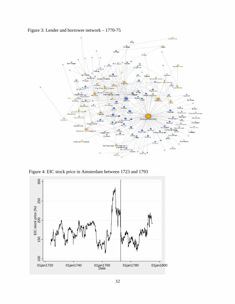
32

Figure 3: Lender and borrower network – 1770-75

Figure 4: EIC stock price in Amsterdam between 1723 and 1793

100

150

200

250

300

EIC

sto

ck p

rice

(%)

01jan1720 01jan1740 01jan1760 01jan1780 01jan1800Date

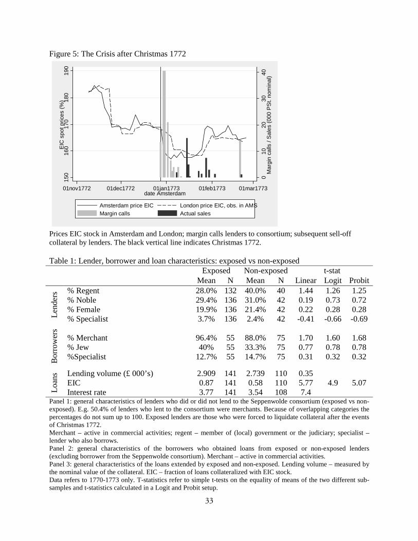
33

Figure 5: The Crisis after Christmas 1772

Prices EIC stock in Amsterdam and London; margin calls lenders to consortium; subsequent sell-off collateral by lenders. The black vertical line indicates Christmas 1772. Table 1: Lender, borrower and loan characteristics: exposed vs non-exposed Exposed Non-exposed t-stat Mean N Mean N Linear Logit Probit

Lend

ers % Regent 28.0% 132 40.0% 40 1.44 1.26 1.25

% Noble 29.4% 136 31.0% 42 0.19 0.73 0.72 % Female 19.9% 136 21.4% 42 0.22 0.28 0.28 % Specialist 3.7% 136 2.4% 42 -0.41 -0.66 -0.69

Bor

row

ers

% Merchant 96.4%

55

88.0%

75

1.70

1.60

1.68

% Jew %Specialist

40% 12.7%

55 55

33.3% 14.7%

75 75

0.77 0.31

0.78 0.32

0.78 0.32

Loan

s Lending volume (£ 000’s) 2.909 141 2.739 110 0.35 EIC Interest rate

0.87 3.77

141 141

0.58 3.54

110 108

5.77 7.4

4.9 5.07

Panel 1: general characteristics of lenders who did or did not lend to the Seppenwolde consortium (exposed vs non-exposed). E.g. 50.4% of lenders who lent to the consortium were merchants. Because of overlapping categories the percentages do not sum up to 100. Exposed lenders are those who were forced to liquidate collateral after the events of Christmas 1772. Merchant – active in commercial activities; regent – member of (local) government or the judiciary; specialist – lender who also borrows. Panel 2: general characteristics of the borrowers who obtained loans from exposed or non-exposed lenders (excluding borrower from the Seppenwolde consortium). Merchant – active in commercial activities. Panel 3: general characteristics of the loans extended by exposed and non-exposed. Lending volume – measured by the nominal value of the collateral. EIC – fraction of loans collateralized with EIC stock. Data refers to 1770-1773 only. T-statistics refer to simple t-tests on the equality of means of the two different sub-samples and t-statistics calculated in a Logit and Probit setup.

010

2030

40M

argi

n ca

lls /

Sal

es (0

00 P

St.

nom

inal

)

150

160

170

180

190

EIC

spo

t pric

es (%

)

01nov1772 01dec1772 01jan1773 01feb1773 01mar1773date Amsterdam

Amsterdam price EIC London price EIC, obs. in AMSMargin calls Actual sales

34

Table 2: Positions of the Seppenwolde syndicate, Christmas 1772 Member of the Syndicate Position (nominal)

EIC BoE

Hermanus van Seppenwolde £63,600 £49,500

Johannes van Seppenwolde £69,600 £17,000 Clifford & Chevalier £44,500 0 Pieter van Peene £2,000 £4,000 Total £179,700 £70,500 Total outstanding £3,194,080 £10,780,000 % syndicate in total outstanding 5.63% 0.65% Av. monthly turnover (1770-1772) £196,967 ? % syndicate in av. monthly turnover 91.23% ? Positions calculated at the end of 1772. Average monthly turnover is based on the turnover in the capital books of the respective companies. Actual market turnover would have been higher if transactions were netted out before mutations in the capital books were made. Table 3: Descriptive statistics, EIC stock returns over 6 month periods (overlapping)

Sample Prior to distress Distress period Full

1723-1772* 1770-73** 1723-1794 Mean 0.0051 -0.034 0.0028 Median 0.0068 -0.019 0.0053 σ 0.089 0.108 0.089 Skewness 0.248 -0.49 -0.07 Maximum loss -0.256 -0.358 -0.358 % of observations with loss>0.2

0.011 0.075 0.022

* first half ** first week of 1773 Table 4: Descriptive statistics - loan contracts

Variable Obs Mean Std. Dev. Min Max

Real value of collateral guilders) 418 36,271 27,734 4,782 238,058 Nominal (face) value of collateral (£)

420 1,910 1,608 300 15,000

Loan value (guilders) 422 28,969 23,244 2,200 210,000 Haircut 418 0.205 0.059 0.080 0.550 Interest rate (in %) 420 3.63 0.30 2.50 4.00 Non-EIC (BoE, SSC, 3% annuities)

405 0.102 0.042 -0.055 0.310

35

Table 5: Number of loans, lenders and borrowers, and collateral before/after Christmas 1772 Panel (A): Number of loan contracts by period From exposed Loans consortium yes No yes no Before Xmas 1772 217 145 232 130 After Xmas 1772 41 15 . 56

Panel (B): Number of lenders and borrowers by period # of lenders; exposed # of borrowers; from exposed yes no yes no Before Xmas 1772 77 68 32 36 After Xmas 1772 17 9 20 11 # new lenders/borrowers after Xmas 1772

. 1 12 4

% loans accounted for by new lenders/borrowers

. 11% 44% 40%

Panel (C): Types of collateral used by period EIC BoE Other Lenders exposed Lenders exposed Lenders exposed yes no Yes no yes no Before Xmas 1772 84% 55% 14% 38% 2% 7% After Xmas 1772 83% 88% 0% 6% 17% 6% The table presents descriptive statistics before and after Christmas 1772. Panel (A) presents the number of new loans that were extended, differentiated by whether loans were extended by lenders who were exposed to the consortium around Christmas 1772 or by whether loans were taken up by the Seppenwolde consortium. Exposed lenders are those who were forced to liquidate collateral after the default. Some loans taken up by the consortium were repaid before Christmas 1772. This explains why the total number of consortium loans is larger than the number of loans extended by exposed lenders. Panel (B) lists the number of lenders and borrowers. Lenders are differentiated by whether they were exposed or not. Borrowers are differentiated by whether they borrowed from exposed lenders yes or no. The panel also lists the number of new lenders and borrowers that entered the market after Christmas 1772. New borrowers are differentiated by whether they borrow from exposed or non-exposed lenders. We also calculate the percentage of total lending extended by new lenders / taken up by new borrowers. Total lending is measured in nominal or face value of the collateral. Panel (C) presents the type of collateral that was used in the loan transactions, again differentiated by whether lenders were exposed yes or no. EIC is East India Company, BoE is Bank of England, Other includes South Sea Company and a number of government securities. Table 6: Simple difference-in-difference estimate – EIC stock only Before Christmas 1772 After Christmas 1772 ∆ Not exposed 0.211 0.193 -0.018 Exposed 0.207 0.261 0.054***

-0.004 0.069*** 0.072*** Average haircuts on EIC stock, differentiated by exposed and non-exposed lenders, before and after Christmas 1772. Haircuts are calculated as the fraction of the collateral value that is not financed with a loan. Exposed lenders are those who were forced to liquidate collateral after the events of Christmas 1772. Observations refer to new contracts. Averages are weighed by the nominal (face) value of the collateral. The simple diff-in-diff estimate is in bold in the lower right corner. *** indicates significance at the 1% level.

36

Table 7: Haircut change – benchmark estimates

(1)

Pooled OLS

(2) Pooled OLS

(3) FE

(4) FE

(5) FE

Exposed -0.005 -0.003 0.017 -0.000 0.028 (0.005) (0.005) (0.014) (0.006) (0.013)** Exposed * Post 1772 0.076 0.066 0.061 0.040 0.063 (0.022)*** (0.023)*** (0.036)* (0.024)* (0.036)* non-EIC -0.059 -0.056 -0.049 -0.052 -0.047 (0.006)*** (0.006)*** (0.011)*** (0.008)*** (0.014)*** Lender merchant 0.007 0.004 (0.007) (0.007) Lender regent -0.005 -0.004 (0.006) (0.006) Lender noble 0.003 0.004 (0.005) (0.006) Lender female -0.007 -0.003 (0.007) (0.007) Lender specialist -0.012 -0.007 (0.007)* (0.009) Borrower merchant -0.039 -0.042 (0.016)** (0.022)* Borrower specialist -0.004 -0.018 (0.011) (0.017) Borrower Jewish 0.050 0.047 (0.011)*** (0.015)*** Constant 0.219 0.245 0.235 0.211 0.174 (0.006)*** (0.017)*** (0.026)*** (0.012)*** (0.036)*** Year dummies Y Y Y Y Y Lender FE N N Y N Y Borrower FE N N N Y Y N 418 387 418 387 418 N (if balanced) 166 77 33 # lenders 177 152 177 152 177 # borrowers 72 70 72 70 72 R2 0.334 0.440 0.632 0.659 0.802 Regression estimates for all English securities. Observations refer to new contracts and are weighted by the nominal (face) value of the collateral. Haircuts are calculated as the fraction of the collateral value that is not financed with a loan. Exposed lenders are those who were forced to liquidate collateral after the events of Christmas 1772. The interaction between the exposed and the post-1772 dummies captures the diff-in-diff effect. Lender and borrower fixed effects refer to fixed effects on the family/firm level. Robust standard errors (clustered at the lender level) are reported in parentheses. * p < 0.10, ** p < 0.05, *** p < 0.01

37

Table 8: Haircuts and lender characteristics (1) (2) (3) (4) (5) (6) Exposed -0.002 -0.003 -0.003 -0.003 -0.003 -0.003 (0.005) (0.005) (0.004) (0.005) (0.005) (0.005) Exposed * Post 1772 0.062 0.068 0.062 0.064 0.065 0.061 (0.021)*** (0.023)*** (0.023)*** (0.022)*** (0.023)*** (0.021)*** non-EIC -0.055 -0.056 -0.056 -0.056 -0.056 -0.056 (0.006)*** (0.006)*** (0.006)*** (0.006)*** (0.006)*** (0.006)*** Merchant * Post 1772 0.033 0.022 (0.019)* (0.063) Regent * Post 1772 -0.015 0.008 (0.017) (0.056) Noble * Post 1772 -0.040 -0.029 (0.019)** (0.023) Female * Post 1772 -0.026 -0.002 (0.029) (0.053) Specialist* Post1772 0.005 -0.005 (0.047) (0.041) Constant 0.241 0.243 0.239 0.244 0.245 0.239 (0.018)*** (0.017)*** (0.017)*** (0.017)*** (0.017)*** (0.018)*** Year dummies Y Y Y Y Y Y Lender & borrower observables

Y Y Y Y Y Y

N 387 387 387 387 387 387 R2 0.448 0.442 0.452 0.443 0.440 0.453 # lenders 152 152 152 152 152 152 Pooled OLS estimates for all English securities. Observations refer to new contracts and are weighted by the nominal (face) value of the collateral. Haircuts are calculated as the fraction of the collateral value that is not financed with a loan. Exposed lenders are those who were forced to liquidate collateral after the events of Christmas 1772. The interaction between the exposed and the post-1772 dummies captures the diff-in-diff effect. Lender and borrower observables are as in Table 6. Merchant – active in commerce; regent – member of (local) government or judiciary; specialist – lenders also active as borrower. Robust standard errors (clustered at the lender level) are reported in parentheses. * p < 0.10, ** p < 0.05, *** p < 0.01

38

Table 9: Haircuts and borrower characteristics (1) (2) (3) (4) (5) Exposed -0.003 -0.003 -0.004 -0.003 -0.001 (0.005) (0.005) (0.005) (0.004) (0.006) Exposed * Post 1772 0.067 0.066 0.076 0.077 0.056 (0.023)*** (0.024)*** (0.023)*** (0.025)*** (0.024)** non-EIC -0.056 -0.056 -0.056 -0.057 -0.051 (0.006)*** (0.006)*** (0.006)*** (0.006)*** (0.008)*** Merchant * Post 1772 0.002 0.038 (0.048) (0.050) Specialist * Post 1772 -0.038 -0.032 (0.024) (0.022) Jewish * Post 1772 -0.056 -0.056 (0.025)** (0.025)** Constant 0.245 0.241 0.236 0.242 0.207 (0.016)*** (0.018)*** (0.019)*** (0.015)*** (0.012)*** Year dummies Y Y Y Y Y Lender & borrower observables

Y Y Y Y

Borrower-time FE N N N N Y N 387 387 387 387 387 R2 0.440 0.447 0.458 0.464 0.691 # groups (borrowers) 70 70 70 70 70 Table 10: Probability of lender matched to a repeat borrower (1) (2) (3) (4) (5) (6) OLS OLS Logit Logit Probit Probit Post 1772 -0.211 -0.196 -0.211 -0.209 -0.211 -0.207 (0.050)*** (0.108)* (0.050)*** (0.110)* (0.050)*** (0.104)** Exposed 0.026 0.020 0.021 (0.109) (0.086) (0.091) Exposed * Post -0.018 -0.002 -0.006 1772 (0.122) (0.196) (0.173) N 224 224 224 224 224 224 R2 0.050 0.050 Dependent variable: is a lender matched to a repeat borrower (one (s)he has been matched to before) 0: no; 1: yes. Unit of observation: new loan contracts. To minimize measurement error of the repeat borrower variable, transactions after Jan 1, 1772 only. Post 1772 is a dummy for contracts signed after Christmas 1772. Exposed is a dummy for lenders who were exposed to the Seppenwolde bankruptcy. We report marginal effects. Estimates should be interpreted as the change in the probability of being matched with a repeat borrower in response to a change in the dummy variables from 0 to 1. Robust standard errors (clustered at the lender level) in parentheses. * p < 0.10, ** p < 0.05, *** p < 0.01

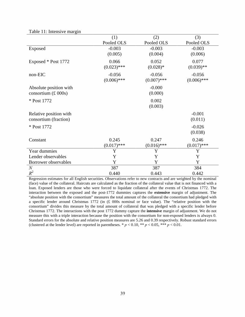
39

Table 11: Intensive margin (1) (2) (3) Pooled OLS Pooled OLS Pooled OLS Exposed -0.003 -0.003 -0.003 (0.005) (0.004) (0.006) Exposed * Post 1772 0.066 0.052 0.077 (0.023)*** (0.028)* (0.039)** non-EIC -0.056 -0.056 -0.056 (0.006)*** (0.007)*** (0.006)*** Absolute position with consortium (£ 000s)

-0.000 (0.000)

* Post 1772 0.002 (0.003) Relative position with consortium (fraction)

-0.001 (0.011)

* Post 1772 -0.026 (0.038) Constant 0.245 0.247 0.246 (0.017)*** (0.016)*** (0.017)*** Year dummies Y Y Y Lender observables Y Y Y Borrower observables Y Y Y N 387 387 384 R2 0.440 0.443 0.442 Regression estimates for all English securities. Observations refer to new contracts and are weighted by the nominal (face) value of the collateral. Haircuts are calculated as the fraction of the collateral value that is not financed with a loan. Exposed lenders are those who were forced to liquidate collateral after the events of Christmas 1772. The interaction between the exposed and the post-1772 dummies captures the extensive margin of adjustment. The “absolute position with the consortium” measures the total amount of the collateral the consortium had pledged with a specific lender around Christmas 1772 (in (£ 000s nominal or face value). The “relative position with the consortium” divides this measure by the total amount of collateral that was pledged with a specific lender before Christmas 1772. The interactions with the post 1772 dummy capture the intensive margin of adjustment. We do not measure this with a triple interaction because the position with the consortium for non-exposed lenders is always 0. Standard errors for the absolute and relative position measures are 5.26 and 0.39 respectively. Robust standard errors (clustered at the lender level) are reported in parentheses. * p < 0.10, ** p < 0.05, *** p < 0.01.

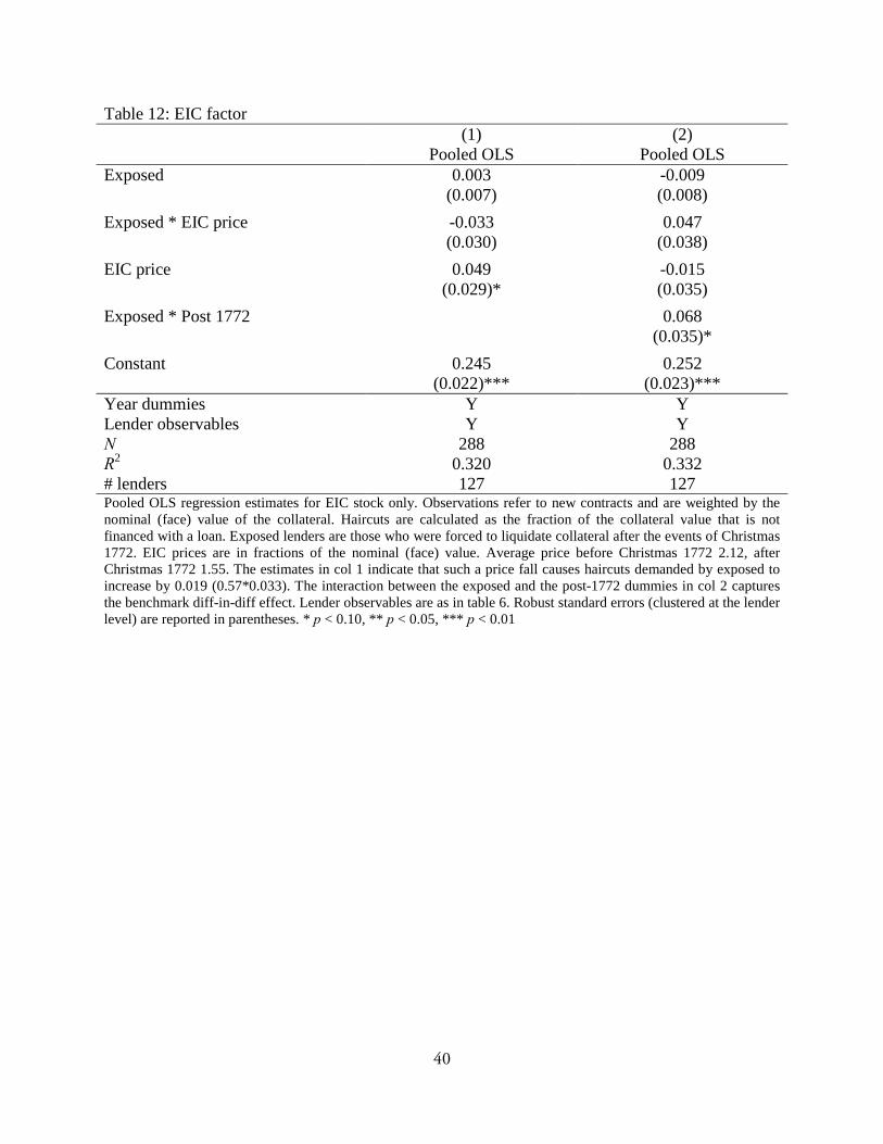
40

Table 12: EIC factor (1) (2) Pooled OLS Pooled OLS Exposed 0.003 -0.009 (0.007) (0.008) Exposed * EIC price -0.033 0.047 (0.030) (0.038) EIC price 0.049 -0.015 (0.029)* (0.035) Exposed * Post 1772 0.068 (0.035)* Constant 0.245 0.252 (0.022)*** (0.023)*** Year dummies Y Y Lender observables Y Y N 288 288 R2 0.320 0.332 # lenders 127 127 Pooled OLS regression estimates for EIC stock only. Observations refer to new contracts and are weighted by the nominal (face) value of the collateral. Haircuts are calculated as the fraction of the collateral value that is not financed with a loan. Exposed lenders are those who were forced to liquidate collateral after the events of Christmas 1772. EIC prices are in fractions of the nominal (face) value. Average price before Christmas 1772 2.12, after Christmas 1772 1.55. The estimates in col 1 indicate that such a price fall causes haircuts demanded by exposed to increase by 0.019 (0.57*0.033). The interaction between the exposed and the post-1772 dummies in col 2 captures the benchmark diff-in-diff effect. Lender observables are as in table 6. Robust standard errors (clustered at the lender level) are reported in parentheses. * p < 0.10, ** p < 0.05, *** p < 0.01

41

FOR ONLINE PUBLICATION Appendix A: Sample contract – original and English translation (SAA 10,602, F. 1309) Heden den 2e November 1772 compareerde voor mij Daniel van den Brink Openbaar Notaris binnen Amsterdam de heer Raphael de Abraham Mendes da Costa, voor en in de naam van zijn Compagnie luidende Abraham de Raphael Mendes da Costa & Co, Kooplieden binnen deeze stadt

Today, November 2, 1772 appeared before me, Daniel van den Brink, Public Notary in the City of Amsterdam, mr. Raphael de Abraham Mendes da Costa, for and in the name of his company called Abraham de Raphael Mendes da Costa & Co, merchants in this town (hereafter: “the party present”).

en bekende bij deeze wel en deugdelijk schuldig te wezen aan de Heer Ananias Willink, meede Coopman alhier de somma van 24.000 guldens bankgeld spruytende uyt hoofden en ter saake van sodanige somma als de selve den 22e Oktober laatstleden aan syn comp[arants] voorn[oemde] Compagnie heeft afgeschreven, […] en welke somma van f. 24.000 Bankgeld hij Comparant in de naam van zijn voorn[oemde] compagnie aanneemt

And declared to be indebted to mr. Ananias Willink, also merchant in this city for the sum of 24,000 guilders banco, originating from and relating to a withdrawal of such sum on October 22 last in favor of the present party’s said company, and the present party accepting that sum of 24,000 guilders banco in the name of said company.

en belooft aan voorn[oemde] Heer Ananias Willink of zijn Co[mpagnies] rechthebbende kosten schadeloos alhier weeder te zullen restitueren en voldoen binnen de tijdt van ses maanden te reekenen van den 6 Oktober deeses jaars met den Interest van dien tegens vier percent ’t jaar en bij prolongatie gelijke interest

And promises to said mr Ananias Willink, or his company’s legal representative, to return this sum (including any costs incurred), within the time of six months, counting from October 6 this year, with the interest of 4% annual, and in case of prolongation the same interest.

en zulks tot de volle en effectueele betaalinge toe tog de interessen te betaalen ieder 6 maanden des zo zal bij opeischinge of aflossinge den een den ander ses weeken voor de vervaltijd waarschouwent

And [promises] to pay the full and effective payment of the interest every six months In case that the contract is not prolonged he will be notified 6 weeks in advance.

tot nakominge deezes verbind hij comparant zijn en zijn gemelde Compagnons persoon en goederen als na rechten en specialijk sodanige vijftienhonderd ponden sterling capitaal actien in de d’Oost Indische Compagnie van Engeland als tot London voor reekening van zijn comparants

To honor this agreement, the present party pledges his own body and goods and especially 1500 Pounds Sterling capital in the stocks of the English East India Company, which have been transferred in London from the account of the present party’s company to the account of said mr.

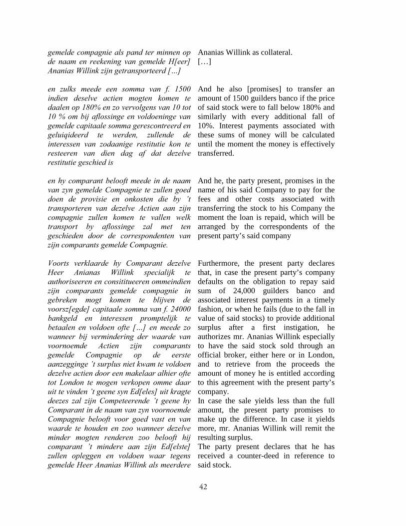
42

gemelde compagnie als pand ter minnen op de naam en reekening van gemelde H[eer] Ananias Willink zijn getransporteerd […]

Ananias Willink as collateral. […]

en zulks meede een somma van f. 1500 indien deselve actien mogten komen te daalen op 180% en zo vervolgens van 10 tot 10 % om bij aflossinge en voldoeninge van gemelde capitaale somma gerescontreerd en geluiqideerd te werden, zullende de interessen van zodaanige restitutie kon te resteeren van dien dag af dat dezelve restitutie geschied is

And he also [promises] to transfer an amount of 1500 guilders banco if the price of said stock were to fall below 180% and similarly with every additional fall of 10%. Interest payments associated with these sums of money will be calculated until the moment the money is effectively transferred.

en hy comparant belooft meede in de naam van zyn gemelde Compagnie te zullen goed doen de provisie en onkosten die by ’t transporteren van dezelve Actien aan zijn compagnie zullen komen te vallen welk transport by aflossinge zal met ten geschieden door de correspondenten van zijn comparants gemelde Compagnie.

And he, the party present, promises in the name of his said Company to pay for the fees and other costs associated with transferring the stock to his Company the moment the loan is repaid, which will be arranged by the correspondents of the present party’s said company

Voorts verklaarde hy Comparant dezelve Heer Anianas Willink specialijk te authoriseeren en consititueeren ommeindien zijn comparants gemelde compagnie in gebreken mogt komen te blijven de voorsz[egde] capitaale somma van f. 24000 bankgeld en interessen promptelijk te betaalen en voldoen ofte […] en meede zo wanneer bij vermindering der waarde van voornoemde Actien zijn comparants gemelde Compagnie op de eerste aanzegginge ’t surplus niet kwam te voldoen dezelve actien door een makelaar alhier ofte tot London te mogen verkopen omme daar uit te vinden ’t geene syn Ed[eles] uit kragte deezes zal zijn Competeerende ’t geene hy Comparant in de naam van zyn voornoemde Compagnie belooft voor goed vast en van waarde te houden en zoo wanneer dezelve minder mogten renderen zoo belooft hij comparant ’t mindere aan zijn Ed[elste] zullen opleggen en voldoen waar tegens gemelde Heer Ananias Willink als meerdere

Furthermore, the present party declares that, in case the present party’s company defaults on the obligation to repay said sum of 24,000 guilders banco and associated interest payments in a timely fashion, or when he fails (due to the fall in value of said stocks) to provide additional surplus after a first instigation, he authorizes mr. Ananias Willink especially to have the said stock sold through an official broker, either here or in London, and to retrieve from the proceeds the amount of money he is entitled according to this agreement with the present party’s company. In case the sale yields less than the full amount, the present party promises to make up the difference. In case it yields more, mr. Ananias Willink will remit the resulting surplus. The party present declares that he has received a counter-deed in reference to said stock.

43

aan zijn comparants gemelde Compagnie zal goed doen en hij Comparant bekende van syn Ed[ele] wegens voorsz[egde] actien een renvers[aal] te hebben ontvangen

Actum Amsterdam, 2 November 1772 Signed in Amsterdam, November 2, 1772

44

Appendix B: Interest rates, total lending and concentration of lending Interest rates The model predicts that interest rates should not change differentially after the Seppenwolde

default. By giving all bargaining power to the borrower, interest rates will always equal the risk

free rate, independent of the type of match. In this subsection we do two things. First, we argue

that a richer model that allocates some bargaining power to the lenders has similar predictions.

Second, we show that the empirical findings are consistent with the market balancing through

haircuts rather than interest rates.

What pins down interest rates in the model developed in section II when we allocate

(some) bargaining power to the lender? Do interest rates on loans of types 1 and 2 change

differentially? The interest rate predictions that follow from such an extended model are

ambiguous. After being matched, agents bargain over the match-specific surplus. This is defined

as and measures the gains to a type 3 agent from accepting a loan of type

relative to waiting for another match in the future. Suppose that agents engage in Nash

bargaining and always get a fixed fraction of the surplus. Transfers between borrowers and

lenders take place through interest payments. The interest rate therefore equals the risk free rate

(which is normalized to zero) plus the transfer from borrower to lender divided by the size of the

loan. Consider the case where the beliefs of type 1 and 2 agents are initially similar and focus on

the impact of a drop in . In that case, type 1 lenders become less attractive and the match

specific surplus will be lower than for a type 2 lender, i.e. . Type 1 and 2

lenders will always get the same fraction of the match-specific surplus, but the absolute value of

their share is smaller for type 1 agents. This would suggest that type 1 borrowers charge lower

interest rates. However, the size of the loan they extend is also smaller. Both numerator and

denominator decrease. The net effect is small and the sign is ambiguous (it depends on the exact

parameter values).

We next explore the empirical evidence. Figure B. 1 shows the development of interest

rates over time. The figure shows that the interest rates that are charged by exposed and non-

exposed lenders track each other very closely, both before and after Christmas 1772. This is

confirmed by figure Figure B. 2 that presents the distributions of interest rates that are charged

by exposed and non-exposed. The figure shows a shift to lower interest rates after Christmas

1772 that occurs for both groups of lenders.

45

We test this econometrically in Table B. 1. The table confirms that there is no differential

change in the interest rate (see discussion in the main text). The table further shows that non-EIC

securities attracted lower interest rates, but the difference is small – between 8 and 10 basis

points. In a number of specifications we also find that lenders exposed to the syndicate initially

charged somewhat higher interest rates both before and after the event. In col (1), the effect is

statistically significant but economically small – the estimated coefficient implies a difference of

8 basis points. When we control for lender and borrower type dummies the coefficient falls to

about 5 basis points and becomes statistically insignificant.

Total lending

Did lending volume per lender change as a result of the Seppenwolde episode? Table B. 3

examines total lending volume per lender. We analyze both total lending (cols 1 – 3) and lending

excluding loans made to the Seppenwolde consortium (all before Christmas 1772) (cols 4 – 6).

Those who were exposed lent more than the rest before the crisis, on average. Lending against

assets other than the EIC was also associated with higher lending volume.

Most importantly, the statistical results suggest that those affected by the Seppenwolde

crisis differentially reduced their lending thereafter. Especially in the fixed effect estimate of col

3, this increase seems to have been by a quantitatively considerable margin. When we exclude

loans made to the Seppenwolde consortium, the treatment effect is reduced but is still negative.

Depending on the specification, exposed lenders lent 30 to 50% less after Christmas 1773. Even

though these effects are economically important, none of them is actually statistically significant.

Concentration of lending

To test if random matching of lenders and borrowers can explain the nature of lending in our

sample, we calculate the Herfindahl index for every lender during the pre-crisis period:

where is the share of lending by lender � to an individual borrower �. If lenders repeatedly

lent to the same borrower, to the exclusion of other investors, we would expect a high Herfindahl

index. The left panel of Figure B. 3 presents the actual distribution of these Herfindahl indices

for all lenders in ours sample. Many lenders only entered into a single transaction; these are

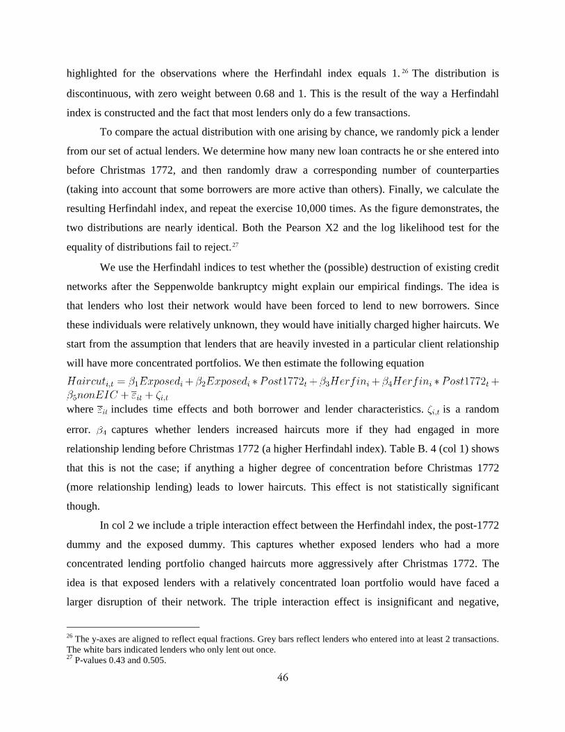
46

highlighted for the observations where the Herfindahl index equals 1. 26 The distribution is

discontinuous, with zero weight between 0.68 and 1. This is the result of the way a Herfindahl

index is constructed and the fact that most lenders only do a few transactions.

To compare the actual distribution with one arising by chance, we randomly pick a lender

from our set of actual lenders. We determine how many new loan contracts he or she entered into

before Christmas 1772, and then randomly draw a corresponding number of counterparties

(taking into account that some borrowers are more active than others). Finally, we calculate the

resulting Herfindahl index, and repeat the exercise 10,000 times. As the figure demonstrates, the

two distributions are nearly identical. Both the Pearson X2 and the log likelihood test for the

equality of distributions fail to reject.27

We use the Herfindahl indices to test whether the (possible) destruction of existing credit

networks after the Seppenwolde bankruptcy might explain our empirical findings. The idea is

that lenders who lost their network would have been forced to lend to new borrowers. Since

these individuals were relatively unknown, they would have initially charged higher haircuts. We

start from the assumption that lenders that are heavily invested in a particular client relationship

will have more concentrated portfolios. We then estimate the following equation

where includes time effects and both borrower and lender characteristics. is a random

error. captures whether lenders increased haircuts more if they had engaged in more

relationship lending before Christmas 1772 (a higher Herfindahl index). Table B. 4 (col 1) shows

that this is not the case; if anything a higher degree of concentration before Christmas 1772

(more relationship lending) leads to lower haircuts. This effect is not statistically significant

though.

In col 2 we include a triple interaction effect between the Herfindahl index, the post-1772

dummy and the exposed dummy. This captures whether exposed lenders who had a more

concentrated lending portfolio changed haircuts more aggressively after Christmas 1772. The

idea is that exposed lenders with a relatively concentrated loan portfolio would have faced a

larger disruption of their network. The triple interaction effect is insignificant and negative,

26 The y-axes are aligned to reflect equal fractions. Grey bars reflect lenders who entered into at least 2 transactions. The white bars indicated lenders who only lent out once. 27 P-values 0.43 and 0.505.

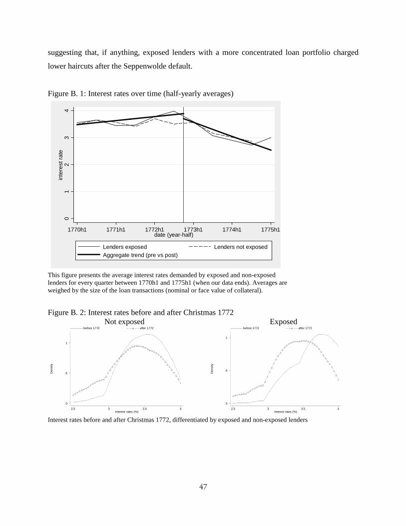
47

suggesting that, if anything, exposed lenders with a more concentrated loan portfolio charged

lower haircuts after the Seppenwolde default.

Figure B. 1: Interest rates over time (half-yearly averages)

This figure presents the average interest rates demanded by exposed and non-exposed lenders for every quarter between 1770h1 and 1775h1 (when our data ends). Averages are weighed by the size of the loan transactions (nominal or face value of collateral).

Figure B. 2: Interest rates before and after Christmas 1772 Not exposed Exposed

Interest rates before and after Christmas 1772, differentiated by exposed and non-exposed lenders

01

23

4in

tere

st ra

te

1770h1 1771h1 1772h1 1773h1 1774h1 1775h1date (year-half)

Lenders exposed Lenders not exposedAggregate trend (pre vs post)

Den

sity

Interest rates (%)

before 1772 after 1772

2.5 3 3.5 4

0

.5

1

Den

sity

Interest rates (%)

before 1772 after 1772

2.5 3 3.5 4

0

.5

1

48

Figure B. 3: Herfindahl indices – actual vs simulated

For each lender we calculate the Herfindahl index of its lending before Christmas 1772. In addition, we construct a random distribution of Herfindahl indices. We randomly pick a lender from our set of lenders; we determine how many (x) new loan contracts it entered into before Christmas 1772; we randomly draw x counterparties (taking into account that some borrowers are more active than others); and we calculate the resulting Herfindahl index. We do this 10,000 times. The y-axes are aligned to reflect equal fractions. Grey bars reflect lenders who entered into at least 2 transactions. The white bars indicated lenders who only lent out once.

Tests on the equality of the distributions: Test statistic pvalue Pearson's X2 83.8 0.435 Log likelihood ratio 37.9 0.505 Obs. (Unique values) 178 (84)

050

100

150

Freq

uenc

y

0 .2 .4 .6 .8 1Herfindahl

Actual Herfindahl indices

020

0040

0060

0080

00Fr

eque

ncy

0 .2 .4 .6 .8 1Herfindahl

Herfindahl indices from random draws

Lenders with single transaction Lenders with multiple transactions

49

Table B. 1: Interest rates – benchmark estimates

(1)

Pooled OLS (2)

Pooled OLS (3) FE

(4) FE

(5) FE

Exposed 0.072 0.048 -0.116 0.074 -0.152 (0.036)** (0.034) (0.048)** (0.041)* (0.057)*** Exposed * Post 1772 -0.049 -0.034 -0.077 0.035 0.073 (0.099) (0.099) (0.130) (0.113) (0.219) non-EIC -0.078 -0.093 -0.084 -0.104 -0.078 (0.036)** (0.034)*** (0.050)* (0.049)** (0.053) Lender merchant 0.126 0.090 (0.057)** (0.063) Lender regent -0.016 -0.017 (0.044) (0.050) Lender noble 0.024 0.027 (0.045) (0.047) Lender female 0.027 0.001 (0.049) (0.043) Lender specialist -0.023 -0.024 (0.032) (0.041) Borrower merchant -0.141 -0.060 (0.084)* (0.088) Borrower specialist -0.080 -0.096 (0.043)* (0.066) Borrower Jewish 0.018 -0.016 (0.035) (0.046) Constant 3.527 3.637 3.739 3.559 3.879 (0.036)*** (0.096)*** (0.102)*** (0.071)*** (0.177)*** Year dummies Y Y Y Y Y Lender FE N N Y N Y Borrower FE N N N Y Y N 418 386 418 386 418 N (if balanced panel) 166 77 33 # lenders 177 152 177 152 177 # borrowers 72 70 72 70 72 R2 0.511 0.564 0.744 0.699 0.836 Regression estimates for all English securities. Observations refer to new contracts and are weighted by the nominal (face) value of the collateral. Exposed lenders are those who were forced to liquidate collateral after the events of Christmas 1772. The interaction between the exposed and the post-1772 dummies captures the diff-in-diff effect. Lender and borrower fixed effects refer to fixed effects on the family/firm level. Robust standard errors (clustered at the lender level) are reported in parentheses. * p < 0.10, ** p < 0.05, *** p < 0.01

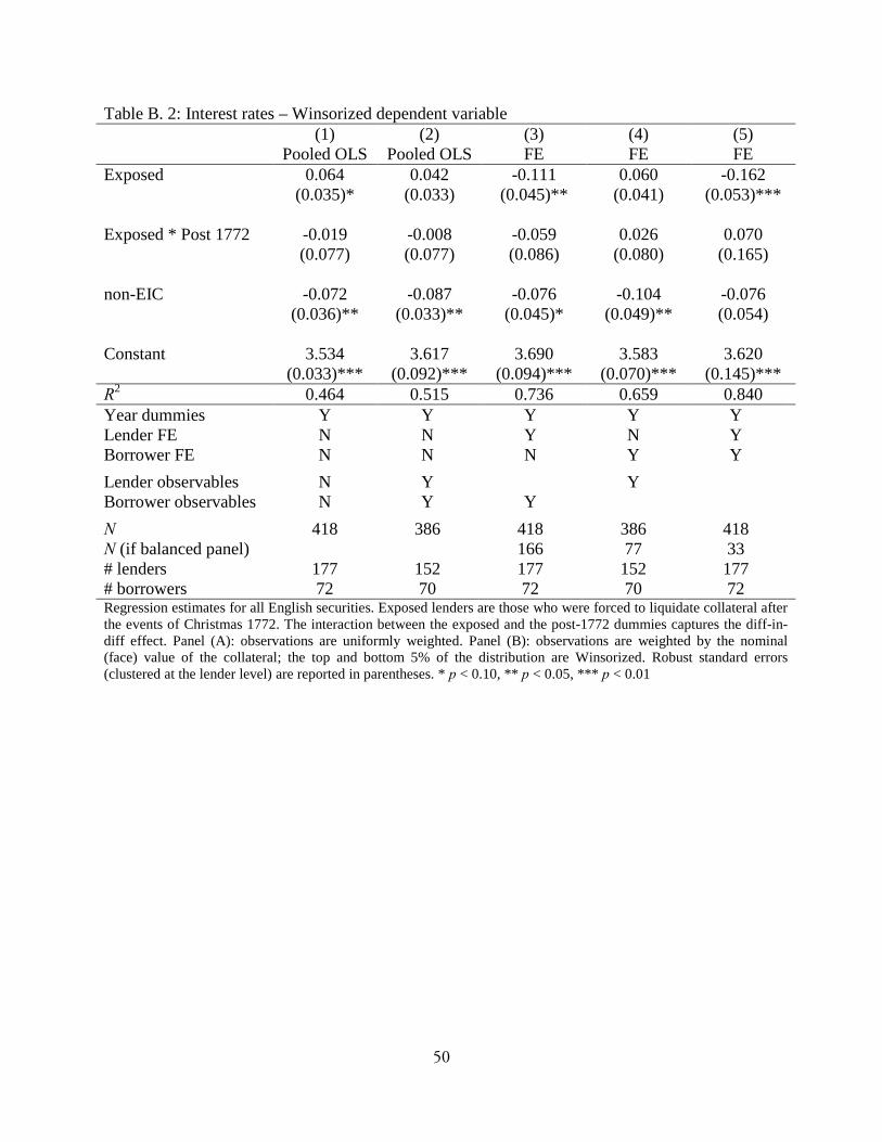
50

Table B. 2: Interest rates – Winsorized dependent variable (1) (2) (3) (4) (5) Pooled OLS Pooled OLS FE FE FE Exposed 0.064 0.042 -0.111 0.060 -0.162 (0.035)* (0.033) (0.045)** (0.041) (0.053)*** Exposed * Post 1772 -0.019 -0.008 -0.059 0.026 0.070 (0.077) (0.077) (0.086) (0.080) (0.165) non-EIC -0.072 -0.087 -0.076 -0.104 -0.076 (0.036)** (0.033)** (0.045)* (0.049)** (0.054) Constant 3.534 3.617 3.690 3.583 3.620 (0.033)*** (0.092)*** (0.094)*** (0.070)*** (0.145)*** R2 0.464 0.515 0.736 0.659 0.840 Year dummies Y Y Y Y Y Lender FE N N Y N Y Borrower FE N N N Y Y Lender observables N Y Y Borrower observables N Y Y N 418 386 418 386 418 N (if balanced panel) 166 77 33 # lenders 177 152 177 152 177 # borrowers 72 70 72 70 72 Regression estimates for all English securities. Exposed lenders are those who were forced to liquidate collateral after the events of Christmas 1772. The interaction between the exposed and the post-1772 dummies captures the diff-in-diff effect. Panel (A): observations are uniformly weighted. Panel (B): observations are weighted by the nominal (face) value of the collateral; the top and bottom 5% of the distribution are Winsorized. Robust standard errors (clustered at the lender level) are reported in parentheses. * p < 0.10, ** p < 0.05, *** p < 0.01

51

Table B. 3: Total lending Including Van Seppenwolde Excluding Van Seppenwolde (1) (2) (3) (4) (5) (6) Pooled

OLS Pooled OLS

FE Pooled OLS

Pooled OLS

FE

Exposed 1.911 2.144 2.489 1.433 1.783 0.188 (0.935)** (1.166)* (2.054) (0.923) (1.212) (2.375) Post 1772 0.326 0.175 -0.104 0.742 0.764 0.129 (0.487) (0.610) (1.713) (0.402)* (0.517) (2.275) Exposed * Post 1772

-1.186 -1.465 -3.648 -0.749 -1.232 -1.640

(0.913) (1.163) (3.341) (0.988) (1.081) (2.447) non-EIC 3.337 3.499 2.782 2.243 1.832 1.720 (1.346)** (1.700)** (3.612) (0.895)** (0.954)* (3.345) Constant 2.190 3.050 2.287 1.884 4.147 2.864 (0.462)*** (1.405)** (1.492) (0.335)*** (1.518)*** (1.272)** Year dummies Y Y Y Y Y Y Lender observables

N Y N Y

Lender FE N N Y N N Y N 202 175 202 128 113 128 N (if balanced panel)

50 30

R2 0.040 0.080 0.880 0.050 0.150 0.955 # lenders 177 152 177 113 99 113 Regression estimates for total lending at the lender level on the collateral of all English securities. Total lending is calculated before and after Christmas 1772; in £000s of nominal (face) value. Exposed lenders are those who were forced to liquidate collateral after the events of Christmas 1772. The interaction between the post-1772 and the exposed dummies captures the diff-in-diff effect. Lender observables are as in Table 6. Lender fixed effects refer to fixed effects on the family level. Robust standard errors (clustered at the lender level) are reported in parentheses. * p < 0.10, ** p < 0.05, *** p < 0.01.

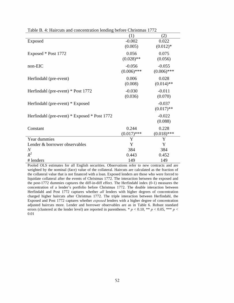
52

Table B. 4: Haircuts and concentration lending before Christmas 1772 (1) (2) Exposed -0.002 0.022 (0.005) (0.012)* Exposed * Post 1772 0.056 0.075 (0.028)** (0.056) non-EIC -0.056 -0.055 (0.006)*** (0.006)*** Herfindahl (pre-event) 0.006 0.028 (0.008) (0.014)** Herfindahl (pre-event) * Post 1772 -0.030 -0.011 (0.036) (0.070) Herfindahl (pre-event) * Exposed -0.037 (0.017)** Herfindahl (pre-event) * Exposed * Post 1772 -0.022 (0.088) Constant 0.244 0.228 (0.017)*** (0.018)*** Year dummies Y Y Lender & borrower observables Y Y N 384 384 R2 0.443 0.452 # lenders 149 149 Pooled OLS estimates for all English securities. Observations refer to new contracts and are weighted by the nominal (face) value of the collateral. Haircuts are calculated as the fraction of the collateral value that is not financed with a loan. Exposed lenders are those who were forced to liquidate collateral after the events of Christmas 1772. The interaction between the exposed and the post-1772 dummies captures the diff-in-diff effect. The Herfindahl index (0-1) measures the concentration of a lender’s portfolio before Christmas 1772. The double interaction between Herfindahl and Post 1772 captures whether all lenders with higher degrees of concentration charged higher haircuts after Christmas 1772. The triple interaction between Herfindahl, the Exposed and Post 1772 captures whether exposed lenders with a higher degree of concentration adjusted haircuts more. Lender and borrower observables are as in Table 6. Robust standard errors (clustered at the lender level) are reported in parentheses. * p < 0.10, ** p < 0.05, *** p < 0.01

53

Appendix C: Additional figures and tables Figure C. 1: Kernel densities haircuts before Christmas 1772

Raw vs corrected for year dummies and borrower fixed effects

Figure C. 2: Surplus on loans to consortium

Distributions of the ‘surplus’ on secured loans (the difference between the value of the collateral and the loan), right after the issuing of margin calls on December 29th and after the actual execution of the underlying collateral.

Den

sity

Haircuts

Raw Corrected for year and borr. FE

.1 .2 .3 .4 .5

0

2

4

05

1015

dens

ity

0 .05 .1 .15 .2surplus (fraction of collateral value)

Margin Call (paper) Execution (realized)

54

Figure C. 3: Distribution of EIC returns

Returns calculated over 6 month periods (overlapping). Vertical line indicates the 6 month return over the second half of 1772. Figure C. 4: Haircuts before and after Christmas 1772

Not exposed Exposed

Haircuts before and after Christmas 1772, differentiated by exposed and non-exposed lenders

Den

sity

6 month returns (%)

1723 - 1772 (first half) 1770 - 1773 (first week)

-30 -20 -10 0 10 20 30

0

.02

.04

Den

sity

Haircuts

before 1772 after 1772

.1 .2 .3 .4 .5

0

2

4

Den

sity

Haircuts

before 1772 after 1772

.1 .2 .3 .4 .5

0

2

4

55

Table C. 1: Haircuts and time since event

(1) (2) (3) (4) (5)

Pooled OLS

Pooled OLS

FE FE FE

Exposed -0.005 -0.003 -0.000 (0.005) (0.005) (0.006) Exposed * Post 1772 0.097 0.086 0.086 0.054 0.101 (0.030)*** (0.033)*** (0.046)* (0.030)* (0.045)** Time since event -0.001 0.023 0.008 -0.065 0.010 (0.058) (0.059) (0.066) (0.058) (0.073) Exposed * time since event

-0.051 -0.041 -0.051 -0.031 -0.058

(0.044) (0.044) (0.045) (0.042) (0.048) non-EIC -0.058 -0.055 -0.047 -0.053 -0.046 (0.006)*** (0.007)*** (0.012)*** (0.008)*** (0.014)*** Constant 0.218 0.244 0.243 0.212 0.460 (0.007)*** (0.018)*** (0.026)*** (0.012)*** (0.032)*** Year dummies Y Y Y Y Y Lender FE N N Y N Y Borrower FE N N N Y Y Lender observables N Y Y Borrower observables N Y Y N 418 387 418 387 418 N (if balanced panel) 166 77 33 R2 0.334 0.440 0.632 0.659 0.802 # groups (lenders) 177 152 177 152 177 # groups (borrowers) 72 70 72 70 72 Regression estimates for all English securities. Observations refer to new contracts and are weighted by the nominal (face) value of the collateral. Haircuts are calculated as the fraction of the collateral value that is not financed with a loan. Exposed lenders are those who were forced to liquidate collateral after the events of Christmas 1772. The interaction between the exposed and the post-1772 dummies captures the diff-in-diff effect. ‘Time since event’ is measured in years. The interaction between the exposed and ‘time since event’ dummies captures the reversion of the treatment effect. For example, in column 3 the immediate treatment effect on haircuts is .08 and decreases by .04 every year. Lender and borrower observables are as in table 6. Lender and borrower fixed effects are at the family/firm level. Robust standard errors (clustered at the lender level) are reported in parentheses. * p < 0.10, ** p < 0.05, *** p < 0.01.

56

Table C. 2: Haircuts, excluding January 1773 (1) (2) (3) (4) (5) Pooled OLS Pooled OLS FE FE FE Exposed -0.005 -0.002 -0.001 (0.005) (0.005) (0.006) Exposed * Post 1772 0.068 0.058 0.050 0.039 0.060 (0.022)*** (0.023)** (0.035) (0.024) (0.037) non-EIC -0.059 -0.055 -0.047 -0.053 -0.046 (0.006)*** (0.007)*** (0.012)*** (0.008)*** (0.014)*** Constant 0.218 0.246 0.245 0.210 0.458 (0.006)*** (0.016)*** (0.024)*** (0.012)*** (0.034)*** Year dummies Yes Yes Yes Yes Yes Lender FE No No Yes No Yes Borrower FE No No No Yes Yes Lender observables No Yes Yes Borrower observables No Yes Yes N 412 381 412 381 412 N (if balanced panel) 160 73 42 R2 0.299 0.296 0.229 0.706 # lenders 177 152 177 152 177 # borrowers 69 67 69 67 69 Regression estimates for all English securities. Observations refer to new contracts and are weighted by the nominal (face) value of the collateral. Observations for January 1773 are excluded. Haircuts are calculated as the fraction of the collateral value that is not financed with a loan. Exposed lenders are those who were forced to liquidate collateral after the events of Christmas 1772. The interaction between the exposed and the post-1772 dummies captures the diff-in-diff effect. . Lender and borrower observables are as in table 6. Lender and borrower fixed effects are at the family/firm level. Robust standard errors (clustered at the lender level) are reported in parentheses. * p < 0.10, ** p < 0.05, *** p < 0.01

57

Appendix D: Further robustness checks Disaggregation of haircut components

The change in the haircut we document can be disaggregated into two parts – the difference

between the price at which a contract is signed and the pre-agreed level when a margin call is

triggered, and the difference between the trigger level and the value of the loan. In Table D. 1,

we analyse the shift in the haircut for its two components separately.

In panel A, we examine the difference between market price and the trigger level for a

margin call. The lenders who were exposed to the default increased the trigger level

substantially, by 4-5 percent – very close to the change in the overall collateral requirements. In

panel B, we analyze the distance to loss, the difference between the margin trigger and the value

of the loan. Here, there are only relatively small and mostly insignificant effects – lenders

adjusted the risk profile of their lending by demanding margin earlier, and keeping the value of

the loan overall lower relative to the market value at the time of signing.

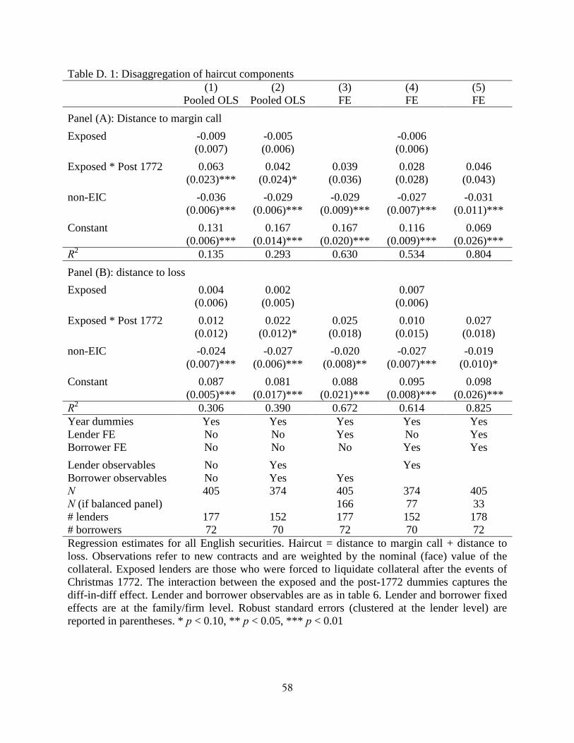
58

Table D. 1: Disaggregation of haircut components (1) (2) (3) (4) (5) Pooled OLS Pooled OLS FE FE FE Panel (A): Distance to margin call Exposed -0.009 -0.005 -0.006 (0.007) (0.006) (0.006) Exposed * Post 1772 0.063 0.042 0.039 0.028 0.046 (0.023)*** (0.024)* (0.036) (0.028) (0.043) non-EIC -0.036 -0.029 -0.029 -0.027 -0.031 (0.006)*** (0.006)*** (0.009)*** (0.007)*** (0.011)*** Constant 0.131 0.167 0.167 0.116 0.069 (0.006)*** (0.014)*** (0.020)*** (0.009)*** (0.026)*** R2 0.135 0.293 0.630 0.534 0.804 Panel (B): distance to loss Exposed 0.004 0.002 0.007 (0.006) (0.005) (0.006) Exposed * Post 1772 0.012 0.022 0.025 0.010 0.027 (0.012) (0.012)* (0.018) (0.015) (0.018) non-EIC -0.024 -0.027 -0.020 -0.027 -0.019 (0.007)*** (0.006)*** (0.008)** (0.007)*** (0.010)* Constant 0.087 0.081 0.088 0.095 0.098 (0.005)*** (0.017)*** (0.021)*** (0.008)*** (0.026)*** R2 0.306 0.390 0.672 0.614 0.825 Year dummies Yes Yes Yes Yes Yes Lender FE No No Yes No Yes Borrower FE No No No Yes Yes Lender observables No Yes Yes Borrower observables No Yes Yes N 405 374 405 374 405 N (if balanced panel) 166 77 33 # lenders 177 152 177 152 178 # borrowers 72 70 72 70 72 Regression estimates for all English securities. Haircut = distance to margin call + distance to loss. Observations refer to new contracts and are weighted by the nominal (face) value of the collateral. Exposed lenders are those who were forced to liquidate collateral after the events of Christmas 1772. The interaction between the exposed and the post-1772 dummies captures the diff-in-diff effect. Lender and borrower observables are as in table 6. Lender and borrower fixed effects are at the family/firm level. Robust standard errors (clustered at the lender level) are reported in parentheses. * p < 0.10, ** p < 0.05, *** p < 0.01

59

East India Stock only

In the baseline results, we use lending against all assets in our database – East India stock (EIC),

3% annuities, and Bank of England stock. While we control for compositional change, it is

interesting to examine how much of a shift we can find by focusing on EIC stock exclusively

(the asset against which the Seppenwolde syndicate predominantly borrowed).

In Table D. 2, panel A, we show that lending requirements in EIC stock changes in very

much the same fashion as in the universe of all assets. In the pooled estimation (col 2), the

coefficient suggests a rise in collateral requirements by 6.8 percent. The fixed effect estimates

look very similar to the benchmark numbers in . However, estimates become (borderline)

insignificant. This is because with fixed effects, the effective number of observations that can be

used to identify the interaction effect is constrained to those that are in the sample before and

after 1772. In addition, we lose observations by constraining the sample to EIC transactions.

In panel B, we analyze lending against non-EIC assets only. Due to the limited number of

observations, the fixed effect specifications cannot be estimated. The pooled OLS estimates are

very similar to those for loan contracts collateralized with EIC stock. For example, the estimate

of the interaction effect in col 2 is 6.6% (versus 6.8% in panel A). Overall, there is no reason to

think that the estimated effects in our baseline specification only reflect changes in haircuts in

one type of asset.

60

Table D. 2: Haircuts – different types of collateral (1) (2) (3) (4) (5) Pooled OLS Pooled OLS FE FE FE Panel (A): EIC only Exposed -0.002 0.000 0.004 -0.000 0.015 (0.008) (0.008) (0.019) (0.008) (0.016)

Exposed * Post 1772 0.072 0.068 0.074 0.037 0.055 (0.025)*** (0.028)** (0.045) (0.026) (0.044)

Constant 0.222 0.240 0.225 0.210 0.169 (0.006)*** (0.016)*** (0.032)*** (0.013)*** (0.046)*** N 314 288 314 288 314 N (if balanced panel) 134 65 41 # lenders 147 127 147 127 147 # borrowers 60 57 60 57 60 R2 0.132 0.296 0.561 0.599 0.787 Panel (B): BoE, SSC and 3% Annuities Exposed -0.007 -0.005 (0.008) (0.007)

Exposed * Post 1772 0.102 0.066 (0.016)*** (0.027)**

Constant 0.158 0.226 (0.007)*** (0.019)*** N 104 99 # lenders 70 64 # borrowers 27 26 R2 0.072 0.284 Year dummies Yes Yes Yes Yes Yes Lender FE No No Yes No Yes Borrower FE No No No Yes Yes Lender observables No Yes Yes Borrower observables No Yes Yes Regression estimates for EIC and BoE, SSC and 3% Annuities separately. Observations refer to new contracts and are weighted by the nominal (face) value of the collateral. Haircuts are calculated as the fraction of the collateral value that is not financed with a loan. Exposed lenders are those who were forced to liquidate collateral after the events of Christmas 1772. The interaction between the exposed and the post-1772 dummies captures the diff-in-diff effect. Lender and borrower observables are as in table 6. Lender and borrower fixed effects are at the family/firm level. Due to a limited number of observations the fixed effects models cannot be estimated for the non-EIC securities. Robust standard errors (clustered at the lender level) are reported in parentheses.* p < 0.10, ** p < 0.05, *** p < 0.01

61

Outliers

It is possible that a few, extreme values for the haircuts influence our results. A standard way to

deal with this issue is to winsorize the data. We winsorize the top and bottom 5 percent of

observations, and re-estimate (see Table D. 3). The results are largely unchanged. Coefficients

are significant throughout, and are statistically indistinguishable from those in the baseline

specification. For completeness we do the same for interest rates and reestimate our benchmark

results . Again, results are virtually unchanged.

Table D. 3: Haircuts – Winsorized dependent variable (1) (2) (3) (4) (5) Pooled OLS Pooled OLS FE FE FE Exposed -0.005 -0.003 -0.001 (0.005) (0.004) (0.006) Exposed * Post 1772 0.072 0.064 0.060 0.040 0.059 (0.020)*** (0.022)*** (0.032)* (0.022)* (0.031)* Non-EIC -0.057 -0.054 -0.047 -0.051 -0.045 (0.006)*** (0.006)*** (0.011)*** (0.008)*** (0.014)*** Constant 0.219 0.240 0.236 0.214 0.199 (0.006)*** (0.014)*** (0.022)*** (0.011)*** (0.033)*** R2 0.369 0.470 0.677 0.655 0.842 Year dummies Y Y Y Y Y Lender FE N N Y N Y Borrower FE N N N Y Y Lender observables N Y Y Borrower observables N Y Y N 418 387 418 387 418 N (if balanced panel) 166 77 33 # lenders 177 152 177 152 177 # borrowers 72 70 72 70 72 Regression estimates for all English securities. Observations refer to new contracts. Haircuts are calculated as the fraction of the collateral value that is not financed with a loan. Exposed lenders are those who were forced to liquidate collateral after the events of Christmas 1772. The interaction between the exposed and the post-1772 dummies captures the diff-in-diff effect. Observations are weighted by the nominal (face) value of the collateral; the top and bottom 5% of the haircut distribution are Winsorized. Lender and borrower observables are as in table 6. Lender and borrower fixed effects are at the family/firm level. Robust standard errors (clustered at the lender level) are reported in parentheses. * p < 0.10, ** p < 0.05, *** p < 0.01

62

Extreme observations

The final step is to examine the sensitivity of our results to the influence of a single lender or

borrower. To this end, we re-estimate the baseline specification (Table 7, col 2), dropping one

lender or borrower at a time. Figure D. 1 panels A-D shows the distribution of coefficients (first

row) and t-statistics (second row). The range of estimated coefficients is small, with results

ranging from 5.5 to 7.5 percent. The t-statistics never falls below 2. This shows that our results

are not driven by a single lender or borrower.

Figure D. 1: Outlier analysis, dropping one lender (borrower) at a time

Dropping one lender at a time Dropping one borrower at a time

(A) Coefficient estimate (B) Coefficient estimate

(C) t-statistic (D) t-statistic

Coefficients on the interaction effect and t-statistics are generated dropping one lender (or borrower) at a time. All estimates include lender and borrower observables.

020

4060

80de

nsity

.05 .055 .06 .065 .07 .075coef. estimate of interaction effect

050

100

150

200

250

dens

ity

.05 .055 .06 .065 .07 .075coef. estimate of interaction effect

0.5

11.

52

2.5

dens

ity

2.2 2.4 2.6 2.8 3 3.2t-stat of interaction effect

01

23

4de

nsity

2 2.5 3 3.5t-stat of interaction effect

Appendix E: Mathematical Proofs

Proof. of Proposition 1. A borrower’s expected profit from a risk free loan l∗j (for j = 1, 2)

is given by

E[Π | lj = l∗j ] = q∗j (v3 − p)where q∗ is the total number of assets a type 3 agent can purchase after obtaining loan

l∗j = rj . Plugging in for c = q∗j (p− rj) we obtain

E[Π | lj = l∗j ] =c

p− rj(v3 − p) (3)

Consider lj > rj . For a lender j to make zero expected returns from his perspective

(remember that by assumption borrowers hold all bargaining power) the interest rate ρ is

set as

ρ(lj) =lj − rjlj

(4)

First consider a loan size l̂j so that the borrower does not expect to default in the the

bad state. In this case the borrower’s expected profits are given by

E[Π | lj = l̂j] =c

p− l̂j

[v3 − p− ρ(l̂j)l̂j

](5)

After plugging in for ρ(lj) the difference between profits (5) and (3) can be written as

E[Π | lj = l̂j]− E[Π | lj = l∗j ]

=c(

p− rj)

(p− l̂j)

[(p− rj

) (v3 − p− l̂j + rj

)+(p− l̂j

)(v3 − p)

]=

c(p− rj

)(p− l̂j)

(l̂j − rj)︸ ︷︷ ︸>0

[(v3 − r) + 2(vj − p)]︸ ︷︷ ︸<0

< 0

where vj − p < 0 follows directly from the assumption that agents of type j do not want

to hold the asset directly.

Next consider the case of a loan size l̃j so that the borrower does expect to default in

the the bad state. Then (after plugging in for ρ(lj)) we arrive at

E[Π | lj = l̃j] =c

2

[1

p− l̃j

(r − p− l̃j + rj

)− 1

]=

c

2

1

p− l̃j

(r + rj − 2p

)=

c

p− l̃j︸ ︷︷ ︸>0

(vj − p)︸ ︷︷ ︸<0

< 0

63

Proof. of Proposition 2. We first describe the equilibrium.

(1) Asset holdings.

Denote by qj the asset holdings of a borrower who is either matched with a type 1 or

2 lender (q1, q2) or is not matched at all (q0, for which we introduce l0 = r0 = 0). From

Proposition 1 it follows that

qj =c3

p− rj, j = 0, 1, 2

where q0 < q1 < q2.(2) Value functions

The value functions of obtaining a loan of type j = 0, 1, 2 are given by

V0 = πq0(v3 − p) + (1− π)

[µ

(N1

N1 +N2V1 +

N2N1 +N2

V2

)+ (1− µ)V0

](6a)

V1 = πq1(v3 − p) + (1− π) [λV0 + (1− λ)V1] (6b)

V2 = πq2(v3 − p) + (1− π) [λV0 + (1− λ)V1] (6c)

where V2 > V1 and where we focus on the situation where V0 ≤ V1.(3) Flow equations and market clearing

Expression (1) in the proposition is the steady state flow equation which equates the

number of new matches to the number of matches that are ended. Expression (2) states

that, in proportion to their importance in the total population, type 1 and 2 agents are

equally likely to be found by a borrower. Solving for Mj gives

Mj =Ni

N1 +N2

µ

µ+ λN3 (7)

Asset market clearing gives

1 = M0q0 +M1q1 +M2q2 (8)

where M0 = N3 −M1 −M2. This implicitly defines price p. Together these expressions

fully describe the equilibrium.

We then proof the Proposition.

Denote

θ1 =N1

N1 +N2

θ2 =N2

N1 +N2

We use these expressions to simplify the value functions V0 and V1. Start with V0 in (6a).

Noting that θ1 + θ2 = 1 and summing V1 (6b) and V2 (6c) we get that

θ1V1 + θ2V2 =π(v3 − p) (θ1q1 + θ2q2) + (1− π)V0

1− (1− π)(1− λ)

64

The expression for V0 can be then restated as

V0 = πq0(v3 − p) + (1− π) [µ (θ1V1 + θ2V2) + (1− µ)V0]

= (v3 − p)q0(π + λ(1− π)) + µ(1− π)(θ1q1 + θ2q2)

π + (λ+ µ)(1− π)

In a similar fashion

V1 =πq1(v3 − p) + (1− π)λV0

λ+ π − λπThe condition V0 ≤ V1 can be written as

V0 ≤ q1(v3 − p)

Which is equivalent to the following condition

q0(π + λ(1− π)) + µ(1− π)(θ1q1 + θ2q2)

π + (λ+ µ)(1− π)< q1 (9)

We use our flow expression (7) and market clearing (8) to simplify. In comination with the

flow equation, market clearing can be written as

q0λN3λ+ µ

+ θ1q1µN3λ+ µ

+ θ2q2µN3λ+ µ

= 1

q0λ+ (θ1q1 + θ2q2)µ =λ+ µ

N3

θ1q1 + θ2q2 =λ+ µ

µN3− c3p

λ

µ

Plugging this into condition (9) and noting that qj = c3p−rj we arrive at

π c3p

+ (1− π)λ+µN3

π + (λ+ µ)(1− π)<

c3p− r1

Denote the likelihood ratio φ = π1−π . Then this condition can be rewritten as

p2 − (r1 +N3c3) p−φN3c3λ+ µ

< 0

This quadratic formula only has one positive root that defines p. The quadratic is U-shaped.

This means that the statement is negative iff p < p.

Proof. of Lemma 1.

Denote

hj = 1−rjp

65

This implies that

δh1δr1

= −p− r1 δpδr1

p2

Since r1 < p this means that δh1δr1

< 0 if δpδr1

< 1. Market clearing (8) implies that

1

c3=M0

p+

M1

p− r1+

M2

p− r2Implicit derivation yields

0 <δp

δr1=

[1 +

M0

M1

(p− r1)2

p2+M2

M1

(p− r1)2

(p− r2)2

]−1< 1

Similarly,δh2δr1

=r2p

δp

δr1> 0

Proof. of Lemma 2.

The first part of this Lemma works purely through prices.

δhjδN3

=rjp2

δp

δN3

Noting that

M0 +M1 +M2 = N3

it is straightforward to see from the market clearing condition that

δp

δN3

> 0

Secondly, note that

h1 − h2 =r2 − r1p

so thatδ (h1 − h2)

δN3

< 0

66

67

Appendix F: Primary Sources GAR: Gemeentearchief Rotterdam (City Archives Rotterdam); NA: Nationaal Archief (Dutch

National Archives); OSA: Oud Archief van de Stad Rotterdam (Old Archives City of Rotterdam); SAA: Stadsarchief Amsterdam (City Archives Amsterdam)

SAA (library), ‘Stukken betreffende den boedel van Clifford en Zoonen’, 1773-1779 SAA, Notariële protocollen Daniel van den Brink, 5075: 10,593 - 10,613 (various notary

protocols) SAA, Tex den Bondt aanvulling 1 en 2, 30269: 347 (‘Staat en inventaris van de boedel van

Johannes van Seppenwolde’) SAA, Archief van de Stads Beleenkamer, 5043: 1 (‘Notulen van de vergaderingen van het

‘Fonds tot maintien van het publiek crediet’ (1773)’) NA, Archief van de familie Van der Staal van Piershil, 3.20.54: 381, 386, 396 (various

correspondence) OSA, 1.01: 3710 (‘Stukken betreffende de kasgeldlening groot fl. 300.000 door de stad aan J. en

H. van Seppenwolde, kooplieden te Amsterdam’) GAR, Archief van de Maatschappij van Assurantie, Belening, etc., 199: 5, 40, 354 (various

accounts and letters) GAR, Archief van Kuyls Fundatie, 90: 52, 56 (various letters) De Koopman, Vol. IV ( 1772-1773) (Dutch periodical)