(Job Market Paper)

Anticipating Takeovers and their Payment Methods:A New Approach Using U.S. Acquisitions

Mohammad Irani ∗

First version : September 08, 2013

This version : November 10, 2015

ABSTRACT

This paper introduces a new approach for identifying the dates on which the market anticipates

both takeovers and their payment forms, prior to their announcement dates. This approach

predicts that the variance-covariance of the stock returns shifts when the market is informed by

signals about potential takeovers with synergistic gains. Using a sample of acquisitions between

U.S. public firms, I find that 86% of takeovers (62% of payment forms) are anticipated on

average nine (six) months in advance. This is much earlier than reported by previous studies

(two months). Moreover, when I add anticipation dates to the cross-sectional determinants of

payment methods, some of the preceding results change. The reason for this finding is that the

firm characteristics are not only related to the choice of payment method but also to the extent

to which takeovers are anticipated.

JEL classification: G14; G17; G34

Keywords: Mergers and acquisitions, payment method, prediction, structural breaks, variance,

covariance

∗The author is a PhD candidate in Finance at Stockholm Business School, Stockholm University, SE-10691 Stockholm, E-mail:mir@sbs.su.se, https://sites.google.com/site/movairani/. I would especially like tothank my supervisors Lars Norden and Rickard Sandberg for their helpful comments and numerous discussions.I am grateful for comments from Chris Adcock, Thomas Bates, Mariassunta Giannetti, Michael Halling, MartinHolmen, Catalin Starica, Johan Stennek, and Joakim Westerlund. I also thank seminar discussants and partici-pants at the second National PhD Workshop in Finance (Stockholm, 2013), the 3rd PhD Conference (StockholmUniversity, 2014), the 63rd Annual Meeting of the Midwest Finance Association (Orlando, 2014), the 23rd AnnualMeeting of the European Financial Management Association (Rome, 2014), Stockholm Business School (2015),and the Annual Meeting of Financial Management Association (Orlando, 2015). I am gratefully acknowledge theJan Wallander and Tom Hedelius foundation for research support. Any errors are my own.

1 Introduction

Jensen and Ruback (1983) and Martynova and Renneboog (2008) review takeover studies

and report that the target shareholders gain large abnormal returns while the returns to the

acquiring firms are negligible (or even negative). Travlos (1987) and Schwert (1996) also doc-

ument that gains in cash-financed offers exceed those in equity-financed and mixed-financed

offers. These differential returns induce investors to try to profit from anticipating takeovers

and their payment forms. The extant studies provide cross-sectional predictions, which provide

no guidance about anticipation dates.1 However, identifying those dates can have important

implications for our understanding of takeovers. Edmans, Goldstein, and Jiang (2012) explain

that stock prices of merging firms are endogenous as they are contaminated with takeover an-

ticipations. The dates can hence be used to remove the effect of takeover anticipation on prices,

which in turn can improve measurement of explanatory variables that use stock prices (e.g., To-

bin’s Q, price-earnings ratio, the discount rate, the acquisition stock returns, return variance,

covariance and correlation of merging stocks). The aim of this paper is to investigate whether

the market can anticipate mergers and acquisitions (M&As) and their payment methods prior

to their announcement dates. If so, when do those anticipations occur, and what are their

consequences for the choice of payment method in M&As?

Detecting the dates on which M&As are anticipated is a challenging task. Li and Prabhala

(2007) argue that M&As occur neither randomly nor unexpectedly, but takeover studies provide

indirect evidence regarding ex-ante predictability of M&As. Schwert (1996) shows that the

cumulative average abnormal returns (CAARs) to the target shareholders start to accumulate

42 trading days before the announcement date. He finds that there is a one-for-one relation

between this pre-announcement run-up and the total premium paid to the target shareholders

(the sum of run-up and post-announcement markup returns). Based on this result, Schwert

concludes that the target pre-announcement run-up is not affected by takeover anticipations,

otherwise it should not be added to the total premium paid by acquirers. However, Betton,

Eckbo, Thompson, and Thorburn (2014) illuminate that the relation is significantly smaller

after they account for the anticipation effect on the target run-up. Overall, findings of event

studies suggest that the market anticipates the target firms on average two months in advance,

but the acquirers are unpredictable because their CAARs do not show any trend in the pre-

announcement period.2 Furthermore, the event-study methodology focuses on just one of the

pair of firms at a time (either the target or the acquirer firm), thereby neglecting the additional

information contained in their joint return distribution (e.g., the covariance), which might be

useful for anticipating M&As. To deal with the unpredictability issue, this paper introduces a

new time-series and direct approach for identifying both the deal-anticipation (a pair of target

and acquirer firms) and payment-form-anticipation dates. This approach is based on analyzing

1Amihud, Lev, and Travlos (1990), Hasbrouck (1985), and Martin (1996), among others, employ a cross-sectional (binary discrimination) approach to examine investors’ predictions of acquirer and target merger can-didacy and their predictions of payment methods.

2Similarly, Smith and Kim (1994) find that the CAARs of the target firms in their sample start accruing 60days before the announcement day; however, the returns to the acquiring firms do not deviate from zero in thisperiod. I find comparable CAARs to theirs for the target and acquirer firms in my sample.

1

breaks in the variance-covariance structure of the joint target and acquirer daily return series.

Betton et al. (2014) suggest that M&As are anticipated when the market receives infor-

mative signals about potential takeovers with synergistic gains. Accordingly, when the market

anticipates a potential deal for the first time during the pre-announcement period, the merging

likelihood should increase significantly. Simultaneously, the market also discounts the expected

synergy value of that merger and incorporates it into the price process of the merging firms,

which in turn can affect the moments of the stocks’ returns (including levels, variances, co-

variance, etc.). The merging likelihood and the expected synergy are generally unobservable,

while shifts in the second-order moments can be estimated, allowing the anticipation dates to be

identified. Not every shift during the pre-announcement period, however, is related to takeover

anticipation. Restrictions are imposed on the sign of shifts in the variance-covariance structure

to disentangle consistent from inconsistent ones. A break date is interpreted as an anticipation

date if shifts around that date are consistent with the expected ones. The expected shift for

the anticipation of a deal is a significant decline in the target’s variance and any significant

changes in the rest of the moments (the acquirer’s variance, the acquirer-target covariance, or

the acquirer-target correlation) during the pre-announcement period. Anticipating the payment

form requires the correlation and (or) the covariance to shift upwards in the case of equity offers

and shift towards zero in the case of cash offers.

This paper contributes to the M&A literature by documenting anticipation shifts. Using

a sample of 125 completed acquisitions of U.S. public companies between 2003 and 2006, the

proposed approach finds that a takeover is anticipated on average 187 trading days before the

announcement date in 86% of the deals. The market anticipates the payment form in 62% of

the deals on average 123 trading days in advance. The anticipation dates that are identified are

much earlier than in previous event studies (e.g., Schwert, 1996) that find only the target (and

not the acquirer) firms to be anticipatable, and just two months prior to the announcement

date. The results suggest that breaks in the variance-covariance structure reveal significant

information about future M&As. Moreover, splitting the sample based on the offered payment

form (54 cash, 33 equity, and 38 mixed-payment deals) indicates that the market anticipates

the cash offers almost at the same time as it anticipates the deals themselves, but on average

there is a lag of 90 trading days in the equity and mixed subsamples. This evidence reveals

that the announcement of cash (equity and mixed) offers contains the least (most) unexpected

information for market investors. The market is less successful in anticipating mixed offers

because this requires the forecasting of an additional parameter, i.e. the portion of cash in the

total bid payment.

Additionally, controlling the deal-anticipation and payment-form-anticipation dates in this

paper provides new insights into the choice of payment method in M&As.3 The first and second-

order moments of the target and acquirer stock returns are used as cross-sectional predictors

in the payment-method regressions. Among them, the correlation plays an important role

in explaining the choice because it is a proxy for the relatedness of the target and acquirer

3Various competing hypotheses (the asymmetric information, tax consideration, capital structure, managerialcontrol, and behavioral motives, among others) explain this choice. See, for instance, Martin (1996) and Betton,Eckbo, and Thorburn (2008) and the references therein.

2

businesses. However, previous findings are mixed. On the one hand, Houston and Ryngaert

(1997), Officer (2004), and Bhagwat and Dam (2014) find that, if the stand-alone target and

acquirer stock prices co-move (are highly correlated), offering equity as the medium of payment

reduces the risk of an “unfair” merger, i.e., one in which the terms of the merger become

“unfair” to one party at the deal completion date. On the other hand, Faccio and Masulis

(2005), Rhodes-Kropf and Viswanathan (2004), and Aggarwal and Baxamusa (2013) argue

that the acquirer should pay in equity when buying uncorrelated target firms if those targets

have an informational disadvantage in that the acquirer’s stock is overvalued. Consistent with

the first of the above strands, I find that the greater the pre-merger correlation, the larger is

the fraction of the acquirer’s equity in the bid payment. However, adding new variables (i.e.

the deal-anticipation and payment-form-anticipation dates) to this regression changes some of

the previous results. Namely, the significance of the correlation disappears, the coefficient of

the average target return becomes significant, and the coefficient of the target volatility is

attenuated.

The above evidence suggests that assuming the unpredictability of M&As in payment-

method regressions may result in some endogeneity issues. First, the moments are usually

estimated from the pre-announcement period, but the anticipation of M&As can affect them.

The moments hence need to be estimated from a period in which the takeovers are totally unex-

pected (i.e. from the pre-anticipation segment); otherwise, they might be mismeasured, which

in turn may lead to a “measurement error” in the regressions. In fact, the evidence here indi-

cates that the pre-announcement target and acquirer variances are underestimated compared

with those from the pre-anticipation period. Similarly, the covariance and correlation are un-

derestimated in cash offers and overestimated in equity offers. Second, the target, acquirer, and

acquisition characteristics are used as predictors in those regressions. My findings demonstrate

that the anticipation variables are significantly correlated with some of those characteristics,

making them relevant for inclusion in the regressions. In other words, excluding the anticipation

variables may cause “omitted-variable bias”. My results indeed confirm that this is the case, at

least for my sample of takeovers.

I find robust support in the data for two theoretical factors (merging likelihood and expected

synergy) that generate the anticipation shifts. Using a measure for the takeover probability

(from Samuelson and Rosenthal, 1986), the merging likelihood of the target and the acquirer

firms become significant for the first time during the pre-announcement period after the detected

deal-anticipation dates, and then trend upwards. Moreover, the CAARs of both the target

and acquirer shares also show positive and significant trends after those anticipation dates,

suggesting that the market discounts part of the expected synergy of future M&As around

those dates. These findings confirm the assumptions in the theoretical model of Betton et al.

(2014), in which takeovers are anticipated when the market is informed by strong signals about

potential takeovers with synergistic gains.

I perform robustness tests in an attempt to rule out several alternative explanations of the

results: (1) If those anticipation shifts are caused by firm-specific events (and not anticipation

of M&As), then the portfolio theory would suggest that the variance-covariance structure of the

3

portfolios of merging firms should be stable due to the diversification effect. However, I also find

similar shifts in the variance-covariance structure of the portfolios, indicating that firm-specific

news is not the source of anticipation shifts in the individual bivariate return series. (2) If

some market-wide events during the sample period of this paper cause those anticipation shifts,

then similar shifts should also be observed in a benchmark sample (i.e., a random sample of

non-M&A firms). The anticipation shifts occur much less frequently and in a less expected way

in the benchmark sample than in the M&A sample, implying that the likely mechanism for the

later shifts is anticipation of takeovers and not market-wide events.4

I also apply cross-sectional analyses to determine the significant predictors that explain why

some takeovers are anticipated and some not, and why some are anticipated earlier than others.

I find that some of the cross-sectional characteristics of merging firms in the pre-anticipation

segment are significant in discriminating anticipated from unanticipated deals and in explain-

ing cross-sectional variation in the anticipation dates. While Meulbroek (1992) and Schwert

(1996) consider leakage of information by insiders as the main source of M&A anticipation, my

results propose another source: the existence of M&A anticipators in the market who use public

information that is available prior to the deal-anticipation date to predict likely M&As.

The rest of the paper is organized as follows: Section 2 reviews the merger arbitrage literature

to identify expected shifts that signal the anticipation of takeovers. Section 3 presents the

methodology and the anticipation hypotheses. Section 4 provides data and descriptive statistics.

Section 5 documents the anticipation results. Section 6 discusses the robustness of the results.

Section 7 reports the cross-sectional results, and finally Section 8 concludes.

2 Anticipation Shifts

According to the efficient market hypothesis (EMH), all relevant information should be

instantly incorporated into stock prices. Therefore, if the market anticipates a takeover and its

payment method, this information should be reflected in the price process of the target and the

acquirer stocks at the anticipation time. The merger arbitrage literature documents changes in

the second-order moments of stock returns after the announcement of takeovers. If the market

is efficient, one can expect to observe similar changes during the pre-announcement period when

a deal and (or) its payment form are anticipated.

The expected shifts that would indicate the anticipation of the deal and payment form can be

summarized as follows: a significant decline in the target volatility indicates the anticipation of

the target firm while any significant shift in the acquirer’s volatility would imply the anticipation

of the acquirer firm. The existence of a significant decline in the target’s variance and of any

significant changes in the rest of the moments (the acquirer’s variance, the acquirer-target

covariance, or the acquirer-target correlation) during the pre-announcement period signal the

anticipation of the takeover. If the market anticipates equity offers, the covariance should

4The anticipation shifts exist regardless of the use of alternative approaches. The alternatives include thefollowing: three univariate tests as opposed to one multivariate test for detecting breaks in the variance-covariancestructure, the use of raw instead of winsorized returns series, and the employment of returns from the pre-announcement period rather than from both the pre- and post-announcement periods in the above tests.

4

increase and (or) the correlation should become one. In the case of cash offers, the covariance

and (or) the correlation should converge to zero. A mixed-payment offer will follow the rule for

equity (cash) offers if the equity (cash) is the dominant portion in the total bid payment.

2.1 Target Return Volatility

Bhagat, Brickley, and Loewenstein (1987) report an anomaly in the relation between risk and

return in targets’ stocks during the post-announcement period. They find significant declines

in both the beta and the sample unconditional volatility of the target of a cash bid, but rising

returns. Bhagat et al. (1987) propose that the price of a target share during that period is the

sum of the value of common stock and the value of a put option. The target shareholders have

the option to sell their shares to the acquirer firm in the post-announcement period. Bhagat et

al. (1987) then show via option theory that a portfolio containing a stock and a put option has

a lower standard deviation than the stock itself. This conjecture explains the observed decline

in the target’s volatility.

Hutson and Kearney (2001, 2005) extend this analysis to the targets of both cash and equity

offers and to completed and failed ones. They document that, regardless of the payment form

and the final outcome of the pending bid-offer, the conditional volatility of the target’s shares

declines significantly after the bid announcement. The greatest (smallest) decline is in the

cash (equity) subsample. Hutson and Kearney (2001) claim that this observation is due to a

fundamental change in the price formation process, i.e. traders’ opinions about the value of the

target stock converge during the post-announcement period. Overall, the decline in the target

volatility regardless of the payment method and the offer outcome indicates an increase in the

likelihood of a firm being the target of an acquisition.

2.2 Acquirer Return Volatility

Various competing hypotheses have been developed about the post-acquisition (i.e., long-

run) risk profile of the acquirers. First, the “portfolio effect” hypothesis predicts that the risk of

the acquiring firm in this period is nothing more than the risk of a market-value-weighted port-

folio formed from the shares of the two firms in the pre-announcement period (e.g., Langetieg,

Haugen, and Wichern, 1980), thereby suggesting a decline in its risk. Second, the “leverage

effect” hypothesis expects acquisitions that worsen the leverage (debt-to-equity ratio) of the

acquirer firm to induce an increase in the risk of the consolidated firm (Hamada, 1972). Third,

the “integration risk” hypothesis conjectures an increase in the risk of the consolidated firm

if the acquirer’s management is inefficient in merging the two firms into a single corporation

(Bharath and Wu, 2006). Fourth, the “merger wave effect” hypothesis posits that industry

shocks trigger inter-industry acquisitions (Mitchell and Mulherin, 1996; Harford, 2005). Since

completed inter-industry acquisitions have stabilizing effects, this hypothesis predicts a decline

in the risk of the consolidated firm. Finally, the “synergy effect” hypothesis predicts a decline

in the acquirer’s risk since the synergistic gains increase the value of the consolidated firm due

to the following reasons: cost reductions due to economies of scale, economies of scope, more di-

5

verse corporate skills, more efficient redeployment of the combined assets, and enhanced market

power, among others (e.g., Bradley, Desai, and Kim, 1988; Chatterjee and Lubatkin, 1990).

Given the opposing predictions, the net impact of acquisitions on the risk of the acquirer

firm is an empirical question. The empirical findings are indeed mixed. For example, Langetieg

et al. (1980) show an increase in various unconditional risk measures of the acquirers in the

post-acquisition period. They relate this result to aggressive management of the acquirer firms

together with an increase in their leverage. Geppert and Kamerschen (2008) find a statistically

greater implied volatility of the acquirer firms than the value predicted by the portfolio hypoth-

esis in the post-announcement period. They argue that the integration risk and uncertainty

about potential efficiency gains explain this result. However, after controlling for the system-

atic risk of target firms, Chatterjee et al. (1990) find the acquirers’ systematic risk to decline

over both short and long horizons after the acquisitions due to synergistic gains. Hutson and

Kearney (2005) find that the average unconditional volatility of the acquiring firms declines

significantly after the announcements, but that the reduction is only significant in cash offers.

Declining shifts are more consistent with the proposed anticipation mechanism in which a

takeover is anticipated if the market perceives a synergistic gain from the merger. A decline in

the acquirer risk during the pre-announcement period hence suggests that the diversification and

synergy effects dominate the leverage and integration impacts. Overall, the opposing hypotheses

and mixed evidence predict changes in the acquirer risk in different directions. Therefore, any

change in the pre-announcement period is interpreted in this paper as an indicator of the

anticipation of the acquirer firm.

2.3 Acquirer-Target Return Correlation

Houston et al. (1997), Officer (2004), and Bhagwat et al. (2014) report a positive relation

between the fraction of the acquirer’s equity in the bid payment and the pre-announcement

correlation. Bhagwat et al. (2014) propose that the risk of overpayment is reduced by an equity

offer if the acquirer and target returns are highly correlated but the risk increases with weak

correlation. This result suggests that shifts in the correlation can be used to anticipate the

payment method in M&As.

Subramanian (2004) constructs a theoretical model and provides empirical evidence in which

the announcement of an equity offer causes the correlation to shift towards perfect correlation.

He argues that if the market assigns a high likelihood to the success of a merger attempt, the two

stock price processes must be perfectly correlated after the bid announcement since the acquirer

offers a constant equity-exchange ratio to acquire each share of the target firm in an equity

bid. This paper extends the work by Subramanian (2004) by documenting the behavior of the

correlation around the announcements of cash and mixed-payment offers. When the likelihood

of the success of a cash offer is high, the target volatility should drop significantly due to the

offered bid premium. In this case, the two return processes will become uncorrelated. Moreover,

the proportion of cash in a mixed payment will determine whether the correlation should shift

towards zero or one. If the cash portion is dominant, the above argument predicts that the

correlation should converge to zero. Otherwise, it should shift towards perfect correlation.

6

2.4 Acquirer-Target Return Covariance

The behavior of the acquirer-target return covariance around the announcement of cash,

equity and mixed-payment offers has not been studied previously. This paper does so for the

first time. Both the covariance and the correlation measure the degree of covariation between

the target and acquirer returns. However, standardization via individual volatilities in the

denominator of the correlation can mean that useful variations necessary for anticipating the

payment form are discarded. It is likely that the correlation will be stable, while the covariance

will shift in response to the market’s anticipation of the payment form. This suggests that shifts

in the covariance can be used along with shifts in the correlation to detect the payment-form-

anticipation dates. Overall, the expected shifts in the correlation apply to the covariance as

well.

3 Methodology and Anticipation Hypotheses

First, each return series is prepared (i.e., adjusted for outliers, and for breaks in the mean,

and then demeaned) before the structural break test is applied to investigate whether a deal and

its payment form are anticipated or not. Second, if the test detects break(s) in the variance-

covariance structure of a bivariate return series, the significance of shifts in its second-order

moments are examined individually around each break date. Finally, an inference about the

existence of anticipation dates is made based on the signs of the significant shifts.

3.1 Data Preparation

The daily log returns (henceforth, the returns) of the acquirer and target stocks are used in

all the tests in this paper and are computed in the following way:

ri,n,t = ln

(Pi,n,t

Pi,n,t−1

), (1)

where i =Acq, Trg ; n is the index for the deals in the sample; t=(-379, . . . , 0, 1, . . . , C ) is

the daily subscript; rAcq,n,t and rTrg,n,t represent the realized returns to acquirer and target

shareholders involved in deal n on day t ; and PAcq,n,t and PTrg,n,t are their adjusted closing

prices on day t. Similarly to in Schwert (1996), the sample observation period for each of the

target and acquirer return series starts 379 days prior to the announcement date (t = 0) and

ends at the delisting date of the target’s shares, which is C days after the announcement.5 The

pre (post)-announcement period runs from Day -379 (Day 0) to Day -1 (Day C ).

The largest absolute returns of each series are identified and winsorized at 99%. The mean

of the returns should be stable during the whole observation period in order that breaks in

the second-order moments can be identified. The structural breaks methodology developed by

5The cross-sectional regressions (e.g., Amihud et al., 1990; Hasbrouck, 1985; Martin, 1996) use predictorsfrom the last year to discriminate merging from non-merging firms. Starting the sample observation period atDay -379 (one and a half years before the announcement day) here corresponds to the idea in those papers thatthe relevant information about future M&As can be revealed one year in advance.

7

Bai and Perron (1998, 2003, 2006) detects shifts in the mean of each return series, each series

then being adjusted for the detected shifts. See the “Data Preparation” section in the internet

appendix for further details about the adjustment of outliers and the structural break test. All

tests used in this paper assume the sample mean of each return series to be zero. The following

transformation is therefore applied to each series:

ri,n,t = ri,n,t − ri,n,t, (2)

where ri,n,t =1

380 + C

C∑t=−379

ri,n,t is the sample mean of the observed return series and ri,n,t is

the mean-adjusted return series.

3.2 Detecting Breaks in the Variance-Covariance Structure

I use a cumulative sum (CUSUM) type test proposed by Aue, Hormann, Horvath, and

Reimherr (2009). This test is suitable since it does not impose any normality or parametric

assumptions, which are usually assumed in parametric and cross-sectional tests. However, it re-

quires the finiteness of the fourth sample moment of the bivariate series. The 99% winsorization

is thus necessary and used to fulfill this requirement. The appealing feature of CUSUM-type

tests is their ability to use a non-parametric HAC (heteroskedasticity- and autocorrelation-

consistent) type estimator to capture the dependence structure in the data. As recommended

by Aue et al. (2009), the Bartlett estimator is used as a proxy for the asymptotic covariance

matrix in the testing procedure.6,7

Since shifts in the variance-covariance structure can occur in both the pre- and post-

announcement periods, I use the multiple break detection version of Aue et al. (2009), which is

based on the binary segmentation approach. When this test detects a significant break date, it

is reapplied separately across the two new segments that are obtained from splitting the data

into two subsamples around that break date. This approach ends when the test can no longer

detect any significant breaks in the new segments.

Henceforth, the identity subscript of the deals is excluded from the notation for simplicity,

but the following procedure is applied for each deal in the sample. Let (y−379, . . . , y0, . . . , yC)

be a sequence of two-dimensional random return vectors over the sample observation period of

a deal. For example,

y−379 =

(rAcq,−379

rTrg,−379

)(3)

is the bivariate vector of mean-adjusted realized returns for the target and acquirer shareholders

6Berkes, Horvath, Kokoszka, and Shao (2005) show that the Bartlett estimator to be a consistent estimatorof the asymptotic covariance matrix since it converges almost surely.

7The data-dependent approach of Newey and West (1994) is also applied to determine an optimal truncationlag in the Bartlett estimator. Rodrigues and Rubia (2007) show this truncation lag to be able to improve thefinite-sample performance of CUSUM-type tests.

8

on Day -379.

Cov(y−379) =

(σ2Acq,−379

σ2AcgTrg,−379 σ2Trg,−379

)=

(r2Acq,−379

rAcq,−379.rTrg,−379 r2Trg,−379

)(4)

is the realized variance-covariance matrix of the bivariate returns on Day -379, which contains

the realized target and acquirer variances and their realized covariance on that date. The test

statistic of Aue et al. (2009, p. 4050) detects structural breaks in the variance-covariance

structure of a bivariate return process by examining the following hypotheses:

H0 : Cov(y−379) = . . . = Cov(yC) (5)

HA : Cov(y−379) = . . . = Cov(yK1) 6= Cov(yK1+1) = . . . = Cov(yK2)

6= . . . = . . . 6= Cov(yKm+1) = . . . = Cov(yC). (6)

While the null hypothesis indicates the constancy of the variance-covariance structure of a

bivariate return series in the sample observation period, the alternative allows several change-

points (m ≥ 1). The test itself identifies the unknown number of change-points (m) and their

unknown locations (-379<K1<. . .<Km<C ). I do not impose any restrictions on these unknown

parameters so as to capture all informational events of each bivariate series.

The merger arbitrage literature usually compares the cross-sectional average pre- and post-

announcement second-order moments by assuming the announcement day to be the only break

date (e.g., Bhagat et al., 1987; Hutson and Kearney, 2001; Subramanian, 2004). To the best of

my knowledge, Jayaraman, Mandelker, and Shastri (1991) is the only study that documents pre-

dictability for the target firms by assuming three uniform break dates in their implied volatility

during the pre-announcement period. Gelman and Wilfling (2009) apply a Markov-switching

GARCH model to detect shifts in the conditional volatility of target stocks during the post-

announcement period. However, the use here of the test provided by Aue et al. (2009) extends

the above studies because it relaxes any assumptions about the number and location of break

dates.

3.3 Tests for Equality of Second-Order Moments around the Break Dates

Since Aue et al.’s (2009) test is a joint test, it does not identify which of the second-

order moments changes significantly after each break date, knowledge of which is necessary in

order to examine the anticipation hypotheses. Therefore, I perform tests for the equality of

those moments to determine significant shifts after each break. Since the sample second-order

moments are locally stationary in each segment, I use them as estimates for the population

moments across the detected segments. Suppose, e.g., that the joint test finds one break in the

variance-covariance structure at time K1. Then the estimates of the target’s variance in the

9

pre- and post-break segments are

σ2Trg,pre =1

(379 +K1)

K1∑t=−379

r2Trg,t (7)

σ2Trg,post =1

(C −K1)

C∑t=K1+1

r2Trg,t. (8)

Other sample second-order moments (i.e., acquirer variance, covariance and correlation) in

the pre- and post-break segments are estimated in a similar way.

The modified version of Levene’s (1960) F-test, proposed by Brown and Forsythe (1974),

examines whether the sample variance is the same across two adjacent segments. This test

is proper since it uses the median instead of the mean in computing the absolute deviations,

and thereby robust against non-normality.8 For example, this test examines whether the target

variance is constant around a break date:

H0 : σ2Trg,pre = σ2Trg,post (9)

HA : σ2Trg,pre 6= σ2Trg,post. (10)

The F-statistic is always positive, but the covariance can be negative. Thus, the absolute

value of the covariance is used here for computing the common F-test for the equality of co-

variances across two adjacent segments. However, using absolute values can lead to a more

conservative test in detecting heterogeneity when the sign of the covariance is different in the

two segments. The number of significant changes might hence be underestimated if the absolute

values are small.

Jennrich’s (1970) test examines the equality of sample correlations across two adjacent

segments:

H0 : ρAcqTrg,pre = ρAcqTrg,post (11)

HA : ρAcqTrg,pre 6= ρAcqTrg,post, (12)

where ρAcqTrg,pre and ρAcqTrg,post are the sample acquirer-target return correlation in the pre-

and post-break segments.

3.4 Anticipation Hypotheses

Previous studies document that information about the pair of firms (e.g., the size of the

target relative to the size of the acquirer) explains the choice of payment method in M&As.

Thus, first, the deal anticipation should be examined and then the payment-form anticipation.

If the deal is unanticipated, the procedure for detecting the payment-form-anticipation date is

abandoned. Moreover, the payment form can be anticipated either at the deal-anticipation date

or at a later date during the pre-announcement period.

8Lim and Loh (1996) compare seven existent tests for the equality of variances in a simulation exercise andfind that the modified Levene test is the most powerful.

10

The following conjectures help to interpret the results of the structural break test, and in

turn to detect the anticipation dates. First, the existence of multiple consistent breaks will

indicate that expectations about the potential deal are updated sequentially. Such breaks will

occur due to the release of new information about the deal, the reinterpretation of existing

information, and (or) the reassessment of the perceived synergy of the deal and its division

between the target and acquirer shareholders. Second, assuming a threshold of 50% shows

whether a mixed offer is anticipated or not. Thus, if more than 50% of a deal value is paid in

cash (equity), then cash (equity) is the dominant payment form in the mixed-payment offer.

Table 1 summarizes possible outcomes of the test (by Aue et al., 2009), which are inferred

to identify break date(s) consistent with the deal and payment-form-anticipation hypotheses.

First, if there is no break during the pre-announcement period of a bivariate (target-acquirer)

return series, then the deal and its payment form are unanticipated. Furthermore, non-M&A

reasons can increase the volatility of the target shares. Thus, any increasing shift in this moment

will lead to a break date not being recognized as a deal and payment-form-anticipation date,

regardless of the observation of expected shifts in other moments (see, e.g., outcomes 2 and 5

in Table 1).

Insert Table 1 here

Second, suppose that the test detects only one break date (K1). If at least one of the

second-order moments (other than the target variance) changes significantly after this break,

then K1 is the deal-anticipation date (outcomes 3 and 4). A decline in the target variance may

only indicate that the market anticipates the target firm and not the deal (which is a pair of

target and acquirer firms). Therefore, in addition to a declining target variance, the existence

of at least one significant shift in another moment is required for a break to be considered as

the deal-anticipation date.

The deal-anticipation date is the first candidate for assessing the payment-form-anticipation

hypothesis. If at least one of the covariance and the correlation shifts significantly towards its

expected level after this date, then K1 is also the payment-form-anticipation date. An expected

shift would be a rise in the case of equity offers, or a shift towards zero in the case of cash

offers. A mixed offer would follow the rule for an equity (cash) offer if equity (cash) made up

the dominant portion of the total payment.

Finally, let us assume for simplicity a two-break case (K1 and K2), though this can easily

be generalized to a case with more than two breaks. In the multiple break case, the procedure

starts from the closest break to the announcement date (K2) since it captures the most recent

expectations of the market about the M&A activity of the pair of firms. If there are any

inconsistent shifts (e.g., increasing target variance), then the deal and its payment form are

inferred to be unanticipated (outcomes 5 and 6). However, if K2 contains consistent shifts,

then the anticipation procedure considers the farther break (K1) as well. If there are consistent

break(s) around this date, then the market starts to anticipate the deal and (or) its payment

form from the date of the distant break, i.e., K1 (outcomes 9 and 10), otherwise the deal

and (or) its payment form are anticipated at K2 (outcomes 7 and 8). Moreover, a reversal in

11

the co-movement moments across breaks can cause the deal-anticipation and payment-form-

anticipation dates to differ, and can even cause the payment form to be unanticipated (if an

inconsistent break is detected at the closest break date). If the dates are different, then the deal

is anticipated (K1) earlier than the payment form (K2), e.g., outcomes 11 and 12.

The choice of payment method at the acquisition time can differ from the anticipated one. If

so, then the payment form is found to be unanticipated (anticipated incorrectly). For instance,

according to possible outcomes 3 and 9 (7 and 12), the market anticipates at date K1 (K2)

that the acquirer will use its own shares to finance the acquisition, but if instead it uses cash at

the acquisition time, then the payment form will have been unanticipated. This example shows

cases in which the deal is anticipated but not its payment form. Section 6.1 below provides an

example of how the above procedures are performed so as to identify the anticipation dates.

4 Data and Descriptive Statistics

4.1 Sample Selection

I sample takeovers from the Bureau Van Dijk Zephyr database using the transaction form

of “merger” or “acquisition”. The sample consists of all completed acquisitions between U.S.

publicly listed target and acquirer firms. The sample period is from June 2003 to June 2006,

which corresponds to the sixth M&A wave in which both the equity and the takeover markets

are stable (Martinova and Renneboog, 2008). Macroeconomic and industry factors are less

likely to generate breaks in this period than is the release of information about firms (e.g.,

takeover transactions). This definition leads to 1647 deals being identified. Table 2 summarizes

how this sample is then reduced based on the following filters.

Insert Table 2 here

I focus on the sample of deals in which the following hold: (i) An acquirer gains entire

control of a target firm by acquiring 100% of the target shares in one takeover transaction. The

most relevant cases in which to verify the anticipation mechanism are those in which the ex-ante

merging likelihood is trivial. I thus exclude acquisitions in which an acquirer has acquired some

stake in the target firm before the current bid, because previous bids (of even a minority or

“toehold” stake) can raise the likelihood to a significant level. (ii) The method of payment is all-

cash, all-equity or a mixture of cash and equity payments. (iii) A bid offer takes between 19 and

253 trading days from its first announcement date to complete. According to the William Act

of 1968, only bid offers for subsidiaries of U.S. public targets or private targets can be completed

in a shorter period (Officer, 2004; Bhagwat and Dam, 2014). The daily prices (and thus the

returns) are usually unobservable for these firms, and so the anticipation mechanism would

be unverifiable for these types of deals. (iv) The deal value exceeds $50 million. (v) Neither

the acquirer nor the target firm is a bank since the latter are highly leveraged and subject to

different regulations. The noise that would be added to the estimation of the cross-sectional

regressions due to their different characteristics is the primary reason for ignoring banks. (vi)

An acquirer has only one bid record in the sample period. If an acquirer has multiple bids, a

12

consistent break would not be identifiable as the anticipation break of a specific bid, as it might

be related to another bid made by that acquirer. (vii) The target has a stock price exceeding

$2 on Day -42. Schwert (1996) argues that the returns on low-priced stocks could be imprecise

as they are more heavily exposed to frictions in the market microstructure. (viii) Both firms

have more than 120 adjusted daily-closed stock prices during the pre-announcement period in

Thomson Financial DataStream.

The final sample contains 125 deals with enough return data, and splits into 54 all-cash, 32

all-equity and 38 mixed-payment deals. This sample size might be considered small compared

to the sample of the usual takeover study. The reason is that more restrictive filters are used

here to construct the sample, which is necessary for testing the anticipation hypotheses. For

example, filter (i), requiring bids for a 100% stake of the target, reduces the sample significantly

by 1120 deals, and other studies do not impose this requirement.

The target and acquirer firms’ accounting and deal information are retrieved from Thom-

son Financial DataStream and the Bureau Van Dijk Zephyr database. The internet appendix

provides further details of the data analysis, including the definition of the variables for the

cross-sectional analysis, descriptive statistics of the deal, target and acquirer characteristics,

the sample higher-order moments before and after winsorizing the return series, and the results

for the breaks in the mean returns.

4.2 Summarized Statistics of Sample Second-Order Moments

Table 3 provides descriptive statistics for the sample second-order moments of the acquirer

and target returns in the pre- and post-announcement periods. I use the sample moments

and not the realized moments in order to compare the results with those of previous studies.

The cross-sectional average (median) annual target volatility for the full sample declines by

a highly significant 44.1% (47.1%), from 0.483 (0.463) to 0.27 (0.245), from the pre- to the

post-announcement periods.9 This average decline is similar to Hutson and Kearney’s (2001)

report of an average decline of 46% after the bid announcement. While the analysis of variance

(ANOVA) indicates that the average target volatility is comparable across payment subsamples

during the pre-announcement period, its large F-value (16.28) for the post-announcement period

suggests the opposite. Consistent with Hutson and Kearney (2001), the largest (smallest) risk

reduction is seen for the targets of cash (equity) offers. Overall, the announcement of a takeover

significantly reduces the target’s volatility regardless of the payment method offered. This is

consistent with that part of the deal-anticipation hypothesis that partially anticipates a takeover

due to a significant decline in this moment.

Insert Table 3 here

The decline in the average acquirer volatility is significant at the 1% level. It changes from

0.384 to 0.318 between the pre- and post-announcement periods. Again, this average decline

9I will report the volatilities (and not the variances) throughout the paper for comparability of the resultswith previous literature, and annualize all moments (over 252 trading days) to match them with the annualcross-sectional data used in the regressions.

13

(17.4%) is similar to the 21% drop reported in Hutson and Kearney (2005). This average

reduction in the risk of acquirers after bid announcements is less than that found for the targets

(44.1%) since the above-mentioned opposing factors affect the acquirer’s volatility. Moreover,

the average reduction is significant across all payment subsamples, ranging from 15% to 19%.

Overall, the synergy and diversification effects dominate the leverage and integration effects in

this sample, such that the bid announcements lead to a decrease in the acquirers’ volatility.

The difference between the average post- and pre-announcement covariance is insignificant,

which is surprising at first glance. However, the unreported results of the individual equality

tests indicate that the covariance changes significantly in 110 out of 125 (88% of) deals after the

announcement. The decreasing and increasing changes cancel each other out in this case, causing

the average change to be insignificant. Furthermore, the significant ANOVA results (with F-

values of 5.72 and 22.93) imply that both the average pre- and post-announcement covariance

differ significantly across payment subsamples. The firm-pairs that are more linearly dependent

during the pre-announcement period use more equity as the medium of exchange. Moreover,

consistent with the payment-form-anticipation hypothesis, announcing an equity (cash) offer

significantly raises (declines) the average covariance by 65.7% (99.1%), from 0.066 (0.029) to

0.11 (0.0003), from the pre- to the post-announcement periods. Overall, the covariance changes

significantly after the bid announcement, dependent on the offered payment method.

Consistent with Bhagwat et al. (2014), I find that the more correlated is the pair of firms

in the pre-announcement period, the more shares are used by the acquirer to finance the M&A

(F-value of 8.32). Announcements of equity offers significantly increase the average correlation

from 0.305 to 0.685. This result supports the evidence in Subramanian (2004) in which it is

proposed that the correlation of firm-pairs involved in equity deals should shift upward after

the announcement. The average correlations decline significantly by 84.4% (from 0.17 to 0.026)

after cash announcements. Similarly to in the covariance case, the results for the correlation

are consistent with the expected changes for the anticipation of the payment method.

All in all, the sample post-announcement moments are different from the pre-announcement

ones. The differences are consistent with the previous findings in the literature, showing this

sample to be comparable with previous ones. Moreover, the announcements move the second-

order moments towards the aforementioned expected levels.

5 Evidence on the Anticipation of Deal and Payment Form

5.1 Breaks in the Variance-Covariance Structure

Table 4 and Figure 1 summarize the results of performing Aue et al.’s (2009) test on the

125 bivariate return series. There is at least one significant break in 87.2% of the deals (109 out

of 125) and multiple breaks in 60% of them (Table 4). However, this test does not detect any

breaks in 16 of the deals, indicating that they are unanticipated. The market may not perceive

a substantial synergy in their mergers; otherwise there should be shift(s), at least after their

announcements.

Insert Table 4 here

14

The findings imply a significantly skewed location of breaks towards the pre-announcement

period, since 108 (out of the abovementioned 109) deals have shifts in this period (Table

4). Moreover, Panel A of Figure 1 illustrates a considerable variation in the distribution

of break dates during the sample observation period; however, its mass is located in the

pre-announcement period. The merger arbitrage literature assumes a break only on the an-

nouncement date of each bid, and the spike around the announcement (Day 0) in Panel A

of Figure 1 supports this assumption. However, 27 out of 28 deals with break(s) during the

post-announcement period indeed have break(s) in the pre-announcement period as well. The

existence of these additional post-announcement breaks indicates that the market only revises

its pre-announcement predictions after the bid offers have been made. If we assume that a shift

in the variance-covariance structure reveals some relevant information about M&As, the results

here indicate that much of the information is leaked during the pre-announcement period.

Insert Figure 1 here

5.2 Deal Anticipation

Table 5 presents the deal-anticipation results. I find that 108 deals are anticipated. The

rest of the deals (17) are unanticipated due to the absence of breaks in the pre-announcement

period. The anticipated deals consist of 46 cash, 30 equity and 32 mixed-payment deals. The

fraction of anticipated deals is similar across the payment subsamples, implying that a deal is

anticipated regardless of the payment form offered. Overall, the existence of consistent shifts in

a large fraction of deals (86.4%) indicates that anticipation is a key characteristic of the deals

in this M&A sample, and that the anticipation mechanism is successful in identifying them.

Insert Table 5 here

5.2.1 Deal-Anticipation Dates

A deal is anticipated on average 187 trading days prior to the announcement day (Table

5). The interquartile range of the deal-anticipation dates is between Day -252 and Day -133,

implying that 75% of deals are anticipated at least six months prior to their announcement.

Panel B of Figure 1 demonstrates relatively similar distributions of deal-anticipation dates across

the cash, equity and mixed subsamples. A very small F-value of the ANOVA test (0.05) in Table

5 also indicates the similarity of the average anticipation dates across payment subsamples.

This leads me to conclude that the market starts to anticipate a potential takeover on average

almost nine months prior to the announcement date. This result indicates that takeovers are

anticipatable much earlier than has been documented in the previous event studies (i.e., two

months prior to the announcement as reported by Schwert, 1996).

5.2.2 Sample Moments around Deal-Anticipation Dates

The unreported results of the equality tests indicate that a significant decline in the acquirers’

volatility (in the correlation) leads to the anticipation of five deals (one deal). The majority

15

of deals (102 out of 108) are anticipated due to expected significant shifts in at least two of

the second-order moments. This evidence suggests that the deal anticipation markedly affects

the variance-covariance structure of the bivariate series during the pre-announcement period,

though the anticipation hypotheses do not require that at least two of the moments to shift.

Table 6 documents the sample second-order moments around the 108 deal-anticipation dates.

As expected, the target volatility decreases significantly after the deal is anticipated. The

average (median) for the total sample of anticipated deals declines significantly from 0.552

(0.509) to 0.443 (0.404) from the pre- to the post-anticipation segments. This average decline

(19.8%) due to the anticipation of the deal is smaller than that after the bid announcement

(44.1%). This result is explainable by the existence of multiple breaks per deal in the majority of

the sample (75 out of 125 deals). The target volatility decreases substantially across segments,

so assuming its break date to be equal to the announcement date overestimates the size of the

decline. Moreover, the target volatility decreases significantly in the cash and mixed subsamples

and is unchanged in the equity bids. Similarly to in the merger arbitrage literature and the

descriptive results, the largest volatility decline is observed for those bids for which the medium

of payment consists of at least some fraction of cash.

Insert Table 6 here

According to the expected shifts, any (positive or negative) shift in the acquirer volatility

is interpretable as a deal-anticipation signal. However, the declining shifts dominate at the

anticipation time. The average (median) acquirer volatility for the total sample declines by

a significant 15.7% (8.9%), from 0.443 (0.368) to 0.374 (0.336), from the pre- to the post-

anticipation segments. The median comparison tests in Table 6 indicate that this reduction

is significant across all payment subsamples. These results indicate that the reduction in the

acquirer volatility due to the perceived synergistic gains at the anticipation time outweigh the

increases due to the leverage and integration risks. Thus, this evidence verifies the proposed

synergy hypothesis: i.e. the most likely time for the market to anticipate a deal is when

it perceives some synergistic gains to be made from the merger of the anticipated firm-pair.

Furthermore, the ANOVA analyses indicate that the average decline in the acquirer volatility

differs across payment subsamples. Similarly to in the target case, the largest declines are in

the cash and mixed subsamples and the smallest one is in the equity bids. A t-statistic of -1.15

indicates that the average decline (7.4%) is insignificant in the equity subsample. This result is

expected since the acquirer and target firms are about the same size in this subsample, which

exposes the acquirers greatly to integration and leverage risks.

The unreported results of the equality tests indicate that the number of deals in which the

covariance changes significantly due to the anticipation of the deal is 91. This number is greater

than those for both the target and acquirer volatilities (78 and 80 deals). This result implies that

the shift in the covariance is the main source for recognizing breaks as deal-anticipation dates.

Moreover, while the ANOVA analysis (an F-value of 1.59) indicates that the average covariance

is similar across payment subsamples in the pre-anticipation segment, the significant F-value

(4.56) indicates that those averages diverge in the post-anticipation segment. This suggests that

16

shifts in the covariance at the deal-anticipation time can capture some expectations about the

likely payment form. In other words, anticipating a deal affects the covariance in a way that is

consistent with the offered payment form. Therefore, this moment should be controlled for in

the payment-method regressions.

The correlation is the most stable moment since it has the smallest number of significant

changes (40) after the 108 deal-anticipation breaks. The results of the mean and median tests

presented in Table 6 support this evidence by showing that the correlations are unaffected by

the anticipation of the deals. These insignificant results are not odd since the standardization

in the correlation removes some of the useful variation, and in turn confirms the usefulness of

examining shifts in the covariance in order to identify both deal-anticipation and payment-form-

anticipation dates.

5.3 Payment-Form Anticipation

Table 5 also summarizes the payment-form-anticipation results. By definition, the payment-

form-anticipation procedure examines the subsample of 108 anticipated deals. It identifies 77

of them as having shifts consistent with the offered payment form, which splits into 37 cash,

21 equity and 19 mixed-payment bids. The portion of the total deals for which payment form

is anticipated (61.6%) is significantly lower than that for which deals are anticipated per se

(86.4%). This is expected since anticipating the payment form requires the detection of more

precise changes in the second-order moments during the pre-announcement period. Moreover,

the fraction of anticipated mixed offers (50%) is lower than the fractions of cash and equity offers

(68.5% and 63.6%), implying that the market is less successful in anticipating the mixed offers.

This result is not surprising since there is an additional parameter that must be anticipated in

the mixed offers, i.e. the portion of cash in the total payment.

5.3.1 Payment-Form-Anticipation Dates

Table 5 reports the average (median) payment-form-anticipation date to be Day -123 (Day

-106), six (five) months prior to the announcement date. The mean test (with a t-statistic of

-4.49) indicates that a deal is anticipated on average 63 trading days before its payment form. It

takes on average three months for the market either to receive stronger signals or to reinterpret

the available information so as to pinpoint the most likely payment form of the anticipated

deals. This difference between the average dates is due to the fact that the deal-anticipation

and payment-form-anticipation dates do not coincide in 32 of the deals, i.e. another more recent

break date identifies their payment-form-anticipation date.

Panel B of Figure 1 suggests that the distribution of the payment-form-anticipation date

varies across the cash, equity and mixed subsamples. In contrast to the deal-anticipation results,

a large F-value of the ANOVA test (6.11) supports cash offers being anticipated on average much

earlier than both equity and mixed offers. Moreover, the mean tests (t-statistics of -4.29 and

-3.07) indicate that a deal is anticipated on average at least four months before the market

anticipates that its payment form will be either equity or mixed. Nevertheless, this is not

17

the case for the cash subsample. In fact, cash offers are anticipated to a greater extent in

simultaneous breaks (i.e. both the deal and the payment form are anticipated in one break)

compared to equity and mixed offers. Therefore, the market receives stronger signals when

anticipating cash offers. Overall, these results lead me to conclude that the announcement

of cash (equity and mixed) offers contains the least (most) unexpected information across the

payment subsamples for the market investors.

5.3.2 Sample Moments around Payment-Form-Anticipation Dates

The unreported results of the equality tests indicate that consistent shifts in both the covari-

ance and correlation lead to the anticipation of the payment form in 44 out of the 77 deals, while

in 28 of them it is anticipated solely due to shifts in the covariance. This result implies that the

covariance is better than the correlation not only in capturing instabilities in the covariation

between the target and the acquirer returns, but also in anticipating the payment form.

Table 7 summarizes the sample second-order moments around the 77 payment-form-anticipation

dates. Similarly to in the deal-anticipation case, both the mean and median tests indicate that

the target volatility declines significantly after the payment-anticipation date in the total sam-

ple and in the payment subsamples. However, the target returns are significantly less volatile

in the post-payment-anticipation segments (0.369) compared to in the post-deal-anticipation

ones (0.443). The target volatility hence declines substantially across regimes during the pre-

announcement period. This evidence suggests that the market incorporates both anticipation

signals by reducing the risk of investing in the target stocks. Moreover, payment-form antici-

pation also decreases the acquirer volatility. However, the results of the mean and median tests

show that the decline is only significant in the cash subsample. Therefore, the acquirer’s risk

declines significantly only when the market anticipates that it will use cash to finance the bid.

Insert Table 7 here

As expected, the covariance increases significantly after the anticipation of equity offers,

since its average (median) shift is upward from 0.039 (0.023) to 0.120 (0.076) from the pre- to

the post-anticipation segments. The average size of the increase in this case (210.5%) is much

greater than those around the deal-anticipation dates (15%). Moreover, the anticipation of cash

offers reduces the average (median) covariance by a highly significant -78% (-83.1%), from 0.054

(0.031) to 0.012 (0.005), from the pre- to the post-anticipation segments. Again, the opposing

consistent shifts lead the mean and median difference between the post- and pre-anticipation

covariances to be insignificant in the mixed subsample. Overall, these sizable shifts indicate

that the market receives strong signals about the deal and its payment form, and incorporates

them into the covariance of the firm-pair around the payment-form-anticipation dates.

In contrast to the insignificant results around the deal-anticipation dates, the average and

median differences between the post- and pre-payment anticipation correlations are significant in

the payment subsamples. These shifts are in line with the expected payment-form-anticipation

breaks: i.e. increasing in the equity cases and declining in the cash cases. For example, the

average (median) correlation increases after the anticipation of the equity offers by a highly

18

significant 142.2% (188.5%), from 25.2% (22.7%) to 61% (65.5%), between the pre- and post-

anticipation segments. The average and median sizes of the shifts in this case are substantially

greater than those around the deal-anticipation dates (11.1%, 10.6%).

6 Robustness Tests

6.1 Firm-Specific Events as Source of M&A Anticipation

Do firm-specific (non-M&A) events cause those anticipation shifts? The portfolio theory

suggests that the effects of firm-specific news should be diversified in a large portfolio, leaving

its volatility unchanged. Groß-Klußmann and Hautsch (2011) find that the arrival of firm-

specific news generates volatility dynamics only at the intraday level (the changes last for only

a few hours). To address the above question, I examine whether the second-order moments

of portfolios of merged firms shift. If so, then those shifts do not originate from firm-specific

(non-M&A) events. Moreover, if they follow the expected shifts, then the related break dates

serve as alternative average anticipation dates.

Table 8 reports the results of Aue et al.’s (2009) test performed on the daily average acquirer

and target return series for the total and the payment subsamples.10 The test detects either

one or two breaks in the variance-covariance structure, both of which are located before the

announcement date. This finding implies that the source of the observed anticipation breaks in

the individual bivariate return series is not firm-specific (non-M&A) events.

Insert Table 8 here

There is one significant break in the variance-covariance structure of the acquirer and target

average return series for the total sample, on Day -231. Both the target and acquirer volatilities

and the covariance decline significantly, by 25%, 31%, and 22% after this break date, respec-

tively. All these consistent shifts imply that a deal is anticipated on average 231 days prior to

the announcement day. This evidence verifies that the M&A anticipation is the key feature of

this sample since it is not removed even by the daily cross-sectional aggregation.

Figure 2 illustrates how the moments change significantly around the break dates of the

payment portfolios. The test detects only one break, on Day -174, for the portfolio of equity

deals. All moments change significantly after this date, so the deal is anticipated on Day -174.

Moreover, since both the covariance and the correlation increase, the market also anticipates

that the payment form will be equity. Thus, both the deal itself and equity payment are

anticipated simultaneously, at one break, i.e. on Day -174.

10The daily average return series are equally weighted portfolio returns: ri,j,t =1

Nj

Nj∑n=1

ri,n,t, where ri,n,t is

the realized return, i is the subscript for the acquirer and target series, j is the subscript for the total sample andfor the cash, equity and mixed subsamples, t is the subscript for Day t and runs from trading day -379 to +78,and Nj is the subscript for the number of stocks in the subsample j that have return observation on Day t. Atleast 120 (54) out of the 125 series are used to construct the daily average return series during the pre- (post-)announcement period for the total sample. Each daily average return series is then adjusted for outliers, breaksin the mean and non-zero mean before Aue et al.’s (2009) test is applied.

19

Insert Figure 2 here

The portfolio of cash deals contains two breaks, on Day -282 and Day -208. Significant shifts

after these breaks are consistent with the deal-anticipation hypothesis, implying that the deal

is anticipated from the earlier point in time (i.e., Day -282). However, both the covariance and

the correlation diverge from zero (the expected level), and so the market incorrectly anticipates

that equity is the most likely payment form. It corrects its anticipation at the next break (Day

-208), and anticipates cash to be the most likely payment form as those moments converge to

zero. This is a case in which the anticipation dates do not coincide and the deal is anticipated

earlier than the payment method.

The portfolio of mixed-payment deals has two breaks, on Day -164 and Day -9. Significant

shifts are compatible with both of the anticipation hypotheses, suggesting that the market starts

to anticipate the deal and its payment form from the time of the distant break (i.e., Day -164).

The acquirers pay around 56% of the deal value in cash in this subsample. This explains why

the covariance declines and converges to zero after those breaks, because the market anticipates

that cash will make up the dominant portion of the payment. This is an example of consistent

updating breaks when the market anticipated the features of forthcoming M&As. Overall, the

anticipation results based on the portfolio approach confirm those based on the 125 individual

bivariate return series.

6.2 Placebo Analysis: Market-Wide Events as Source of M&A Anticipation

If firm-specific (non-M&A) events are not the main drivers of the anticipation dates, do

some market-wide events during the sample period of this paper cause them? If so, then similar

consistent shifts should be detected in a benchmark sample. To investigate this issue, I consider

a random sample of non-M&A firms, whose results also serve as the empirical identification of

the proposed anticipation mechanism.

A non-M&A firm is a firm that has not been involved in any sort of takeover activity during

the sample period of this paper. A pair of non-M&A firms is selected randomly from the

same industry as the M&A pair. This sampling is done without replacement. M&As are more

likely to cluster in some industries (e.g., the IT industry in this sample period), so the market

assigns some merging likelihood to these placebo pairs as well. The industry matching can

hence generate a greater portion of anticipated deals compared to a case in which placebo pairs

are selected randomly from the entire population of non-M&A firms.

First, the test detects shifts consistent with the deal-anticipation and the payment-form-

anticipation hypothesis in 38 and 15 (out of 125) placebo pairs, respectively. These figures are

considerably smaller than those for the M&A sample (105 and 75). Second, if the market-wide

and (or) industry-wide news causes those shifts in both the benchmark and M&A samples,

their anticipation dates should be comparable. However, this is not the case since only 4

(out of the 38) placebo anticipation dates lie within (an absolute) one-month interval of their

M&A counterparts’ anticipation dates. Third, the levels of the moments around the placebo

dates are less consistent with the expected ones. For example, the anticipation of an equity

20

offer causes the correlation to increase on average from 9% to 16% in the benchmark sample

while it increases from 25% to 61% in the M&A sample. The shifts in the benchmark sample

deviate considerably from the expected correlation (100%), so they seem unrelated to the equity

anticipation. Finally, the test fails to reject the null of stability (at the conventional levels) for

the daily average return series of the benchmark sample. The cross-sectional aggregation via

the portfolio approach removes the observed shifts in the individual placebo pairs. The portfolio

theory suggests that those shifts are highly likely to be driven by firm-specific events, and are

unrelated to the anticipation of M&As. The placebo results lead me to conclude that market-

wide events are not the driver of the observed shifts in the M&A sample, and those shifts indeed

capture informational events about the future M&As.11

6.3 Anticipation Mechanism

6.3.1 Probability of Takeover

The anticipation mechanism conjectures that the anticipation shifts occur when the merging

likelihood increases significantly during the pre-announcement period. If those shifts are iden-

tified randomly and are unrelated to M&As, then the merging likelihood remains on average

unchanged and trivial around those dates. A measure for the takeover probability, based on the

work of Samuelson and Rosenthal (1986), is considered here to examine this issue.

Fig. 3 depicts the average takeover probability for the merging firms around the deal-

anticipation date (Panel A) and around the bid-announcement date (Panel B). As expected,

the takeover probabilities first materialize around the detected anticipation dates, and show a

positive trend afterwards. This evidence confirms that the anticipation shifts detect increases

in the likelihood of mergers.

Insert Figure 3 here

Consistent with Cornett, Tanyeri, and Tehranian (2011), both plots indicate that the acquir-

ers are more anticipatable than the target firms during the pre-announcement period. Moreover,

the increases in the probabilities are not abrupt but occur gradually. This finding suggests that

only a portion of investors in the market anticipate future M&As, and (or) stronger signals

about takeovers are released as time passes. In fact, the takeover probabilities reach their maxi-

mum (for target firms in particular) around the bid-announcement date, when the most relevant

information about the takeover terms is revealed publicly. This result is in line with previous

studies (Samuelson and Rosenthal, 1986; Brown and Raymond, 1986).

6.3.2 Abnormal Gains around the Deal-Anticipation Dates

According to the proposed mechanism, a takeover is anticipated when the market perceives

some synergistic gains to be had by the consolidated firm. If this is the case, then part of those

gains should be incorporated in the share prices of the merging firms around the anticipation

11The results of analyzing the benchmark sample are not reported here, so as to save space, but they areavailable upon request.

21

date. In fact, Figure 4 illustrates that the CAARs to both the target and acquirer shares

show a positive trend after the deal-anticipation dates.12 This evidence hence supports that

prediction of the anticipation mechanism. Moreover, previous studies examine CAARs in the

post-announcement (even in the post-acquisition) period to identify the synergistic gains made

by M&As. However, the findings here indicate that some of those gains are indeed discounted

and incorporated in the share prices long before the announcement, i.e. at the anticipation

time. Overall, the above results lead me to conclude that anticipating a takeover based on both

synergistic gains and a fairly high merging probability shifts the second-order moments in the

expected directions.

Insert Figure 4 here

6.4 Methodological Issues

6.4.1 Univariate versus Multivariate Tests

In addition to the test from Aue et al. (2009), three univariate tests separately detect

multiple breaks in the variances, covariance and correlation. The internet appendix (Sections

B and D) gives a detailed presentation of these univariate tests and their results. First, the

tests are performed to determine the main source of non-stationarity in the variance-covariance

structure of the bivariate return series. Is it instability in the target variance, for example, that

causes shifts in the variance-covariance structure? If this is the case, then non-stationarity in the

variance-covariance structure is nothing more than non-stationarity in the target variance, and

extending the analysis to the variance-covariance structure will be useless. Second, detecting

breaks in the moments of the univariate series will provoke its own interpretations. A decline

(a shift) in the target (acquirer) variance during the pre-announcement period will suggest that

the market anticipates the target (acquirer) firm. Similarly, the existence of consistent shifts in

the covariance and the correlation will indicate payment-form anticipation.

The instability in the target and acquirer variances is the major source of non-stationarity

in the variance-covariance structure of the 125 bivariate return series. The univariate results

indicate that both acquirer and target firms are anticipatable. However, the acquirers are more

so than the target firms, being anticipated on average one month earlier than the targets. The

fraction of anticipated deals identified via the univariate tests is significantly smaller than that

obtained via the multivariate test. Furthermore, Aue et al.’s (2009) test is more powerful than

the univariate tests in detecting payment-form-anticipation dates. These results are expected

since Aue et al.’s (2009) test efficiently uses variations in all second-order moments of the joint

return distribution to identify breaks in the variance-covariance structure.

6.4.2 Raw versus Winsorized Return Series

The results of the Hill test presented in the internet appendix (Section C.1) indicate that

the number of return series with a fourth-order moment increases significantly after the 99%

12This figure is taken from Irani (2015). See that paper for further details about the computation of theCAARs, and other related results.

22

winsorization. Since the univariate and multivariate structural break tests require the existence

of that moment, the main results in this paper are based on the winsorized return series. The

winsorization may adversely affect the realized return distributions, possibly causing the main

results to be unreliable. I therefore repeat the test with the raw return series to investigate the

effects of the outliers on the main results.

In the detailed results shown in the internet appendix (Section D.2), it can be seen that the

majority of the results are consistent between the winsorized and raw samples. The existence

of extreme observations in the raw series causes the test to lose its power in detecting breaks in

the variance-covariance structure of 26 of the deals. As expected, the 99% winsorization leads

to more robust results being obtained from Aue et al.’s (2009) test.

6.4.3 Restricted versus Full Sample Observation Period

The above significant differences between the pre- and post-announcement moments suggest

that the bivariate return distribution can change after the bid announcement. Are the detected

breaks during the pre-announcement period (and thus the anticipation dates) a consequence

of mixing pre- and post-announcement returns? To find out, using both raw and winsorized

returns, the test is repeated with returns from the restricted sample observation period, i.e.

the pre-announcement period. The findings presented in the internet appendix (Section D.2)

indicate that shifts in the variance-covariance structure can be detected in a significant portion

of deals regardless of whether the full or restricted period is used. This evidence invalidates the

above claim.

The results also show that using the restricted sample causes the test to lose its power in

terms of detecting breaks close to the announcement date. This restriction pushes the distribu-

tion of break dates far away from the announcement date. Moreover, the null hypothesis of this

paper is the absence of anticipation breaks, or one possibility is the existence of break(s) after

the announcement. By construction, the restricted designs do not allow me to examine this

null since detecting any break during the post-announcement period would be impossible. The

test based on the full sample is hence more appropriate for investigating the hypotheses in this

paper since the likelihood of the existence of breaks in both the pre- and post-announcement

periods is positive.13

7 Cross-Sectional Regressions

7.1 Determinants of M&A Anticipation

Why are some takeovers anticipated and some not? I use probit regressions to find significant

cross-sectional predictors that explain the probability of deal and payment-form anticipation.

Table 9 reports the results. The set of predictors contains the target, acquirer, and deal charac-

teristics often used in M&A studies. Since takeover anticipation can affect those characteristics,

13Indeed, the main results in this paper reveal that at least one break exists during the post-announcementperiod in 21.6% of the deals.

23

they are collected from the accounting year-end prior to the deal-anticipation date. This is nec-

essary for establishing causality. See the internet appendix for the definitions and descriptive

statistics of the predictors.

Insert Table 9 here

I use a “general-to-specific” modeling approach to select the cross-sectional predictors in

order to reduce the risk of omitted variable bias. An unrestricted (“full”) model is hence

estimated based on all seemingly relevant predictors. Irrelevant ones are selected to minimize

the BIC (Bayesian information criterion) without a significant effect on the predicting power of

the model (pseudo-R2). The Wald test verifies the joint insignificance of irrelevant predictors,

which are then excluded to build a more parsimonious (“nested”) model. The main results

presented here are based on the nested models.

The higher the covariance between the target and acquirer stock returns during the pre-

anticipation segment, the more likely it is that a deal is anticipated. Thus, the likelihood of

anticipating related firms is higher than that for unrelated ones. The dummy variable for being

in the same industry is insignificant in regression (1), suggesting that the covariance is a better

measure of the relatedness of firms. Moreover, this moment is the only highly significant second-

order moment in regression (2), verifying a previous finding from the structural break analysis

that most of the deals are anticipated due to shifts in the covariance.

The return on equity (ROE, a performance measure) and the average return of the target

firms (as a proxy for future growth opportunities) in the pre-anticipation year are positively

associated with the anticipation likelihood. The market is more likely to anticipate a deal if it

perceives that a target represents a good prospect for its acquirer. However, anticipation is less

likely if the target has more cash and is larger in that period. This result suggests that either

these characteristics are unrelated to being a potential M&A target, or these types of targets

are difficult to acquire.

The acquirers’ characteristics have less explanatory power than those of the targets in ex-

plaining the M&A anticipation likelihood. The only exception is the Tobin’s Q of the acquirers.

The likelihood of a merger being anticipated increases with the overvaluation of the acquirer

firm in the pre-anticipation year. This result is in line with the widely cited evidence in which in-

creases in the valuation level of merging firms trigger merger activity (Rhodes-Kropf, Robinson,

and Viswanathan, 2005).

Acquisitions in the cash subsample are less anticipatable than those in the equity and mixed

subsamples. This result from the multivariate regression is contrary to one of the univariate

results in which the portion of anticipated deals is similar across the payment subsamples.

Usually, cash offers do not need to be approved by the boards of the target firms, producing

a shorter negotiation period during the pre-announcement period, which in turn may lead to

a lower likelihood of information leakage and M&A anticipation. Moreover, an acquisition in

which at least one of the pair of firms is from the IT industry is 24% more likely to be anticipated

than other acquisitions. The sample period of this paper coincides with the market recovery

after the IT bubble, and 40% of the sample M&As are from the IT sector. Hence, this result

suggests a general misvaluation in that industry, making its M&As more anticipatable.

24

In contrast to the deal-anticipation regression results, the acquirers’ cross-sectional charac-

teristics play the main role in explaining the likelihood of the payment method being anticipated

(model 5 in Table 9).14 In particular, that likelihood is higher if an acquirer has a lower average

return, more volatile returns, and a higher leverage ratio. As expected, the likelihood increases

with the size of the target relative to the acquirer firm. This finding together with the leverage

result indicates that the existence of budgeting constraints on an acquirer’s ability to finance

an acquisition makes payment-form anticipation more likely. Moreover, two measures of relat-

edness (the return correlation and the industry dummy) are also significant in this regression

but with opposing signs, indicating that each captures a different dimension of payment-form

anticipation. Consistent with the univariate results, the cash offers are 24% more likely to be

anticipated than the equity and mixed offers.

7.2 Determinants of Early Anticipation

Why are some deals anticipated earlier than others? The OLS regressions in Table 10

address this question. The dependent variable is the anticipation date relative to the public bid

announcement date (Day 0). A deal is anticipated earlier if a target has a higher average return.

Again, the acquirers’ characteristics have the most explanatory power in predicting the cross-

sectional variation in the deal-anticipation dates. The greater the volatility and the leverage

ratio of an acquirer, the earlier an acquisition is anticipated. However, when the acquirer is

more profitable (has a higher ROE), the acquisition is anticipated closer to the announcement

date.

Insert Table 10 here

The significant predictors of the payment-form-anticipation distribution are almost the same

to those of the deal-anticipation distribution. A difference is that the targets’ average return

becomes insignificant while that of the acquirers becomes marginally significant (model 4 in

Table 10). Moreover, a payment form is anticipated significantly earlier if a target holds more

cash in the pre-anticipation year. As in the univariate results, the cash offers are anticipated

(66 trading days) earlier than the equity and mixed offers. This result together with the above

multivariate result, in which the cash offers are more likely to be anticipated, lead me to conclude

that the public announcement of cash bids reveals the least unexpected information to the

market.

Overall, significantly different cross-sectional characteristics of anticipated M&As have three

implications: First, the consistent shifts in the second-order moments (thus the anticipation

mechanism) are capable of capturing those cross-sectional differences. Put differently, if the

anticipation dates were identified randomly, then all cross-sectional predictors should be in-

significant, which is not the case here. Second, previous studies (e.g., Ahern and Sosyura, 2014)

show that the merger negotiations start on average three months prior to the bid-announcement

14The subsample of 108 anticipated deals is used in probit regressions 4 and 5, and in the OLS regressionsof Table 10, suggesting that sample selection might be an issue. However, the insignificance of the inverse Millsratios in Heckman’s (1979) two-step models indicates that there is no selection bias, and those probit and OLSmodels can be estimated independently from the selection equations.

25

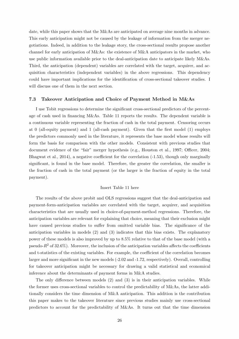
date, while this paper shows that the M&As are anticipated on average nine months in advance.

This early anticipation might not be caused by the leakage of information from the merger ne-

gotiations. Indeed, in addition to the leakage story, the cross-sectional results propose another

channel for early anticipation of M&As: the existence of M&A anticipators in the market, who

use public information available prior to the deal-anticipation date to anticipate likely M&As.

Third, the anticipation (dependent) variables are correlated with the target, acquirer, and ac-

quisition characteristics (independent variables) in the above regressions. This dependency

could have important implications for the identification of cross-sectional takeover studies. I

will discuss one of them in the next section.

7.3 Takeover Anticipation and Choice of Payment Method in M&As

I use Tobit regressions to determine the significant cross-sectional predictors of the percent-

age of cash used in financing M&As. Table 11 reports the results. The dependent variable is

a continuous variable representing the fraction of cash in the total payment. Censoring occurs

at 0 (all-equity payment) and 1 (all-cash payment). Given that the first model (1) employs

the predictors commonly used in the literature, it represents the base model whose results will

form the basis for comparison with the other models. Consistent with previous studies that

document evidence of the “fair” merger hypothesis (e.g., Houston et al., 1997; Officer, 2004;

Bhagwat et al., 2014), a negative coefficient for the correlation (-1.53), though only marginally

significant, is found in the base model. Therefore, the greater the correlation, the smaller is

the fraction of cash in the total payment (or the larger is the fraction of equity in the total

payment).

Insert Table 11 here

The results of the above probit and OLS regressions suggest that the deal-anticipation and

payment-form-anticipation variables are correlated with the target, acquirer, and acquisition

characteristics that are usually used in choice-of-payment-method regressions. Therefore, the

anticipation variables are relevant for explaining that choice, meaning that their exclusion might

have caused previous studies to suffer from omitted variable bias. The significance of the

anticipation variables in models (2) and (3) indicates that this bias exists. The explanatory

power of these models is also improved by up to 8.5% relative to that of the base model (with a

pseudo-R2 of 32.6%). Moreover, the inclusion of the anticipation variables affects the coefficients

and t-statistics of the existing variables. For example, the coefficient of the correlation becomes

larger and more significant in the new models (-2.02 and -1.72, respectively). Overall, controlling

for takeover anticipation might be necessary for drawing a valid statistical and economical

inference about the determinants of payment forms in M&A studies.

The only difference between models (2) and (3) is in their anticipation variables. While

the former uses cross-sectional variables to control the predictability of M&As, the latter addi-

tionally considers the time dimension of M&A anticipation. This addition is the contribution

this paper makes to the takeover literature since previous studies mainly use cross-sectional

predictors to account for the predictability of M&As. It turns out that the time dimension

26

is worth controlling as it provides further explanation of the payment-form choice (with the

highest pseudo-R2 between the first three models 41.1%). For example, the target firms’ cash

holdings become negatively significant for the first time in model (3). Thus, the higher the

cash holdings of the target, the less cash the acquirer will use to finance the bid. This result

suggests that target shareholders with relatively high cash reserves do not have their rights in

the acquirer firm diluted by all-cash bids, because, for example, the reserves can be used for

financing profitable projects (which has a lower cost of capital than that of external financing).

The results of previous studies might be subject to the measurement error in the first and

the second-order moments. They are often estimated over a “pre-run-up” period, e.g., over 200

trading days ending 40 days prior to the announcement (e.g., Houston and Ryngaert, 1997;

Officer, 2004). However, the results in this paper imply that early deal and payment-form

anticipation significantly shifts the second-order moments.15 The pre-announcement target and

acquirer variances are underestimated compared with those from the pre-anticipation period.

Similarly, the covariance and correlation are underestimated in cash offers and overestimated

in equity offers. The moments hence need to be estimated from the pre-anticipation segment,

a period in which the takeovers are totally unexpected. Given that anticipation might affect

other cross-sectional characteristics as well, models (4) to (6) are estimated using data from the

pre-anticipation period.

The results of these new regressions confirm the adverse effects of measurement errors on

the coefficients of the payment-method regressions. As expected, the most influential effects

are observed in the coefficients of the moments. Namely, the coefficient of the average return

of the target firms becomes significant, that of the target volatility is attenuated, and that of

the return correlation is no longer significant in all three new models. There is a significantly

positive relation between the pre-anticipation average returns of the target firms and the fraction

of cash in the bid payment. This result indicates that the acquirer expects there to be valuable

growth opportunities in the target firms with higher returns, and includes more cash in the

payment so as to dilute the future rights of the target shareholders with respect to the cash

flows. Moreover, and more importantly, the insignificance of the return correlation implies that

the relatedness of the merging firms is not a determinant of the payment form in M&As. This

result is contrary to the significant findings of previous studies, and suggests that their findings

might be affected by using the estimates from the pre-run-up period. Overall, model (6) is

the best of the six alternative models since it not only has the highest explanatory power in

predicting the choice of payment method, but is also free from the endogeneity issues caused

by omitted anticipation variables and measurement errors.

15Irani (2015) reports that the abnormal returns to the target and acquirer shareholders start to show apositive trend after the deal-anticipation date, suggesting that the pre-run-up measures of average returns areoverestimated as well. See the descriptive statistics in the internet appendix, Table C.2, which presents the twosets of measurements.

27

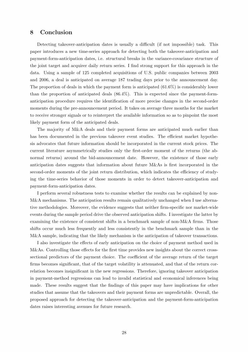
8 Conclusion

Detecting takeover-anticipation dates is usually a difficult (if not impossible) task. This

paper introduces a new time-series approach for detecting both the takeover-anticipation and

payment-form-anticipation dates, i.e. structural breaks in the variance-covariance structure of

the joint target and acquirer daily return series. I find strong support for this approach in the

data. Using a sample of 125 completed acquisitions of U.S. public companies between 2003

and 2006, a deal is anticipated on average 187 trading days prior to the announcement day.

The proportion of deals in which the payment form is anticipated (61.6%) is considerably lower

than the proportion of anticipated deals (86.4%). This is expected since the payment-form-

anticipation procedure requires the identification of more precise changes in the second-order

moments during the pre-announcement period. It takes on average three months for the market

to receive stronger signals or to reinterpret the available information so as to pinpoint the most

likely payment form of the anticipated deals.

The majority of M&A deals and their payment forms are anticipated much earlier than

has been documented in the previous takeover event studies. The efficient market hypothe-

sis advocates that future information should be incorporated in the current stock prices. The

current literature asymmetrically studies only the first-order moment of the returns (the ab-

normal returns) around the bid-announcement date. However, the existence of those early

anticipation dates suggests that information about future M&As is first incorporated in the

second-order moments of the joint return distribution, which indicates the efficiency of study-

ing the time-series behavior of those moments in order to detect takeover-anticipation and

payment-form-anticipation dates.

I perform several robustness tests to examine whether the results can be explained by non-

M&A mechanisms. The anticipation results remain qualitatively unchanged when I use alterna-

tive methodologies. Moreover, the evidence suggests that neither firm-specific nor market-wide

events during the sample period drive the observed anticipation shifts. I investigate the latter by

examining the existence of consistent shifts in a benchmark sample of non-M&A firms. Those

shifts occur much less frequently and less consistently in the benchmark sample than in the

M&A sample, indicating that the likely mechanism is the anticipation of takeover transactions.

I also investigate the effects of early anticipation on the choice of payment method used in

M&As. Controlling those effects for the first time provides new insights about the correct cross-

sectional predictors of the payment choice. The coefficient of the average return of the target

firms becomes significant, that of the target volatility is attenuated, and that of the return cor-

relation becomes insignificant in the new regressions. Therefore, ignoring takeover anticipation

in payment-method regressions can lead to invalid statistical and economical inferences being

made. These results suggest that the findings of this paper may have implications for other

studies that assume that the takeovers and their payment forms are unpredictable. Overall, the

proposed approach for detecting the takeover-anticipation and the payment-form-anticipation

dates raises interesting avenues for future research.

28

References

• Aggarwal, R.K. and M.H. Baxamusa, 2013, Unrelated acquisitions, Working Paper, http://papers.ssrn.com/sol3/papers.cfm?abstract_id=2023578 (Accessed January 12, 2015).• Ahern, K. and D. Sosyura, 2014, Who writes the news? Corporate press releases during

merger negotiations, The Journal of Finance 69, 241–291• Amihud, Y., B. Lev and N.G. Travlos, 1990, Corporate control and the choice of invest-

ment financing: the case of corporate acquisitions, The Journal of Finance 45, 603-616.• Aue, A., S. Hormann, L. Horvath and M. Reimherr, 2009, Break Detection in the Covari-

ance Structure of Multivariate Time Series Models, Annals of Statistics 37, 4046-4087.• Bai, J. and P. Perron, 1998, Estimating and testing linear models with multiple structural

changes, Econometrica 66, 47-78.• , 2003, Computation and analysis of multiple structural changes, Journal of

Applied Econometrics 18, 1-22.• , 2006, Multiple Structural Change Models: A Simulation Analysis, in Econo-

metric Theory and Practice: Frontiers of Analysis and Applied Research, D. Corbea, S.Durlauf and B.E. Hansen (eds.), Cambridge University Press, 212-237.• Berkes, I., L. Horvath, P. Kokoszka, and Q. Shao, 2005, Almost sure convergence of the

Bartlett estimator, Periodica Mathematica Hungarica 51, 11–25.• Betton, S., B.E. Eckbo, R. Thompson and K.S. Thorburn, 2014, Merger Negotiations

with Stock Market Feedback, The Journal of Finance 69, 1705–1745.• Betton, S., B.E. Eckbo and K.S. Thorburn, 2008, Corporate takeovers. In: B.E. Eckbo

(Ed.), Handbook of Corporate Finance, vol. 2. Elsevier, 291–430.• Bhagat, S., J.A. Brickley and U. Loewenstein, 1987, The pricing effects of interfirm cash

tender offers, The Journal of Finance 42, 965–986.• Bhagwat, V. and A.D. Robert, 2014, Asymmetric Interim Risk and Deal Terms in Corpo-

rate Mergers and Acquisitions, Working Paper, http://papers.ssrn.com/sol3/papers.cfm?abstract_id=1961846 (Accessed October 20, 2014).• Bharath, S.T., and G. Wu, 2006, Long-run volatility and risk around mergers and acqui-

sitions, University of Michigan, Working Paper, http://www.bauer.uh.edu/wu/Papers/Mergervol.pdf (Accessed March 1, 2013).• Bradley, M., A. Desai and E.H. Kim, 1988, Synergistic gains from corporate acquisitions

and their division between the stockholders of target and acquiring firms, Journal ofFinancial Economics 21, 3–40.• Brown, M.B. and A.B. Forsythe, 1974, Robust Tests for the Equality of Variances, Journal

of the American Statistical Association 69, 364-367.• Brown, K.C. and M.V. Raymond, 1986, Risk Arbitrage and the Prediction of Successful

Corporate Takeovers, Financial Management 15, 54-63.• Chatterjee, S. and M. Lubatkin, 1990, Corporate Mergers, Stockholder Diversification,

and Changes in Systematic Risk, Strategic Management Journal 11, 255-268.• Cornett, M.M., B. Tanyeri and H. Tehranian, 2011, The effect of merger anticipation on

bidder and target firm announcement period returns, Journal of Corporate Finance 17,595-611.• Edmans, A., I. Goldstein and W. Jiang, 2012, The Real Effects of Financial Markets: The

Impact of Prices on Takeovers, The Journal of Finance 67, 933–971.• Faccio, M. and R. Masulis, 2005, The choice of payment method in european mergers and

acquisitions, The Journal of Finance 60, 1345–1388.• Gelman, S. and B. Wilfling, 2009, Markov-switching in target stocks during takeover bids,

Journal of Empirical Finance 16, 745-758.• Geppert, G. and D.R. Kamerschen, 2008, The effect of mergers on implied volatility of

29

equity options, International Review of Financial Analysis 17, 330-344.• Groß-Klußmann, A. and N. Hautsch, 2011, When machines read the news: Using auto-

mated text analysis to quantify high frequency news-implied market reactions, Journal ofEmpirical Finance 18, 321-340.• Hamada, R.S., 1972, The effect of the firm’s capital structure on the systematic risk of

common stocks, The Journal of Finance 27, 435-45.• Harford, J., 2005, What drives merger waves?, Journal of Financial Economics 77, 529-

560.• Hasbrouck, J., 1985, The characteristics of takeover targets q and other measures, Journal

of Banking and Finance 9, 351–362.• Heckman, J.J., 1979, Sample Selection Bias as a Specification Error, Econometrica 47,

153-161.• Hutson, E. and C. Kearney, 2001, Volatility in stocks subject to takeover bids: Australian

evidence using daily data, Journal of Empirical Finance 8, 273–296.• , 2005, Stock price interaction between target and bidder stocks during takeover

bids, Research in International Business and Finance 19, 1–26.• Houston, J. and M.D. Ryngaert, 1997, Equity issuance and adverse selection: A direct

test using conditional stock offers, The Journal of Finance 52, 197–219.• Irani, M., 2015, Takeover Anticipation and Abnormal Returns, Working paper, http:

//papers.ssrn.com/sol3/papers.cfm?abstract_id=2614660.• Jayaraman, N., G. Mandelker and K. Shastri, 1991, Market anticipation of merger activ-

ities: An empirical test, Managerial and Decision Economics 12, 439-448.• Jennrich, R.I., 1970, An Asymptotic χ2 Test for the Equality of Two Correlation Matrices,

Journal of the American Statistical Association 65, 904-912.• Jensen, M.C. and R. Ruback, 1983, The Market for Corporate Control: The Scientific

Evidence, Journal of Financial Economics 11, 5-50.• Langetieg, T.C., R.S. Haugen and D.W. Wischern, 1980, Merger and stockholder risk,

Journal of Financial and Quantitative Analysis 15, 689-710.• Laughran, T. and A.M. Vijh, 1997, Do long-term shareholders benefit from corporate

acquisitions, The Journal of Finance 52, 1765-90.• Levene, H., 1960, Robust tests for equality of variances, in I. Olkin, ed., Contributions to

Probability and Statistics, P. Alto, Calif.: Stanford University Press, 278-92.• Li, K. and N. Prabhala, 2007, Self-selection models in corporate finance, In B.E. Eckbo

(ed.), Handbook of Corporate Finance: Empirical Corporate Finance, Volume 1 (Hand-books in Finance Series, Elsevier/North-Holland), 37-86.• Lim, T.S. and W.Y. Loh, 1996, A comparison of tests of equality of variances, Computa-

tional Statistical and Data Analysis 22, 287-301.• Martin, K.J., 1996, The method of payment in corporate acquisitions, investment oppor-

tunities, and management ownership, The Journal of Finance 51, 1227-1246.• Martynova, M. and L. Renneboog, 2008, A century of corporate takeovers: What have we

learned and where do we stand? Journal of Banking and Finance 32, 2148–2177.• Meulbroek, L.K., 1992, An empirical analysis of illegal insider trading, The Journal of

Finance 47, 1661–1699.• Mitchell, M.L. and J.H. Mulherin, 1996, The impact of industry shocks on takeover and

restructuring activity, Journal of Financial Economics 41, 193-229.• Newey, W.K. and K.D. West, 1994, Automatic Lag Selection in Covariance Matrix Esti-

mation, Review of Economic Studies 61, 631-53.• Officer, M., 2004, Collars and renegotiation in mergers and acquisitions, The Journal of

Finance 59, 2719–2743.• Rhodes-Kropf, M., D. Robinson and S. Viswanathan, 2005, Valuation waves and merger

activity: The empirical evidence, Journal of Financial Economics 77, 561–603.

30

• Rhodes-Kropf, M. and S. Viswanathan, 2004, Market valuation and merger waves, TheJournal of Finance 59, 2685–2718.• Rodrigues, P.M.M. and A. Rubia, 2007, On the Finite Sample Size Distortions in Non-

parametric Testing for Variance Constancy, Fundacion de Cajas de Ahorros, WorkingPaper Series N247/2007• Samuelson, W. and L. Rosenthal, 1986, Price Movements as Indicators of Tender Offer

Success, The Journal of Finance 41, 481-499.• Schwarz, G., 1978, Estimating the dimension of a model, Annals of Statistics 6, 461–464.• Schwert, G.W., 1996, Markup pricing in mergers and acquisitions, Journal of Financial

Economics 41, 153-192.• Smith, R. and J. Kim, 1994, The combined effects of free cash flow and financial slack on

bidder and target stock returns, The Journal of Business 67, 281-310.• Subramanian, A., 2004, Option pricing on stocks in mergers and acquisitions, The Journal

of Finance 59, 795–829.• Travlos, N., 1987, Corporate takeover bids, methods of payment, and bidding firms’ stock

returns, The Journal of Finance 42, 943–963.• Welch, B.L., 1947, The generalization of ’Student’s’ problem when several different pop-

ulation variances are involved, Biometrika 34, 28–35.• Wilcoxon, F., 1945, Individual comparisons by ranking methods, Biometrics 1, 80–83.

31

  49  

Figure 1 Distribution of Total Break Dates in the Variance-Covariance Structure and Box Plot of Anticipation Break Dates

Panel A of this Figure illustrates the distribution of total break dates in the variance-covariance structure (VCS) of daily acquirer and target return series relative to the announcement day (Day 0). Panel B shows the box plot of the distribution of Deal and Payment-Form anticipation break dates across payment subsamples relative to Day 0. The sample consists of 125 completed acquisitions and splits to 54 Cash, 33 Equity and 38 Mixed payment bids. The pre-announcement period is from Day-379 to Day-1 relative to the first bid announcement. The post-announcement period is from the day of first bid announcement through delisting of target shares. Each of 125 daily acquirer and target return series is sequentially adjusted for outliers, breaks in the mean, and non-zero mean (see explanation in the ( of Table 2). Aue et al. (2009) test detects the number and location of significant shifts in the VCS of each 125 bivariate return series. See the Anticipation Hypotheses (Section 3) how a break in the VCS of a deal during the pre-announcement period is recognized as Deal-Anticipation and Payment-Form-Anticipation dates. The distant and close hinges of the box plot relative to Day 0 corresponds to the 1st and 3rd quartile of anticipation dates, respectively. Moreover, the line inside the box plot presents the median of anticipation dates.

05

1015

2025

Perc

ent

-400 -300 -200 -100 0 100

Day Relative to Announcement ( Day 0 )

Panel A : Distribution of Break Dates

-400 -300 -200 -100 0Day Relative to Announcement ( Day 0 )

Mix

Equity

Cash

Panel B: Box Plot of Anticipation Break Dates

Deal-Anticipation Payment-Anticipation

Figure 1Distribution of Break and Anticipation DatesPanel A of this figure illustrates the distribution of a total of 235 break dates in the variance-covariance

structure of daily acquirer and target return series relative to the announcement date (Day 0). Panel B

shows the box plot of the distribution of deal-anticipation and payment-form-anticipation dates across

payment subsamples. Each of the 125 daily acquirer and target return series is sequentially adjusted for

outliers, breaks in the mean, and non-zero mean (see explanation in the caption of Table 4). Aue et al.’s

(2009) test detects the number and location of significant shifts in the variance-covariance structure of

each bivariate return series. See the Anticipation Hypotheses (Section 3) on how a break in the variance-

covariance structure of a deal during the pre-announcement period is recognized as the deal-anticipation

and/or the payment-form-anticipation date. The distant and close hinges of the box plot relative to Day

0 correspond to the first and the third quartiles of the anticipation dates, respectively. The line inside

the box plot represents the median of the anticipation dates.

32

   

37  

Figure 2 Shifts in Second-Order Moments of Daily Acquirer And Target Average Returns

This figure illustrates significant shifts in the second-order moments of daily acquirer and target average return series across payment subsamples. Caption of Table 8 provides further details.

Figure 2Shifts in Second-Order Moments of Daily Acquirer and Target Average ReturnsThis figure illustrates significant shifts in the second-order moments of the daily acquirer and target

average return series across payment subsamples. The caption for Table 8 provides further details.

33

   

38  

Figure 3 Average Probability of Takeover

 This figure illustrates the average probability of merging for the target and acquirer firms around the deal-anticipation (Panel A) and the bid announcement (Panel B) dates. The takeover probability at each event day

(Xt) for each firm is based on Eq. (2) in Samuelson and Rosenthal (1986): Xt =Pt −PFPT −PF

, where Pt is the stock

price of a firm at day t. The "fallback" price (PF) is its average stock price over a 20 days interval, starting 21 days prior and ending 1 day prior to the deal-anticipation date. The tender price (PT) is its stock price at the consummation date of the deal. The probability measure needs to remain in the [0,1] interval, so

Xt =Min Max Pt −PFPT −PF

"

#$

%

&', 0

(

)*

+

,-,1

./0

10

230

40. Only firms are considered in which the tender price (PT) was at least 15%

higher than the "fallback" price (PF). The initial sample considers only 108 anticipated deals while conditioning on this characteristic leads to a final sample of 84 target and 70 acquirer firms. To exclude the bid offer effects, the time series of daily takeover probability for each firm in Panel A starts 21 days prior to its deal-anticipation date and ends a day before its public announcement day.

Figure 3Average Probability of TakeoverThis figure illustrates the average probability of merging for the target and acquirer firms around the

deal-anticipation (Panel A) and the bid-announcement (Panel B) dates. The takeover probability on

each event day (Xt) for each firm is based on Eq. (2) in Samuelson and Rosenthal (1986): Xt =

(Pt−PF )/(PT−PF ), where Pt is the stock price of a firm on day t. The ”fallback” price (PF ) is its average

stock price over a 20-day interval, starting 21 days prior to and ending 1 day prior to the deal-anticipation

date. The tender price (PT ) is the stock price on the deal-consummation date. The probability measure

needs to remain in the [0, 1] interval, so Xt = Min {Max [(Pt − PF )/(PT − PF ), 0] , 1}. Firms are only

considered if the tender price (PT ) was at least 15% higher than the ”fallback” price (PF ). The initial

sample considers the 108 anticipated deals, while conditioning on this characteristic leads to a final

sample of 84 target and 70 acquirer firms. To exclude the bid-offer effects, the time series of daily

takeover probabilities for each firm in Panel A starts 21 days prior to its deal-anticipation date and ends

a day before its public announcement date.

34

   

39  

Figure 4 Synergistic Gains to the Anticipators of Target and Acquirer Firms

  Using the S&P 500 index, the market model estimates the abnormal return (AR) at day t around the deal anticipation date (Day 0) for each target and acquirer firm. The float estimation window, which contains returns from the pre-anticipation segment of each anticipated deals, estimates the parameters of the model. The subsample of 108 anticipated deals is used to construct the cumulative average abnormal returns (CAARs). To exclude the announcement effect on the estimates of CAARs, the time series of daily returns for each firm ends a day before its public announcement day. See Irani (2014) for further explanation about the estimation approach.

 

 

 

 

 

 

 

 

 

Figure 4Returns around Anticipation DateThis figure illustrates the returns to the target and acquirer shareholders around the deal-anticipation

dates. Using the S&P 500 index, the market model estimates the abnormal return (AR) on day t around

the deal-anticipation date (Day 0) for each target and acquirer firm. The float estimation window, which

contains returns from the pre-anticipation segment of each anticipated deal, estimates the parameters of

the model. The subsample of 108 anticipated deals is used to construct the cumulative average abnormal

returns (CAARs). To exclude the announcement effect on the estimates of the CAARs, the time series of

daily returns for each firm ends a day before its public announcement date. See Irani (2015) for further

explanation of the estimation approach.

35

Table 1Expected Shifts for Detecting the Deal-Anticipation and Payment-Form-Anticipation Dates

This table presents how a deal and its payment form can be anticipated based on expected shift(s) in

the second-order moments. Panels A, B, and C show possible outcomes in which the test (of Aue et al.,

2009) detects no, one, and two breaks in the variance-covariance structure of a bivariate target-acquirer

return series during the pre-announcement period (-379, -1), respectively. When there are two breaks,

K1 is detected before K2, i.e. -379 <K1 <K2 <0. +, - and +/- denote a significant positive shift, a

significant negative shift, and a significant shift of either sign in the second-order moments, respectively.

A significant negative shift (-) in the covariance or correlation is a shift towards zero.

Possible Target Acquirer Target Acquirer

Outcome Variance Variance Covariance Correlation Variance Variance Covariance Correlation Deal Cash Equity

1 Unanticipated

2 + +/- +/- +/- Unanticipated

3 - +/- + + K 1 K 1

4 - +/- - - K 1 K 1

5 + +/- +/- +/- + +/- +/- +/- Unanticipated

6 - +/- +/- +/- + +/- +/- +/- Unanticipated

7 + +/- +/- +/- - +/- + + K 2 K 2

8 + +/- +/- +/- - +/- - - K 2 K 2

9 - +/- + + - +/- + + K 1 K 1

10 - +/- - - - +/- - - K 1 K 1

11 - +/- + + - +/- - - K 1 K 2

12 - +/- - - - +/- + + K 1 K 2

Panel B: One Break (K 1 )

Unanticipated

Panel C: Two Breaks (K 1 and K 2 )

Unanticipated

Unanticipated

Shifts after First Break (K 1 ) Shifts after Second Break (K 2 ) Anticipation Date

Payment-Form

Panel A: No Break

Unanticipated

36

Table 2Sample Selection

This table describes the sample selection process. All bids are completed “mergers” and “acquisitions”

between U.S. publicly listed target and acquirer firms between June 2003 and June 2006, retrieved from

the Bureau Van Dijk Zephyr database. Adjusted daily closing prices of stocks are taken from Thomson

Financial DataStream.

Selection Criteria Source

All completed mergers and acquisitions between U.S. publicly listed firms

during the period 6/2003 to 6/2006 Zephyr 1647

Bid offer is for 100% of the target shares Zephyr 1120 527

Payment-form is Cash, Equity, or Mixed Zephyr 78 449

Completion date is between 19 and 253 days Zephyr 37 412

Deal value > $50 million Zephyr 78 334

Both acquirer and target firm are not banks Zephyr 108 226

One bid record for any acquirer in this sample period Zephyr 46 180

Targets stock price on Day -42 > 2$ DataStream 13 167

At least 120 daily stock prices is available in the pre-announcement period DataStream 42 125

Final Sample 125

Number of

Exclusions

Sample

Size

37

Table 3Summary Statistics of Sample Second-Order Moments

This table presents descriptive statistics for the sample second-order moments of the acquirer and target

return series during the pre- and post-announcement periods. The sample consists of 125 completed ac-

quisitions and splits into 54 cash, 33 equity, and 38 mixed-payment bids. The pre-announcement period

is from Day -379 to Day -1 relative to the first bid-announcement date. The post-announcement period

is from the announcement date through to the delisting date of the target shares. All volatility and co-

variance estimates are annualized over 252 trading days. The matched-pairs t-test (the Wilcoxon (1945)

matched-pairs signed-rank test) examines the difference between the cross-sectional averages (medians)

of the pre- and post-announcement moments. The one-way ANOVA model tests the equality-of-means

across payment subsamples. All the above tests are two-tailed tests. ***, ** and * denote statistical

significant at the 1%, 5% and 10% levels, respectively.

F-Value

Period Mean Std. Dev. 25th 50th 75th t -Stat. Sign-Rank Z-Stat. Cash Equity Mixed ANOVA

Pre-Ann. 0.483 0.190 0.335 0.463 0.608 0.467 0.512 0.482 0.60

Post-Ann. 0.270 0.131 0.180 0.245 0.331 -17.89*** -9.66*** 0.214 0.361 0.272 16.28***

Pre-Ann. 0.384 0.182 0.263 0.331 0.461 0.336 0.441 0.405 3.95**

Post-Ann. 0.318 0.139 0.215 0.295 0.379 -7.28*** -6.79*** 0.284 0.357 0.331 3.13**

Pre-Ann. 0.047 0.056 0.013 0.029 0.061 0.029 0.066 0.056 5.72***

Post-Ann. 0.045 0.086 0.001 0.016 0.077 -0.23 -2.34** 0.0003 0.110 0.054 22.93***

Pre-Ann. 0.245 0.191 0.092 0.213 0.352 0.170 0.305 0.301 8.32***

Post-Ann. 0.340 0.400 0.025 0.250 0.754 3.08*** 2.86*** 0.026 0.685 0.487 62.53***

Acquirer-Target Correlation

Mean

Target Volatility

Acquirer Volatility

Acquirer-Target Covariance

Percentile Difference (Post - Pre)

38

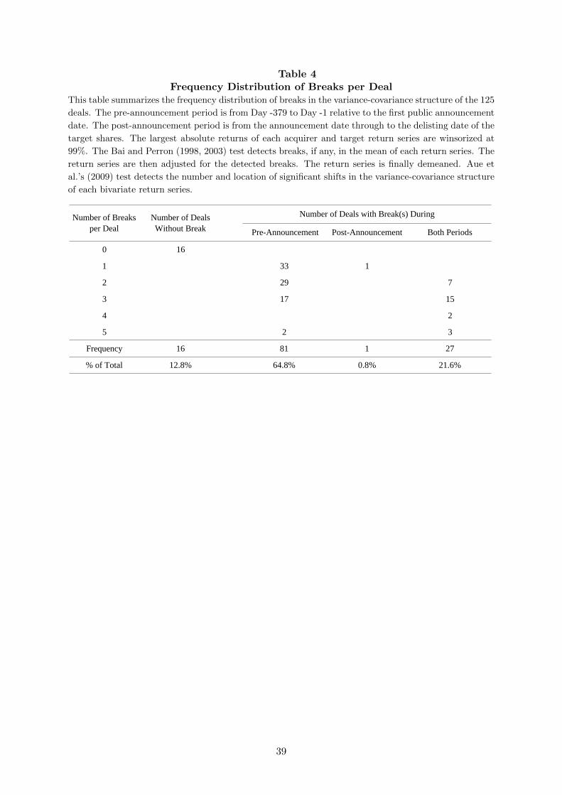
Table 4Frequency Distribution of Breaks per Deal

This table summarizes the frequency distribution of breaks in the variance-covariance structure of the 125

deals. The pre-announcement period is from Day -379 to Day -1 relative to the first public announcement

date. The post-announcement period is from the announcement date through to the delisting date of the

target shares. The largest absolute returns of each acquirer and target return series are winsorized at

99%. The Bai and Perron (1998, 2003) test detects breaks, if any, in the mean of each return series. The

return series are then adjusted for the detected breaks. The return series is finally demeaned. Aue et

al.’s (2009) test detects the number and location of significant shifts in the variance-covariance structure

of each bivariate return series.

Pre-Announcement Post-Announcement Both Periods

0 16

1 33 1

2 29 7

3 17 15

4 2

5 2 3

Frequency 16 81 1 27

% of Total 12.8% 64.8% 0.8% 21.6%

Number of Breaks

per Deal

Number of Deals

Without Break

Number of Deals with Break(s) During

39

Table 5Summarized Results of Deal-Anticipation and Payment-Form-Anticipation DatesThis table presents the descriptive statistics of the deal-anticipation and payment-form-anticipation dates

relative to the announcement date (Day 0). The total sample consists of 125 acquisitions and splits into

54 cash, 33 equity and 38 mixed-payment bids. Each of the 125 daily acquirer and target return series is

sequentially adjusted for outliers, breaks in the mean, and non-zero mean (see explanation in the caption

of Table 4). Aue et al.’s (2009) test detects the number and location of significant shifts in the variance-

covariance structure of each bivariate return series. See the Anticipation Hypotheses (Section 3) on how

a break in the variance-covariance structure of a deal during the pre-announcement period is recognized

as a deal-anticipation and/or payment-form-anticipation date. Welch’s (1947) unpaired unequal variance

option of the t-test examines the difference between average deal- and payment-form-anticipation dates.

The one-way ANOVA tests the equality-of-average-anticipation-dates across payment subsamples. All

the above tests are two-tailed tests. ***, ** and * denote statistical significant at the 1%, 5% and 10%

levels, respectively.

Number Dif. (Deal - Payment)

(Sub)Sample of Deals Mean Std. Dev. 25th 50th 75th t -Stat.

Total 108 -186.6 87.3 -253 -190 -133 -4.49*** 0.05

Cash 46 -189.2 84.0 -253 -198 -130 -1.41

Equity 30 -186.2 78.4 -249 -186 -139 -4.29***

Mixed 32 -183.2 101.4 -257 -204 -93 -3.07**

Total 77 -123.1 99.8 -210 -106 -25 6.11***

Cash 37 -161.8 91.4 -240 -171 -92

Equity 21 -83.1 88.7 -135 -64 -3

Mixed 19 -91.8 103.3 -193 -52 -1

Percentile F-Value

ANOVA

Deal-Anticipation Breaks

Payment-Form Anticipation Breaks

40

Table 6Summary Statistics of Second-Order Moments around Deal-Anticipation Dates

This table summarizes the descriptive statistics of the sample second-order moments of the acquirer and

target return series during the pre- and post-anticipation segments. The total sample of anticipated

deals contains 108 deals and splits into 46 cash, 30 equity and 32 mixed-payment bids. The sample

unconditional moments are computed across these segments in the usual way. All volatility and covari-

ance estimates are annualized over 252 trading days. The matched-pairs t-test (the Wilcoxon (1945)

matched-pairs signed-rank test) examines the difference between the cross-sectional averages (medians)

of the post- and pre-anticipation moments. The one-way ANOVA tests the equality-of-means across

payment subsamples. All the above tests are two-tailed tests. ***, ** and * denote statistical significant

at the 1%, 5% and 10% levels, respectively.

(Sub)sample Period Mean Std. Dev. 25th 50th 75th t -Stat. Sign-Rank Z-Stat.

Total Pre-Ant. 0.552 0.236 0.381 0.509 0.685 0.11

Post-Ant. 0.443 0.225 0.294 0.404 0.557 -6.53*** -6.58*** 1.78

Cash Pre-Ant. 0.544 0.229 0.378 0.528 0.667

Post-Ant. 0.419 0.177 0.287 0.408 0.546 -5.97*** -5.03***

Equity Pre-Ant. 0.548 0.241 0.409 0.509 0.691

Post-Ant. 0.509 0.302 0.339 0.421 0.609 -0.90 -1.57

Mixed Pre-Ant. 0.569 0.247 0.371 0.501 0.751

Post-Ant. 0.416 0.197 0.259 0.359 0.569 -6.89*** -4.69***

Total Pre-Ant. 0.443 0.233 0.276 0.368 0.557 2.74*

Post-Ant. 0.374 0.232 0.226 0.336 0.434 -5.02*** -5.59*** 2.91**

Cash Pre-Ant. 0.384 0.172 0.274 0.344 0.467

Post-Ant. 0.332 0.180 0.223 0.296 0.386 -2.84*** -3.08***

Equity Pre-Ant. 0.494 0.281 0.312 0.439 0.618

Post-Ant. 0.458 0.340 0.259 0.366 0.473 -1.15 -2.23**

Mixed Pre-Ant. 0.481 0.247 0.278 0.430 0.635

Post-Ant. 0.354 0.145 0.229 0.330 0.443 -5.58*** -4.45***

Total Pre-Ant. 0.063 0.084 0.012 0.033 0.092 1.59

Post-Ant. 0.050 0.101 0.008 0.025 0.065 -1.35 -3.39*** 4.56**

Cash Pre-Ant. 0.047 0.064 0.009 0.028 0.042

Post-Ant. 0.024 0.038 0.002 0.014 0.031 -2.81*** -2.94***

Equity Pre-Ant. 0.080 0.094 0.007 0.056 0.116

Post-Ant. 0.093 0.173 0.019 0.051 0.092 0.47 -0.73

Mixed Pre-Ant. 0.071 0.098 0.023 0.047 0.103

Post-Ant. 0.047 0.047 0.014 0.036 0.067 -1.86* -1.98**

Total Pre-Ant. 0.248 0.211 0.103 0.225 0.375 2.84*

Post-Ant. 0.252 0.235 0.067 0.206 0.418 0.23 -0.12 8.31***

Cash Pre-Ant. 0.195 0.154 0.058 0.171 0.315

Post-Ant. 0.152 0.160 0.043 0.152 0.250 -1.58 -1.28

Equity Pre-Ant. 0.304 0.257 0.126 0.288 0.522

Post-Ant. 0.338 0.267 0.132 0.319 0.559 0.80 0.13

Mixed Pre-Ant. 0.272 0.222 0.118 0.256 0.411

Post-Ant. 0.316 0.248 0.138 0.285 0.495 1.16 0.99

Target Volatility

Acquirer Volatility

Acquirer-Target Covariance

Acquirer-Target Correlation

Percentile Difference (Post - Pre) F-Value

ANOVA

41

Table 7Summary Statistics of Second-Order Moments around Payment-Form Anticipation Date

This table summarizes the descriptive statistics of the sample second-order moments of the acquirer and

target return series during the pre- and post-payment-form-anticipation segments. The total sample

of payment-form-anticipated deals contains 77 deals and splits into 37 cash, 21 equity and 19 mixed-

payment bids. The sample unconditional moments are computed across these segments in the usual way.

All volatility and covariance estimates are annualized over 252 trading days. The matched-pairs t-test

(the Wilcoxon (1945) matched-pairs signed-rank test) examines the difference between the cross-sectional

averages (medians) of the post- and pre-anticipation moments. The one-way ANOVA model tests the

equality-of-means across payment subsamples. All the above tests are two-tailed tests. ***, ** and *

denote statistical significant at the 1%, 5% and 10% levels, respectively.

(Sub)sample Period Mean Std. Dev. 25th 50th 75th t -Stat. Sign-Rank Z-Stat.

Total Pre-Ant. 0.490 0.241 0.349 0.449 0.613 1.41

Post-Ant. 0.369 0.176 0.259 0.343 0.450 -6.92*** -6.12*** 2.09

Cash Pre-Ant. 0.530 0.225 0.378 0.522 0.625

Post-Ant. 0.382 0.159 0.279 0.389 0.495 -5.87*** -4.50***

Equity Pre-Ant. 0.489 0.295 0.289 0.421 0.670

Post-Ant. 0.408 0.209 0.292 0.388 0.460 -1.87* -1.83*

Mixed Pre-Ant. 0.416 0.198 0.304 0.383 0.498

Post-Ant. 0.301 0.156 0.180 0.271 0.369 -6.41*** -3.74***

Total Pre-Ant. 0.380 0.187 0.229 0.346 0.467 1.00

Post-Ant. 0.339 0.171 0.222 0.322 0.410 -3.11*** -3.39*** 2.92*

Cash Pre-Ant. 0.365 0.153 0.247 0.352 0.450

Post-Ant. 0.302 0.119 0.205 0.293 0.378 -3.68*** -3.22***

Equity Pre-Ant. 0.429 0.251 0.224 0.346 0.507

Post-Ant. 0.412 0.261 0.258 0.333 0.455 -0.53 -1.30

Mixed Pre-Ant. 0.354 0.164 0.222 0.286 0.531

Post-Ant. 0.328 0.105 0.229 0.343 0.416 -1.15 -0.81

Total Pre-Ant. 0.047 0.061 0.012 0.029 0.059 0.54

Post-Ant. 0.048 0.105 0.004 0.020 0.056 0.09 -1.03 8.67***

Cash Pre-Ant. 0.054 0.063 0.020 0.031 0.059

Post-Ant. 0.012 0.024 0.001 0.005 0.014 -5.4*** -5.05***

Equity Pre-Ant. 0.039 0.062 0.006 0.023 0.067

Post-Ant. 0.120 0.178 0.033 0.076 0.135 2.39** 4.02***

Mixed Pre-Ant. 0.041 0.058 0.012 0.025 0.054

Post-Ant. 0.038 0.030 0.017 0.031 0.056 -0.21 0.2

Total Pre-Ant. 0.255 0.199 0.125 0.239 0.393 0.63

Post-Ant. 0.322 0.323 0.060 0.201 0.641 1.91* 1.62 39.56***

Cash Pre-Ant. 0.234 0.159 0.142 0.227 0.337

Post-Ant. 0.089 0.132 0.007 0.066 0.196 -5.21*** -4.32***

Equity Pre-Ant. 0.252 0.239 0.037 0.227 0.413

Post-Ant. 0.610 0.266 0.456 0.655 0.820 9.18*** 4.02***

Mixed Pre-Ant. 0.297 0.224 0.098 0.254 0.477

Post-Ant. 0.456 0.314 0.153 0.537 0.713 2.16** 2.01**

Target Volatility

Acquirer Volatility

Acquirer-Target Covariance

Acquirer-Target Correlation

Percentile Difference (Post - Pre) F-Value

ANOVA

42

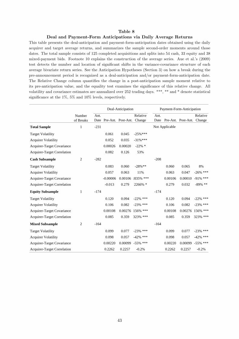
Table 8Deal and Payment-Form Anticipations via Daily Average Returns

This table presents the deal-anticipation and payment-form-anticipation dates obtained using the daily

acquirer and target average returns, and summarizes the sample second-order moments around those

dates. The total sample consists of 125 completed acquisitions and splits into 54 cash, 33 equity and 38

mixed-payment bids. Footnote 10 explains the construction of the average series. Aue et al.’s (2009)

test detects the number and location of significant shifts in the variance-covariance structure of each

average bivariate return series. See the Anticipation Hypotheses (Section 3) on how a break during the

pre-announcement period is recognized as a deal-anticipation and/or payment-form-anticipation date.

The Relative Change column quantifies the change in a post-anticipation sample moment relative to

its pre-anticipation value, and the equality test examines the significance of this relative change. All

volatility and covariance estimates are annualized over 252 trading days. ***, ** and * denote statistical

significance at the 1%, 5% and 10% levels, respectively.

Ant.

Date Pre-Ant. Post-Ant.

Relative

Change

Ant.

Date Pre-Ant. Post-Ant.

Relative

Change

Total Sample 1 -231

Target Volatility 0.061 0.045 -25%***

Acquirer Volatility 0.052 0.035 -31%***

Acquirer-Target Covariance 0.00026 0.00020 -22% *

Acquirer-Target Correlation 0.082 0.126 53%

Cash Subsample 2 -282 -208

Target Volatility 0.083 0.060 -28%** 0.060 0.065 8%

Acquirer Volatility 0.057 0.063 11% 0.063 0.047 -26% ***

Acquirer-Target Covariance -0.00006 0.00106 1835% *** 0.00106 0.00010 -91% ***

Acquirer-Target Correlation -0.013 0.279 2266% * 0.279 0.032 -89% **

Equity Subsample 1 -174 -174

Target Volatility 0.120 0.094 -22% *** 0.120 0.094 -22% ***

Acquirer Volatility 0.106 0.082 -23% *** 0.106 0.082 -23% ***

Acquirer-Target Covariance 0.00108 0.00276 156% *** 0.00108 0.00276 156% ***

Acquirer-Target Correlation 0.085 0.359 323% *** 0.085 0.359 323% ***

Mixed Subsample 2 -164 -164

Target Volatility 0.099 0.077 -23% *** 0.099 0.077 -23% ***

Acquirer Volatility 0.098 0.057 -42% *** 0.098 0.057 -42% ***

Acquirer-Target Covariance 0.00220 0.00099 -55% *** 0.00220 0.00099 -55% ***

Acquirer-Target Correlation 0.2262 0.2257 -0.2% 0.2262 0.2257 -0.2%

Number

of Breaks

Deal-Anticipation Payment-Form-Anticipation

Not Applicable

43

Table 9Probit Estimations of Deal-Anticipation and Payment-Form-Anticipation Probabilities

This table presents the parameter estimates from the probit regressions for the probability that a deal

is anticipated (columns 1 and 2), and for the probability that an offered payment form is anticipated

(columns 4 and 5). The dependent variable in columns (1) to (3) is an indicator equal to 1 if the deal is

anticipated, and 0 otherwise; and in columns (4) to (6) is an indicator equal to 1 if the payment form

is anticipated, and 0 otherwise. Models (1) to (3) consider the total sample of 125 deals while models

(4) to (6) consider the subsample of 108 anticipated deals. Columns (3) and (6) report the average

marginal effects (dP/dx ) of the models in columns (2) and (5), respectively. The numbers in parenthesis

denote the z-values, which are based on (Huber/White) heteroskedasticity-consistent standard errors

(columns 1, 2, 4, and 5) and delta-method standard errors (columns 3 and 6). The irrelevant predictors

for exclusion from the full models so as to construct the nested models are selected to minimize the

BIC (Bayesian information criterion of Schwarz, 1978) without deteriorating the predictive power of the

models (pseudo-R2). The Wald test examines the joint insignificance of those predictors, and its P-value

is reported. ***, ** and * denote statistical significance at the 1%, 5% and 10% levels, respectively. See

internet appendix Table C.1 for variable definitions.

Dependent Variable

Full Model Full Model

(1) (2) (3) (4) (5) (6)

Coeff. Coeff. (dP /dx ) Coeff. Coeff. (dP /dx )

Intercept 8.17 6.89 4.07 4.78

(2.1)** (1.83)* (1.07) (1.37)

Pre-Anticipation Return Moments

Target average stock return 1.55 1.47 0.19 0.21

(3.67)*** (3.58)*** (3.84)*** (0.7)

Acquirer average stock return 0.44 0.57 0.07 -0.55 -0.44 -0.10

(1.08) (1.67)* (1.80)* (-2.28)** (-2.27)** (-2.45)**

Target stock volatility -0.14 0.76

(-0.08) (0.72)

Acquirer stock volatility -0.65 1.72 1.68 0.39

(-0.42) (1.55) (1.89)* (1.96)**

Target-acquirer stock covariance 19.66 20.10 2.54 -3.25 -2.13 -0.49

(2.86)*** (3.00)*** (3.20)*** (-0.99) (-0.8) (-0.8)

Target-acquirer stock correlation -1.57 -1.72 -0.22 3.23 2.70 0.62

(-0.92) (-1.07) (-1.06) (1.88)* (1.84)* (1.89)*

Target Characteristics

Sales -0.33 -0.29 -0.04 -0.47 -0.33 -0.08

(-1.13) (-1.22) (-1.26) (-1.43) (-1.39) (-1.38)

Ln (Market Capitalization) -0.79 -0.67 -0.08 -0.27 -0.19 -0.04

(-2.43)** (-2.20)** (-2.43)** (-0.98) (-1.17) (-1.17)

ROE 0.95 0.93 0.12 0.13

(3.35)*** (3.84)*** (4.34)*** (0.17)

Leverage -0.63 2.41 2.16 0.50

(-0.39) (1.83)* (1.59) (1.63)

Cash holdings -4.32 -3.93 -0.50 0.19

(-3.63)*** (-3.30)*** (-3.87)*** (0.21)

Tobin's Q -0.01 -0.18 -0.15 -0.03

(-0.05) (-1.69)* (-1.7)* (-1.77)*

Deal Anticipation Payment-Form Anticipation

Nested Model Nested Model

44

Table 9 - continued

Dependent Variable

Full Model Full Model

(1) (2) (3) (4) (5) (6)

Coeff. Coeff. (dP /dx ) Coeff. Coeff. (dP /dx )

Acquirer Characteristics

Sales 0.11 0.23

(0.31) (0.67)

Ln (Market Capitalization) 0.38 0.32 0.04 0.08

(1.63) (1.72)* (1.83)* (0.42)

ROE -0.77 -0.41

(-0.66) (-0.8)

Leverage 1.79 1.81 0.23 3.07 2.74 0.63

(1.36) (1.42) (1.41) (2.55)** (2.45)** (2.39)**

Cash holdings 0.24 0.24

(0.14) (0.2)

Tobin's Q 0.42 0.37 0.05 0.18 0.15 0.03

(1.56) (2.93)*** (3.14)*** (1.26) (1.26) (1.29)

Deal Characteristics

Rumor 0.25 -0.24

(0.42) (-0.35)

Same industry -0.02 -1.13 -1.07 -0.25

(-0.04) (-3.27)*** (-3.04)*** (-3.23)***

Relative size 0.85 0.76 0.10 0.95 0.69 0.16

(1.47) (1.43) (1.48) (1.8)* (2.05)** (2.05)**

Cash offer -1.28 -1.06 -0.13 1.07 1.06 0.24

(-2.38)** (-2.46)** (-2.40)** (2.28)** (2.69)*** (2.89)***

IT industry 2.00 1.93 0.24 -0.63 -0.51 -0.12

(2.98)*** (3.39)*** (3.47)*** (-1.5) (-1.4) (-1.45)

Market Volatility 13.77 12.66 1.60 -8.38 -6.77 -1.55

(1.76)* (1.70)* (1.72)* (-1.41) (-1.64)* (-1.69)*

Announcement-year dummies Yes Yes Yes Yes Yes Yes

N(dep. Var. =1) 108 108 77 77

N(dep. Var. =0) 17 17 31 31

(P > ) of excluded predictors 0.9997 0.9886

BIC 192.05 149.33 217.88 177.59

51.21 35.94 47.78 45.73

Pseudo - R2 0.428 0.421 0.330 0.316

Nested Model Nested Model

Deal Anticipation Payment-Form Anticipation

2

2

45

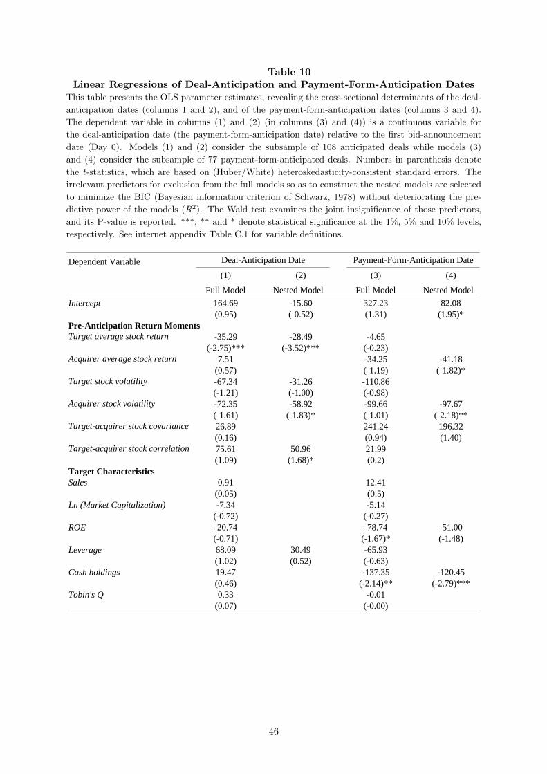
Table 10Linear Regressions of Deal-Anticipation and Payment-Form-Anticipation Dates

This table presents the OLS parameter estimates, revealing the cross-sectional determinants of the deal-

anticipation dates (columns 1 and 2), and of the payment-form-anticipation dates (columns 3 and 4).

The dependent variable in columns (1) and (2) (in columns (3) and (4)) is a continuous variable for

the deal-anticipation date (the payment-form-anticipation date) relative to the first bid-announcement

date (Day 0). Models (1) and (2) consider the subsample of 108 anticipated deals while models (3)

and (4) consider the subsample of 77 payment-form-anticipated deals. Numbers in parenthesis denote

the t-statistics, which are based on (Huber/White) heteroskedasticity-consistent standard errors. The

irrelevant predictors for exclusion from the full models so as to construct the nested models are selected

to minimize the BIC (Bayesian information criterion of Schwarz, 1978) without deteriorating the pre-

dictive power of the models (R2). The Wald test examines the joint insignificance of those predictors,

and its P-value is reported. ***, ** and * denote statistical significance at the 1%, 5% and 10% levels,

respectively. See internet appendix Table C.1 for variable definitions.

Dependent Variable

(1) (2) (3) (4)

Full Model Nested Model Full Model Nested Model

Intercept 164.69 -15.60 327.23 82.08

(0.95) (-0.52) (1.31) (1.95)*

Pre-Anticipation Return Moments

Target average stock return -35.29 -28.49 -4.65

(-2.75)*** (-3.52)*** (-0.23)

Acquirer average stock return 7.51 -34.25 -41.18

(0.57) (-1.19) (-1.82)*

Target stock volatility -67.34 -31.26 -110.86

(-1.21) (-1.00) (-0.98)

Acquirer stock volatility -72.35 -58.92 -99.66 -97.67

(-1.61) (-1.83)* (-1.01) (-2.18)**

Target-acquirer stock covariance 26.89 241.24 196.32

(0.16) (0.94) (1.40)

Target-acquirer stock correlation 75.61 50.96 21.99

(1.09) (1.68)* (0.2)

Target Characteristics

Sales 0.91 12.41

(0.05) (0.5)

Ln (Market Capitalization) -7.34 -5.14

(-0.72) (-0.27)

ROE -20.74 -78.74 -51.00

(-0.71) (-1.67)* (-1.48)

Leverage 68.09 30.49 -65.93

(1.02) (0.52) (-0.63)

Cash holdings 19.47 -137.35 -120.45

(0.46) (-2.14)** (-2.79)***

Tobin's Q 0.33 -0.01

(0.07) (-0.00)

Deal-Anticipation Date Payment-Form-Anticipation Date

46

Table 10 - continued

Dependent Variable

(1) (2) (3) (4)

Full Model Nested Model Full Model Nested Model

Acquirer Characteristics

Sales -5.24 -22.03 -12.47

(-0.39) (-1.01) (-1.28)

Ln (Market Capitalization) -0.43 -5.89

(-0.06) (-0.53)

ROE 37.02 29.05 23.81

(1.51) (1.76)* (0.58)

Leverage -98.73 -119.49 -85.63 -90.35

(-2.16)** (-3.11)*** (-1.23) (-1.79)*

Cash holdings 23.53 -8.70

(0.44) (-0.1)

Tobin's Q -0.54 4.08

(-0.08) (0.29)

Deal Characteristics

Rumor -15.77 -11.30

(-0.61) (-0.35)

Same industry -2.82 17.82

(-0.17) (0.59)

Relative size -5.62 -0.55

(-0.42) (-0.03)

Cash offer -13.63 -77.93 -66.13

(-0.63) (-2.22)** (-3.23)***

IT industry -2.77 23.01

(-0.12) (0.75)

Market Volatility -885.55 -830.00 -364.88 -550.77

(-3.71)*** (-4.69)*** (-0.71) (-1.85)*

Announcement-year dummies Yes Yes Yes Yes

Observations 108 108 77 77

(P > ) of excluded predictors 0.9881 0.983

BIC 1329.07 1260.96 1002.40 944.08

F-Value 5.17 11.27 4.90 6.44

R2 0.491 0.458 0.448 0.396

Deal-Anticipation Date Payment-Form-Anticipation Date

2

47

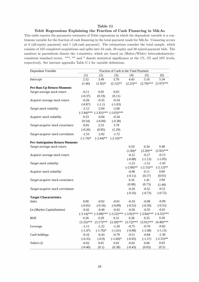
Table 11Tobit Regressions Explaining the Fraction of Cash Financing in M&As

This table reports the parameter estimates of Tobit regressions in which the dependent variable is a con-

tinuous variable for the fraction of cash financing in the total payment made for M&As. Censoring occurs

at 0 (all-equity payment) and 1 (all-cash payment). The estimations consider the total sample, which

consists of 125 completed acquisitions and splits into 54 cash, 33 equity and 38 mixed-payment bids. The

numbers in parenthesis denote the t-statistics, which are based on (Huber/White) heteroskedasticity-

consistent standard errors. ***, ** and * denote statistical significance at the 1%, 5% and 10% levels,

respectively. See internet appendix Table C.1 for variable definitions.

Dependent Variable

(1) (2) (3) (4) (5) (6)

Intercept 2.52 3.49 3.76 4.45 5.16 5.34

(1.40) (1.92)* (2.12)** (2.22)** (2.70)*** (2.97)***

Target average stock return -0.11 0.05 0.03

(-0.37) (0.19) (0.11)

Acquirer average stock return -0.26 -0.35 -0.34

(-0.87) (-1.1) (-1.03)

Target stock volatility -2.12 -2.04 -2.06

(-2.84)*** (-2.81)*** (-3.03)***

Acquirer stock volatility 0.53 -0.04 -0.34

(0.54) (-0.04) (-0.38)

Target-acquirer stock covariance -0.81 2.53 3.78

(-0.26) (0.85) (1.29)

Target-acquirer stock correlation -1.53 -2.02 -1.72

(-1.74)* (-2.44)** (-2.16)**

Target average stock return 0.29 0.34 0.48

(1.84)* (2.20)** (2.92)***

Acquirer average stock return -0.12 -0.17 -0.13

(-0.88) (-1.13) (-1.05)

Target stock volatility -1.53 -1.51 -1.43

(-2.08)** (-2.15)** (-2.12)**

Acquirer stock volatility -0.08 0.11 0.00

(-0.11) (0.17) (0.01)

Target-acquirer stock covariance 0.16 1.41 2.94

(0.08) (0.73) (1.46)

Target-acquirer stock correlation -0.26 -0.52 -0.51

(-0.35) (-0.73) (-0.75)

Target Characteristics

Sales 0.00 -0.02 -0.01 -0.10 -0.08 -0.09

(-0.02) (-0.16) (-0.09) (-0.52) (-0.50) (-0.55)

Ln (Market Capitalization) -0.42 -0.40 -0.43 -0.56 -0.55 -0.61

(-3.14)*** (-3.08)*** (-3.22)*** (-3.92)*** (-3.84)*** (-4.32)***

ROE 0.26 0.29 0.31 0.28 0.35 0.39

(3.33)*** (3.17)*** (3.39)*** (3.72)*** (3.91)*** (4.48)***

Leverage -1.11 -1.22 -1.20 -0.75 -0.76 -0.82

(-1.47) (-1.76)* (-1.61) (-0.98) (-1.08) (-1.13)

Cash holdings -0.16 -0.43 -0.79 -0.51 -0.84 -1.36

(-0.35) (-0.9) (-1.69)* (-0.95) (-1.57) (-2.55)**

Tobin's Q -0.02 0.01 0.02 -0.02 0.00 0.03

(-0.40) (0.1) (0.38) (-0.43) (0.03) (0.5)

Fraction of Cash in the Total Payment

Pre-Run-Up Return Moments

Pre-Anticipation Return Moments

48

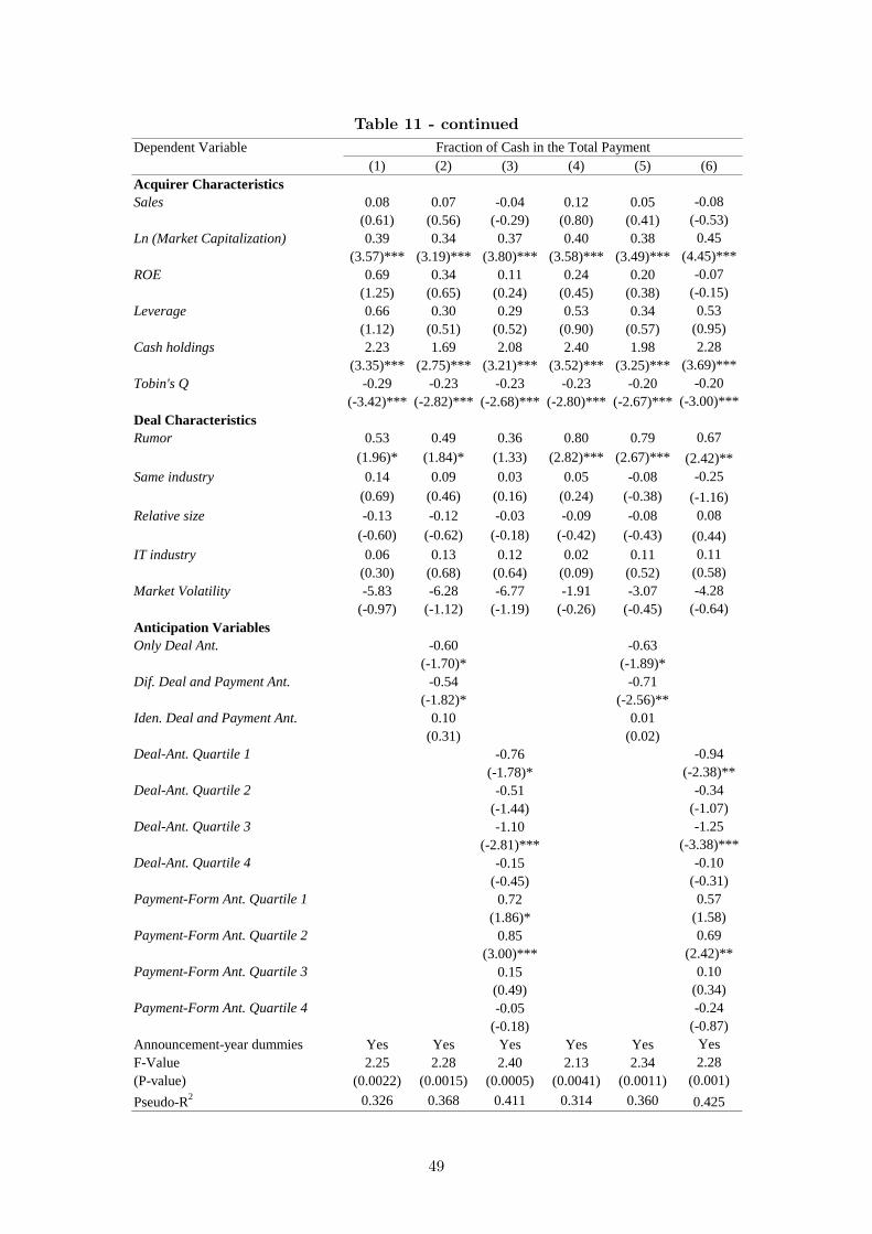
Table 11 - continued

Dependent Variable

(1) (2) (3) (4) (5) (6)

Acquirer Characteristics

Sales 0.08 0.07 -0.04 0.12 0.05 -0.08

(0.61) (0.56) (-0.29) (0.80) (0.41) (-0.53)

Ln (Market Capitalization) 0.39 0.34 0.37 0.40 0.38 0.45

(3.57)*** (3.19)*** (3.80)*** (3.58)*** (3.49)*** (4.45)***

ROE 0.69 0.34 0.11 0.24 0.20 -0.07

(1.25) (0.65) (0.24) (0.45) (0.38) (-0.15)

Leverage 0.66 0.30 0.29 0.53 0.34 0.53

(1.12) (0.51) (0.52) (0.90) (0.57) (0.95)

Cash holdings 2.23 1.69 2.08 2.40 1.98 2.28

(3.35)*** (2.75)*** (3.21)*** (3.52)*** (3.25)*** (3.69)***

Tobin's Q -0.29 -0.23 -0.23 -0.23 -0.20 -0.20

(-3.42)*** (-2.82)*** (-2.68)*** (-2.80)*** (-2.67)*** (-3.00)***

Deal Characteristics

Rumor 0.53 0.49 0.36 0.80 0.79 0.67

(1.96)* (1.84)* (1.33) (2.82)*** (2.67)*** (2.42)**

Same industry 0.14 0.09 0.03 0.05 -0.08 -0.25

(0.69) (0.46) (0.16) (0.24) (-0.38) (-1.16)

Relative size -0.13 -0.12 -0.03 -0.09 -0.08 0.08

(-0.60) (-0.62) (-0.18) (-0.42) (-0.43) (0.44)

IT industry 0.06 0.13 0.12 0.02 0.11 0.11

(0.30) (0.68) (0.64) (0.09) (0.52) (0.58)

Market Volatility -5.83 -6.28 -6.77 -1.91 -3.07 -4.28

(-0.97) (-1.12) (-1.19) (-0.26) (-0.45) (-0.64)

Anticipation Variables

Only Deal Ant. -0.60 -0.63

(-1.70)* (-1.89)*

Dif. Deal and Payment Ant. -0.54 -0.71

(-1.82)* (-2.56)**

Iden. Deal and Payment Ant. 0.10 0.01

(0.31) (0.02)

Deal-Ant. Quartile 1 -0.76 -0.94

(-1.78)* (-2.38)**

Deal-Ant. Quartile 2 -0.51 -0.34

(-1.44) (-1.07)

Deal-Ant. Quartile 3 -1.10 -1.25

(-2.81)*** (-3.38)***

Deal-Ant. Quartile 4 -0.15 -0.10

(-0.45) (-0.31)

Payment-Form Ant. Quartile 1 0.72 0.57

(1.86)* (1.58)

Payment-Form Ant. Quartile 2 0.85 0.69

(3.00)*** (2.42)**

Payment-Form Ant. Quartile 3 0.15 0.10

(0.49) (0.34)

Payment-Form Ant. Quartile 4 -0.05 -0.24

(-0.18) (-0.87)

Announcement-year dummies Yes Yes Yes Yes Yes Yes

F-Value 2.25 2.28 2.40 2.13 2.34 2.28

(P-value) (0.0022) (0.0015) (0.0005) (0.0041) (0.0011) (0.001)

Pseudo-R2 0.326 0.368 0.411 0.314 0.360 0.425

Fraction of Cash in the Total Payment

49

Internet Appendix for

“Anticipating Takeovers and their Payment Methods:

A New Approach Using U.S. Acquisitions”

Mohammad Irani

This online appendix provides more details on the definition of the variables used in the cross-

sectional analyses and their descriptive statistics (presented in internet appendix Tables C.1 and

C.2), the data preparations made before performing the structural break tests, the univariate

tests for detecting break(s) in the second-order moments of a univariate series, the sample

higher-order moments before and after winsorizing the return series, and the methodological

robustness tests.

A Data Preparation

Since the seminal work of Mandelbrot (1963), confirmed by Fama (1963) and many others,

there has been a general consensus in finance that the return distributions of financial assets

have fatter tails than the normal distribution. This type of distribution is called leptokurtic and

is identified with an infinite fourth-order sample moment (i.e., a tail-index less than four). Both

the multivariate and univariate CUSUM-type tests used in this paper require the existence of

a fourth-order moment in order for there to be asymptotic convergence of their test statistics.

This assumption might be violated when there are extreme outliers in at least one of the target

and acquirer return series. There are indeed studies that show significant size distortions and

power losses in the CUSUM-type tests when outliers cause a series to have an infinite fourth-

order moment (see, for example, Rodrigues and Rubia, 2011). A modified version of Hill’s

(1975) statistic is used to test systematically whether the fourth sample moment exists in each

target and acquirer return series. The result of the Hill tests together with the effects of outliers

on the sample moments are discussed in Section C.1 of this appendix.

Given the well-documented large, positive (negative) and significant abnormal returns to the

target (acquirer) firms around the announcement date, it is highly likely that those returns are

outlying observations. The merger arbitrage literature excludes several observations surrounding

the announcement to reduce their influential impacts on the sample second-order moments and

the related test statistics. For instance, Bhagat et al. (1987) exclude returns between Day

-20 and Day 1. This solution implicitly assumes that outlying returns are clustered around the

announcement day. However, first, the outliers can be spread over the entire sample observation

period. Second, the exclusion of those returns can remove important information about the

takeovers, which might be necessary for the anticipation analysis. This paper deals with these

two problems by winsorizing potential outliers.16 Tukey (1962) explains that winsorizing is

16Although winsorizing might be used infrequently in time-series studies, it is commonly used in the corporatefinance literature to reduce the influential effects of outliers in cross-sectional regressions. See, for example,Dlugosz Fahlenbrach, Gompers, and Metrick (2006), Hadlock and Pierce (2010), and Kumar (2009).

50

better than trimming data in most cases since it can save important information and lead

statistical procedures to generate more robust results.

A.1 Identifying and Winsorizing Outliers in the Return Series

This paper uses a very simple rule to identify potential outliers in each target and acquirer

return series. Let ZAcg,n,t denote the Z-value of the nth acquirer return on day t, and be equal

to

ZAcg,n,t =rAcq,n,t

σAcq,n, (13)

where σAcq,n =

√√√√ 1

C + 379

C∑t=−379

(rAcq,n,t − rAcq,n,t)2 is the sample unconditional volatility over

its sample observation period. The Z-values are constructed for the target return series in the

same way. This Z-value corresponds to the Z-value of a standard normal distribution. Since the

sample mean can be skewed due to outliers, the deviation of each realized return is computed

from the sample median instead. I assume for simplicity that the median is zero. According to

Ben-Gal (2005), an observation can be identified as an outlier if its absolute Z-value is larger

than 1.96 (corresponding to the Z-value of the 5% significance level in the standard normal

distribution). Since it is well documented that daily returns have fatter tails than the normal

distribution, this paper imposes a stricter rule to identify a daily return as an outlier. The

absolute Z-value is increased to 3 (corresponding to the Z-value of the 0.27% significance level

in the standard normal distribution) to reduce the probability of incorrectly identifying a return

as an outlier. The three absolute standard deviations (3ASTDV) rule is as follows:

Zi,n,t =

is an outlier if |Zi,n,t| ≥ 3

is not an outlier if |Zi,n,t| < 3.(14)

Although there are various parametric approaches for detecting outliers (e.g., Chang et al.,

1988), the 3ASTDV rule is used here since it is simple to apply and closely related to the

winsorization idea. The maximum number of observations to be winsorized is equal to 1% of

the total number of returns in each series. The identified outliers are then sorted in decreasing

order based on their |Zi,n,t|. The largest outlying observations are selected based on the 1%

rule and then winsorized (i.e., replaced) with the closest raw observation. This corresponds to a

99% winsorization. This winsorization is asymmetric since all (or the majority) of the extreme

observations can be identified from one tail of the return distribution. This is more suitable

than symmetric winsorization (e.g., winsorizing both tails at 0.5%), because the latter one can

result in a fatter tails.

A.2 Testing and Adjusting Structural Breaks in the Mean of Returns

Pitarakis (2004) shows inferences about shifts in the variance of a series to be potentially

biased when the series’ mean is unstable. As required by Aue et al. (2009), I test the mean

51

stability of each series before applying their test. If there are shifts in the mean of a series,

that series is transformed to make its mean stable. Bai and Perron’s (1998, 2003, 2006) test

identifies the number of breaks (i.e., m), the break dates and corresponding shifts in the mean

of the return series by estimating the following regression:

ri,n,t = ri,n,k + εt, (15)

where t(= Tk−1+1, . . . , Tk) is the daily subscript, k (=1, . . . , m+1 ) is the regime index, rAcq,n,k

is the mean of returns to the acquirer n in the kth regime, εt is the disturbance on day t, the

indices T1 , . . . , Tm are the estimates of unknown break dates that determines m+1 regimes, T0

= -379 and Tm+1 = C. When the number of breaks in the mean of return series is statistically

greater than zero (i.e. m > 0), the transformed return series is computed from equation (15)

and is simply equal to εt.

I follow the recommendations of Bai and Perron (2003, 2006) to improve the size and power

of their test. First, the statistical significance of UDmaxFT test is used to investigate the

presence of at least one break (m=1) in the mean of a return series. Second, they suggest that

the SupFT (`+1|`) test be applied successively using the sequential estimates of the break dates

to assess whether there is more than one break (m > 1). This sequential approach implies that

the number of breaks is equal to m, when for the first time, the SupFT (m+ 1|m) test statistic

becomes insignificant at the conventional significance levels. A maximum of five breaks per

series is allowed.

The trimming factor (ε) determines the minimum distance between subsequent breaks and

is measured as the percentage of the total number of observations. Bai and Perron (2006)

suggest using a higher trimming factor (i.e., ε ≥ 15% ) for a typical sample with more than

100 observations and a smaller value when the sample size is large enough. I use a trimming

factor of 10% because, first, there are at least 400 observations in every return series. Second,

this test examines the existence of shifts in both the pre-and post-announcement periods. A

trimming factor of 15% pushes all break dates to the pre-announcement period in the half of

deals. Moreover, I repeat the test with a trimming factor of 5% in deals with less than 50

observations during the post-announcement period to assign a positive chance of detecting a

break during that period. However, the results are the same regardless of the choice of 5% or

10% as the trimming factor.

Bai and Perron (2006) find, in their simulations, that correcting for heterogeneity in the

data and in the errors across segments and the serial correlation can considerably improve the

coverage ratio of confidence intervals for the structural break dates. I apply these corrections,

and use Andrews’s (1991) data-dependent method (with the quadratic spectral kernel and an

AR (1) approximation to select the bandwidth) to construct a covariance matrix robust to the

heteroscedasticity and the serial correlation (the HAC estimator) in the residuals of regression

(1). Bai and Perron also provide an option for applying Andrews and Monahan’s (1992) pre-

whitening prior to estimating this long-run covariance matrix. This option is, however, not

considered in this paper since Sul, Phillips, and Choi (2005) find that the pre-whitening can

bias the HAC estimates, which in turn can significantly reduce the power of structural break

52

tests.

B Detecting Breaks in the Second-Order Moments of a Univariate Series

There is a key difference between these univariate structural break tests and the above

equality tests of the second-order moments. Previous knowledge about the timing of break

dates is necessary before conducting the latter tests, while this is not the case for the former

ones. The univariate tests indeed detect significant break date(s) in the second-order moments.

However, the equality tests examine whether the change in the second-order moment after a

known break date is statistically significant or not.

B.1 Detecting Breaks in the Variance of a Univariate Series

In contrast to the very few tests for detecting breaks in the variance-covariance structure

of a multivariate series, the literature on detecting breaks in the variance of a univariate series

is rich. Since CUSUM-type tests are simple and have robust statistical properties, they are

applied in this paper.17 Inclan and Tiao (1994) propose a centered CUSUM of squares test for

detecting breaks in the variance of a series. Their iterated CUSUM approach (ICSS) assumes an

independent and identically distributed (i.i.d.) series in which observations follow the normal

distribution. However, these assumptions are typically invalid for most financial time series.

Kokoszka and Leipus (2000) release the independence assumption and consider the parametric

ARCH-type design to detect breaks in the variance of an individual series. Rodrigues and

Rubia (2011) show the tests of Inclan and Tiao and of Kokoszka and Leipus to be sensitive

to the existence of outliers. Sanso, Arago, and Carrion-i-Silvestre (2004) develop two tests

by modifying (and extending) the ICSS test of Inclan and Tiao. They control fatness of tails

(excess kurtosis) in their first test, κ1, and capture a more generalized dependence structure in

the second test, κ2. The nice feature of these tests is that both of them converge asymptotically

to the ICSS test of Inclan and Tiao when outliers and serial correlation are absent from the

data. Although the κ2 is more conservative than the κ1, it is robust against both fatness of tails

and serial correlation, i.e., the two key features of return series. Thus, as suggested by Sanso

et al. (2004), the κ2 (henceforth, the ICSS test) is applied in this paper for detecting breaks in

the variance of a univariate return series.

As in the multivariate test of Aue et al. (2009), the Bartlett estimator approximates the

covariance matrix in the testing procedure of the ICSS test and the lag truncation is based on

Newey and West (1994). The ICSS test examines the following hypotheses:

H0 : σ2Trg,−379 = . . . = σ2Trg,C (16)

HA : σ2Trg,−379 = . . . = σ2Trg,k1 6= σ2Trg,k1+1 = . . . = σ2Trg,k2

6= . . . = . . . 6= σ2Trg,km+1 = . . . = σ2Trg,C , (17)

where m is the unknown number of change-points, for example, in the variance of target returns,

17See, for example, Rodrigues and Rubia (2007) for a detailed discussion.

53

and (-379<k1 <. . .<km <C ) are the unknown positions of the change-points in the sample

period. The ICSS test is performed separately across each of the 125 target and acquirer return

series to identify the number (m) and the location of shifts (k1 to km) in each of them.

B.2 Detecting Breaks in the Covariance

To the best of my knowledge, there is no specific test that has been developed for detecting

breaks in the covariance of a bivariate series. At first glance, the first alternative would be to

modify the CUSUM approach of Sanso et al. (2004). However, this is inappropriate here since

the asymptotic distribution of the κ2 statistic and its critical values were derived especially for

the variance case. The key difference is that the variance of a series is always positive while the

covariance can be either positive or negative. However, Bai and Perron’s (1998, 2003) test can

detect breaks in the mean sample covariance since it does not require the covariance series to

be positive. To do this, the realized covariance series is constructed as follows:

σAcq−Trg,t = rAcq,t. rTrg,t, (18)

where σAcq−Trg,t is the daily-realized return covariance of acquirer-target firms on day t. The

aim of the Bai and Perron test is to identify the number of breaks (i.e., m), the break dates

and corresponding shifts in the mean of the realized covariance by estimating the following

regression:

σAcq−Trg,t = σAcq−Trg,k + υt, (19)

where t(= Tk−1 + 1, . . . , Tk) is the daily subscript, k (=1, . . . , m+1 ) is the regime index,

σAcq−Trg,k is the mean of the realized covariance in the kth regime, υt is the disturbance on

day t, the indices T1 , . . . , Tm are the estimates of unknown break dates that determines m+1

regimes, T0 = -379 and Tm = C. The same options, as for the Bai and Perron test, as already

discussed, are used here as well.

B.3 Detecting Breaks in the Correlation

I apply a CUSUM-type test as proposed by Galeano and Wied (2014) to identify multiple

breaks in the correlation of acquirer-target returns during the sample observation period. This

test examines the following hypotheses:

H0 : ρAcq−Trg,−379 = . . . = ρAcq−Trg,C (20)

HA : ρAcq−Trg,−379 = . . . = ρAcq−Trg,k1 6= ρAcq−Trg,k1+1 = . . . = ρAcq−Trg,k2

6= . . . = . . . 6= ρAcq−Trg,km+1 = . . . = ρAcq−Trg,C , (21)

where ρAcq−Trg,k1 = σAcq−Trg,k1/(σAcq,k1 .σTrg,k1), for example, is the sample correlation in the

first segment, m is the unknown number of change-points, and (-379<k1<. . .<km<C) are the

unknown positions of the change-points in the observation period.

54

C Additional Data Analysis

C.1 Outliers and Existence of Fourth-Order Moment

The current knowledge in finance accepts that the Gaussian is inappropriate for modeling the

heavy tails of financial return distributions. The literature agrees that Pareto-type distributions

are more appropriate. Such distributions are characterized by a tail index (tail exponent), which

measures the fatness of the tails. The tail index is also a measure of the largest sample moment

of a distribution.18 A tail index of less than four implies a non-existent fourth-order sample

moment that in turn may lead to inconsistent results in Aue et al.’s (2009) test and in the

univariate tests. Existence of the fourth-order moment of each tail of a series is rejected if the

estimate of the tail index is statistically less than four, and so the related test is a left-tailed

test.19

I follow Hill (1975) to estimate the left and right tail index of each return series. The tail

estimate depends on the choice of the number of observations in each tail (i.e., K), which is used

to fit the Pareto distribution. Therefore, I use a procedure proposed by Beirlant, Vynckier, and

Teugels (1996), which minimizes the asymptotic mean squared error (AMSE), to determine the

optimal K. Moreover, according to Loretan and Phillips (1994), the maximum of K should not

be larger than 10% of the sample size.

Insert internet appendix Table C.3 here

Panel A of internet appendix Table C.3 summarizes the sample second-order moments,

skewness and kurtosis and the modified Hill statistics for the left and right tail indexes of the

125 target and acquirer series. The raw return series of both the target and acquirer firms have

heavily leptokurtic distributions since their average and median kurtoses are significantly larger

than that of a normal distribution (i.e. 3). The target return series are significantly skewed

to the right while the acquirer return series resemble symmetric distributions. These results

suggest that both the acquirer and target return distributions are non-normal.

The unreported mean and median tests indicate that the average and median kurtosis of

the target raw return series (21.87 and 12.97) are significantly larger than those of the acquirer

return series (10.62 and 6.4). Similar mean and median tests suggest that the target return series

are more positively skewed than the acquirer return series. Part of the positive skewness and

fatter tails of the target return distributions can be explained by the observed larger abnormal

returns to the target shareholders around the announcement date.

The unreported mean and median tests show that the average and median estimates of the

left and right tail indexes of both the target and acquirer raw return series are significantly

less than four (except for the average left tail index of the acquirer series). This suggests that

the Pareto-type distribution better fits the acquirer and target raw return distributions than

the α-stable distribution, which is recommended by Mandelbrot (1963) and Fama (1963). This

18See, for example, Haas and Pigorsch (2009) for further details on the properties of financial return distribu-tions (in particular Pareto-type tails).

19See, for example, Loretan et al. (1994) for more details of the test and its asymptotic distribution.

55

result is consistent with previous findings, e.g., Loretan et al. (1994). The results of the left-

sided test indicate that the existence of a fourth-order moment is rejected in 68.8% (58.4%) of

the 125 target return series since the estimates of their right (left) tail indexes are statistically

lower than four. The fraction of non-existent fourth-order moments for the acquirer series is

significantly lower, 40% (39.2%) for the right (left) tail. These significant fractions of infinite

fourth moments in those raw series provides a substantial warning that the multivariate and

univariate structural break tests can significantly lose power in detecting the existence of shifts

in the second-order moments. These tests use a measure of the sample fourth-order moments

in their denominators. Thus, an inflated sample fourth-order moment results in a smaller test

statistic, and therefore a less powerful test than in the cases when this moments exists.

The 3ASTDV rule identifies approximately 1% of the sample returns (five returns) in each

series as potential outliers. The announcement-day return is an outlier in 73 (23) of the 125

target (acquirer) series, out of which 46 (21) are the largest outlier in their series. As expected,

the announcement day is the most likely time to observe extreme returns since the bulk of

outliers are located on that day (8.3% of the total). In contrast to the implicit assumption in

M&A studies, the announcement day is not the largest or the only outlying return day. The

rest of the outliers (91.7% of the total) are distributed across the sample observation period.

One may ask whether a few outlying observations in each return series cause this non-normality

and the Pareto-type tails. If so, how could controlling them, for example by 99% winsorization,

improve the fraction of series with a fourth moment?

Panel B of internet appendix Table C.3 summarizes the above statistics after the winsoriza-

tion of the outliers of each return series at the 99% level. The average and median differences

between the raw and winsorized series in Table C.3 show that the outliers significantly inflate

all second-order moments of the target and acquirer return series. Both the mean and median

difference tests (raw-winsorized) indicate that the winsorization significantly mitigates the ex-

cess kurtosis problem in both the target and acquirer return series. For example, the average

kurtosis of the target return series is reduced significantly from 21.87 in the raw series to 5.46 in

the winsorized series. The results also indicate that the winsorization makes the target return

series more symmetric. Overall, this winsorization reduces the fatness of the tails and makes

the distributions more symmetric.

As expected, the winsorization significantly reduces the number of target and acquirer return

series with infinite fourth-order moments. The fraction of non-existent fourth-order moments

in the 125 target (acquirer) return series is almost halved after the winsorization. One may

comment from this result that the 99% winsorization is incapable of ensuring the existence

of a fourth-order moment across all return series. A higher level of winsorization (such as

95%) might be appropriate. However, a higher level could lead to the winsorization of non-

outlying returns and the discarding of relevant information necessary for identifying anticipation

breaks and for studying the behavior of the second-order moments. The unreported results

also indicate that the main differences in the sample second-order moments across payment

subsamples are retained after this winsorization. This indicates that the 99% winsorization

restores meaningful variations in those moments across subsamples that are necessary for the

56

payment-form anticipation. Moreover, unreported results indicate that the number of target

(acquirer) return series with non-existent fourth-order moments in both tails is reduced from

55 (23) to 13 (11) after the winsorization. This suggests that the number of target and acquirer

series either with one fat tail or with two thin tails is increased significantly in the winsorized

case, implying that a higher level of winsorization might be unnecessary. Overall, I conclude

that those outliers identified by the 3ASTDV rule inflate the second-order moments and kurtosis

and generate a significant proportion of series with non-existent fourth-order moments. The

99% winsorization can help the Aue et al. (2009) and univariate tests to generate results that

are more consistent with their asymptotic distributions. This will be investigated in Section

D.2 of this appendix.

C.2 Structural Breaks in the Mean of the Return Series

The Bai and Perron (2003, 2006) test is separately performed on each of 125 target and

acquirer return series. Unreported results indicate that the mean of the target (acquirer) return

series is shifted in 16 (15) series. All of 31 breaks are located during the pre-announcement

period. There are only four deals with shifts in the means of both the target and the acquirer

return series. The Bai and Perron test cannot reject the stability of the means in 98 deals,

suggesting that the means of the target and acquirer return series are rather stable. The return

series are then adjusted for shifts in the mean in order to maintain the mean stability assumption

required by the Aue et al. (2009) and univariate tests.

D Methodological Robustness Checks in Detail

D.1 Univariate versus Multivariate Tests

Internet appendix Table D.1 summarizes the results in which I detected multiple breaks in

the second-order moments of the univariate series. This section compares those results with

those from the multivariate test of Aue et al. (2009). It is of particular interest to investigate

whether there is any relationship between these two methods in term of the frequency and timing

of the breaks, and which one outperforms the other in anticipating the deal and payment form.

Insert internet appendix Table D.1 here

The total number of significant breaks in the unconditional second-order moments of the

125 deals is as follows: the target variance (122), acquirer variance (112), covariance (58), and

correlation (35). The same sequence follows for the fraction of deals with significant breaks.

Unreported results indicate that the average number of breaks per deal and the fraction of

deals with significant breaks are similar for the target and acquirer variances. However, those

statistics are significantly larger than those detected for the covariance and correlations. These

results suggest that instability in the target and acquirer variances are the major sources of

non-stationarity in the variance-covariance structure of the 125 bivariate return series.

None of the univariate tests detect any structural breaks in the second-order moments of 12

deals during the pre-announcement period. This result is comparable to the one based on Aue

57

et al.’s (2009) test, which cannot reject the null of a stable variance-covariance structure in 16

out of 125 deals. However, the results of the univariate tests indicate that 53 out of 125 deals

(42.4% of the total) are unanticipated. Therefore, the proportion of anticipated deals identified

via the univariate tests (57.6%) is significantly lower than that identified via the multivariate

test of Aue et al. (86.4%).

Moreover, the univariate tests find that at least two of those four second-order moments

shift consistently in the majority of deals. This implies that the average date across all an-

ticipated deals can be a proxy for the average deal-anticipation date. The unreported mean

tests separately indicate that the average target-anticipation date (Day -181), average acquirer-

anticipation date (Day -206) and covariance-based average payment-form-anticipation date (Day

-179) are indifferent from the average Aue et al. deal-anticipation date (Day -187). This leads

me to conclude that the market anticipates M&As on average almost nine months prior to the

announcement day, regardless of whether I use the univariate or the multivariate tests.

The merger arbitrage literature studies the cross-sections of either the target or acquirer

firms, so the results of the univariate tests have direct implications for the validity of its as-

sumptions. This literature assumes that the second-order moments shift on the announcement

day. On the one hand, there are much fewer instances than expected in which this assumption

is verified by the univariate tests. The ICSS test finds that the variance of 21 out of 125 target

firms shifts significantly, at a date close to the announcement day (i.e., between Day 0 and

Day 3). On the other hand, the majority of shifts (56.8% of the total) are skewed significantly

towards the pre-announcement period. Moreover, the following example shows how this assump-

tion might lead to invalid inferences. The cross-sectional average sample correlation during the

post-announcement period is significantly different from that during the pre-announcement pe-

riod (see Table 3). The largest (smallest) average significant change is observed in the equity

(cash) subsample. These results might lead a merger arbitrage study to conclude that the bid

announcements shift the correlations significantly. However, these conclusions might be mis-

leading due to the results of the Galeano and Wied (2014) test: first, the correlation is stable

over the sample observation period in a very significant portion of deals (74.4%). Second, there

is a break around the announcement in only 10.4% of all deals.

Target and Acquirer Anticipation Breaks

Internet appendix Table D.1 illustrates that the number of acquirer (target) firms anticipated

due to consistent shifts in their variances is 81 (70) out of 125 firms. This result is comparable

with the number of consistent shifts in the acquirer and target variances around the deal-

anticipation dates (80 and 68). This suggests that the number of deals found to have consistent

shifts in their variances is independent of the use of the univariate or the multivariate approach.

The portion equality test indicates that the fraction of anticipated acquirers (64.8%) is

marginally larger than that of targets (56%). However, the fraction of target firms whose

variance shifts during the post-announcement period (22.4%) is significantly larger than that

of the acquirer firms (4%). This result suggests a skewed division of shifts in the target and

acquirer variances between the pre- and post-announcement periods, which in turn leads to a

58

different degree of predictability between target and acquirer firms. Moreover, an unreported

mean test (with a P-value of 6.3%) indicates that the average target-anticipation date (Day

-181) is statistically different from the average acquirer-anticipation date (Day -206). Thus,

the acquirer firms are anticipated on average one month earlier than the target firms. Using

a different approach (a cross-sectional two-stage multinomial model), Cornett et al. (2011)

conclude a similar result: “investors can predict acquirer firms more successfully than target

firms.” Overall, these results indicate that a large proportion of the target and acquirer firms

are anticipated long before the announcement day, and acquirers are more anticipatable than

target firms.

Payment-Form Anticipation via Shifts in the Covariance and Correlation

Internet appendix Table D.1 illustrates that the payment forms of 23 deals are anticipated

due to consistent shifts in their covariance series. This number is slightly lower (i.e., 15) when

consistent shifts in correlations are considered, though the difference is insignificant. The total

number of payment-form-anticipated deals identified due to consistent shifts in either the co-

variance, the correlation or both of them is only 30. This number, however, is strictly lower than

the 77 payment-form-anticipated deals identified via Aue et al.’s (2009) multivariate approach.

This leads me to conclude that the univariate tests (Bai and Perron, 2003 and 2006; Galeano

and Wied 2014) underperform their multivariate counterpart (Aue et al.’s test) in anticipating

the payment form in this sample of M&A deals.

The very small F-values of the ANOVA for the univariate tests (i.e., 0.28 and 0.8) indicate

that the average payment-form-anticipation dates are similar across payment subsamples. This

is in contrast to the significant ANOVA result for the multivariate test (6.11), which documents

that the cash offers are anticipated on average three months earlier than the equity and mixed

offers. Moreover, an unreported mean test indicates that the average payment-anticipation

date based on consistent shifts in the covariance series (Day -179) is statistically different from

that based on the correlation series (Day -83). The covariance series incorporates relevant

anticipation signals on average earlier than the correlation series. This might be due to the fact

that the covariance is free from the standardizations used in computing the correlations. The

univariate results, like the multivariate ones, confirm the relative efficiency of the covariance for

anticipating payment forms in M&A deals.

D.2 Raw versus Winsorized Return Series

The Full (F) sample contains all returns during the sample observation period (i.e., both pre-

and post-announcement periods) while the Restricted (R) sample only considers returns from

the pre-announcement period of each return series. Each of the 125 daily acquirer and target

realized return series is adjusted for any breaks in the mean and non-zero mean in the Raw

(R) sample. An extra adjustment is applied in the Winsorized (W) samples, i.e., the outliers

of each return series are winsorized. These classifications lead me to construct four different

samples of 125 bivariate returns series for use in the diagnostic tests: Full Raw (FR), Full

Winsorized (FW), Restricted Raw (RR) and Restricted Winsorized (RW). Internet appendix

59

Table D.2 summarizes the results of performing Aue et al.’s (2009) test separately across those

four samples to detect the number and location of significant shifts in the variance-covariance

structure of each sample. The results for the FW sample are considered as the benchmark results

here. The anticipation dates originate directly from the Aue et al. (2009) detected break dates.

The anticipation dates across the four samples are not discussed here for the sake of brevity.

However, one can expect that there would be similar differences across the anticipation dates

as well.

Insert internet appendix Table D.2 here

The mean difference tests presented in internet appendix Table D.2 indicate that the average

break dates of the FR sample are similar to those of the FW sample. This result indicates that

the winsorizing does not change the distribution of the break dates significantly, and in turn

predicts that the distribution of anticipation dates will be similar. The total number of breaks

detected in the FR sample is 166, which is significantly lower than the 235 breaks detected

in the FW sample. The mean and median tests show that the average and median number

of breaks per deal in the FR sample are significantly smaller than those in the FW sample.

Moreover, the two-sample proportion test (with a Z-value of 3.9) implies that the fraction of

deals with breaks in the FR sample (66.4%) is significantly smaller than that in the FW sample

(87.2%). There are 83 (16) out of 125 deals with (without) significant breaks, regardless of

whether I use the winsorized or the raw return series. This result implies that the majority of

the results are consistent between the FR and FW samples and this is not solely due to the

winsorization. However, the winsorization leads the Aue et al. (2009) test to reject the stability

of the variance-covariance structure in 26 deals whose moments are stable in the FR sample.

As expected, these results indicate that the existence of extreme observations in the raw series

causes Aue et al.’s (2009) test to lose its power in detecting existing breaks. Overall, the 99%

winsorization leads to more robust results being obtained from Aue et al.’s (2009) test.

D.3 Restricted versus Full Sample Observation Period

The Aue et al. (2009) results across the full and restricted samples are not directly com-

parable due to the mismatch of their periods. To resolve this issue, I compare the results

of Restricted Winsorized (RW) and Restricted Raw (RR) with those of FW (Pre) (the pre-

announcement subsample of Full Winsorized). The unreported results indicate the following:

First, the average and median number of breaks per deal in the RR sample are significantly

smaller than in the RW sample. Second, the fraction of deals with breaks in the RR sample

(58.4%) is significantly smaller than that in the RW sample (70.4%). Third, the average break

date is indifferent between the RR and RW samples. Similarly to the comparison between the

FR and FW results, these results indicate that controlling the outliers is essential to improving

the power of the test. The results are therefore compared across the winsorized samples (RW

vs. FW (Pre)). Using winsorized samples means that any differences are attributable to the

use of the restricted sample period in the test. Nevertheless, similar differences are identifiable

if RR is used instead of RW.

60

Internet appendix Table D.2 reports the significant difference between the average (median)

number of breaks per deal across the RW and FW (Pre) samples. The total number of breaks

and the fraction of deals with breaks in the RW sample are 133 and 70.4%, which are significantly

smaller than the corresponding figures for FW (Pre), i.e. 196 and 86.4%. Apart from these

differences, the results indicate that shifts are detected in a significant portion of deals regardless

of whether I use the full or the restricted sample. This leads to the invalidation of the claim

that Aue et al.’s (2009) test detects breaks arbitrarily due to the mixing of pre- and post-

announcement returns in the full sample.

Moreover, the average break date of the RW sample (Day -207) is significantly smaller than

that of the FW (Pre) sample (Day -142). This suggests that restricting the sample observation

period to the pre-announcement period pushes the distribution of break dates far away from

the announcement day. Using the full sample observation period provides some likelihood of

detecting breaks either close to or far away from the announcement date. Overall, restricting

the sample period causes a loss of the Aue et al. (2009) test’s power in detecting breaks close

to the announcement day.

61

References

• Andrews, D.W.K., 1991, Heteroscedasticity and autocorrelation consistent covariance ma-trix estimation, Econometrica 59, 817–858.• , Monahan, J.C., 1992, An improved heteroscedasticity and autocorrelation

consistent covariance matrix estimator, Econometrica 60, 953–966.• Ben-Gal I., 2005, Outlier detection, in Data Mining and Knowledge Discovery Handbook:

A Complete Guide for Practitioners and Researchers, O. Maimon and L. Rockach (Eds.),Kluwer Academic Publishers, 1-16.• Beirlant, J., P. Vynckier and J.L. Teugels, 1996, Tail Index Estimation, Pareto Quantile

Plots, and Regression Diagnostics, Journal of the American Statistical Association 91,1659–1667.• Chang, I.H., G.C. Tiao and C. Chen, 1988, Estimation of Time Series Parameters in the

Presence of Outliers, Technometrics 30, 193-204.• Dlugosz, J., R. Fahlenbrach, P. Gompers and A. Metrick, 2006, Large blocks of stock:

Prevalence, size, and measurement, Journal of Corporate Finance 12, 594-618.• Fama, E.F., 1963, Mandelbrot and the stable Paretian hypothesis, Journal of Business

36, 420-429.• Galeano, P. and D. Wied, 2014, Multiple break detection in the correlation structure of

random variables, Computational Statistics and Data Analysis 76, 262-282.• Haas, M. and C. Pigorsch, 2009, Financial Economics: Fat-tailed Distributions, in: En-

cyclopedia of Complexity and Systems Science, Vol. 4, Heidelberg: Springer-Verlag, 3404-3435.• Hadlock, C.J. and J.R. Pierce, 2010, New evidence on measuring financial constraints:

moving beyond the KZ index, The Review of Financial Studies 23, 1909–1940.• Hill, B.M., 1975, A Simple General Approach to Inference About the Tail of a Distribution,

Annals of Statistics 3, 1163-1174.• Inclan, C. and G.C. Tiao, 1994, Use of cumulative sums of squares for retrospective detec-

tion of changes of variance, Journal of the American Statistical Association 89, 913–923.• Kokoszka, P. and R. Leipus, 2000, Change-point estimation in ARCH models, Bernoulli

6, 513–539.• Kumar, A., 2009, Who Gambles in the Stock Market?, The Journal of Finance 64,

1889–1933.• Loretan, M. and P.C.B. Phillips, 1994, Testing the covariance stationarity of heavy-tailed

time series, Journal of Empirical Finance 1, 211–248.• Mandelbrot, B., 1963, the variation of certain speculative prices, Journal of Business 36,

394–419.• Pitarakis, J., 2004, Least squares estimation and tests of breaks in mean and variance

under misspecification, Econometrics Journal 7, 32–54.• Rodrigues, P.M.M. and A. Rubia, 2011, The Effects of Additive Outliers and Measurement

Errors when Testing for Structural Breaks in Variance, Oxford Bulletin of Economics andStatistics 73, 449–468.• Sanso, A., V. Arago and J.Ll. Carrion-i-Silvestre, 2004, Testing for Changes in the Un-

conditional Variance of Financial Time Series, Revista de Economıa Financiera 4, 32-53.• Sul, D., P.C.B. Phillips and C.Y. Choi, 2005, Prewhitening Bias in HAC Estimation,

Oxford Bulletin of Economics and Statistics 67, 517-546.• Tukey, J.W., 1962, The future of data analysis, Annals of Mathematical Statistics 33,

1-67.

62

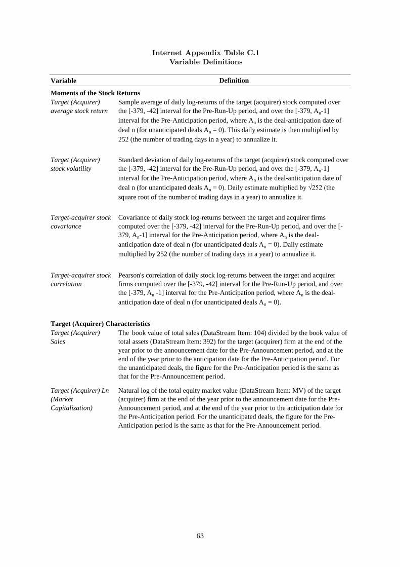
Internet Appendix Table C.1Variable Definitions

Variable

Target (Acquirer)

average stock return

Target (Acquirer)

stock volatility

Target-acquirer stock

covariance

Target-acquirer stock

correlation

Target (Acquirer) Characteristics

Target (Acquirer)

Sales

Target (Acquirer) Ln

(Market

Capitalization)

Definition

Moments of the Stock Returns

Sample average of daily log-returns of the target (acquirer) stock computed over

the [-379, -42] interval for the Pre-Run-Up period, and over the [-379, An-1]

interval for the Pre-Anticipation period, where An is the deal-anticipation date of

deal n (for unanticipated deals An = 0). This daily estimate is then multiplied by

252 (the number of trading days in a year) to annualize it.

Standard deviation of daily log-returns of the target (acquirer) stock computed over

the [-379, -42] interval for the Pre-Run-Up period, and over the [-379, An-1]

interval for the Pre-Anticipation period, where An is the deal-anticipation date of

deal n (for unanticipated deals An = 0). Daily estimate multiplied by √252 (the

square root of the number of trading days in a year) to annualize it.

Covariance of daily stock log-returns between the target and acquirer firms

computed over the [-379, -42] interval for the Pre-Run-Up period, and over the [-

379, An-1] interval for the Pre-Anticipation period, where An is the deal-

anticipation date of deal n (for unanticipated deals An = 0). Daily estimate

multiplied by 252 (the number of trading days in a year) to annualize it.

Pearson's correlation of daily stock log-returns between the target and acquirer

firms computed over the [-379, -42] interval for the Pre-Run-Up period, and over

the [-379, An -1] interval for the Pre-Anticipation period, where An is the deal-

anticipation date of deal n (for unanticipated deals An = 0).

The book value of total sales (DataStream Item: 104) divided by the book value of

total assets (DataStream Item: 392) for the target (acquirer) firm at the end of the

year prior to the announcement date for the Pre-Announcement period, and at the

end of the year prior to the anticipation date for the Pre-Anticipation period. For

the unanticipated deals, the figure for the Pre-Anticipation period is the same as

that for the Pre-Announcement period.

Natural log of the total equity market value (DataStream Item: MV) of the target

(acquirer) firm at the end of the year prior to the announcement date for the Pre-

Announcement period, and at the end of the year prior to the anticipation date for

the Pre-Anticipation period. For the unanticipated deals, the figure for the Pre-

Anticipation period is the same as that for the Pre-Announcement period.

63

Internet Appendix Table C.1 - continued

Variable

Target (Acquirer)

ROE

Target (Acquirer)

Leverage

Target (Acquirer)

Cash holdings

Target (Acquirer)

Tobin's Q

Deal Characteristics

Rumor

Same industry

Relative size

IT industry

The book value of total cash and equivalent (DataStream Item: 375) divided by the

book value of total assets (DataStream Item: 392) for the target (acquirer) firm at

the end of the year prior to the announcement date for the Pre-Announcement

period, and at the end of the year prior to the anticipation date for the Pre-

Anticipation period. For the unanticipated deals, the figure for the Pre-Anticipation

period is the same as that for the Pre-Announcement period.

Definition

The book value of pre-tax profit (DataStream Item: 154) divided by the book value

of total capital employed (DataStream Item: 322) for the target (acquirer) firm at

the end of the year prior to the announcement date for the Pre-Announcement

period, and at the end of the year prior to the anticipation date for the Pre-

Anticipation period. For the unanticipated deals, the figure for the Pre-Anticipation

period is the same as that for the Pre-Announcement period.

The book value of total debt (DataStream Item: 1301) divided by the book value of

total assets (DataStream Item: 392) for the target (acquirer) firm at the end of the

year prior to the announcement date for the Pre-Announcement period, and at the

end of the year prior to the anticipation date for the Pre-Anticipation period. Total

debt is the sum of long and short term debt. For the unanticipated deals, the figure

for the Pre-Anticipation period is the same as that for the Pre-Announcement

period.

The total market value divided by the book value of total assets (DataStream Item:

392) for the target (acquirer) firm at the end of the year prior to the announcement

date for the Pre-Announcement period, and at the end of the year prior to the

anticipation date for the Pre-Anticipation period. The market value of total assets

equals the market value of total equity(DataStream Item: MV) plus the book value

of total liabilities, where the book value of total liabilities is the book value of total

assets minus the book value of total equity (DataStream Item: 322). For the

unanticipated deals, the figure for the Pre-Anticipation period is the same as that

for the Pre-Announcement period.

Indicator that equals 1 if there was a rumor before the first bid-announcement date.

Source: Zephyr

Indicator that equals 1 if the acquirer’s and the target's primary U.S. three-digit SIC

codes coincide. Source: Zephyr

The ratio of the total equity market value of the target to that of the acquirer

(DataStream Item: MV) at the end of the year prior to the announcement date for

the Pre-Announcement period, and at the end of the year prior to the anticipation

date for the Pre-Anticipation period. For the unanticipated deals, the figure for the

Pre-Anticipation period is the same as that for the Pre-Announcement period.

Indicator that equals 1 if at least one of the target’s and the acquirer’s primary SIC

codes is 3571, 3572, 3577 (computer hardware), 3661, 3669 (communications

equipment), 3674 (electronics), 4812, 4813 (telephone communications), 7371,

7372, 7373, 7374, 7375, or 7379 (software). Source: Zephyr

64

Internet Appendix Table C.1 - continued

Variable

Market Volatility

Cash offer

Equity offer

Mixed offer

Announcement-year

dummies

Only Deal Ant.

Dif. Deal and Payment

Ant.

Iden. Deal and

Payment Ant.

Deal-Ant. Quartile 1

Deal-Ant. Quartile 2

Deal-Ant. Quartile 3

Deal-Ant. Quartile 4

Payment-Form Ant.

Quartile 1

Payment-Form Ant.

Quartile 2

Payment-Form Ant.

Quartile 3

Payment-Form Ant.

Quartile 4

Definition

Indicator that equals 1 if the deal is anticipated but not the payment form, and 0

otherwise.

Standard deviation of daily log-returns on the S&P500 index over the [-379, -42]

interval for the Pre-Run-Up period, and over the [-379, An-1] interval for the Pre-

Anticipation period, where An is the deal-anticipation date of deal n (for

unanticipated deals An = 0). Daily estimate multiplied by √252 (the square root of the

number of trading days in a year) to annualize it.

Indicator that equals 1 if the deal is financed through cash only, and 0 otherwise.

Source: Zephyr

Indicator that equals 1 if the deal is financed through the acquirer’s stocks only, and

0 otherwise. Source: Zephyr

Indicator that equals 1 if the deal is financed with both cash and stocks, and 0

otherwise. Source: Zephyr.

Indicators equal to 1 if the first bid offer is announced in year i, and 0 otherwise,

where i = 2003, 2004, 2005 and 2006, respectively. Source: Zephyr.

Anticipation Variables

Indicator that equals 1 if the payment-form-anticipation date lies in the [-318, -210]

interval, and 0 otherwise.

Indicator that equals 1 if the payment-form-anticipation date lies in the [-209, -106]

interval, and 0 otherwise.

Indicator that equals 1 if the payment-form-anticipation date lies in the [-105, -25]

interval, and 0 otherwise.

Indicator that equals 1 if the payment-form-anticipation date lies in the [-24, -1]

interval, and 0 otherwise.

Indicator that equals 1 if the deal-anticipation and the payment-form-anticipation

dates differ, and 0 otherwise.

Indicator that equals 1 if the deal-anticipation and payment-form-anticipation dates

coincide, and 0 otherwise.

Indicator that equals 1 if the deal-anticipation date lies in the [-360, -253] interval,

and 0 otherwise.

Indicator that equals 1 if the deal-anticipation date lies in the [-252, -190] interval,

and 0 otherwise.

Indicator that equals 1 if the deal-anticipation date lies in the [-189, -133] interval,

and 0 otherwise.

Indicator that equals 1 if the deal-anticipation date lies in the [-132, -1] interval, and

0 otherwise.

65

Internet Appendix Table C.2Descriptive Statistics of Deal, Target, and Acquirer Characteristics

This table summarizes the descriptive statistics of the 125 completed M&As’, targets’ and acquirers’

characteristics. The Pre-Run-Up (Pre-Anticipation) period is from Day-379 to Day -42 (to Day An -1)

relative to the first bid announcement date (Day 0). An is the deal-anticipation date of deal n, and for

unanticipated deals An = 0. The firm characteristics during the Pre-Announcement (Pre-Anticipation)

period are taken from the end of the year prior to the announcement (anticipation) date. These two

periods coincide for the unanticipated deals. The variable definitions are given in internet appendix

Table C.1.

Variable Period Mean Std. Dev. 25th 50th 75th

Moments of the Stock Returns

Target average stock return Pre-Run-Up 0.12 0.42 -0.07 0.12 0.36

Pre-Anticipation 0.04 0.78 -0.29 0.02 0.34

Acquirer average stock return Pre-Run-Up 0.17 0.36 -0.01 0.13 0.31

Pre-Anticipation 0.05 0.75 -0.17 0.06 0.26

Target stock volatility Pre-Run-Up 0.54 0.22 0.38 0.51 0.68

Pre-Anticipation 0.59 0.26 0.41 0.55 0.71

Acquirer stock volatility Pre-Run-Up 0.42 0.21 0.29 0.38 0.51

Pre-Anticipation 0.47 0.25 0.29 0.43 0.59

Target-acquirer stock covariance Pre-Run-Up 0.05 0.06 0.01 0.03 0.07

Pre-Anticipation 0.06 0.08 0.01 0.03 0.08

Target-acquirer stock correlation Pre-Run-Up 0.23 0.19 0.08 0.19 0.34

Pre-Anticipation 0.22 0.20 0.07 0.20 0.34

Target Characteristics

Sales Pre-Announcement 1.08 1.03 0.53 0.90 1.27

Pre-Anticipation 1.05 0.97 0.54 0.83 1.29

Ln (Market Capitalization) Pre-Announcement 19.67 1.69 18.27 19.39 20.81

Pre-Anticipation 19.56 1.71 18.12 19.31 20.51

ROE Pre-Announcement -0.03 0.59 -0.05 0.08 0.17

Pre-Anticipation -0.08 0.60 -0.16 0.05 0.15

Leverage Pre-Announcement 0.09 0.15 0 0.02 0.12

Pre-Anticipation 0.10 0.15 0 0.03 0.13

Cash holdings Pre-Announcement 0.36 0.25 0.13 0.34 0.54

Pre-Anticipation 0.34 0.26 0.10 0.30 0.53

Tobin's Q Pre-Announcement 2.32 2.01 1.15 1.78 2.52

Pre-Anticipation 2.32 2.24 1.13 1.65 2.58

Acquirer Characteristics

Sales Pre-Announcement 0.90 0.81 0.43 0.71 1.11

Pre-Anticipation 0.92 0.90 0.39 0.73 1.11

Ln (Market Capitalization) Pre-Announcement 21.58 1.84 20.21 21.41 22.71

Pre-Anticipation 21.51 1.90 20.21 21.40 22.87

ROE Pre-Announcement 0.07 0.24 0.02 0.09 0.18

Pre-Anticipation 0.05 0.36 -0.02 0.08 0.18

Percentile

66

Internet Appendix Table C.2 - continued

Variable Period Mean Std. Dev. 25th 50th 75th

Leverage Pre-Announcement 0.16 0.18 0.003 0.12 0.25

Pre-Anticipation 0.17 0.18 0.01 0.13 0.26

Cash holdings Pre-Announcement 0.24 0.22 0.05 0.19 0.36

Pre-Anticipation 0.24 0.23 0.04 0.18 0.40

Tobin's Q Pre-Announcement 2.11 1.44 1.15 1.56 2.53

Pre-Anticipation 2.13 1.62 1.05 1.49 2.60

Deal Characteristics

Rumor 0.17 0.38 0 0 0

Same industry 0.59 0.49 0 1 1

Relative size Pre-Announcement 0.46 0.81 0.05 0.18 0.50

Pre-Anticipation 0.43 0.69 0.06 0.24 0.50

IT industry 0.40 0.49 0 0 1

Market Volatility Pre-Run-Up 0.17 0.08 0.11 0.13 0.26

Pre-Anticipation 0.15 0.06 0.11 0.12 0.20

Cash offer 0.43 0.50 0 0 1

Equity offer 0.26 0.44 0 0 1

Mixed offer 0.31 0.46 0 0 1

Announced in 2003 0.22 0.41 0 0 0

Announced in 2004 0.33 0.47 0 0 1

Announced in 2005 0.31 0.47 0 0 1

Announced in 2006 0.14 0.34 0 0 0

Anticipation Variables

Only Deal Ant. 0.25 0.43 0 0 0

Dif. Deal and Payment Ant. 0.26 0.44 0 0 1

Iden. Deal and Payment Ant. 0.36 0.48 0 0 1

Deal-Ant. Quartile 1 0.22 0.42 0 0 0

Deal-Ant. Quartile 2 0.21 0.41 0 0 0

Deal-Ant. Quartile 3 0.22 0.41 0 0 0

Deal-Ant. Quartile 4 0.22 0.41 0 0 0

Payment-Form Ant. Quartile 1 0.16 0.37 0 0 0

Payment-Form Ant. Quartile 2 0.15 0.36 0 0 0

Payment-Form Ant. Quartile 3 0.15 0.36 0 0 0

Payment-Form Ant. Quartile 4 0.15 0.36 0 0 0

Percentile

67

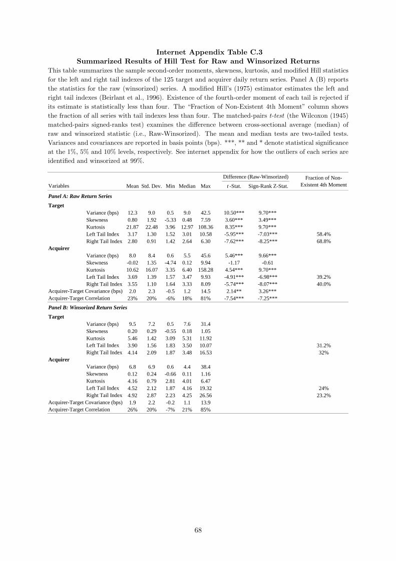
Internet Appendix Table C.3Summarized Results of Hill Test for Raw and Winsorized Returns

This table summarizes the sample second-order moments, skewness, kurtosis, and modified Hill statistics

for the left and right tail indexes of the 125 target and acquirer daily return series. Panel A (B) reports

the statistics for the raw (winsorized) series. A modified Hill’s (1975) estimator estimates the left and

right tail indexes (Beirlant et al., 1996). Existence of the fourth-order moment of each tail is rejected if

its estimate is statistically less than four. The “Fraction of Non-Existent 4th Moment” column shows

the fraction of all series with tail indexes less than four. The matched-pairs t-test (the Wilcoxon (1945)

matched-pairs signed-ranks test) examines the difference between cross-sectional average (median) of

raw and winsorized statistic (i.e., Raw-Winsorized). The mean and median tests are two-tailed tests.

Variances and covariances are reported in basis points (bps). ***, ** and * denote statistical significance

at the 1%, 5% and 10% levels, respectively. See internet appendix for how the outliers of each series are

identified and winsorized at 99%.

Mean Std. Dev. Min Median Max t -Stat. Sign-Rank Z-Stat.

Target

Variance (bps) 12.3 9.0 0.5 9.0 42.5 10.50*** 9.70***

Skewness 0.80 1.92 -5.33 0.48 7.59 3.60*** 3.49***

Kurtosis 21.87 22.48 3.96 12.97 108.36 8.35*** 9.70***

Left Tail Index 3.17 1.30 1.52 3.01 10.58 -5.95*** -7.03*** 58.4%

Right Tail Index 2.80 0.91 1.42 2.64 6.30 -7.62*** -8.25*** 68.8%

Acquirer

Variance (bps) 8.0 8.4 0.6 5.5 45.6 5.46*** 9.66***

Skewness -0.02 1.35 -4.74 0.12 9.94 -1.17 -0.61

Kurtosis 10.62 16.07 3.35 6.40 158.28 4.54*** 9.70***

Left Tail Index 3.69 1.39 1.57 3.47 9.93 -4.91*** -6.98*** 39.2%

Right Tail Index 3.55 1.10 1.64 3.33 8.09 -5.74*** -8.07*** 40.0%

Acquirer-Target Covariance (bps) 2.0 2.3 -0.5 1.2 14.5 2.14** 3.26***

Acquirer-Target Correlation 23% 20% -6% 18% 81% -7.54*** -7.25***

Target

Variance (bps) 9.5 7.2 0.5 7.6 31.4

Skewness 0.20 0.29 -0.55 0.18 1.05

Kurtosis 5.46 1.42 3.09 5.31 11.92

Left Tail Index 3.90 1.56 1.83 3.50 10.07 31.2%

Right Tail Index 4.14 2.09 1.87 3.48 16.53 32%

Acquirer

Variance (bps) 6.8 6.9 0.6 4.4 38.4

Skewness 0.12 0.24 -0.66 0.11 1.16

Kurtosis 4.16 0.79 2.81 4.01 6.47

Left Tail Index 4.52 2.12 1.87 4.16 19.32 24%

Right Tail Index 4.92 2.87 2.23 4.25 26.56 23.2%

Acquirer-Target Covariance (bps) 1.9 2.2 -0.2 1.1 13.9

Acquirer-Target Correlation 26% 20% -7% 21% 85%

Difference (Raw-Winsorized) Fraction of Non-

Existent 4th Moment Variables

Panel A: Raw Return Series

Panel B: Winsorized Return Series

68

Internet Appendix Table D.1Summarized Results of Tests for Detecting Shifts in Each Second-Order MomentThis table summarizes the result of performing various structural break tests for detecting multiple

shifts in the second-order moments of the daily acquirer and target return series. The total sample

consists of 125 completed acquisitions and splits into 54 cash, 33 equity and 38 mixed-payment bids.

The pre-announcement period is from Day -379 to Day -1 relative to the announcement day (= 0). The

post-announcement period is from the announcement day through to the delisting of the target shares.

Each of the 125 daily acquirer and target return series is sequentially adjusted for outliers, breaks in the

mean, and non-zero mean (see explanation in the caption of Table 4). The ICSS test detects the number

and location of significant shifts in the unconditional variance of each target and acquirer return series.

The Bai and Perron (BP) (Galeano and Wied, GW) test detects the number and location of signifi-

cant shifts in the unconditional daily-realized covariance (the unconditional correlation) of the acquirer

and target return series. The “Fraction of Total Deals” column reports the fraction of total deals for

which the breaks are either significant or identified as Anticipation dates. The one-way ANOVA tests

the equality-of-average-break-dates across payment subsamples. All the above tests are two-tailed tests.

***, ** and * denote statistical significance at the 1%, 5% and 10% levels, respectively. See internet

appendix for how Target, Acquirer, and Payment-Form-Anticipation dates are identified.

Variables Mean Std. Dev. Min Median Max

Total 122 71.2% -125.8 106.8 -367 -119 46

Pre-Announcement 94 56.8% -165 90 -367 -168 -2

Post-Announcement 28 22.4% 5.6 12.2 0 0 46

Total 70 56.0% -180.9 89.5 -367 -193 -2 0.46

Cash 26 48.1% -168.8 94.8 -367 -181 -2

Equity 21 63.6% -194.0 90.5 -349 -222 -26

Mixed 23 60.5% -182.8 84.5 -318 -181 -22

Total 112 65.6% -177.7 95.7 -359 -189 62

Pre-Announcement 107 64.8% -188.1 84.4 -359 -193 -1

Post-Announcement 5 4.0% 45.2 16.3 25 51 62

Total 81 64.8% -206.2 76.5 -359 -206 -32 1.40

Cash 34 63.0% -218.0 71.0 -357 -216 -85

Equity 25 75.6% -185.4 89.8 -359 -183 -32

Mixed 22 57.9% -211.6 66.1 -334 -218 -78

Acquirer Variance

Acquirer-Anticipation

Target Variance

Target-Anticipation

Number

of Breaks

Fraction of

Total Deals

Distribution of Break Dates Relative to the

Announcement Day (= 0)F-Value

ANOVA

ICSS Test

69

Internet Appendix Table D.1 - continued

Variables Mean Std. Dev. Min Median Max

Total 58 36% -128.9 127.7 -341 -96 101

Pre-Announcement 45 28.8% -171.8 111.5 -341 -169 -1

Post-Announcement 13 10.4% 19.6 33.5 0 2 101

Total 23 18.4% -178.6 116.5 -341 -169 -1 0.28

Cash 14 25.9% -192.3 112.3 -341 -211 -36

Equity 4 12.1% -144.0 160.7 -315 -130 -1

Mixed 5 13.2% -167.8 110.9 -314 -99 -73

Total 35 25.6% -77.2 93.8 -314 -54 58

Pre-Announcement 22 16% -126.0 85.9 -314 -116 -7

Post-Announcement 13 10.4% 5.5 16.0 0 0 58

Payment-Form-Anticipation

Total 15 12.0% -83.2 55.9 -212 -90 -7 0.80

Cash 2 3.7% -108.5 26.2 -127 -109 -90

Equity 7 21.2% -81.6 69.3 -212 -86 -7

Mixed 6 15.8% -76.7 50.3 -134 -81 -16

Fraction of

Total Deals

Distribution of Break Dates Relative to the

Announcement Day (= 0)F-Value

ANOVA

Acquirer-Target Covariance

GW Test

Acquirer-Target Correlation

Payment-Form-Anticipation

BP Test

Number

of Breaks

70

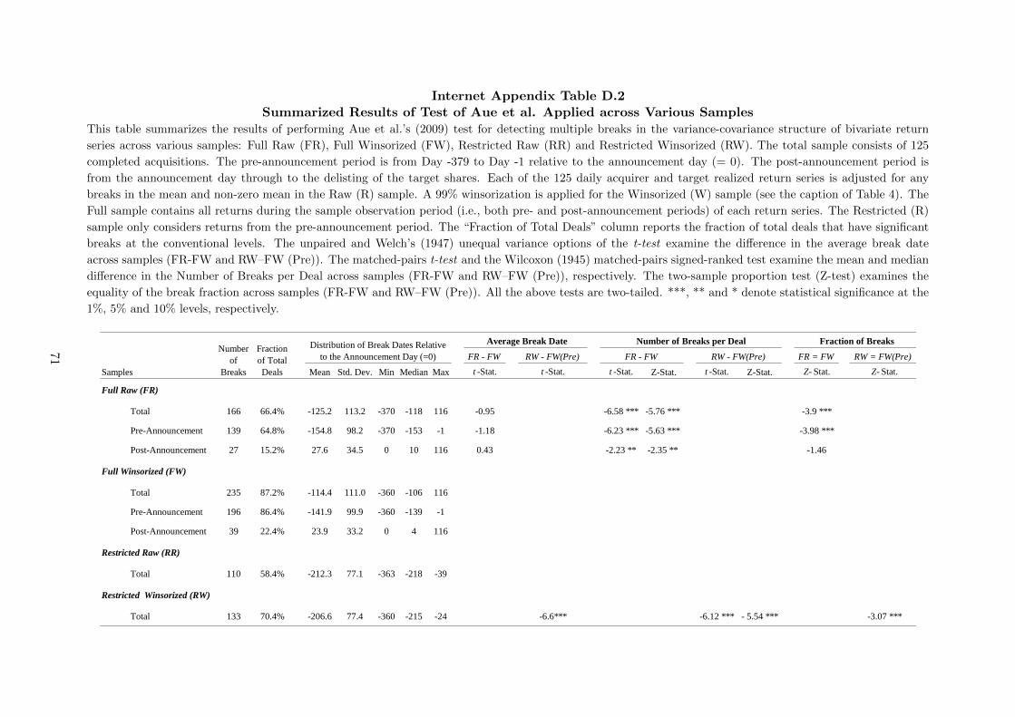
Internet Appendix Table D.2Summarized Results of Test of Aue et al. Applied across Various Samples

This table summarizes the results of performing Aue et al.’s (2009) test for detecting multiple breaks in the variance-covariance structure of bivariate return

series across various samples: Full Raw (FR), Full Winsorized (FW), Restricted Raw (RR) and Restricted Winsorized (RW). The total sample consists of 125

completed acquisitions. The pre-announcement period is from Day -379 to Day -1 relative to the announcement day (= 0). The post-announcement period is

from the announcement day through to the delisting of the target shares. Each of the 125 daily acquirer and target realized return series is adjusted for any

breaks in the mean and non-zero mean in the Raw (R) sample. A 99% winsorization is applied for the Winsorized (W) sample (see the caption of Table 4). The

Full sample contains all returns during the sample observation period (i.e., both pre- and post-announcement periods) of each return series. The Restricted (R)

sample only considers returns from the pre-announcement period. The “Fraction of Total Deals” column reports the fraction of total deals that have significant

breaks at the conventional levels. The unpaired and Welch’s (1947) unequal variance options of the t-test examine the difference in the average break date

across samples (FR-FW and RW–FW (Pre)). The matched-pairs t-test and the Wilcoxon (1945) matched-pairs signed-ranked test examine the mean and median

difference in the Number of Breaks per Deal across samples (FR-FW and RW–FW (Pre)), respectively. The two-sample proportion test (Z-test) examines the

equality of the break fraction across samples (FR-FW and RW–FW (Pre)). All the above tests are two-tailed. ***, ** and * denote statistical significance at the

1%, 5% and 10% levels, respectively.

FR - FW RW - FW(Pre) FR = FW RW = FW(Pre)

Mean Std. Dev. Min Median Max t -Stat. t -Stat. t -Stat. Z-Stat. t -Stat. Z-Stat. Z- Stat. Z- Stat.

Full Raw (FR)

Total 166 66.4% -125.2 113.2 -370 -118 116 -0.95 -6.58 *** -5.76 *** -3.9 ***

Pre-Announcement 139 64.8% -154.8 98.2 -370 -153 -1 -1.18 -6.23 *** -5.63 *** -3.98 ***

Post-Announcement 27 15.2% 27.6 34.5 0 10 116 0.43 -2.23 ** -2.35 ** -1.46

Full Winsorized (FW)

Total 235 87.2% -114.4 111.0 -360 -106 116

Pre-Announcement 196 86.4% -141.9 99.9 -360 -139 -1

Post-Announcement 39 22.4% 23.9 33.2 0 4 116

Restricted Raw (RR)

Total 110 58.4% -212.3 77.1 -363 -218 -39

Restricted Winsorized (RW)

Total 133 70.4% -206.6 77.4 -360 -215 -24 -6.6*** -6.12 *** - 5.54 *** -3.07 ***

FR - FW RW - FW(Pre)

Samples

Number

of

Breaks

Fraction

of Total

Deals

Distribution of Break Dates Relative

to the Announcement Day (=0)

Average Break Date Number of Breaks per Deal Fraction of Breaks

71