BroadieGlassermanKou A Continuity Correction for Discrete Barrier Options
25
Mathematical Finance, Vol. 7, No. 4 (October 1997), 325–348 A CONTINUITY CORRECTION FOR DISCRETE BARRIER OPTIONS MARK BROADIE AND P AUL GLASSERMAN Columbia Business School, New York STEVEN KOU Department of Statistics, University of Michigan The payoff of a barrier option depends on whether or not a specified asset price, index, or rate reaches a specified level during the life of the option. Most models for pricing barrier options assume continuous monitoring of the barrier; under this assumption, the option can often be priced in closed form. Many (if not most) real contracts with barrier provisions specify discrete monitoring instants; there are essentially no formulas for pricing these options, and even numerical pricing is difficult. We show, however, that discrete barrier options can be priced with remarkable accuracy using continuous barrier formulas by applying a simple continuity correction to the barrier. The correction shifts the barrier away from the underlying by a factor of exp(βσ √ 1t ), where β ≈ 0.5826, σ is the underlying volatility, and 1t is the time between monitoring instants. The correction is justified both theoretically and experimentally. KEY WORDS: path-dependent options, Siegmund’s corrected diffusion approximation, level crossing probabilities 1. THE MAIN RESULT 1.1. Introduction A barrier option is activated (knocked in) or extinguished (knocked out) when a specified asset price, index, or rate reaches a specified level. The simplest such options are otherwise standard calls and puts that are knocked in or knocked out by the underlying asset itself. Some variants tie the barrier crossing to one variable and the payoff to another; others specify “binary” payoffs in place of the usual payoffs for calls and puts. Taken together, these are among the most popular options with path-dependent payoffs. The knock-in and knock-out features lower the price of an option, and may provide a payoff distribution that better matches a hedger’s risk or a speculator’s view. Most models of barrier options assume continuous monitoring of the barrier: a knock-in or knock-out is presumed to occur if the barrier is breached at any instant in the life of the option. Under this assumption, Merton (1973) obtained a formula for pricing a knock-out call. Subsequent work on pricing continuously monitored barrier options includes Heynen and Kat (1994a, 1994b), Kunitomo and Ikeda (1992), Rich (1994a, 1994b), and Rubinstein and Reiner (1991). However, a sizable portion of real contracts with barrier features spec- ify fixed times for monitoring of the barrier—typically, daily closings. One article in the trade literature (Derivatives Week 1995a) faults existing pricing models for not addressing Manuscript received September 1995; final revision received April 1996. Address correspondence to the first two authors at Columbia Business School, 415 Uris Hall, New York, NY 10027; e-mail: [email protected]; [email protected], or to the third author at the Dept. of Statistics, University of Michigan, Ann Arbor, MI 48109; e-mail: [email protected]. c 1997 Blackwell Publishers, 350 Main St., Malden, MA 02148, USA, and 108 Cowley Road, Oxford, OX4 1JF, UK. 325
-
Upload
ginovainmona -
Category
Documents
-
view
214 -
download
0
Transcript of BroadieGlassermanKou A Continuity Correction for Discrete Barrier Options

Mathematical Finance, Vol. 7, No. 4 (October 1997), 325–348
A CONTINUITY CORRECTION FOR DISCRETE BARRIER OPTIONS
MARK BROADIE AND PAUL GLASSERMAN
Columbia Business School, New York
STEVEN KOU
Department of Statistics, University of Michigan
The payoff of abarrier option depends on whether or not a specified asset price, index, or ratereaches a specified level during the life of the option. Most models for pricing barrier options assumecontinuous monitoring of the barrier; under this assumption, the option can often be priced in closedform. Many (if not most) real contracts with barrier provisions specify discrete monitoring instants;there are essentially no formulas for pricing these options, and even numerical pricing is difficult. Weshow, however, that discrete barrier options can be priced with remarkable accuracy using continuousbarrier formulas by applying a simple continuity correction to the barrier. The correction shifts thebarrier away from the underlying by a factor of exp(βσ
√1t), whereβ ≈ 0.5826,σ is the underlying
volatility, and1t is the time between monitoring instants. The correction is justified both theoreticallyand experimentally.
KEY WORDS: path-dependent options, Siegmund’s corrected diffusion approximation, level crossingprobabilities
1. THE MAIN RESULT
1.1. Introduction
A barrier optionis activated (knocked in) or extinguished (knocked out) when a specifiedasset price, index, or rate reaches a specified level. The simplest such options are otherwisestandard calls and puts that are knocked in or knocked out by the underlying asset itself.Some variants tie the barrier crossing to one variable and the payoff to another; othersspecify “binary” payoffs in place of the usual payoffs for calls and puts. Taken together,these are among the most popular options with path-dependent payoffs. The knock-in andknock-out features lower the price of an option, and may provide a payoff distribution thatbetter matches a hedger’s risk or a speculator’s view.
Most models of barrier options assume continuous monitoring of the barrier: a knock-inor knock-out is presumed to occur if the barrier is breached atany instant in the life of theoption. Under this assumption, Merton (1973) obtained a formula for pricing a knock-outcall. Subsequent work on pricing continuously monitored barrier options includes Heynenand Kat (1994a, 1994b), Kunitomo and Ikeda (1992), Rich (1994a, 1994b), and Rubinsteinand Reiner (1991). However, a sizable portion of real contracts with barrier features spec-ify fixed times for monitoring of the barrier—typically, daily closings. One article in thetrade literature (Derivatives Week1995a) faults existing pricing models for not addressing
Manuscript received September 1995; final revision received April 1996.Address correspondence to the first two authors at Columbia Business School, 415 Uris Hall, New York,
NY 10027; e-mail: [email protected]; [email protected], or to the thirdauthor at the Dept. of Statistics, University of Michigan, Ann Arbor, MI 48109; e-mail: [email protected].
c© 1997 Blackwell Publishers, 350 Main St., Malden, MA 02148, USA, and 108 Cowley Road, Oxford,OX4 1JF, UK.
325

326 M. BROADIE, P. GLASSERMAN, AND S. KOU
this feature. Another (Derivatives Week1995b) discusses concerns that when monitoringtimes are not specified, extraneous barrier breaches may occur in less liquid markets whilethe major Western markets are closed. Moreover, numerical examples, including those inChance (1994), Flesaker (1992), and Kat and Verdonk (1995), indicate that there can besubstantial price differences between discrete and continuous barrier options, even underdaily monitoring of the barrier. Unfortunately, the exact pricing results available for contin-uous barriers do not extend to the discrete case.1 Even numerical methods using standardlattice techniques or Monte Carlo simulation face significant difficulties in incorporatingdiscrete monitoring, as demonstrated in Broadie, Glasserman, and Kou (1996).
In this paper, we introduce a simple continuity correction for approximate pricing ofdiscrete barrier options. Our method uses formulas for the prices of continuous barrieroptions but shifts the barrier to correct for discrete monitoring. The shift is determinedsolely by the monitoring frequency, the asset volatility, and a constantβ ≈ 0.5826. Itis therefore trivial to implement. Compared with using the unadjusted continuous price,our formula reduces the error fromO(1/
√m) to o(1/
√m), as the number of monitoring
pointsm increases. Numerical results indicate that the approximation is accurate enough tocorrectly price barrier options in all but the most extreme circumstance; i.e., except whenthe price of the underlying asset nearly coincides with the barrier.
Our analysis is based on the usual Black–Scholes market assumptions (Black and Scholes1973). In particular, the asset price{St , t ≥ 0} follows the stochastic differential equation
dS
S= ν dt + σ d Z,(1.1)
whereZ is a standard Wiener process,ν andσ > 0 are constants, andS0 is fixed. Theterm structure is flat, and we letr denote the constant, continuously compounded risk-freeinterest rate. The price of a claim contingent onS is the expected present value of its cashflows under the equivalent martingale measure, which setsν = r in (1.1).
Let H denote the level of the barrier. Anup option hasH > S0 and adownoption hasH < S0; in particular, we always assumeH 6= S0. The asset price reaches the barrier forthe first time at2
τH = inf{t > 0 : St = H};(1.2)
this is an up-crossing ifS0 < H and a down-crossing ifS0 > H . A knock-in call optionwith maturityT and strikeK pays(ST − K )+ at timeT if τH ≤ T and zero otherwise. Itsprice is thus3
e−rT E[(ST − K )+; τH ≤ T ],
the expectation taken with respect to the equivalent martingale measure. For a put option,replace(ST − K )+ with (K − ST )
+, and for knock-out options replace the event{τH ≤ T}
1The price of a discrete barrier option can be expressed in “closed form” in terms of multivariate normalprobabilities. The dimension of the relevant multivariate normal distribution is equal to the number of monitoringinstants. This is typically too large for numerical evaluation.
2Here and in what follows, we adopt the usual convention that the infimum of an empty set is infinity, so thatin particularτH = ∞ if the asset prices never reach the barrier.
3For a random variableX and an eventA, the notationE[X; A] meansE[X1A], with 1A the indicator ofA.

A CONTINUITY CORRECTION FOR DISCRETE BARRIER OPTIONS 327
with its complement{τH > T}. Formulas for pricing these continuously monitored barrieroptions are reviewed in Section 3.
Now suppose the barrier is monitored only at timesi1t , i = 0, 1, . . . ,m, where1t =T/m. Let us writeSi for Si1t , so that{Si , i = 0, 1, . . .} is the asset price at monitoringinstants. Define
τH ={
inf{n > 0 : Sn > H}, S0 < Hinf{n > 0 : Sn < H}, S0 > H.
The price of adiscreteknock-in call option is given by
e−rT E[(Sm − K )+; τH ≤ m];
the same modifications as before yield puts and knock-outs.In general, there are no easily computed closed-form expressions for the prices of these
discrete barrier options. A consequence of our analysis is the obvious conclusion that thediscrete price converges to the continuous price as the monitoring frequency increases,suggesting that the continuous price may be used as a naive approximation. The followingresult shows how to adjust the continuous formula to obtain a far better approximation tothe discrete price.
THEOREM1.1. Let Vm(H) be the price of a discretely monitored knock-in or knock-out down call or up put with barrier H. Let V(H) be the price of the correspondingcontinuously monitored barrier option. Then
Vm(H) = V(He±βσ√
T/m)+ o
(1√m
),(1.3)
where+ applies if H> S0,− applies if H< S0, andβ = −ζ( 12)/√
2π ≈ 0.5826, with ζthe Riemann zeta function.
This result indicates that to use the continuous price as an approximation to the discreteprice, we should first shift the barrier away fromS0 by a factor of exp(βσ
√1t). Numerical
results in Section 2 suggest that the resulting approximation is remarkably accurate.
1.2. A Sketch of the Argument
Sections 3 and 4 and the appendices are devoted to the proof of Theorem 1.1. To givesome insight into the result, we illustrate the argument for an example. Consider abinaryknock-in option paying one dollar if the asset price reachesH at some point in [0, T ] and if attimeT it is belowK , with H > max{S0, K }. A by-product of the analysis in later sections(Corollary 4.1) is that Theorem 1.1 applies to binary barrier options as well. Suppose,for purposes of illustration, thatr − 1
2σ2 = 0, so that under the equivalent martingale
measure logSt has zero drift.4 Defineb andc via the relationsH = S0 exp(bσ√
T) and
4Ito’s lemma applied to (1.1) yieldsd log S= (ν − 12σ
2) dt + σ d Z.

328 M. BROADIE, P. GLASSERMAN, AND S. KOU
K = S0 exp(cσ√
T). Assuming continuous monitoring of the barrier, the value of theoption ise−rT times
P(ST < K , τH ≤ T) = P(log ST < cσ√
T, max0≤t≤T
log St ≥ bσ√
T)
= P(log ST ≥ (2b− c)σ√
T)(1.4)
= 1−Φ(2b− c),(1.5)
whereΦ is the standard normal cumulative distribution function. Equation (1.4) is anapplication of the reflection principle (Karatzas and Shreve 1991, pp. 79–80).
Suppose, now, that for the option to be knocked in, the asset price must reachH at sometime in{0,1t, 21t, . . . ,m1t}, with1t = T/m. Becauser − 1
2σ2 = 0, we may represent
the asset price at these monitoring instants as
Sn = S0eσ√1t Wn, with Wn =
n∑i=1
Zi ,
where theZi are independent standard normal random variables. The price of the optionunder discrete monitoring of the barrier ise−rT times
P(Sm < K , max0≤n≤m
Sn ≥ H) = P(Wm < c√
m, τ ≤ m),
where τ is the first timeW exceedsb√
m. The increments of the random walkW aresymmetrically distributed, so the reflection principle yields
P(Wm < c√
m, τ ≤ m) = P(Wm > 2(b√
m+ Rm)− c√
m),(1.6)
whereRm4= Wτ − b
√m is theovershootabove levelb
√m (see Figure 1.1). Notice that
P(Wm > x√
m) = 1− Φ(x). Applying this to (1.6) and treatingWm and Rm as thoughthey were independent we get
P(Wm > 2(b√
m+ Rm)− c√
m) ≈ E
[1−Φ(2
(b+ Rm√
m
)− c
)].(1.7)
Expanding in a formal Taylor series withϕ denoting the standard normal density, and usingthe fact (to be reviewed in Section 4.3) thatE[Rm] → β, we get
P(Wm > 2(b√
m+ Rm)− c√
m) ≈ E
[1−Φ(2b− c)− 2Rm√
mϕ(2b− c)+ o
(1√m
)]≈ 1−Φ(2b− c)− 2√
mE[Rm]ϕ(2b− c)+ o
(1√m
)

A CONTINUITY CORRECTION FOR DISCRETE BARRIER OPTIONS 329
}Rm
�mc
mb
τ
( )2 −+ mcRmb mS
t
FIGURE 1.1. Overshoot and reflection principle illustration.
= 1−Φ(2b− c)− 2β√mϕ(2b− c)+ o
(1√m
)= 1−Φ(2
(b+ β√
m
)− c
)+ o
(1√m
).
In light of (1.5), this is
P(ST < K , τH exp(βσ√1t) ≤ T)+ o
(1√m
),
and thus agrees, up too(1/√
m), with the price of a continuously monitored barrier optionknocked in at levelH exp(βσ
√1t). The differenceHeβσ
√1t − H may be viewed as
an approximation to the amount by which the asset price exceeds the barrier at the firstmonitoring instant at which it is above the barrier.
The heuristic argument just sketched points out the key steps in proving Theorem 1.1rigorously: we find a suitable representation of the discrete price, expand it in a Taylor series,evaluate the limits of the coefficients asm→ ∞, and identify the resulting expression asan expansion of the continuous price. Evaluation of the limits of coefficients requiresconsideration of the joint limit of the overshoot and the barrier-crossing time; the necessaryasymptotic independence result is given in Section 4.3, and this may be viewed as therigorous counterpart of (1.7). Handling ordinary barrier options instead of just binaryoptions requires consideration of integrals of the probabilities outlined above.
Continuity corrections for level-crossing probabilities of random walks have a long his-tory in sequential analysis and, to a lesser extent, in risk theory. Key references fromthe statistical literature are Chernoff (1965), Siegmund (1979, 1985), Siegmund and Yuh

330 M. BROADIE, P. GLASSERMAN, AND S. KOU
(1982), and Woodroofe (1982); for developments in risk theory see Asmussen (1989). Weespecially build on the work of Siegmund and Yuh. Also in the context of sequentialanalysis, Chernoff and Petkau (1986) have shown that a boundary correction improves thenumerical solution of an optimal stopping problem based on a binomial approximation toa diffusion. Recently, AitSahlia (1995) has analyzed a similar technique in the pricing ofAmerican options (without barriers).
2. PERFORMANCE OF THE CORRECTED BARRIER APPROXIMATION
Before proceeding with the main proof, we present numerical results to indicate the accuracyof the corrected barrier approximation given in equation (1.3). Table 2.1 compares theapproximation (and two related approximations to be described shortly) with the true valuefor different levels of the barrierH . The options considered are down-and-out call options,i.e., S0 > H , and the option becomes worthless ifS crosses the barrier before the optionexpires at timeT . The “true” value is determined from a trinomial procedure modified inseveral ways to specifically handle discrete barriers and is fully described in Broadie et al.(1996). This numerical procedure has an average accuracy of about 0.001 for this range ofparameters.
Table 2.1 and later tables show that the continuous barrier price can differ from the discretebarrier price by economically significant amounts. For example, forH = 97 in Table 2.1,the continuous barrier price is $3.06 while the discrete barrier option with daily monitoringis worth 25% more ($3.83). The prices under approximation (1) in the tables result from thecorrected continuous barrier formula suggested by Theorem 1.1. The relative absolute errorof this formula is less than 0.1% forH ≤ 98; overall, this formula is remarkably accurateexcept in extreme cases withH very close toS0. It can be evaluated very fast (more than10,000/sec on an Intel Pentium 133 MHz processor), while the procedure used to computethe true value to comparable accuracy is many orders of magnitude slower (approximatelyone hour on the same processor).5
Table 2.1 shows results for two other approximations. Approximation (2) uses a formulaof Heynen and Kat (1994b) for continuouspartial barrier options, i.e., options whosebarriers are monitored throughout a time interval [0, t1] or [t1, T ], with 0 < t1 < T . Thefirst monitoring point for a discrete barrier option does not occur until1t , suggesting anapproximation that shifts the barrier in the formula for a partial barrier option monitoredduring [1t, T ]. Specifically, approximation (2) setst1 = 1t and shifts the barrier inequation (9) on p. 259 of Heynen and Kat (1994b). It can be evaluated in about the same(negligible) computing time as the first approximation. Although correcting the continuousbarrier formula (approximation (1)) leads to small underpricing in some cases, the correctedpartial barrier formula (approximation (2)) leads to small overpricing in these cases.
The modified corrected partial barrier approximation (3) in Table 2.1 is a further heuristicthat attempts to compromise between the slight underpricing and overpricing observed with(1) and (2). It does so by adjusting the beginning of the partial barrier tot1 = 0.581t . (Thefactor 0.58 was found experimentally to be the best among a few different values tried.)In most of the test cases, this heuristic had the smallest error of the three approximations.It is worth emphasizing, however, that only approximation (1) is rigorously supported; anattempt to justify a refinement of (1) would involve the daunting task of carrying out the
5In order to compute the true value to within 0.001 on average, we needed to run a modified trinomial routineusing 80,000 time steps. The large number of steps required for this accuracy is quite computationally intensive.

A CONTINUITY CORRECTION FOR DISCRETE BARRIER OPTIONS 331
TABLE 2.1Down-and-Out Call Option Price Results,m= 50 barrier points
Corrected Corrected Modifiedcontinuous partial corrected Relative error
Continuous barrier barrier partial (in percent)Barrier barrier (1) (2) (3) True (1) (2) (3)
85 6.308 6.322 6.322 6.322 6.322 0.0 0.0 0.086 6.283 6.306 6.306 6.306 6.306 0.0 0.0 0.087 6.244 6.281 6.281 6.281 6.281 0.0 0.0 0.088 6.185 6.242 6.242 6.242 6.242 0.0 0.0 0.089 6.099 6.184 6.184 6.184 6.184 0.0 0.0 0.090 5.977 6.098 6.098 6.098 6.098 0.0 0.0 0.091 5.808 5.977 5.977 5.977 5.977 0.0 0.0 0.092 5.579 5.810 5.810 5.810 5.810 0.0 0.0 0.093 5.277 5.585 5.585 5.585 5.584 0.0 0.0 0.094 4.888 5.288 5.288 5.288 5.288 0.0 0.0 0.095 4.398 4.907 4.907 4.907 4.907 0.0 0.0 0.096 3.792 4.428 4.429 4.428 4.427 0.0 0.1 0.097 3.060 3.836 3.845 3.837 3.834 0.1 0.3 0.198 2.189 3.121 3.160 3.129 3.126−0.2 1.1 0.199 1.171 2.271 2.408 2.321 2.337−2.8 3.0 −0.6
Option parameters:S0 = 100,K = 100,σ = 0.30,r = 0.10, andT = 0.2. Assuming 250 trading days per year,m= 50 barrier points roughly corresponds to daily monitoring of the barrier.
expansions in Sections 3 and 4 to one more term. Also, approximations (2) and (3) areslightly more complicated to implement than approximation (1).
Table 2.2 shows that the approximations degrade slowly as the number of monitoringpoints decreases. Indeed, even though Theorem 1.1 is based on the limit asm increasesto infinity, the approximation is quite accurate even form = 5, in marked contrast to thecontinuous price. Table 2.3 shows results for high asset volatility (σ = 0.6), long maturity(T = 2), and higher strike (K = 110). The overall performance of the approximationsremains excellent, except when the barrier is very close to the underlying asset price. In thiscase, the relative errors are slightly larger with higher volatility and longer time to maturityand are slightly lower with a higher strike (compared to Table 2.1).
Option price derivatives (e.g., “delta” =∂V/∂S0) are of particular importance to practi-tioners for hedging and risk management. Although this case is not covered by Theorem 1.1,the correction can be applied to the continuous delta formula as well. Table 2.4 shows howthe deltas of the three approximations compare to the true delta (determined through exten-sive numerical computations). Relative absolute errors are less than 0.1% forH ≤ 97 forapproximation (1). Delta approximations (2) and (3) are better than (1) forH very closeto S0.
Next we consider a two-state example where the payoff of the option is determined by onestate variable and the knock in and or knock out is determined by a second state variable—for example, options on stocks or stock indices which are knocked out if a currency reachesa barrier trade in the over-the-counter market. Rich (1996) models options with defaultrisk in this framework. Heynan and Kat (1994a) and Rich (1996) derive formulas for such

332 M. BROADIE, P. GLASSERMAN, AND S. KOU
TABLE 2.2Down-and-Out Call Option Price Results, varyingm
Corrected Corrected Modifiedcontinuous partial corrected Relative error
Continuous barrier barrier partial (in percent)m Barrier barrier (1) (2) (3) True (1) (2) (3)
85 6.308 6.327 6.327 6.327 6.326 0.0 0.0 0.087 6.244 6.293 6.293 6.293 6.292 0.0 0.0 0.089 6.099 6.210 6.210 6.210 6.210 0.0 0.0 0.091 5.808 6.033 6.033 6.033 6.032 0.0 0.0 0.0
25 93 5.277 5.688 5.688 5.688 5.688 0.0 0.0 0.095 4.398 5.084 5.088 5.084 5.081 0.0 0.1 0.097 3.060 4.113 4.154 4.120 4.116−0.1 0.9 0.199 1.171 2.673 2.923 2.779 2.813−5.0 3.9 −1.2
85 6.308 6.337 6.338 6.337 6.337 0.0 0.0 0.087 6.244 6.323 6.323 6.323 6.321 0.0 0.0 0.089 6.099 6.284 6.287 6.285 6.281 0.1 0.1 0.191 5.808 6.194 6.205 6.195 6.187 0.1 0.3 0.1
5 93 5.277 6.004 6.043 6.011 6.000 0.1 0.7 0.295 4.398 5.646 5.760 5.676 5.671−0.5 1.6 0.197 3.060 5.028 5.323 5.141 5.167−2.7 3.0 −0.599 1.171 4.050 4.724 4.392 4.489−9.8 5.2 −2.2
Option parameters:S0 = 100,K = 100,σ = 0.30,r = 0.10, andT = 0.2.
two-state options when the barrier is continuously monitored. More specifically, supposethat the risk-neutralized asset price processes aredSi = Si (r dt + σi d Zi ), i = 1, 2, whereZ1 andZ2 have a constant correlationρ. Table 2.5 presents results for a two-asset discretebarrier down-and-out call option. The payoff of the option is(S1
T − K )+ if S2 is greaterthan H at all monitoring times. The “true” price is more difficult to determine becauseof the extra dimension involved, but the two-dimensional trinomial procedure used has anaverage accuracy of about 0.003 for this range of parameters. Table 2.5 shows that thecorrected continuous barrier formula is very accurate as long as the barrier is not too closeto the initial price of asset 2.
The previous examples involved down-call options, i.e., options that are knocked outwhen an asset pricedecreasesto a barrier level, but whose payoff is positive if the terminalasset price isabovea strike level. Table 2.6 gives results for up call options (not covered byTheorem 1.1). The results indicate that the corrected barrier formula works well for theseoptions, though perhaps not as well as for down calls. Corrected versions of the continuouspartial barrier formulas in Heynen and Kat (1994b) could also be used to approximate thediscrete barrier price.
3. THE CONTINUOUS PRICE
The purpose of this section is to derive expressions for the continuous priceV(H) and itsderivative. In this and the remaining sections, we detail the case of the down-and-in call,

A CONTINUITY CORRECTION FOR DISCRETE BARRIER OPTIONS 333
TABLE 2.3Down-and-Out Call Option Price Results, varyingσ , T , andK
Corrected Corrected Modifiedcontinuous partial corrected Relative error
Continuous barrier barrier partial (in percent)Panel Barrier barrier (1) (2) (3) True (1) (2) (3)
85 10.048 10.505 10.505 10.505 10.505 0.0 0.0 0.087 9.404 10.020 10.020 10.020 10.020 0.0 0.0 0.089 8.578 9.384 9.384 9.384 9.383 0.0 0.0 0.091 7.547 8.573 8.574 8.573 8.572 0.0 0.0 0.0
A 93 6.293 7.566 7.572 7.566 7.563 0.0 0.1 0.095 4.803 6.346 6.379 6.351 6.344 0.0 0.6 0.197 3.067 4.900 5.033 4.937 4.941−0.8 1.9 −0.199 1.084 3.219 3.638 3.414 3.475−7.4 4.7 −1.8
85 18.856 20.821 20.822 20.821 20.819 0.0 0.0 0.087 17.232 19.573 19.577 19.574 19.571 0.0 0.0 0.089 15.361 18.120 18.133 18.121 18.114 0.0 0.1 0.091 13.227 16.446 16.487 16.450 16.436 0.1 0.3 0.1
B 93 10.815 14.534 14.650 14.553 14.537 0.0 0.8 0.195 8.111 12.371 12.657 12.446 12.451−0.6 1.7 0.097 5.104 9.945 10.576 10.183 10.254−3.0 3.1 −0.799 1.782 7.243 8.499 7.874 8.061−10.1 5.4 −2.3
85 2.494 2.496 2.496 2.496 2.496 0.0 0.0 0.087 2.485 2.491 2.491 2.491 2.491 0.0 0.0 0.089 2.459 2.475 2.475 2.475 2.475 0.0 0.0 0.091 2.394 2.433 2.433 2.433 2.433 0.0 0.0 0.0
C 93 2.250 2.336 2.337 2.337 2.336 0.0 0.0 0.095 1.964 2.136 2.136 2.136 2.135 0.0 0.0 0.097 1.446 1.757 1.761 1.757 1.756 0.1 0.3 0.199 0.591 1.105 1.171 1.129 1.136−2.7 3.0 −0.6
Option parameters:S0 = 100 andr = 0.10. There arem = 50 barrier points (daily monitoring). Panel A hasσ = 0.6, K = 100,T = 0.2; Panel B hasT = 2.0, σ = 0.3, K = 100; and Panel C hasK = 110,σ = 0.3,T = 0.2.
the other cases following with only minor modifications. Thus,
V(H) = e−rT E[(ST − K )+; τH < T ],
with H < S0 andH < K . We defineW to be a Wiener process with variance parameterσ 2
and driftµ4= r − 1
2σ2. This allows us to represent the asset price asSt = S0 exp(Wt ) and
then work withW rather thanS. The barrier is breached whenW hitsa4= log(H/S0); i.e.,
τH = inf{t ≥ 0 : S0eWt ≤ H}= inf{t ≥ 0 : Wt ≤ a}.

334 M. BROADIE, P. GLASSERMAN, AND S. KOU
TABLE 2.4Down-and-Out Call Option Delta Results,m= 50 barrier points
Corrected Corrected Modifiedcontinuous partial corrected Relative error
Continuous barrier barrier partial (in percent)Barrier barrier (1) (2) (3) True (1) (2) (3)
85 0.594 0.591 0.591 0.591 0.591 0.0 0.0 0.086 0.599 0.594 0.594 0.594 0.594 0.0 0.0 0.087 0.607 0.600 0.600 0.600 0.600 0.0 0.0 0.088 0.618 0.607 0.607 0.607 0.607 0.0 0.0 0.089 0.633 0.618 0.618 0.618 0.618 0.0 0.0 0.090 0.653 0.633 0.633 0.633 0.633 0.0 0.0 0.091 0.679 0.653 0.653 0.653 0.653 0.0 0.0 0.092 0.711 0.678 0.678 0.678 0.678 0.0 0.0 0.093 0.752 0.710 0.710 0.710 0.711 0.0 0.0 0.094 0.800 0.750 0.750 0.750 0.750 0.0 0.0 0.095 0.857 0.798 0.797 0.798 0.798 0.0−0.1 0.096 0.921 0.853 0.851 0.853 0.854−0.1 −0.4 −0.297 0.994 0.917 0.904 0.915 0.917 0.0−1.4 −0.298 1.073 0.988 0.938 0.972 0.966 2.2−2.9 0.699 1.158 1.066 0.922 0.988 0.958 11.3−3.7 3.1
Option parameters:S0 = 100, K = 100,σ = 0.30, r = 0.10, andT = 0.2. There arem = 50 barrier points(daily monitoring).
Define
BSC(s) = e−rT E[(seWT − K )+],
the Black–Scholes price of a call option as a function of the initial asset price. Then wehave
PROPOSITION3.1. For a down-and-in call,
V(H) =(
H
S0
)(2r/σ 2)−1
BSC(H2/S0)(3.1)
= e2µa/σ 2BSC(S0e2a)(3.2)
= e−rT e2µa/σ 2∫ ∞
[log(K/S0)]/σ√
T
(1−Φ(x − µ
√T
σ− 2a
σ√
T
))(3.3)
× S0exσ√
Tσ√
T dx.
Proof. The first identity is a consequence of Merton’s (1973, eqn. (55)) formula for abarrier option; this particular representation is from Boyle and Lau (1994). The secondidentity restates the first becausea = log(H/S0). To get the last identity, write the Black–

A CONTINUITY CORRECTION FOR DISCRETE BARRIER OPTIONS 335
TABLE 2.5Two-Asset Down-and-Out Call Option Price Results,m= 50 barrier points
Corrected RelativeContinuous continuous error
Barrier barrier barrier True (in percent)
85 5.893 5.986 5.985 0.086 5.772 5.887 5.886 0.087 5.626 5.766 5.765 0.088 5.452 5.621 5.620 0.089 5.246 5.448 5.447 0.090 5.005 5.244 5.243 0.091 4.726 5.005 5.005 0.092 4.404 4.729 4.729 0.093 4.038 4.412 4.413 0.094 3.623 4.051 4.052 0.095 3.158 3.643 3.645 −0.196 2.639 3.185 3.187 −0.197 2.066 2.676 2.679 −0.198 1.435 2.112 2.121 −0.499 0.747 1.493 1.542 −3.2
Option parameters: Initial assets prices areS1 = S2 = 100, K = 100,σ1 = σ2 = 0.30, r = 0.10, ρ = 0.5, andT = 0.2. There arem = 50barrier points (daily monitoring). The option is knocked out ifS2 hits thebarrier at a monitoring time. The option payoff is(S1
T − K )+ at timeT ifthe option has not been knocked out.
TABLE 2.6Up-and-Out Call Option Price Results,m= 50 barrier points
Corrected RelativeContinuous continuous error
Barrier barrier barrier True (in percent)
155 12.775 12.905 12.894 0.1150 12.240 12.448 12.431 0.1145 11.395 11.707 11.684 0.2140 10.144 10.581 10.551 0.3135 8.433 8.994 8.959 0.4130 6.314 6.959 6.922 0.5125 4.012 4.649 4.616 0.7120 1.938 2.442 2.418 1.0115 0.545 0.819 0.807 1.5
Option parameters:S0 = 110,K = 100,σ = 0.30,r = 0.10, andT = 0.2.
336 M. BROADIE, P. GLASSERMAN, AND S. KOU
Scholes price as
BSC(s) = e−rT E[(seWT − K )+]
= e−rT∫ ∞−∞(sey − K )+
1
σ√
Tϕ
(y− µT
σ√
T
)dy
= e−rT∫ ∞
log(K/s)
(1−Φ( y− µT
σ√
T
))sey dy
using integration by parts. Apply this to (3.2) to get
V(H) = e−rT e2µa/σ 2∫ ∞
log(K/S0e2a)
(1−Φ( y− µT
σ√
T
))S0e2aey dy,
and make the substitutionx = (y+ 2a)/(σ√
T) to get (3.3).
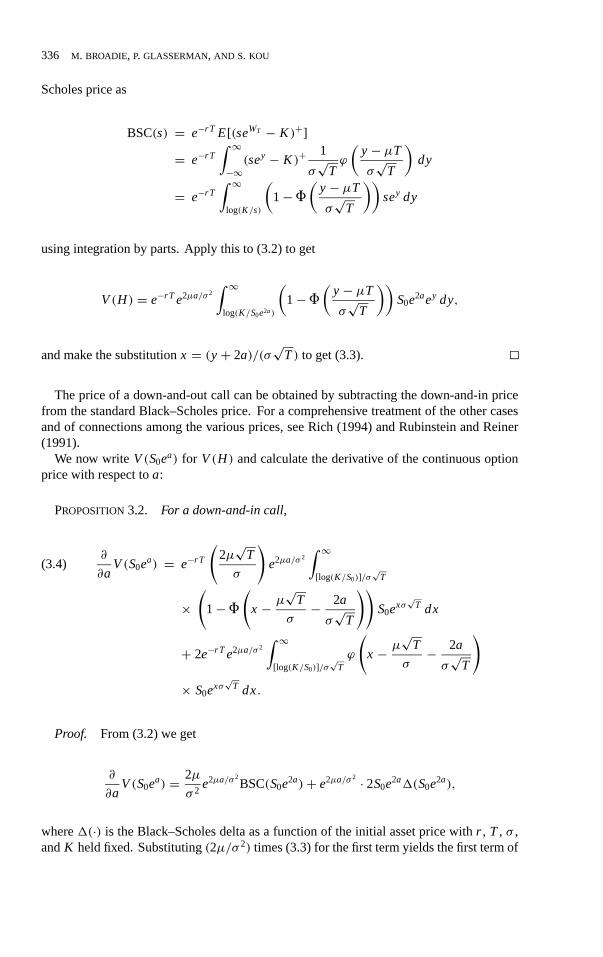
The price of a down-and-out call can be obtained by subtracting the down-and-in pricefrom the standard Black–Scholes price. For a comprehensive treatment of the other casesand of connections among the various prices, see Rich (1994) and Rubinstein and Reiner(1991).
We now writeV(S0ea) for V(H) and calculate the derivative of the continuous optionprice with respect toa:
PROPOSITION3.2. For a down-and-in call,
∂
∂aV(S0ea) = e−rT
(2µ√
T
σ
)e2µa/σ 2
∫ ∞[log(K/S0)]/σ
√T
(3.4)
×(
1−Φ(x − µ√
T
σ− 2a
σ√
T
))S0exσ
√T dx
+ 2e−rT e2µa/σ 2∫ ∞
[log(K/S0)]/σ√
Tϕ
(x − µ
√T
σ− 2a
σ√
T
)× S0exσ
√T dx.
Proof. From (3.2) we get
∂
∂aV(S0ea) = 2µ
σ 2e2µa/σ 2
BSC(S0e2a)+ e2µa/σ 2 · 2S0e2a1(S0e2a),
where1(·) is the Black–Scholes delta as a function of the initial asset price withr , T , σ ,andK held fixed. Substituting(2µ/σ 2) times (3.3) for the first term yields the first term of
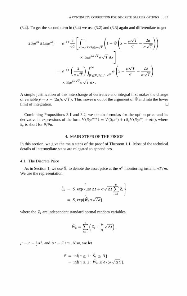
A CONTINUITY CORRECTION FOR DISCRETE BARRIER OPTIONS 337
(3.4). To get the second term in (3.4) we use (3.2) and (3.3) again and differentiate to get
2S0e2a1(S0e2a) = e−rT ∂
∂a
[∫ ∞[log(K/S0)]/σ
√T
(1−Φ(x − µ
√T
σ− 2a
σ√
T
))
× S0exσ√
Tσ√
T dx
]
= e−rT
(2
σ√
T
)∫ ∞[log(K/S0)]/σ
√Tϕ
(x − µ
√T
σ− 2a
σ√
T
)× S0exσ
√Tσ√
T dx.
A simple justification of this interchange of derivative and integral first makes the changeof variabley = x− (2a/σ
√T). This movesa out of the argument ofΦ and into the lower
limit of integration.
Combining Propositions 3.1 and 3.2, we obtain formulas for the option price and itsderivative in expressions of the formV(S0ea+ε) = V(S0ea) + ε∂aV(S0ea) + o(ε), where∂a is short for∂/∂a.
4. MAIN STEPS OF THE PROOF
In this section, we give the main steps of the proof of Theorem 1.1. Most of the technicaldetails of intermediate steps are relegated to appendices.
4.1. The Discrete Price
As in Section 1, we useSn to denote the asset price at thenth monitoring instant,nT/m.We use the representation
Sn = S0 exp
{µn1t + σ
√1t
n∑i=1
Zi
}= S0 exp{Wnσ
√1t},
where theZi are independent standard normal random variables,
Wn =n∑
i=1
(Zi + µ
σ
√1t),
µ = r − 12σ
2, and1t = T/m. Also, we let
τ = inf{n ≥ 1 : Sn ≤ H}= inf{n ≥ 1 : Wn ≤ a/(σ
√1t)},

338 M. BROADIE, P. GLASSERMAN, AND S. KOU
where, as before,a = log(H/S0) < 0. The option price is
Vm = e−rT E[(Sm − K )+; τ < m] = e−rT E[(S0eWmσ√1t − K )+; τ < m].
This expectation is an integral with respect to the density inx of the distributionP(τ <m, Wm ≤ x). Integration by parts and a change of variables yields the following:
LEMMA 4.1. With the notation above
Vm = e−rT∫ ∞
[log(K/S0)]/σ√
TP(τ < m, Wm ≥ y
√m)σ√
T S0eyσ√
T dy.
Our approach to proving Theorem 1.1 will be to approximate the integrandP(τ <
m, Wm ≥ y√
m) for y ≥ log(K/S0)/σ√
T to terms of orderm−3/2; evaluate the coefficientson the terms of orderm−1/2 and integrate them, as required by Lemma 4.1; show that thehigher-order terms areo(m−1/2), even after integration; and finally identify the resultingexpressions with continuous formulas from Section 3.
4.2. Approximation of the Probability
To approximate the integrand in Lemma 4.1, we first generalize the setting slightly.We use notation consistent with Siegmund and Yuh (1982), on which Theorem 4.1 belowbuilds. We work with a family of probability measures{Pθ , θ ∈ R}; underPθ , the randomvariables{X1, X2, . . .} are independent and normally distributed with meanθ and unitvariance. Define
Un =n∑
i=1
Xi ;
underPθ , the random walkUn thus has driftθ . Let θ1 = ξ/√
m andθ0 = −ξ/√
m, withξ ≥ 0 a finite constant. Define
τ ′ = inf{n ≥ 1 : Un ≥ b},
whereb = ζ√
m for someζ < ξ . To make the correspondence with the notation ofSection 4.1, set
ξ = −µ√
T
σand ζ = − a
σ√
T> 0.(4.1)
Then
P(τ < m, Wm ≥ y√
m) = Pθ1(τ′ < m,Um ≤ −y
√m)
with y ≥ a/(σ√
T) = −ζ , as in Lemma 4.1. By the symmetry of the normal distribution,the caseξ < 0 (corresponding toµ > 0) follows from an analysis ofξ ≥ 0.

A CONTINUITY CORRECTION FOR DISCRETE BARRIER OPTIONS 339
THEOREM4.1. Let Rm = Uτ ′ − b, and define
A(τ ′, y) = Φ(− ζ + y√1− τ ′/m
− ξ√
1− τ ′/m
)B(τ ′, y) = 1√
1− τ ′/mϕ
(ζ + y√
1− τ ′/m+ ξ
√1− τ ′/m
).
Then for y> −ζ ,
Pθ1(τ′ < m,Um < −y
√m) = e2ξζ (1−Φ(2ζ + y+ ξ))(4.2)
+ 2ξ√m
Eθ1[RmA(τ ′, y); τ ′ < m] − 2√m
Eθ1[RmB(τ ′, y); τ ′ < m]
− 1
mEθ1[C · 4ξ2R2
mA(τ ′, y); τ ′ < m] + 2ξ
mEθ1[R
2mB(τ ′, y); τ ′ < m]
− 1
m√
mEθ1[D · 4ξ2R2
mB(τ ′, y); τ ′ < m]
− 1
mEθ1[e
−2ξRm/√
mR2m(1− τ ′/m)−1 · 1
2ϕ′(η1); τ ′ < m]
+ 1
mEθ1[R
2m(1− τ ′/m)−1 · 1
2ϕ′(η2); τ ′ < m],
where|C| ≤ 1, |D| ≤ 1,
η1 ∈[
ζ + y√1− τ ′/m
+ ξ√
1− τ ′/m− Rm√1− τ ′/m
,ζ + y√
1− τ ′/m+ ξ
√1− τ ′/m
],
and
η2 ∈[
ζ + y√1− τ ′/m
+ ξ√
1− τ ′/m,ζ + y√
1− τ ′/m+ ξ
√1− τ ′/m+ Rm√
1− τ ′/m
].
Proof. See Appendix A.
4.3. Limits of the Coefficients
In light of Lemma 4.1, integrating equation (4.2) in Theorem 4.1 yields the discrete priceVm. To approximate the discrete price, we evaluate the integral of each of the terms in theright-hand side of (4.2) asm→∞. An essential tool is the following result:
LEMMA 4.2. There is a probability distribution BR on[0,∞), such that for any t, y ≥ 0,
Pθ1(τ′/m≤ t, Rm ≤ y)→ G(t; ξ, ζ )BR(y),
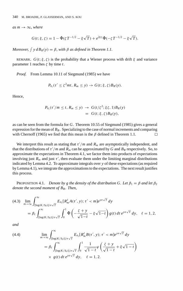
340 M. BROADIE, P. GLASSERMAN, AND S. KOU
as m→∞, where
G(t; ξ, ζ ) = 1−Φ(ζT−1/2− ξ√
T)+ e2ξζΦ(−ζT−1/2− ξ√
T).
Moreover,∫
y d BR(y) = β, withβ as defined in Theorem 1.1.
REMARK. G(t; ξ, ζ ) is the probability that a Wiener process with driftξ and varianceparameter 1 reachesζ by timet .
Proof. From Lemma 10.11 of Siegmund (1985) we have
Pθ1(τ′ ≤ ζ 2mt, Rm ≤ y)→ G(t; ξ, ζ )BR(y).
Hence,
Pθ1(τ′/m≤ t, Rm ≤ y) → G(t/ζ 2; ξζ, 1)BR(y)
= G(t; ξ, ζ )BR(y),
as can be seen from the formula forG. Theorem 10.55 of Siegmund (1985) gives a generalexpression for the mean ofBR. Specializing to the case of normal increments and comparingwith Chernoff (1965) we find that this mean is theβ defined in Theorem 1.1.
We interpret this result as stating thatτ ′/m andRm are asymptotically independent, andthat the distributions ofτ ′/m andRm can be approximated byG andBR respectively. So, toapproximate the expectations in Theorem 4.1, we factor them into products of expectationsinvolving just Rm and justτ ′, then evaluate them under the limiting marginal distributionsindicated by Lemma 4.2. To approximate integrals overy of these expectations (as requiredby Lemma 4.1), we integrate the approximations to the expectations. The next result justifiesthis process.
PROPOSITION4.1. Denote by g the density of the distribution G. Letβ1 = β and letβ2
denote the second moment of BR. Then,
limm→∞
∫ ∞[log(K/S0)]/σ
√T
Eθ1[R`mA(τ ′, y); τ ′ < m]eyσ
√T dy(4.3)
= β`∫ ∞
[log(K/S0)]/σ√
T
∫ 1
0Φ(− ζ + y√
1−t− ξ√1−t
)g(t) dt eyσ
√T dy, ` = 1, 2,
and
limm→∞
∫ ∞[log(K/S0)]/σ
√T
Eθ1[R`mB(τ ′, y); τ ′ < m]eyσ
√T dy(4.4)
= β`∫ ∞
[log(K/S0)]/σ√
T
∫ 1
0
1√1− t
ϕ
(ζ + y√1− t
+ ξ√1− t
)× g(t) dt eyσ
√T dy, ` = 1, 2.

A CONTINUITY CORRECTION FOR DISCRETE BARRIER OPTIONS 341
Proof. See Appendix B.
To evaluate the limits in Proposition 4.1, we need the following identities:
LEMMA 4.3.
∫ 1
0Φ(− x√
1− t− ξ√1− t
)g(t) dt = e2ξζΦ(−x − ζ − ξ).(4.5)
∫ 1
0
1√1− t
ϕ
(x√
1− t+ ξ√1− t
)g(t) dt = e2ξζ ϕ(x + ζ + ξ).(4.6)
Proof. Both identities can in principle be verified algebraically using the fact that
g(t) = ζ√2π
t−3/2 exp
{ξζ − 1
2
(ζ 2
t + ξ2t
)}, t > 0.
An alternative probabilistic argument notes that both sides of (4.5) are equal toP(τ (ξ) <1,W(ξ)
1 < ζ − x), whereW(ξ) is a unit-variance Wiener process with driftξ , andτ (ξ) is thefirst timeW(ξ) reachesζ . For the right side use equation (3.14) of Siegmund (1985) and forthe left side condition onτ . Both sides of (4.6) yield the corresponding density atζ − x.
Using Proposition 4.1 and Lemma 4.3, we can handle integrals of the first five expectationson the right side of equation (4.2) in Theorem 4.1. To dispense with integrals of the lasttwo expectations there, we need the following:
PROPOSITION4.2. For i = 1, 2,
lim supm→∞
Eθ1
[∫ ∞[log(K/S0)]/σ
√Tϕ′(ηi )
eyσ√
T
√1− τ ′/m
dy; τ ′ < m
]<∞,
whereη1, η2 are as in Theorem 4.1.
Proof. See Appendix C.
4.4. Comparison with the Continuous Price
Consider the expression given for the discrete price in Lemma 4.1. For the integrandappearing there, substitute the expression in (4.2) using the parameters in (4.1). Theorem 4.1applies because for anyy ≥ log(K/S0)/σ
√T we havey > log(H/S0)/σ
√T = −ζ . The

342 M. BROADIE, P. GLASSERMAN, AND S. KOU
result of the substitution is of the form
erT Vm(S0ea) =∫ ∞
[log(K/S0)]/σ√
Te2µa/σ 2
(1−Φ(y− 2a
σ√
T− µ√
T
σ
))× σ√
T S0eyσ√
T dy
+ 1√m
∫ ∞[log(K/S0)]/σ
√T
2Eθ1[Rm(ξ A(τ ′, u)− B(τ ′, y)); τ ′ < m]
× σ√
T S0eyσ√
T dy
+ 1
m
∫· · · dy
+ 1
m√
m
∫· · · dy.
Now apply (3.3) to the first integral, and invoke the boundedness of the limits in Proposi-tion 4.1 for` = 2 and the boundedness proved in Proposition 4.2 to write this as
erT Vm(S0ea) = erT V(S0ea)
+ 1√m
∫ ∞[log(K/S0)]/σ
√T
2Eθ1[Rm(ξ A(τ ′, u)− B(τ ′, y)); τ ′ < m]
× σ√
T S0eyσ√
T dy+ o
(1√m
).
We may replace the remaining integral with its limit asm→∞ and preserve the validityof this expression. Using Proposition 4.1 with` = 1 and then Lemma 4.3, we thus obtain
Vm(S0ea) = V(S0ea)+ 2ξβσ√
T√m
e−rT∫ ∞
[log(K/S0)]/σ√
Te2ξζΦ(−2ζ − y− ξ)S0eyσ
√T dy
− 2βσ√
T√m
e−rT∫ ∞
[log(K/S0)]/σ√
Te2ξζ ϕ(2ζ + y+ ξ)S0eyσ
√T dy+ o
(1√m
).
Substituting forξ andζ as in (4.1), we get
Vm(S0ea) =
V(S0ea)− βσ√
T√m
2µ√
T
σe−rT
∫ ∞[log(K/S0)]/σ
√T
e2µa/σ 2
×(
1−Φ(y− µ√
T
σ− 2a
σ√
T
))S0eyσ
√T dy
− βσ√
T√m
2e−rT e2µa/σ 2∫ ∞
[log(K/S0)]/σ√
Tϕ
(y− µ
√T
σ− 2a
σ√
T
)S0eyσ
√T dy
+ o
(1√m
).

A CONTINUITY CORRECTION FOR DISCRETE BARRIER OPTIONS 343
Comparing this with Proposition 3.2, we may rewrite it as
Vm(S0ea) = V(S0ea)− βσ√
T√m
∂aV(S0ea)+ o
(1√m
),
which is to say that
Vm(S0ea) = V(S0ea−βσ√1t )+ o
(1√m
),
concluding the proof of Theorem 1.1.Notice that if we simply omit the integral from the expression in Lemma 4.1, we obtain
the price of a discretely monitored binary barrier option. Omitting the integral from (3.3)produces the price of the corresponding continuously monitored barrier option. The stepscarried out in proving Theorem 1.1 for the integrals apply equally well—indeed, with muchless effort—for the integrands. Thus, we have the following corollary.
COROLLARY 4.1. Theorem 1.1 holds for binary barrier options as well.
APPENDIX A: PROOF OF THEOREM 4.1
Directly from Siegmund and Yuh (1982, p. 244), we have
Pθ1(τ′ < m,Um < −y
√m) = e(θ1−θ0)bPθ0(Um ≥ (2ζ + y)
√m)
−Eθ1
[e−(θ1−θ0)Rm
× {1− Fθ0,m−τ ′(
√m(y+ ζ )− Rm)− Fθ1,m−τ ′(−
√m(y+ ζ )− Rm)
} ; τ ′ < m],
whereFθ,n is the distribution ofUn underPθ . Let us write this as
Pθ1(τ′ < m,Um < −y
√m) = X − Eθ1[Y; τ ′ < m].(A.1)
Then
X = e2ξζ
(1−Φ( (2ζ + y)
√m− θ0m√
m
))= e2ξζ (1−Φ(2ζ + y+ ξ)),
which is exactly the first term on the right side of equation (4.2) in Theorem 4.1.Next we analyzeY. By the definition ofUn, eachFθ,n is a normal distribution with mean
nθ and variancen. Thus,
Y = e−2ξRm/√
m
(1−Φ( (y+ ζ )√m− Rm + ξ(m− τ ′)/
√m√
m− τ ′))
−Φ(−(y+ ζ )√m− Rm − ξ(m− τ ′)/√m√m− τ ′
).

344 M. BROADIE, P. GLASSERMAN, AND S. KOU
Taylor expansion now gives
Y = e−2ξRm/√
m
[1−Φ( y+ ζ√
1− τ ′/m+ ξ
√1− τ ′/m
)
+ Rm√m− τ ′ ϕ
(y+ ζ√
1− τ ′/m+ ξ
√1− τ ′/m
)+ 1
2
R2m
m− τ ′ ϕ′(η1)
]
−[Φ(− y+ ζ√
1− τ ′/m− ξ
√1− τ ′/m
)
− Rm√m− τ ′ ϕ
(− y+ ζ√
1− τ ′/m− ξ
√1− τ ′/m
)
+ 1
2
R2m
m− τ ′ ϕ′(η2)
],
for someη1, η2 as stated in the theorem. BecauseΦ(−x) = 1−Φ(x) andϕ(−x) = ϕ(x),this becomes
Y = (e−2ξRm/√
m − 1)Φ(− y+ ζ√1− τ ′/m
− ξ√
1− τ ′/m
)
+ (e−2ξRm/√
m + 1)Rm√
m− τ ′ ϕ(
y+ ζ√1− τ ′/m
+ ξ√
1− τ ′/m
)
+ e−2ξRm/√
m R2m
m− τ ′1
2ϕ′(η1)− R2
m
m− τ ′1
2ϕ′(η2).
For anyx ≥ 0 there is ac with |c| ≤ 1, such thate−x = 1−x+cx2. We may thus introduceC andD as stated in the theorem to get
Y = (−2ξRm/√
m)Φ(− y+ ζ√1− τ ′/m
− ξ√
1− τ ′/m
)
+C · 4ξ2 R2m
mΦ(− y+ ζ√
1− τ ′/m− ξ
√1− τ ′/m
)
+ (2− 2ξRm/√
m)Rm√
m− τ ′ ϕ(
y+ ζ√1− τ ′/m
+ ξ√
1− τ ′/m
)
+ D · 4ξ2 R2m
m
Rm√m− τ ′ ϕ
(y+ ζ√
1− τ ′/m+ ξ
√1− τ ′/m
)
+ e−2ξRm/√
m R2m
m− τ ′1
2ϕ′(η1)− R2
m
m− τ ′1
2ϕ′(η2).

A CONTINUITY CORRECTION FOR DISCRETE BARRIER OPTIONS 345
With A(τ ′, y) andB(τ ′, y) as defined in the theorem, this becomes
Y = (−2ξRm/√
m)A(τ ′, y)+ C · 4ξ2 R2m
mA(τ ′, y)
+ (2− 2ξRm/√
m)Rm√
mB(τ ′, y)+ D · 4ξ2 R3
m
m√
mB(τ ′, y)
+ e−2ξRm/√
m R2m
m− τ ′1
2ϕ′(η1)− R2
m
m− τ ′1
2ϕ′(η2).
Grouping terms according to their denominators, we get
Y = −2ξRm√m
A(τ ′, y)+ 2Rm√m
B(τ ′, y)
+ 1
mC · 4ξ2R2
mA(τ ′, y)− 1
m2ξR2
mB(τ ′, y)
+ 1
m√
mD · 4ξ2R2
mB(τ ′, y)
+ e−2ξRm/√
m R2m
m− τ ′1
2ϕ′(η1)− R2
m
m− τ ′1
2ϕ′(η2).
Via (A.1), this concludes the proof of the theorem.
APPENDIX B: UNIFORM INTEGRABILITY
The main objective of this appendix is to prove Proposition 4.1. We begin by recording twouseful facts. From Lemma 10.11 of Siegmund (1985) we get convergence of all momentsof the overshoot to moments ofBR:
limm→∞ Eθ1[R
qm] =
∫yqd BR(y), for all q > 0.(B.1)
In particular,Eθ1[Rm] → β. We will also use the easily verified identity
∫ ∞b
ecyϕ(u+ y) dy= ec(c+2u)/2Φ(−b+ c+ u).(B.2)
We now prove
LEMMA B.1. There is a finite constant M such that for all m
sup0≤t<m
∫ ∞[log(K/S0)]/σ
√T
B(t, y)eyσ√
T dy≤ M.

346 M. BROADIE, P. GLASSERMAN, AND S. KOU
Proof. Using first the definition ofB(t, y) and then (B.2), we get
∫ ∞[log(K/S0)]/σ
√T
B(t, y)eyσ√
T dy
=∫ ∞
[log(K/S0)]/σ√
Tϕ
(ζ + y√1− t/m
+ ξ√
1− t/m
)eyσ√
T dy√1− t/m
= exp
(1
2σ√
T√
1− t/m
[σ√
T√
1− t/m+ 2ξ√
1− t/m+ 2ζ√1− t/m
])×Φ(− log(K/S0)
σ√
T√
1− t/m+ σ√
T√
1− t/m+ ξ√
1− t/m+ ζ√1− t/m
),
and this is bounded for 0≤ t < m.
We proceed with the proof of Proposition 4.1, first considering (4.4). Because all quanti-ties inside the integral and expectation on the left side of (4.4) are nonnegative, by Tonelli’sTheorem we may interchange the integral and expectation to get
∫ ∞[log(K/S0)]/σ
√T
Eθ1[R`mB(τ ′, y); τ ′ < m]eyσ
√T dy
= Eθ1
[R`m
∫ ∞[log(K/S0)]/σ
√T
B(τ ′, y)eyσ√
T dy; τ ′ < m
].
By Lemma B.1, the integral inside the expectation is uniformly bounded. But then by (B.1)the entire expression inside the expectation is uniformly integrable. To evaluate the limitasm→∞, we may therefore integrate with respect to the limiting distribution to get
β`
∫ 1
0
∫ ∞[log(K/S0)]/σ
√T
1√1− t
ϕ
(ζ + y√1− t
+ ξ√1− t
)eyσ√
T dy g(t) dt.
Again interchanging the order of integration yields (4.4).The proof of (4.3) is similar. Just as in Lemma B.1, we integrate to verify that
∫ ∞[log(K/S0)]/σ
√T
A(t, y)eyσ√
T dy
is uniformly bounded for 0≤ t < m. This proves uniform integrability which, togetherwith two applications of Tonelli’s Theorem yields (4.3).
APPENDIX C: PROOF OF PROPOSITION 4.2
We begin with the following bound on the integral inside the expectation:

A CONTINUITY CORRECTION FOR DISCRETE BARRIER OPTIONS 347
LEMMA C.1. There are finite constants M1, M2, and M3 for which
sup0≤t<m
∣∣∣∣∣∫ ∞
[log(K/S0)]/σ√
Tϕ′(ηi )
eyσ√
T
√1− t/m
dy
∣∣∣∣∣ ≤ M1+ M2eM3Rm/√
m
for i = 1, 2.
Proof. For anyν > 0, integration by parts shows that
∫ ∞b
ecyϕ′(u+νy) dy= −1
νecbϕ(u+νb)− c
ν2exp
(1
2
c
ν
( c
ν+ 2u
))Φ (−νb+ c
ν+ u
).
Apply this identity to the integral in the lemma by settingb = log(K/S0)/(σ√
T), c =σ√
T , ν = 1/√
1− t/m, andu = ζ(1− t/m)−1/2+ ξ√1− t/m+ di , i = 1, 2, with
d1 ∈[− Rm√
m√
1− t/m, 0
]
d2 ∈[0,
Rm√m√
1− t/m
].
This results in a bound of the form in the lemma.
The proof of Proposition 4.2 will be complete once we verify that
lim supEθ1[exp(M3Rm/√
m)]
is finite asm→∞. For this we need
LEMMA C.2. There is a finite constant M4 such that Pθ1(Rm > u) ≤ M4e−u, for all mand all u≥ 0.
Proof. Since 1−Φ(x) ≤ 1x e−x2/2 ≤ e−x for all x > 0, by the argument of Example 2.2
on p. 19 of Woodroofe (1982) we have
Pθ1(Rm > u) =∞∑
n=1
Pθ1(τ′ ≥ n,Un > b+ u)
≤∞∑
n=1
Eθ1[e−(b+u−Un−1); τ ′ ≥ n]
= e−u∞∑
n=1
Eθ1[e−(b−Un−1); τ ′ ≥ n]
≡ M4e−u.

348 M. BROADIE, P. GLASSERMAN, AND S. KOU
It follows now that
Eθ1[eM3Rm/
√m] ≤ M4
∫ ∞0
eM3r/√
me−r dr,
which remains bounded asm→∞.
REFERENCES
AITSAHLIA , F. (1995): “Optimal Stopping and Weak Convergence Methods for Some Problemsin Financial Economics,” Doctoral dissertation, Department of Operations Research, StanfordUniversity, Stanford, CA.
ASMUSSEN, S. (1989): “Risk Theory in a Markovian Environment,”Scand. Actuarial J., 16, 69–100.
BLACK, F., and M. SCHOLES(1973): “The Pricing of Options and Corporate Liabilities,”J. PoliticalEconomy, 81, 637–659.
BOYLE, P. P., and S. H. LAU (1994): “Bumping Up Against the Barrier with the Binomial Method,”J. Derivatives,2, 6–14.
BROADIE, M., P. GLASSERMAN, and S. KOU (1996): “Connecting Discrete and Continuous Path-Dependent Options,” working paper, Columbia Business School, New York, to appear inFinanceand Stochastics.
CHANCE, D. M. (1994): “The Pricing and Hedging of Limited Exercise Caps and Spreads,”J.Financial Res., 17, 561–584.
CHERNOFF, H. (1965): “Sequential Tests for the Mean of a Normal Distribution IV,”Ann. Math.Statist., 36, 55–68.
CHERNOFF, H., and A. J. PETKAU (1986): “Numerical Solutions for Bayes Sequential DecisionProblems,”SIAM J. Sci. Stat. Comput., 7, 46–59.
Derivatives Week(1995a): “Discrete Path-Dependent Options,” April 10, 7.
Derivatives Week(1995b): “Liquidity Standards to be Drawn up for Barrier Options,” May 29, 2.
FLESAKER, B. (1992): “The Design and Valuation of Capped Stock Index Options,” working paper,Department of Finance, University of Illinois, Champaign, IL.
HEYNEN, R. C., and H. M. KAT (1994a): “Crossing Barriers,”RISK, 7 (June), 46–49. Correction(1995),RISK, 8, (March) 18.
HEYNEN, R. C., and H. M. KAT (1994b): “Partial Barrier Options,”J. Financial Engineering, 3(September/December), 253–274.
KARATZAS, I., and S. SHREVE (1991): Brownian Motion and Stochastic Calculus. New York:Springer-Verlag.
KAT, H., and L. VERDONK (1995): “Tree Surgery,”RISK, 8 (February), 53–56.
KUNITOMO, N., and M. IKEDA (1992): “Pricing Options with Curved Boundaries,”Math. Finance,2,275–298.
MERTON, R. C. (1973): “Theory of Rational Option Pricing,”Bell J. Econ. Mgmt. Sci., 4, 141–183.
RICH, D. (1994): “The Mathematical Foundations of Barrier Option Pricing Theory,”Adv. FuturesOpt. Res., 7, 267–312.
RICH, D. (1996): “The Valuation of Black-Scholes Options Subject to Intertemporal Default Risk,”Rev. Derivatives Res., 1, 25–59.
RUBINSTEIN, M., and E. REINER(1991): “Breaking Down the Barriers,”RISK, 4 (September), 28–35.
SIEGMUND, D. (1979): “Corrected Diffusion Approximations in Certain Random Walk Problems,”Adv. Appl. Probab., 11, 701–719.

A CONTINUITY CORRECTION FOR DISCRETE BARRIER OPTIONS 349
SIEGMUND, D. (1985): Sequential Analysis: Tests and Confidence Intervals. New York: Springer-Verlag.
SIEGMUND, D., and Y.-S. YUH (1982): “Brownian Approximations for First Passage Probabilities,”Z. Wahrsch. verw. Gebiete,59, 239–248.
WOODROOFE, M. (1982): Nonlinear Renewal Theory in Sequential Analysis. Philadelphia: Societyfor Industrial and Applied Mathematics.