Module 2: Introduction to Statistics - bioboot.github.io · Pearson's Chi‐squared test with...
28
3/3/2015 1 Module 2: Introduction to Statistics Niko Kaciroti, Ph.D. BIOINF 525 Module 2: W15 University of Michigan Topic • Dichotomous Variables • Compare Proportions – Two sample test (Normal approximation theory) – Chi‐square test – Fisher Exact test • Measuring Treatment Effect on Binary Outcomes – Absolute Risk Reduction (ARR) – Relative Risk (RR) – Odds Ratio (OR) • Application and Discussion of a Research Article – Feasibility of treating prehypertension with an angiotensin‐receptor blocker. Julius S. et al. N Engl J Med. 2006; 354:1685‐97
Transcript of Module 2: Introduction to Statistics - bioboot.github.io · Pearson's Chi‐squared test with...
3/3/2015
1
Module 2: Introduction to Statistics
Niko Kaciroti, Ph.D.BIOINF 525 Module 2: W15University of Michigan
Topic
• Dichotomous Variables
• Compare Proportions
– Two sample test (Normal approximation theory)
– Chi‐square test
– Fisher Exact test
• Measuring Treatment Effect on Binary Outcomes
– Absolute Risk Reduction (ARR)
– Relative Risk (RR)
– Odds Ratio (OR)
• Application and Discussion of a Research Article
– Feasibility of treating prehypertension with an angiotensin‐receptor blocker. Julius S. et al. N Engl J Med. 2006; 354:1685‐97
3/3/2015
2
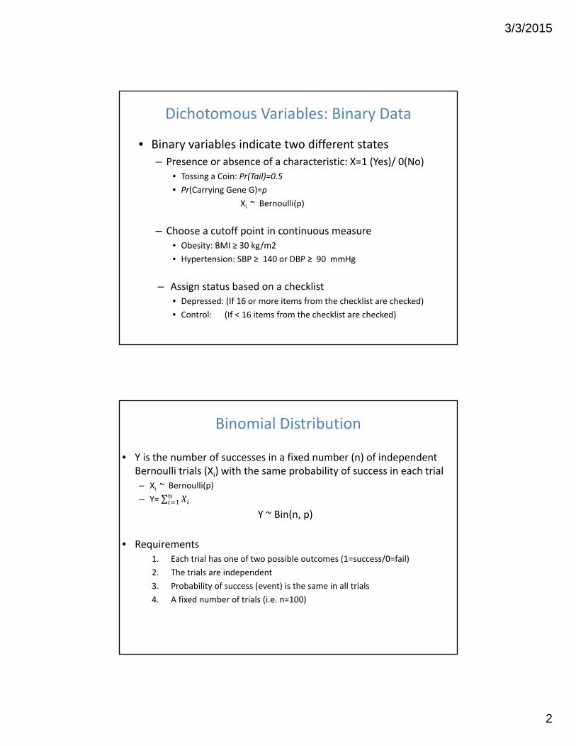
Dichotomous Variables: Binary Data
• Binary variables indicate two different states
– Presence or absence of a characteristic: X=1 (Yes)/ 0(No)• Tossing a Coin: Pr(Tail)=0.5
• Pr(Carrying Gene G)=p
Xi ~ Bernoulli(p)
– Choose a cutoff point in continuous measure• Obesity: BMI ≥ 30 kg/m2
• Hypertension: SBP ≥ 140 or DBP ≥ 90 mmHg
– Assign status based on a checklist • Depressed: (If 16 or more items from the checklist are checked)
• Control: (If < 16 items from the checklist are checked)
Binomial Distribution
• Y is the number of successes in a fixed number (n) of independent Bernoulli trials (Xi) with the same probability of success in each trial– Xi ~ Bernoulli(p)
– Y= ∑
Y ~ Bin(n, p)
• Requirements1. Each trial has one of two possible outcomes (1=success/0=fail)
2. The trials are independent
3. Probability of success (event) is the same in all trials
4. A fixed number of trials (i.e. n=100)
3/3/2015
3
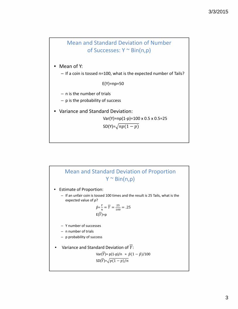
Mean and Standard Deviation of Number of Successes: Y ~ Bin(n,p)
• Mean of Y:
– If a coin is tossed n=100, what is the expected number of Tails?
E(Y)=np=50
– n is the number of trials
– p is the probability of success
• Variance and Standard Deviation:
Var(Y)=np(1‐p)=100 x 0.5 x 0.5=25
SD(Y)= 1
Mean and Standard Deviation of Proportion Y ~ Bin(n,p)
• Estimate of Proportion:– If an unfair coin is tossed 100 times and the result is 25 Tails, what is the
expected value of p?
= .25
E( )=p
– Y number of successes
– n number of trials
– p probability of success
• Variance and Standard Deviation of :
Var( )= p(1‐p)/n ≈ 1 /100
SD( )= 1 /
3/3/2015
4
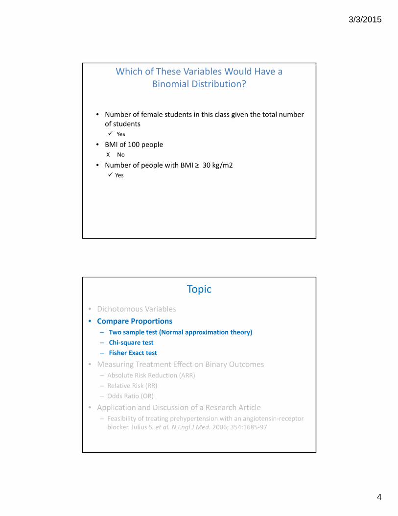
Which of These Variables Would Have a Binomial Distribution?
• Number of female students in this class given the total number of students Yes
• BMI of 100 peopleX No
• Number of people with BMI ≥ 30 kg/m2 Yes
Topic
• Dichotomous Variables
• Compare Proportions
– Two sample test (Normal approximation theory)
– Chi‐square test
– Fisher Exact test
• Measuring Treatment Effect on Binary Outcomes
– Absolute Risk Reduction (ARR)
– Relative Risk (RR)
– Odds Ratio (OR)
• Application and Discussion of a Research Article
– Feasibility of treating prehypertension with an angiotensin‐receptor blocker. Julius S. et al. N Engl J Med. 2006; 354:1685‐97
3/3/2015
5
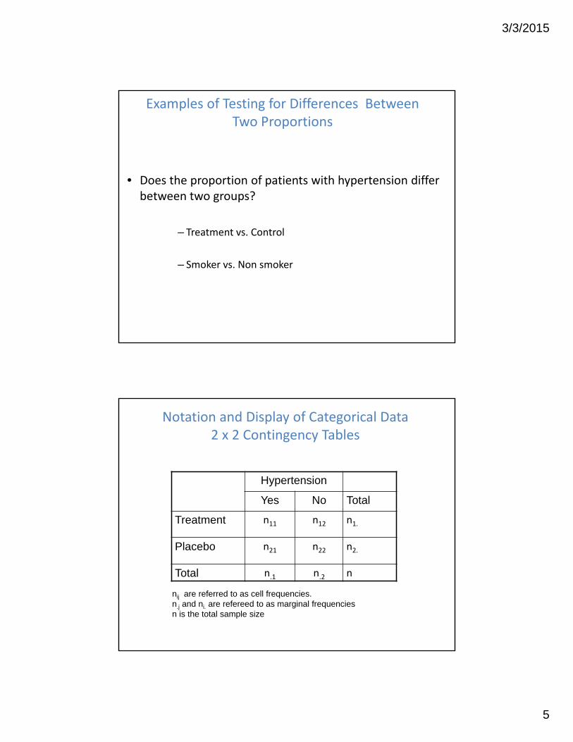
Examples of Testing for Differences Between Two Proportions
• Does the proportion of patients with hypertension differ between two groups?
– Treatment vs. Control
– Smoker vs. Non smoker
Notation and Display of Categorical Data2 x 2 Contingency Tables
Hypertension
Yes No Total
Treatment n11 n12 n1.
Placebo n21 n22 n2.
Total n.1 n.2 n
nij are referred to as cell frequencies. n.j and ni. are refereed to as marginal frequenciesn is the total sample size
3/3/2015
6
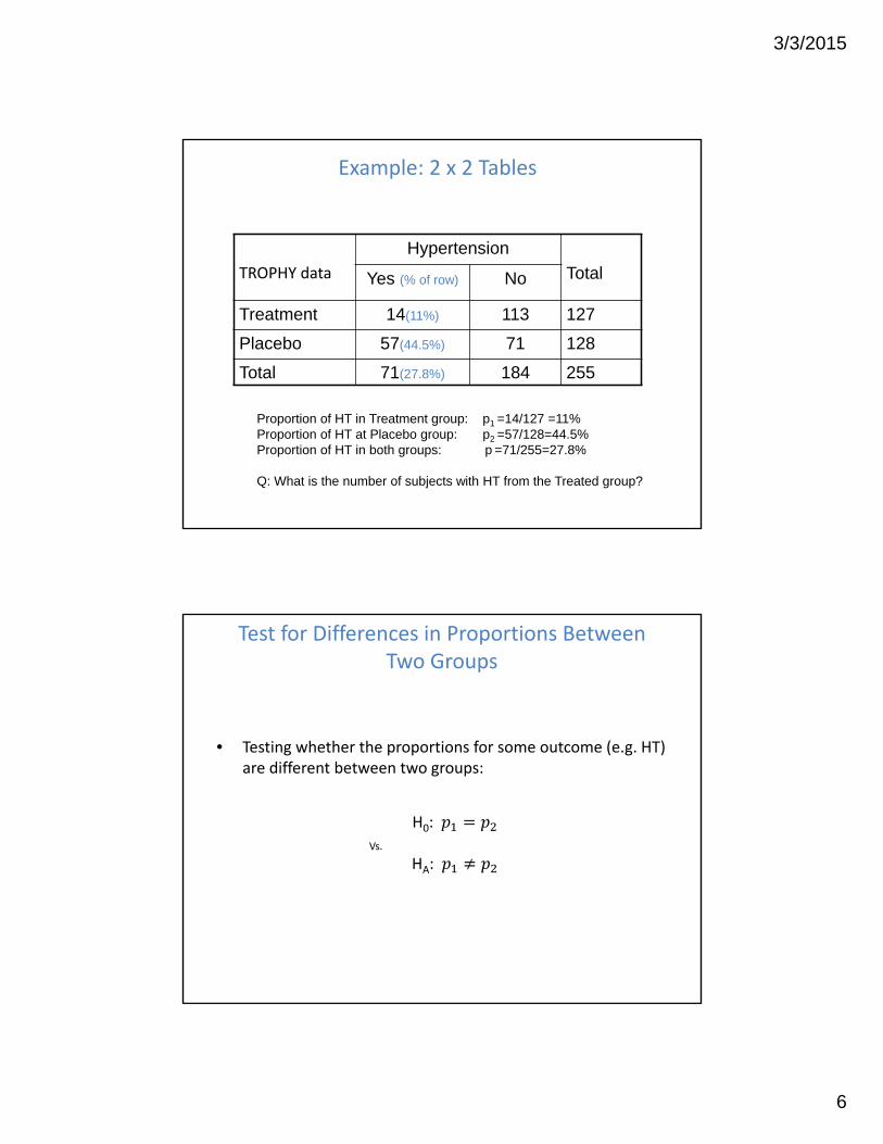
Example: 2 x 2 Tables
TROPHY data
Hypertension
TotalYes (% of row) No
Treatment 14(11%) 113 127
Placebo 57(44.5%) 71 128
Total 71(27.8%) 184 255
Proportion of HT in Treatment group: p1 =14/127 =11%Proportion of HT at Placebo group: p2 =57/128=44.5%Proportion of HT in both groups: p =71/255=27.8%
Q: What is the number of subjects with HT from the Treated group?
Test for Differences in Proportions Between Two Groups
• Testing whether the proportions for some outcome (e.g. HT) are different between two groups:
H0:
Vs.
HA:
3/3/2015
7
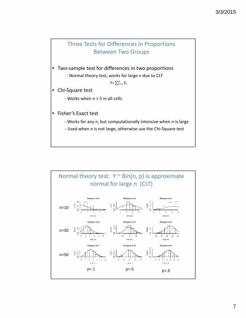
Three Tests for Differences in Proportions Between Two Groups
• Two‐sample test for differences in two proportions
‐ Normal theory test, works for large n due to CLT
Y= ∑
• Chi‐Square test
‐Works when n > 5 in all cells
• Fisher’s Exact test
‐Works for any n, but computationally intensive when n is large
‐ Used when n is not large, otherwise use the Chi‐Square test
Normal theory test: Y ~ Bin(n, p) is approximate normal for large n (CLT)
n=10
n=30
n=50
p=.1 p=.5 p=.9
3/3/2015
8
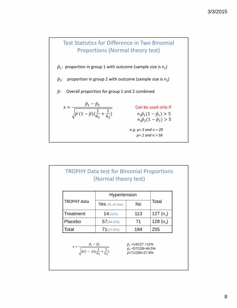
Test Statistics for Difference in Two Binomial Proportions (Normal theory test)
: proportion in group 1 with outcome (sample size is n1)
: proportion in group 2 with outcome (sample size is n2)
: Overall proportion for group 1 and 2 combined
Can be used only if
n1 1 5n2 1 5
e.g. p=.5 and n > 20
p=.1 and n > 56
z
1 1 1
TROPHY Data test for Binomial Proportions (Normal theory test)
TROPHY data
Hypertension
TotalYes (% of row) No
Treatment 14(11%) 113 127 (n1)
Placebo 57(44.5%) 71 128 (n2)
Total 71(27.8%) 184 255
=14/127 =11% =57/128=44.5%=71/255=27.8%
z
1 1 1
3/3/2015
9
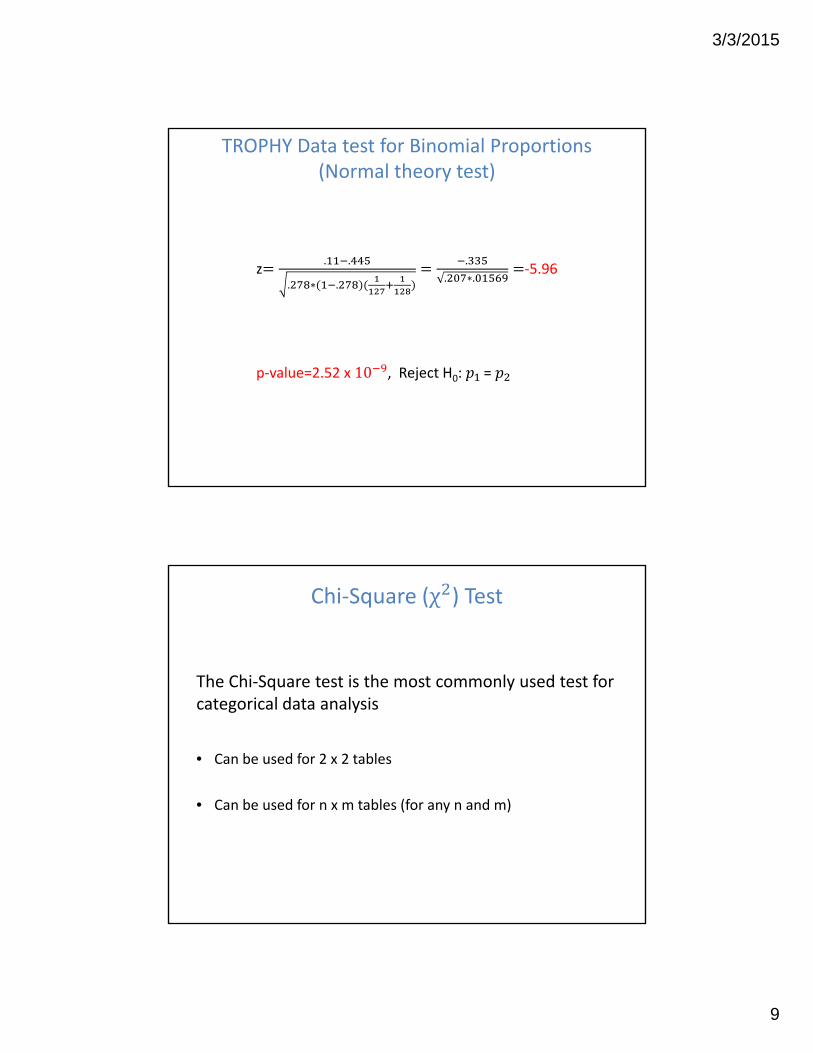
TROPHY Data test for Binomial Proportions (Normal theory test)
z. .
. ∗ .
.
. ∗.‐5.96
p‐value=2.52 x 10 , Reject H0: =
Chi‐Square (χ ) Test
The Chi‐Square test is the most commonly used test for categorical data analysis
• Can be used for 2 x 2 tables
• Can be used for n x m tables (for any n and m)
3/3/2015
10
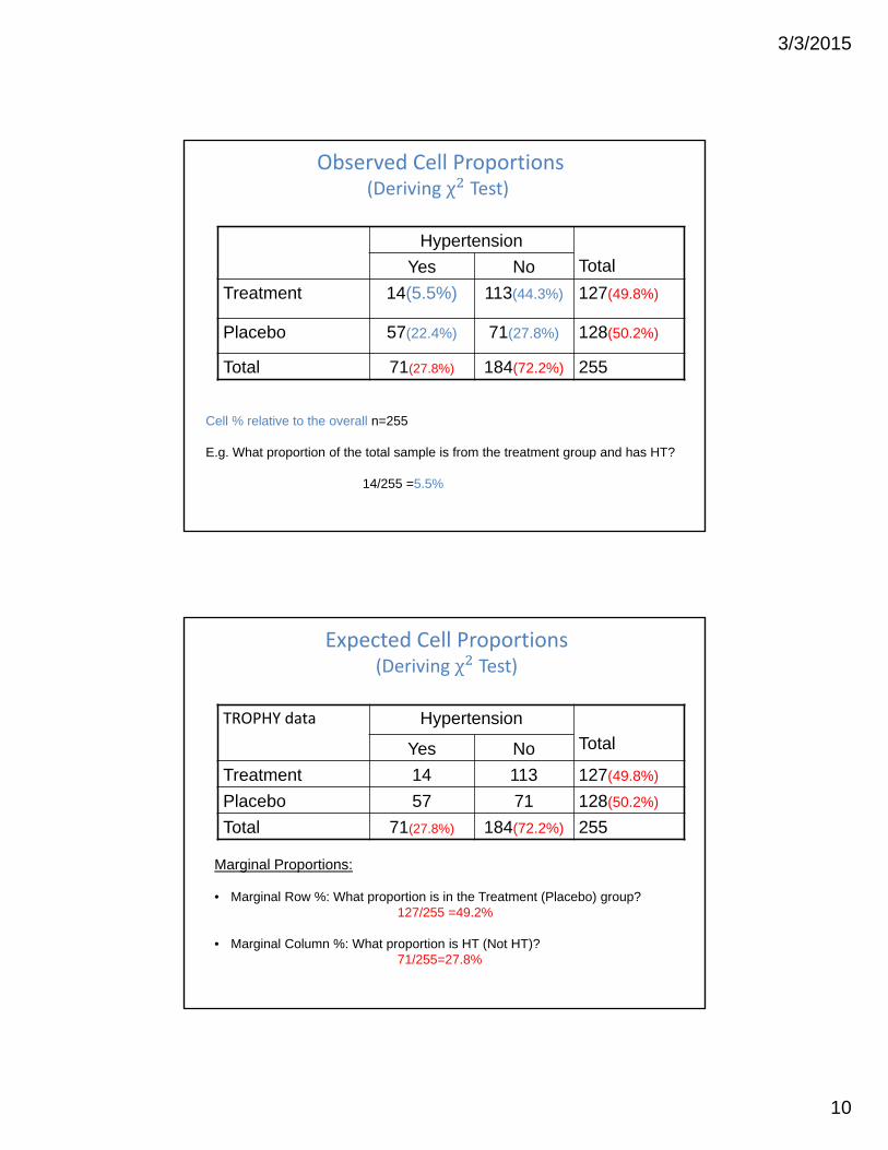
Observed Cell Proportions(Deriving χ Test)
Hypertension
TotalYes No
Treatment 14(5.5%) 113(44.3%) 127(49.8%)
Placebo 57(22.4%) 71(27.8%) 128(50.2%)
Total 71(27.8%) 184(72.2%) 255
Cell % relative to the overall n=255
E.g. What proportion of the total sample is from the treatment group and has HT?
14/255 =5.5%
Expected Cell Proportions (Deriving χ Test)
TROPHY data Hypertension
TotalYes No
Treatment 14 113 127(49.8%)
Placebo 57 71 128(50.2%)
Total 71(27.8%) 184(72.2%) 255
Marginal Proportions:
• Marginal Row %: What proportion is in the Treatment (Placebo) group?127/255 =49.2%
• Marginal Column %: What proportion is HT (Not HT)?71/255=27.8%
3/3/2015
11
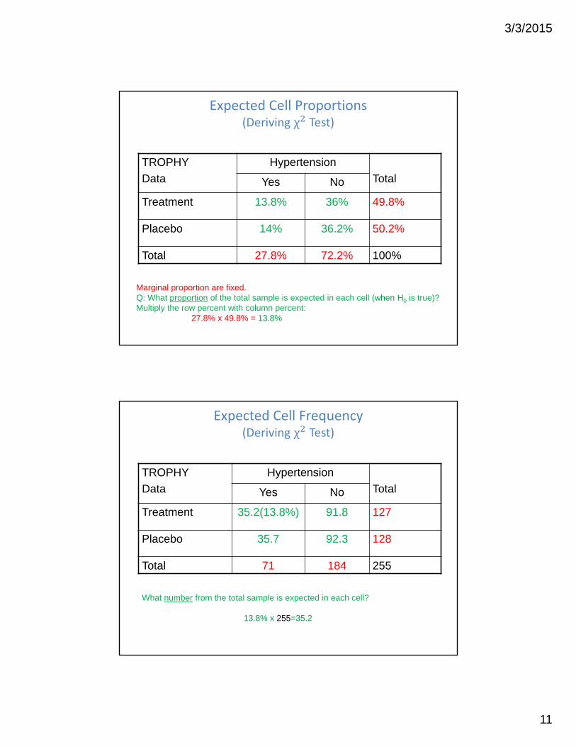
Expected Cell Proportions(Deriving χ Test)
TROPHY
Data
Hypertension
TotalYes No
Treatment 13.8% 36% 49.8%
Placebo 14% 36.2% 50.2%
Total 27.8% 72.2% 100%
Marginal proportion are fixed.Q: What proportion of the total sample is expected in each cell (when H0 is true)? Multiply the row percent with column percent:
27.8% x 49.8% = 13.8%
Expected Cell Frequency(Deriving χ Test)
TROPHY
Data
Hypertension
TotalYes No
Treatment 35.2(13.8%) 91.8 127
Placebo 35.7 92.3 128
Total 71 184 255
What number from the total sample is expected in each cell?
13.8% x 255=35.2
3/3/2015
12
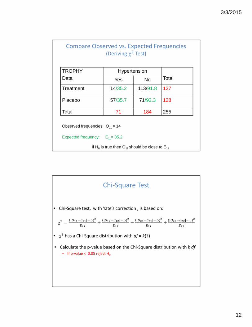
Compare Observed vs. Expected Frequencies(Deriving χ Test)
TROPHY
Data
Hypertension
TotalYes No
Treatment 14/35.2 113/91.8 127
Placebo 57/35.7 71/92.3 128
Total 71 184 255
Observed frequencies: O11 = 14
Expected frequency: E11= 35.2
If H0 is true then O11 should be close to E11
Chi‐Square Test
• Chi‐Square test, with Yate’s correction , is based on:
χ | | . | | . | | . | | .
• χ has a Chi‐Square distribution with df = k(?)
• Calculate the p‐value based on the Chi‐Square distribution with k df– If p‐value < 0.05 reject H0
3/3/2015
13
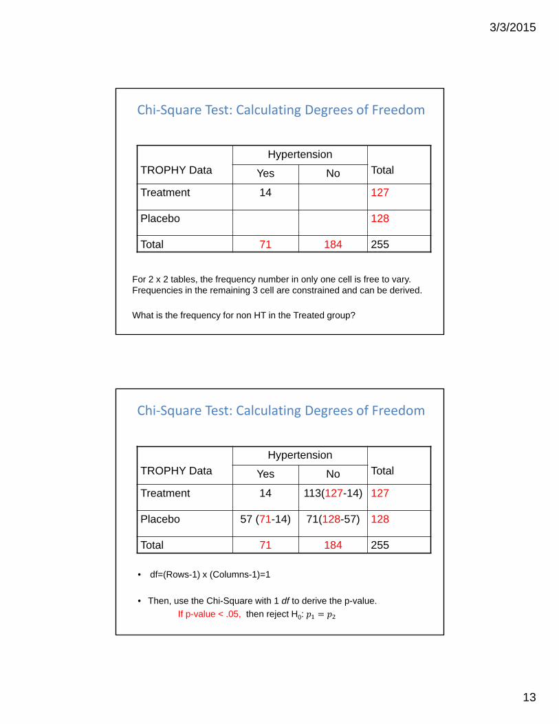
Chi‐Square Test: Calculating Degrees of Freedom
TROPHY Data
Hypertension
TotalYes No
Treatment 14 127
Placebo 128
Total 71 184 255
For 2 x 2 tables, the frequency number in only one cell is free to vary. Frequencies in the remaining 3 cell are constrained and can be derived.
What is the frequency for non HT in the Treated group?
Chi‐Square Test: Calculating Degrees of Freedom
TROPHY Data
Hypertension
TotalYes No
Treatment 14 113(127-14) 127
Placebo 57 (71-14) 71(128-57) 128
Total 71 184 255
• df=(Rows-1) x (Columns-1)=1
• Then, use the Chi-Square with 1 df to derive the p-value.
If p-value < .05, then reject H0:
3/3/2015
14
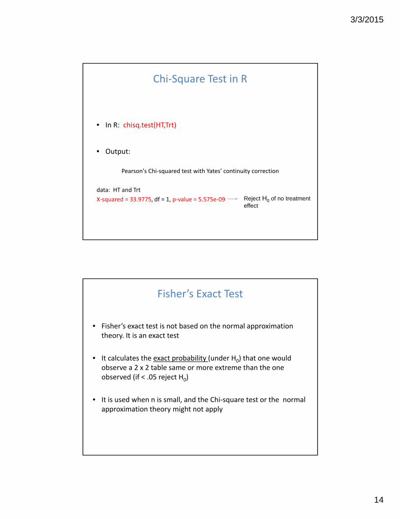
Chi‐Square Test in R
• In R: chisq.test(HT,Trt)
• Output:
Pearson's Chi‐squared test with Yates' continuity correction
data: HT and Trt
X‐squared = 33.9775, df = 1, p‐value = 5.575e‐09 Reject H0 of no treatment effect
Fisher’s Exact Test
• Fisher’s exact test is not based on the normal approximation theory. It is an exact test
• It calculates the exact probability (under H0) that one would observe a 2 x 2 table same or more extreme than the one observed (if < .05 reject H0)
• It is used when n is small, and the Chi‐square test or the normal approximation theory might not apply
3/3/2015
15
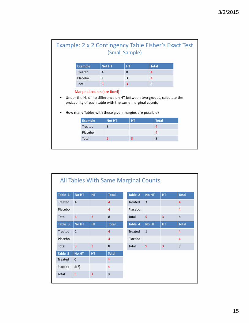
Example: 2 x 2 Contingency Table Fisher’s Exact Test (Small Sample)
Marginal counts (are fixed)
• Under the H0 of no difference on HT between two groups, calculate the probability of each table with the same marginal counts
• How many Tables with these given margins are possible?
Example Not HT HT Total
Treated 4 0 4
Placebo 1 3 4
Total 5 3 8
Example Not HT HT Total
Treated ? 4
Placebo 4
Total 5 3 8
All Tables With Same Marginal Counts
Table 2 No HT HT Total
Treated 3 4
Placebo 4
Total 5 3 8
Table 3 No HT HT Total
Treated 2 4
Placebo 4
Total 5 3 8
Table 1 No HT HT Total
Treated 4 4
Placebo 4
Total 5 3 8
Table 4 No HT HT Total
Treated 1 4
Placebo 4
Total 5 3 8
Table 5 No HT HT Total
Treated 0 4
Placebo 5(?) 4
Total 5 3 8
3/3/2015
16
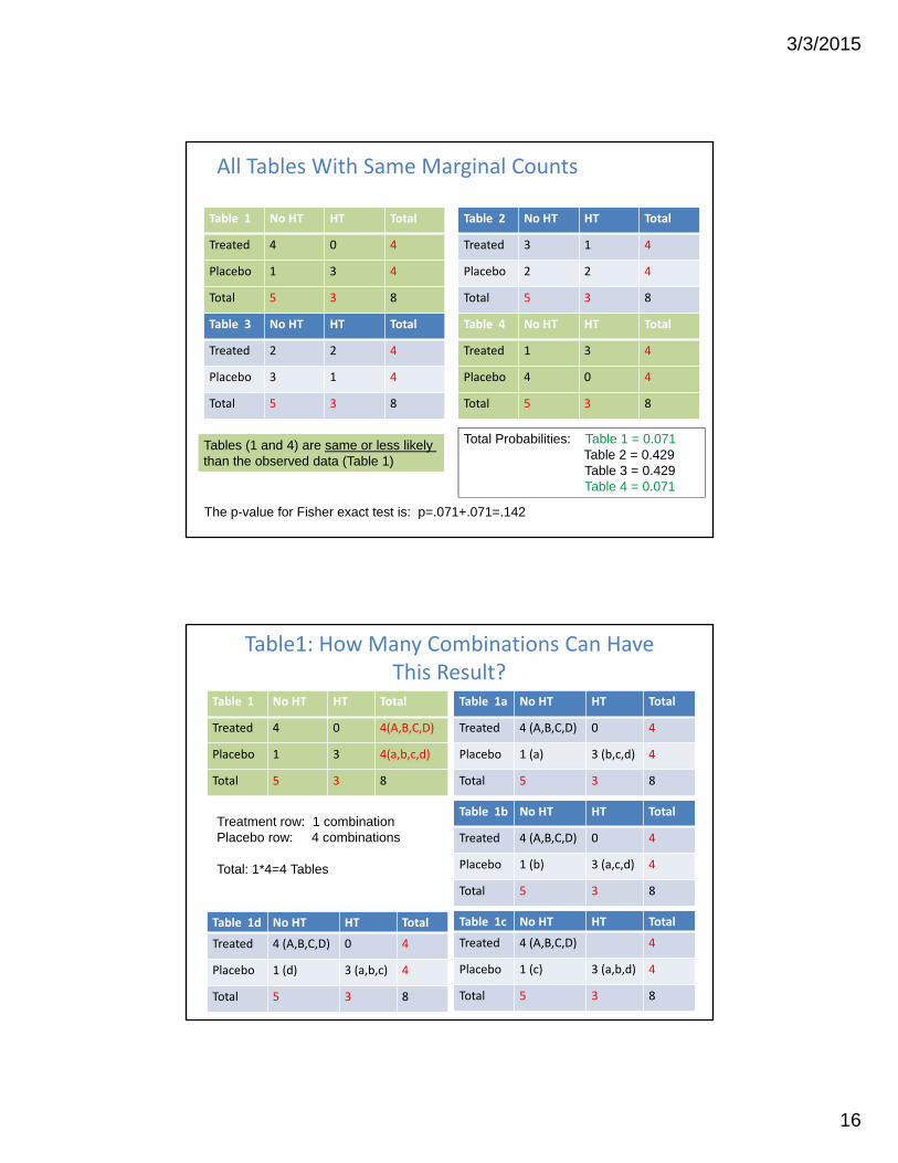
All Tables With Same Marginal Counts
Table 1 No HT HT Total
Treated 4 0 4
Placebo 1 3 4
Total 5 3 8
Table 2 No HT HT Total
Treated 3 1 4
Placebo 2 2 4
Total 5 3 8
Table 3 No HT HT Total
Treated 2 2 4
Placebo 3 1 4
Total 5 3 8
Table 4 No HT HT Total
Treated 1 3 4
Placebo 4 0 4
Total 5 3 8
Total Probabilities: Table 1 = 0.071 Table 2 = 0.429 Table 3 = 0.429 Table 4 = 0.071
Tables (1 and 4) are same or less likely than the observed data (Table 1)
The p-value for Fisher exact test is: p=.071+.071=.142
Table1: How Many Combinations Can Have This Result?
Table 1 No HT HT Total
Treated 4 0 4(A,B,C,D)
Placebo 1 3 4(a,b,c,d)
Total 5 3 8
Table 1a No HT HT Total
Treated 4 (A,B,C,D) 0 4
Placebo 1 (a) 3 (b,c,d) 4
Total 5 3 8
Table 1d No HT HT Total
Treated 4 (A,B,C,D) 0 4
Placebo 1 (d) 3 (a,b,c) 4
Total 5 3 8
Table 1c No HT HT Total
Treated 4 (A,B,C,D) 4
Placebo 1 (c) 3 (a,b,d) 4
Total 5 3 8
Table 1b No HT HT Total
Treated 4 (A,B,C,D) 0 4
Placebo 1 (b) 3 (a,c,d) 4
Total 5 3 8
Treatment row: 1 combinationPlacebo row: 4 combinations
Total: 1*4=4 Tables
3/3/2015
17
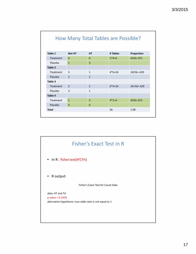
How Many Total Tables are Possible?
Table 1 Not HT HT # Tables Proportion
Treatment 4 0 1*4=4 4/56=.071
Placebo 1 3
Table 2
Treatment 3 1 4*6=24 24/56=.429
Placebo 2 2
Table 3
Treatment 2 2 6*4=24 24=56=.429
Placebo 3 1
Table 4
Treatment 1 3 4*1=4 4/56=.071
Placebo 4 0
Total 56 1.00
Fisher’s Exact Test in R
• In R: fisher.test(HT,Trt)
• R output:
Fisher's Exact Test for Count Data
data: HT and Trt
p‐value = 0.1429
alternative hypothesis: true odds ratio is not equal to 1
3/3/2015
18
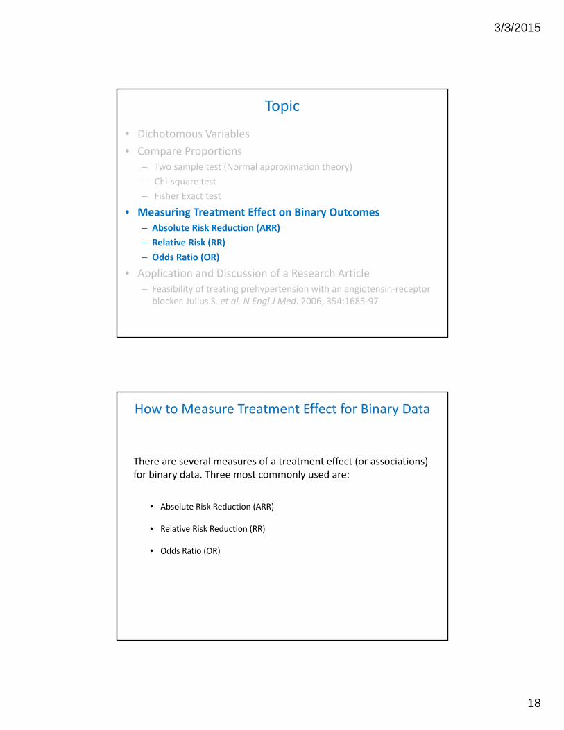
Topic
• Dichotomous Variables
• Compare Proportions
– Two sample test (Normal approximation theory)
– Chi‐square test
– Fisher Exact test
• Measuring Treatment Effect on Binary Outcomes
– Absolute Risk Reduction (ARR)
– Relative Risk (RR)
– Odds Ratio (OR)
• Application and Discussion of a Research Article
– Feasibility of treating prehypertension with an angiotensin‐receptor blocker. Julius S. et al. N Engl J Med. 2006; 354:1685‐97
How to Measure Treatment Effect for Binary Data
There are several measures of a treatment effect (or associations) for binary data. Three most commonly used are:
• Absolute Risk Reduction (ARR)
• Relative Risk Reduction (RR)
• Odds Ratio (OR)
3/3/2015
19
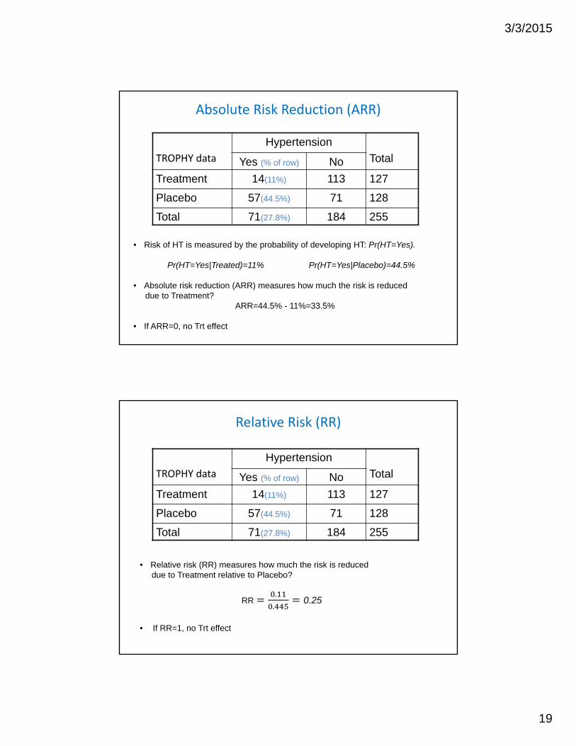
Absolute Risk Reduction (ARR)
TROPHY data
Hypertension
TotalYes (% of row) No
Treatment 14(11%) 113 127
Placebo 57(44.5%) 71 128
Total 71(27.8%) 184 255
• Risk of HT is measured by the probability of developing HT: Pr(HT=Yes).
Pr(HT=Yes|Treated)=11% Pr(HT=Yes|Placebo)=44.5%
• Absolute risk reduction (ARR) measures how much the risk is reduceddue to Treatment?
ARR=44.5% - 11%=33.5%
• If ARR=0, no Trt effect
Relative Risk (RR)
TROPHY data
Hypertension
TotalYes (% of row) No
Treatment 14(11%) 113 127
Placebo 57(44.5%) 71 128
Total 71(27.8%) 184 255
• Relative risk (RR) measures how much the risk is reduced due to Treatment relative to Placebo?
RR.
.0.25
• If RR=1, no Trt effect
3/3/2015
20
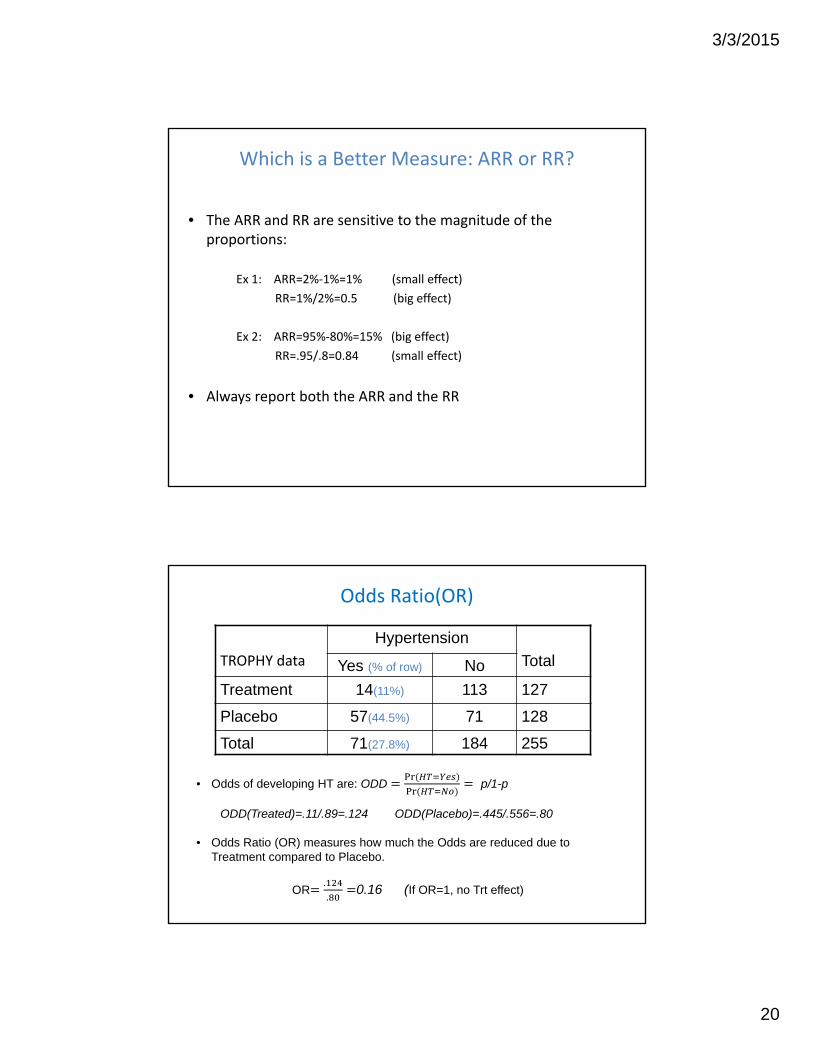
Which is a Better Measure: ARR or RR?
• The ARR and RR are sensitive to the magnitude of the proportions:
Ex 1: ARR=2%‐1%=1% (small effect)
RR=1%/2%=0.5 (big effect)
Ex 2: ARR=95%‐80%=15% (big effect)
RR=.95/.8=0.84 (small effect)
• Always report both the ARR and the RR
Odds Ratio(OR)
TROPHY data
Hypertension
TotalYes (% of row) No
Treatment 14(11%) 113 127
Placebo 57(44.5%) 71 128
Total 71(27.8%) 184 255
• Odds of developing HT are: ODD p/1-p
ODD(Treated)=.11/.89=.124 ODD(Placebo)=.445/.556=.80
• Odds Ratio (OR) measures how much the Odds are reduced due to Treatment compared to Placebo.
OR.
.0.16 (If OR=1, no Trt effect)
3/3/2015
21
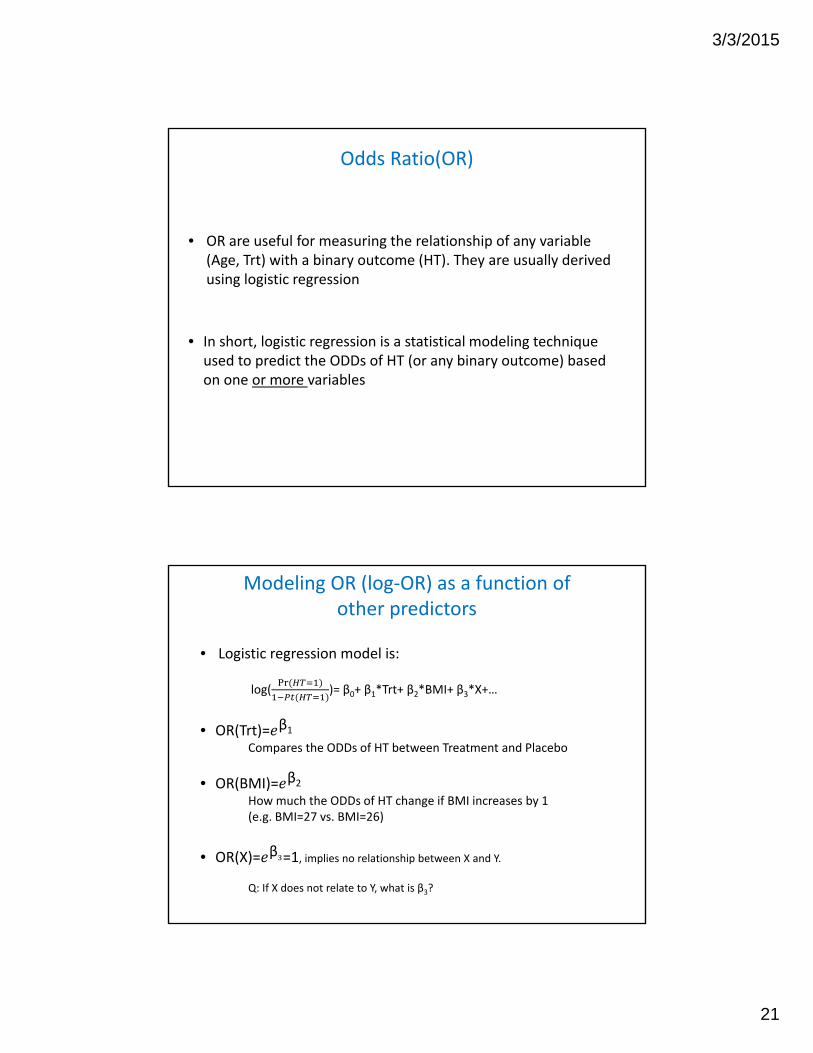
Odds Ratio(OR)
• OR are useful for measuring the relationship of any variable (Age, Trt) with a binary outcome (HT). They are usually derived using logistic regression
• In short, logistic regression is a statistical modeling technique used to predict the ODDs of HT (or any binary outcome) based on one or more variables
Modeling OR (log‐OR) as a function ofother predictors
• Logistic regression model is:
log( )= β0+ β1*Trt+ β2*BMI+ β3*X+…
• OR(Trt)= β1Compares the ODDs of HT between Treatment and Placebo
• OR(BMI)= β2How much the ODDs of HT change if BMI increases by 1(e.g. BMI=27 vs. BMI=26)
• OR(X)= β =1, implies no relationship between X and Y.
Q: If X does not relate to Y, what is β3?
3/3/2015
22
Topic
• Dichotomous Variables
• Compare Proportions
– Two sample test (Normal approximation theory)
– Chi‐square test
– Fisher Exact test
• Measuring Treatment Effect on Binary Outcomes
– Absolute Risk Reduction (ARR)
– Relative Risk (RR)
– Odds Ratio (OR)
• Application and Discussion of a Research Article
– Feasibility of treating prehypertension with an angiotensin‐receptor blocker. Julius S. et al. N Engl J Med. 2006; 354:1685‐97
Application and Discussion of a Research Article*
• Trial of Preventing Hypertension (TROPHY Study)
– Background: Hypertension is a strong predictor of excessive cardiovascular risk. TROPHY study investigated whether pharmacologic treatment of prehypertension prevents or postpones hypertension, thus reducing the CV risk.
*Feasibility of treating prehypertension with an angiotensin‐receptor blocker.
Julius S. et. al. N Engl J Med. 2006; 354:1685‐97
3/3/2015
23
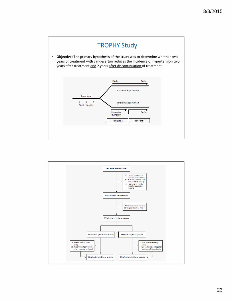
TROPHY Study
• Objective: The primary hypothesis of the study was to determine whether two years of treatment with candesartan reduces the incidence of hypertension two years after treatment and 2 years after discontinuation of treatment.
3/3/2015
24
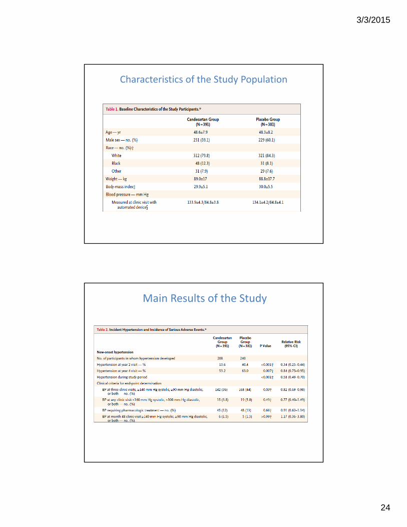
Characteristics of the Study Population
Main Results of the Study
3/3/2015
25
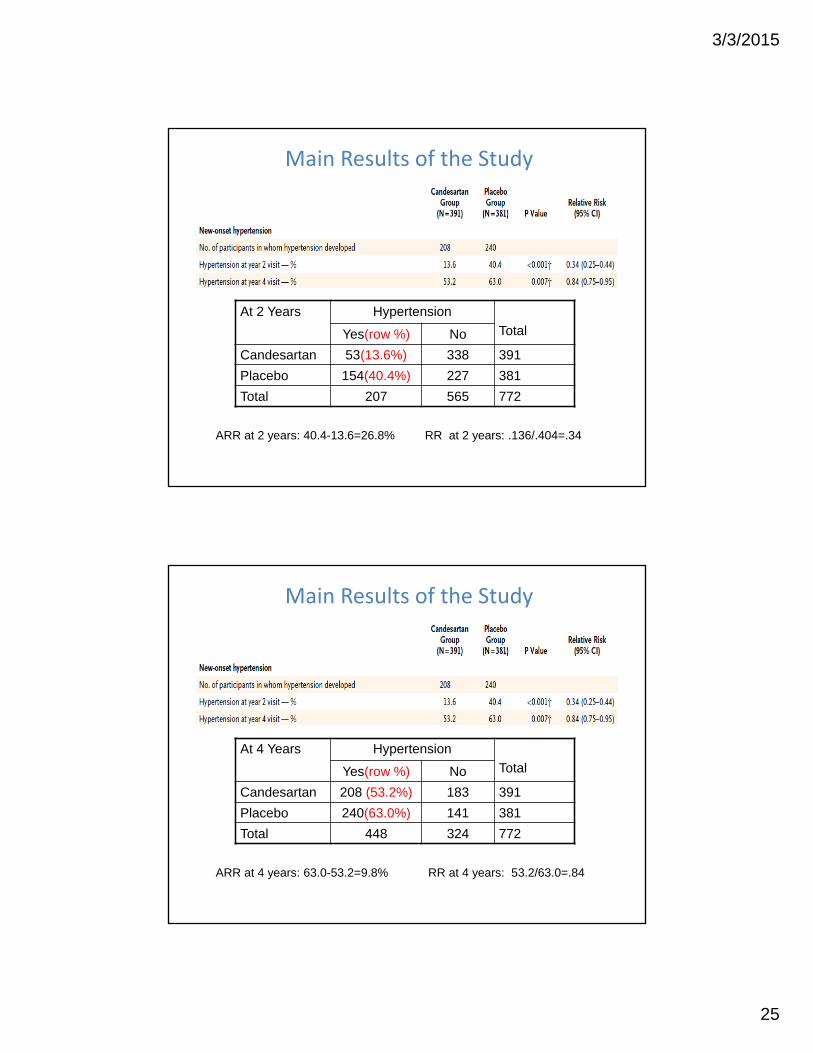
Main Results of the Study
ARR at 2 years: 40.4-13.6=26.8% RR at 2 years: .136/.404=.34
At 2 Years Hypertension
TotalYes(row %) No
Candesartan 53(13.6%) 338 391
Placebo 154(40.4%) 227 381
Total 207 565 772
Main Results of the Study
ARR at 4 years: 63.0-53.2=9.8% RR at 4 years: 53.2/63.0=.84
At 4 Years Hypertension
TotalYes(row %) No
Candesartan 208 (53.2%) 183 391
Placebo 240(63.0%) 141 381
Total 448 324 772
3/3/2015
26
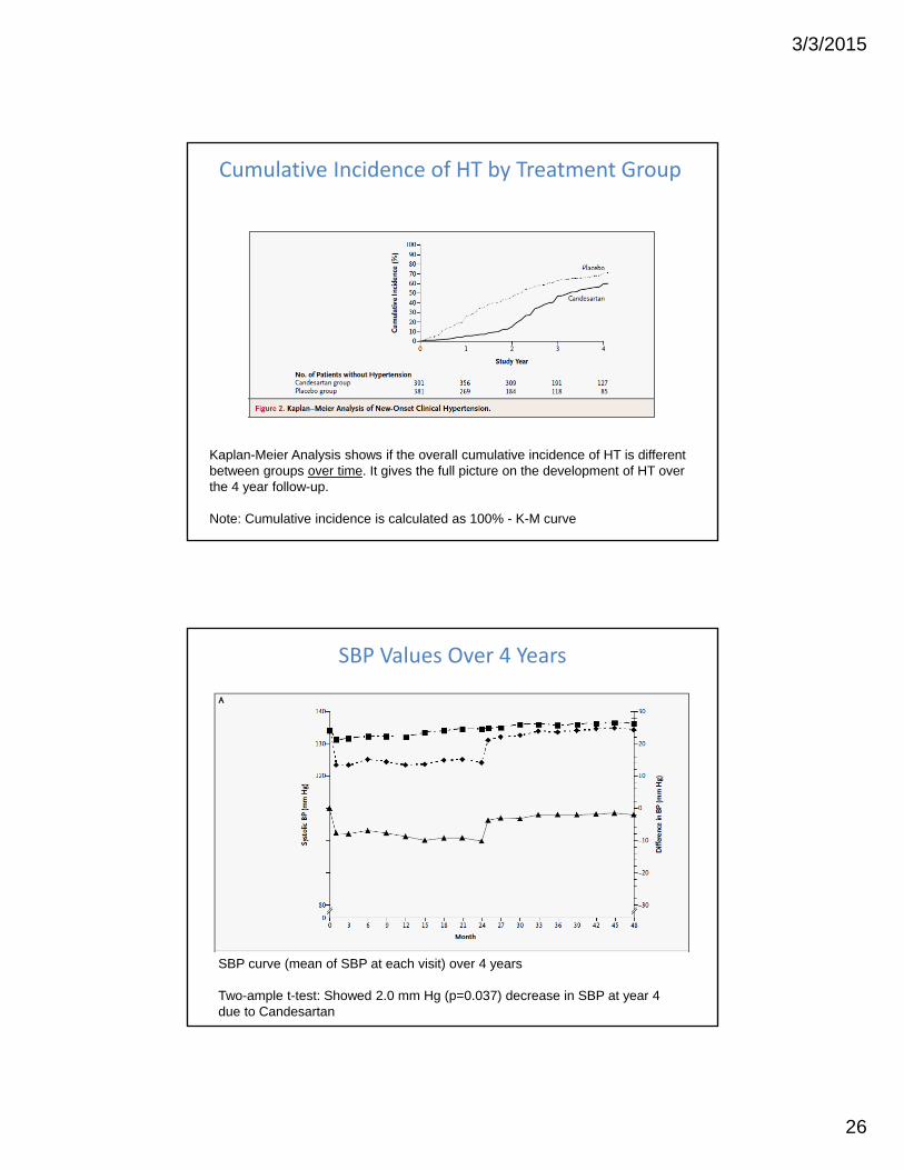
Cumulative Incidence of HT by Treatment Group
Kaplan-Meier Analysis shows if the overall cumulative incidence of HT is different between groups over time. It gives the full picture on the development of HT over the 4 year follow-up.
Note: Cumulative incidence is calculated as 100% - K-M curve
SBP Values Over 4 Years
SBP curve (mean of SBP at each visit) over 4 years
Two-ample t-test: Showed 2.0 mm Hg (p=0.037) decrease in SBP at year 4 due to Candesartan
3/3/2015
27
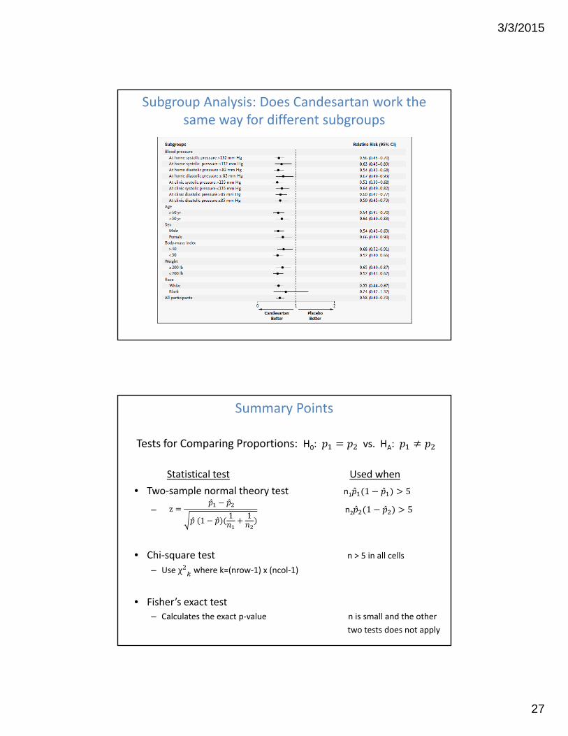
Subgroup Analysis: Does Candesartan work the same way for different subgroups
Summary Points
Tests for Comparing Proportions: H0: vs. HA:
Statistical test Used when
• Two‐sample normal theory test n1 1 5
– n2 1 5
• Chi‐square test n > 5 in all cells
– Use χ where k=(nrow‐1) x (ncol‐1)
• Fisher’s exact test– Calculates the exact p‐value n is small and the other
two tests does not apply
z
1 1 1
3/3/2015
28
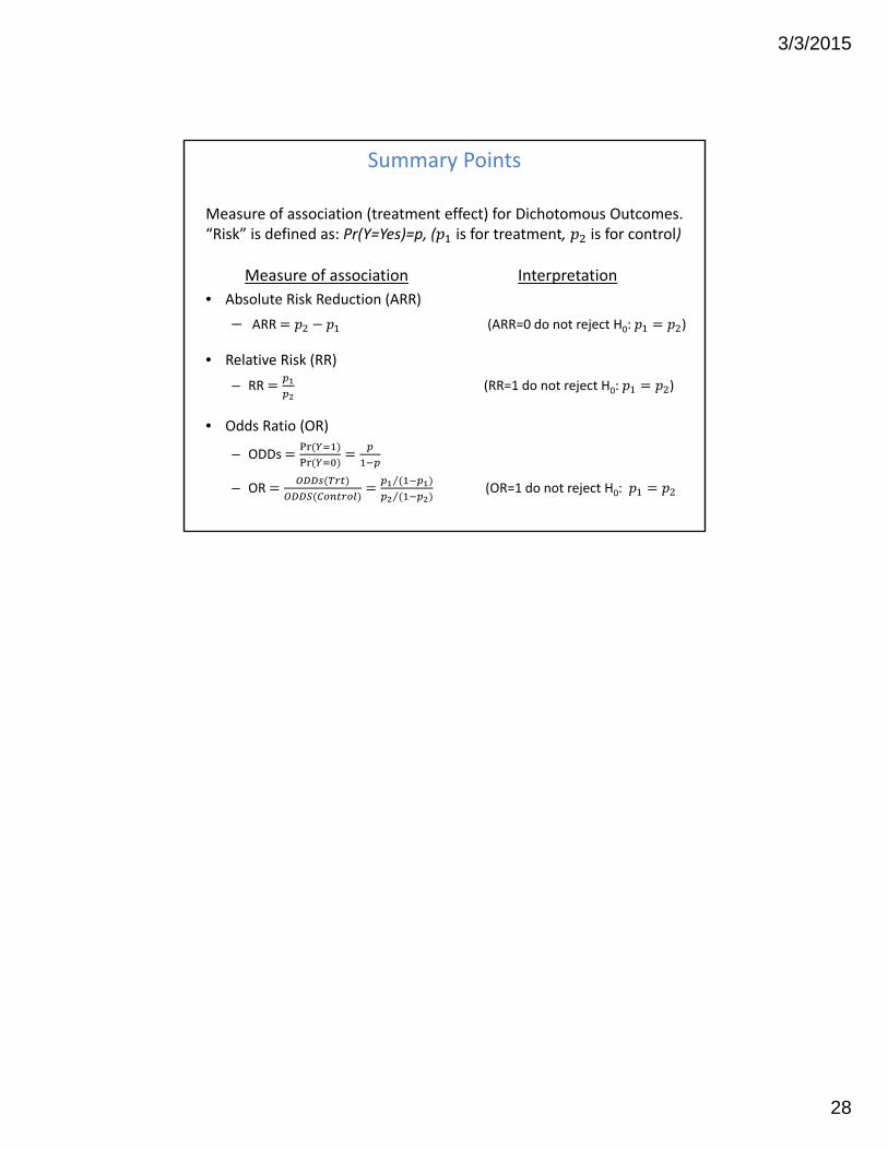
Summary Points
Measure of association (treatment effect) for Dichotomous Outcomes. “Risk” is defined as: Pr(Y=Yes)=p, ( is for treatment, is for control)
Measure of association Interpretation
• Absolute Risk Reduction (ARR)
– ARR (ARR=0 do not reject H0: )
• Relative Risk (RR)
– RR (RR=1 do not reject H0: )
• Odds Ratio (OR)
– ODDs
– OR⁄
⁄(OR=1 do not reject H0: