Binnenlandse Francqui Leerstoel VUB 2004-2005 1. Black Scholes and beyond André Farber Solvay...
33
Binnenlandse Francqui Leerstoel VUB 2004-2005 1. Black Scholes and beyond André Farber Solvay Business School University of Brussels
-
date post
21-Dec-2015 -
Category
Documents
-
view
215 -
download
2
Transcript of Binnenlandse Francqui Leerstoel VUB 2004-2005 1. Black Scholes and beyond André Farber Solvay...

Binnenlandse Francqui Leerstoel VUB 2004-20051. Black Scholes and beyond
André Farber
Solvay Business School
University of Brussels

VUB 01 Black Scholes and beyond |2August 23, 2004
Forward/Futures: Review
• Forward contract = portfolio
– asset (stock, bond, index)
– borrowing
• Value f = value of portfolio
f = S - PV(K) = S – e-rT K
Based on absence of arbitrage opportunities
• 4 inputs:
• Spot price (adjusted for “dividends” )
• Delivery price
• Maturity
• Interest rate
• Expected future price not required
VUB 01 Black Scholes and beyond |3August 23, 2004
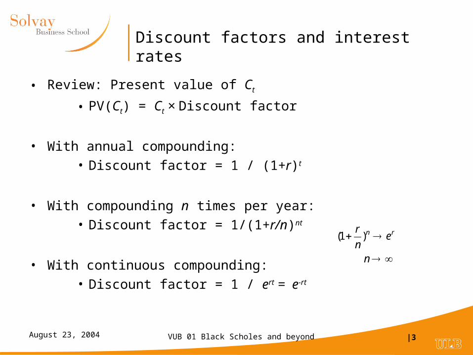
Discount factors and interest rates
• Review: Present value of Ct
• PV(Ct) = Ct × Discount factor
• With annual compounding:
• Discount factor = 1 / (1+r)t
• With compounding n times per year:
• Discount factor = 1/(1+r/n)nt
• With continuous compounding:
• Discount factor = 1 / ert = e-rt
n
en
r rn
)1(
VUB 01 Black Scholes and beyond |4August 23, 2004
Options
• Standard options
– Call, put
– European, American
• Exotic options (non standard)
– More complex payoff (ex: Asian)
– Exercise opportunities (ex: Bermudian)

VUB 01 Black Scholes and beyond |5August 23, 2004
Terminal Payoff: European call
• Exercise option if, at maturity:
Stock price > Exercice price
ST > K
• Call value at maturity
CT = ST - K if ST > K
otherwise: CT = 0
• CT = MAX(0, ST - K)
Profit at maturity
K S TStrikingprice
Stockprice
- Premium
VUB 01 Black Scholes and beyond |6August 23, 2004
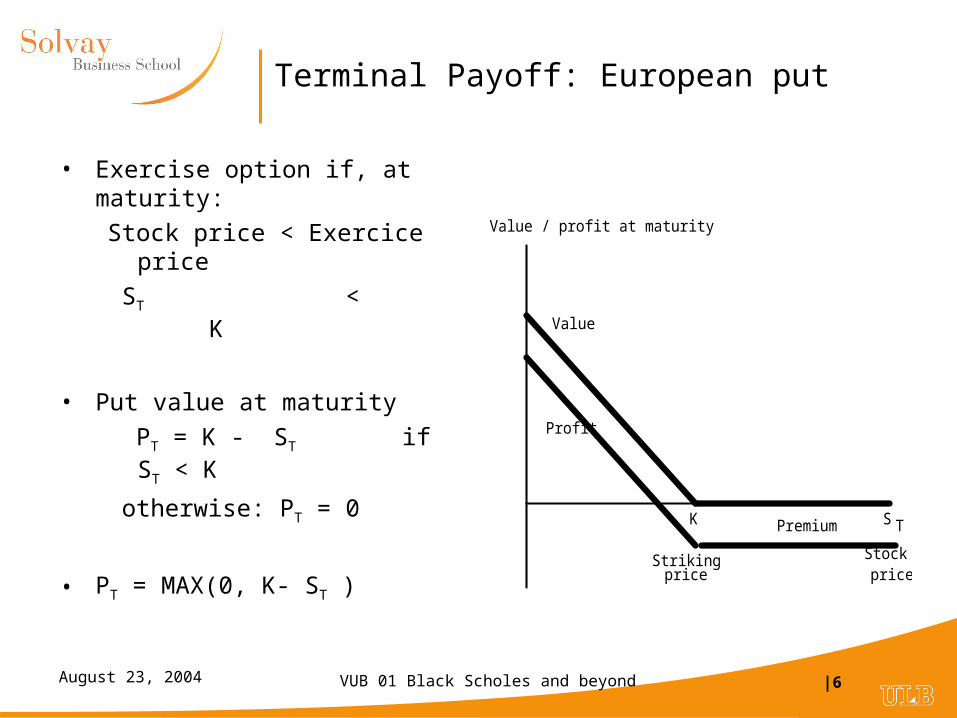
Terminal Payoff: European put
• Exercise option if, at maturity:
Stock price < Exercice price
ST < K
• Put value at maturity
PT = K - ST if ST < K
otherwise: PT = 0
• PT = MAX(0, K- ST )
Value / profit at maturity
K S T
Strikingprice
Stockprice
Value
Profit
Premium
VUB 01 Black Scholes and beyond |7August 23, 2004
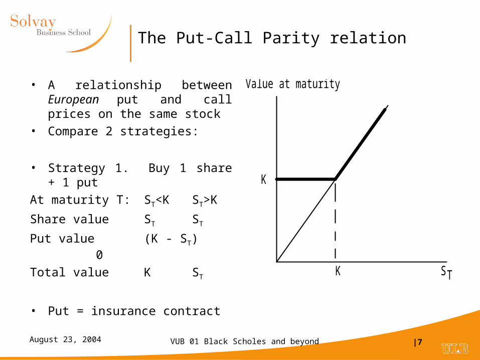
The Put-Call Parity relation
• A relationship between European put and call prices on the same stock
• Compare 2 strategies:
• Strategy 1. Buy 1 share + 1 put
At maturity T: ST<K ST>K
Share value ST ST
Put value (K - ST) 0
Total value K ST
• Put = insurance contract
K
ST
Value at maturity
K

VUB 01 Black Scholes and beyond |8August 23, 2004
Put-Call Parity (2)
• Consider an alternative strategy:
• Strategy 2: Buy call, invest PV(K)
At maturity T: ST<K ST>K
Call value 0 ST - K
Invesmt K K
Total value K ST
• At maturity, both strategies lead to the same terminal value
• Stock + Put = Call + Exercise price
K
ST
Value at maturity
K
Call
Investment
Strategy 2

VUB 01 Black Scholes and beyond |9August 23, 2004
Put-Call Parity (3)
• Two equivalent strategies should have the same cost
S + P = C + PV(K)
where S current stock price
P current put value
C current call value
PV(K) present value of the striking price
• This is the put-call parity relation
• Another presentation of the same relation:
C = S + P - PV(K)
• A call is equivalent to a purchase of stock and a put financed by borrowing the PV(K)
VUB 01 Black Scholes and beyond |10August 23, 2004
Option Valuation Models: Key ingredients
• Model of the behavior of spot price
new variable: volatility
• Technique: create a synthetic option
• No arbitrage
• Value determination
– closed form solution (Black Merton Scholes)
– numerical technique

VUB 01 Black Scholes and beyond |11August 23, 2004
Road map to valuation
Geometric Brownian Motion
dS = μSdt+σSdz
continuous timecontinuous stock prices
Binomial model uSS dS
discrete time, discrete stock prices
Model of stock price behavior
Create synthetic option
Based on Ito’s lemna to calculate df
Based on elementary algebra
Pricing equation
PDE: rffSrSff SSSt "22'' 5.0 p fu + (1-p) fd = f erΔt
Black Scholes formula
Numerical methods
VUB 01 Black Scholes and beyond |12August 23, 2004
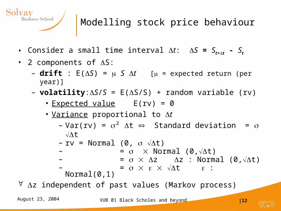
Modelling stock price behaviour
• Consider a small time interval t: S = St+t - St
• 2 components of S:– drift : E(S) = S t [ = expected return (per year)]
– volatility:S/S = E(S/S) + random variable (rv)
• Expected value E(rv) = 0
• Variance proportional to t
– Var(rv) = ² t Standard deviation = t– rv = Normal (0, t)– = Normal (0,t)– = z z :
Normal (0,t)– = t : Normal(0,1)
z independent of past values (Markov process)
VUB 01 Black Scholes and beyond |13August 23, 2004
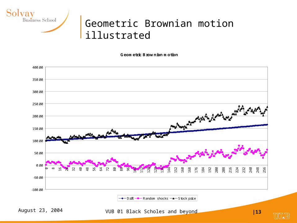
Geometric Brownian motion illustrated
Geometric Brownian motion
-100.00
-50.00
0.00
50.00
100.00
150.00
200.00
250.00
300.00
350.00
400.00
0 8 16
24
32
40
48
56
64
72
80
88
96
104
112
120
128
136
144
152
160
168
176
184
192
200
208
216
224
232
240
248
256
Drift Random shocks Stock price
VUB 01 Black Scholes and beyond |14August 23, 2004
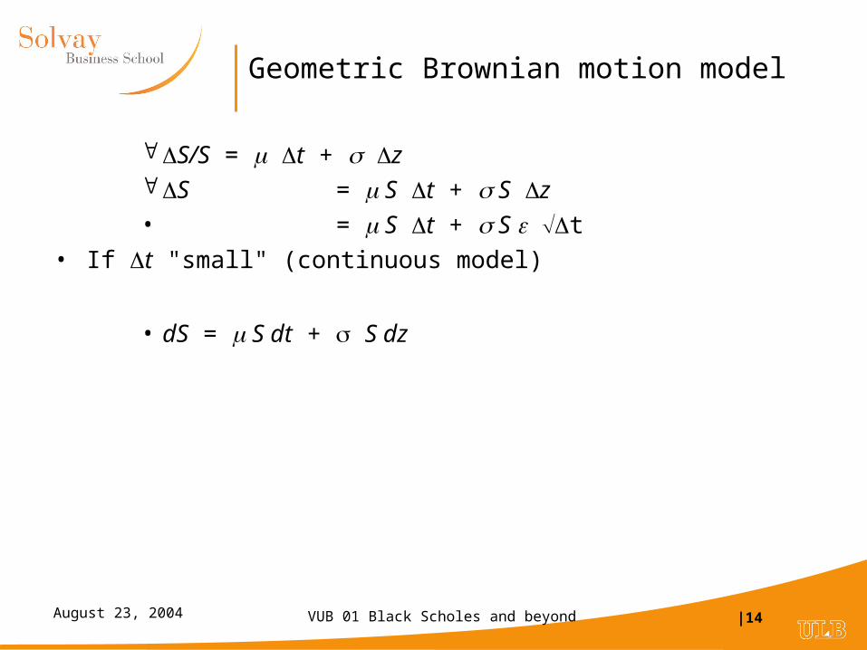
Geometric Brownian motion model
S/S = t + z S = S t + S z
• = S t + S t
• If t "small" (continuous model)
• dS = S dt + S dz
VUB 01 Black Scholes and beyond |15August 23, 2004
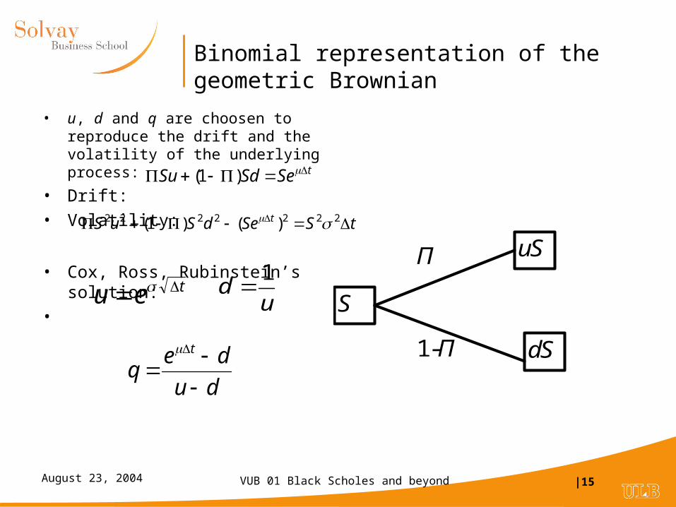
Binomial representation of the geometric Brownian
• u, d and q are choosen to reproduce the drift and the volatility of the underlying process:
• Drift:
• Volatility:
• Cox, Ross, Rubinstein’s solution:
•
S
uS
dS
Π
1-Π
teu u
d1
du
deq
t
tSeSdSu )1(
tSSedSuS t 2222222 )()1(
VUB 01 Black Scholes and beyond |16August 23, 2004
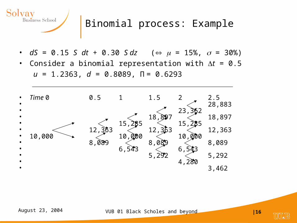
Binomial process: Example
• dS = 0.15 S dt + 0.30 S dz ( = 15%, = 30%)
• Consider a binomial representation with t = 0.5
u = 1.2363, d = 0.8089, Π = 0.6293
• Time 0 0.5 1 1.5 2 2.5• 28,883• 23,362• 18,897 18,897• 15,285 15,285• 12,363 12,363 12,363• 10,000 10,000 10,000• 8,089 8,089 8,089• 6,543 6,543• 5,292 5,292• 4,280• 3,462
VUB 01 Black Scholes and beyond |17August 23, 2004
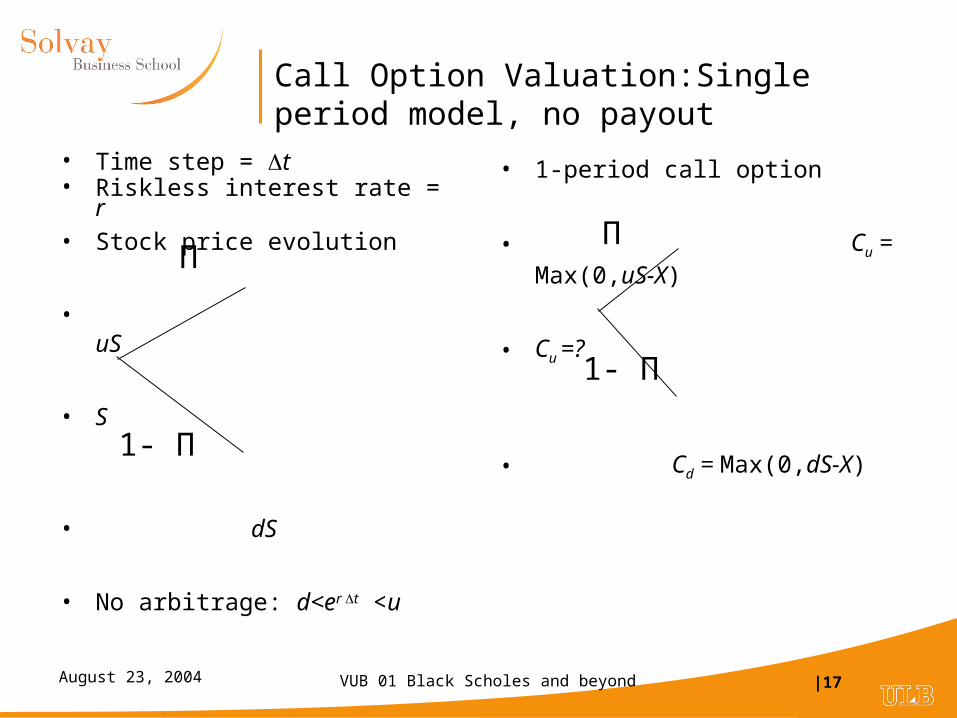
Call Option Valuation:Single period model, no payout
• Time step = t• Riskless interest rate = r • Stock price evolution
• uS
• S
• dS
• No arbitrage: d<er t <u
• 1-period call option
• Cu = Max(0,uS-X)
• Cu =?
• Cd = Max(0,dS-X)
Π
1- Π
Π
1- Π
VUB 01 Black Scholes and beyond |18August 23, 2004
Option valuation: Basic idea
• Basic idea underlying the analysis of derivative securities
• Can be decomposed into basic components possibility of creating a synthetic identical security
• by combining:
• - Underlying asset
• - Borrowing / lending
Value of derivative = value of components

VUB 01 Black Scholes and beyond |19August 23, 2004
Synthetic call option
• Buy shares
• Borrow B at the interest rate r per period
• Choose and B to reproduce payoff of call option
u S - B ert = Cu
d S - B ert = Cd
Solution:
Call value C = S - B
dSuS
CC du
trdu
edu
uCdCB
)(
VUB 01 Black Scholes and beyond |20August 23, 2004
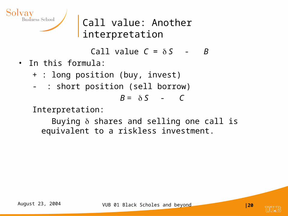
Call value: Another interpretation
Call value C = S - B
• In this formula:
+ : long position (buy, invest)
- : short position (sell borrow)
B = S - C
Interpretation:
Buying shares and selling one call is equivalent to a riskless investment.
VUB 01 Black Scholes and beyond |21August 23, 2004
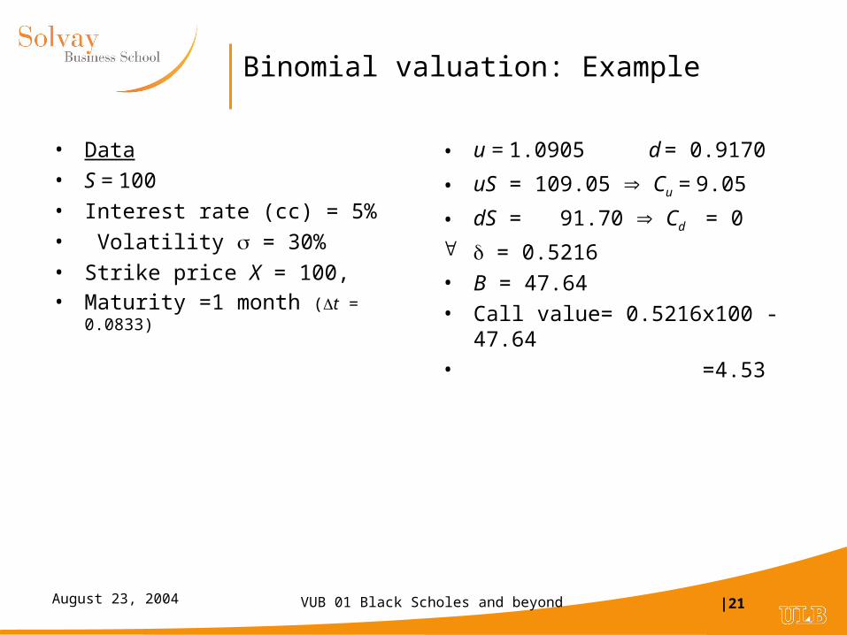
Binomial valuation: Example
• Data
• S = 100
• Interest rate (cc) = 5%
• Volatility = 30%
• Strike price X = 100, • Maturity =1 month (t = 0.0833)
• u = 1.0905 d = 0.9170
• uS = 109.05 Cu = 9.05
• dS = 91.70 Cd = 0
= 0.5216
• B = 47.64
• Call value= 0.5216x100 - 47.64
• =4.53
VUB 01 Black Scholes and beyond |22August 23, 2004
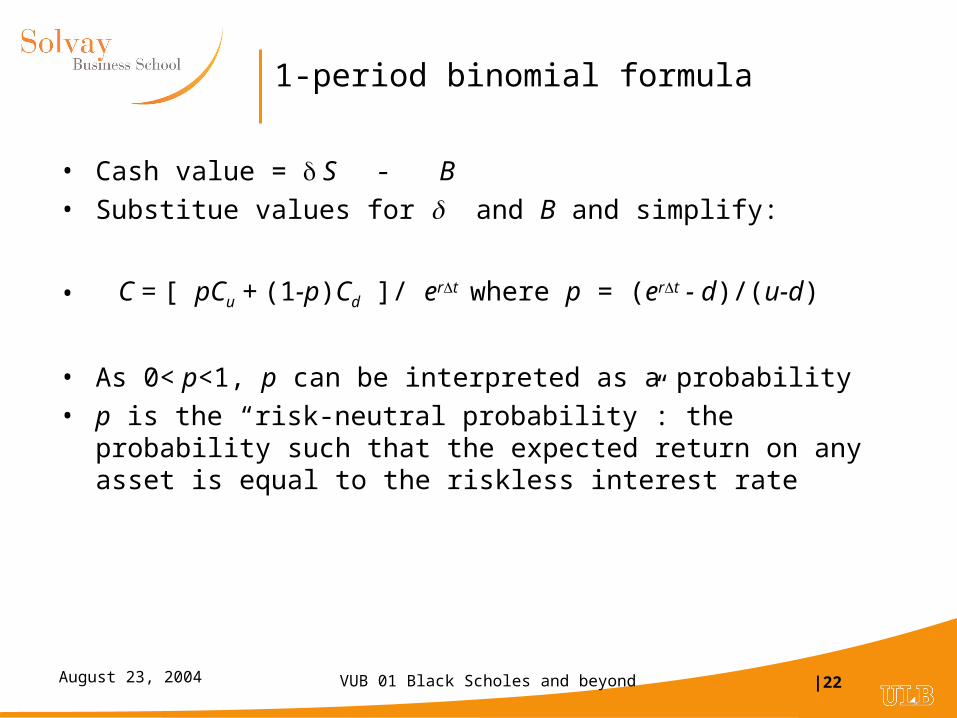
1-period binomial formula
• Cash value = S - B
• Substitue values for and B and simplify:
• C = [ pCu + (1-p)Cd ]/ ert where p = (ert - d)/(u-d)
• As 0< p<1, p can be interpreted as a probability
• p is the “risk-neutral probability”: the probability such that the expected return on any asset is equal to the riskless interest rate
VUB 01 Black Scholes and beyond |23August 23, 2004
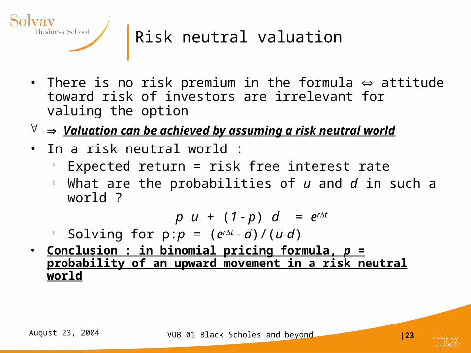
Risk neutral valuation
• There is no risk premium in the formula attitude toward risk of investors are irrelevant for valuing the option
Valuation can be achieved by assuming a risk neutral world
• In a risk neutral world : Expected return = risk free interest rate What are the probabilities of u and d in such a world ?
p u + (1 - p) d = ert
Solving for p:p = (ert - d)/(u-d)• Conclusion : in binomial pricing formula, p = probability of an upward
movement in a risk neutral world
VUB 01 Black Scholes and beyond |24August 23, 2004
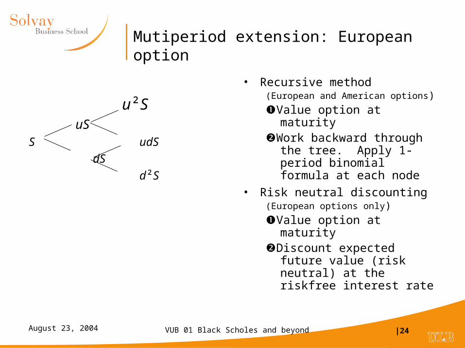
Mutiperiod extension: European option
u²SuS
S udS
dS
d²S
• Recursive method (European and American options)
Value option at maturityWork backward through the tree.
Apply 1-period binomial formula at each node
• Risk neutral discounting(European options only)
Value option at maturityDiscount expected future value
(risk neutral) at the riskfree interest rate

VUB 01 Black Scholes and beyond |25August 23, 2004
Multiperiod valuation: Example
• Data
• S = 100
• Interest rate (cc) = 5%
• Volatility = 30%
• European call option:
• Strike price X = 100,
• Maturity =2 months
• Binomial model: 2 steps
• Time step t = 0.0833
• u = 1.0905 d = 0.9170
• p = 0.5024
0 1 2 Risk neutral probability118.91 p²= 18.91 0.2524
109.05 9.46
100.00 100.00 2p(1-p)= 4.73 0.00 0.5000
91.70 0.00
84.10 (1-p)²= 0.00 0.2476
Risk neutral expected value = 4.77Call value = 4.77 e-.05(.1667) = 4.73
VUB 01 Black Scholes and beyond |26August 23, 2004
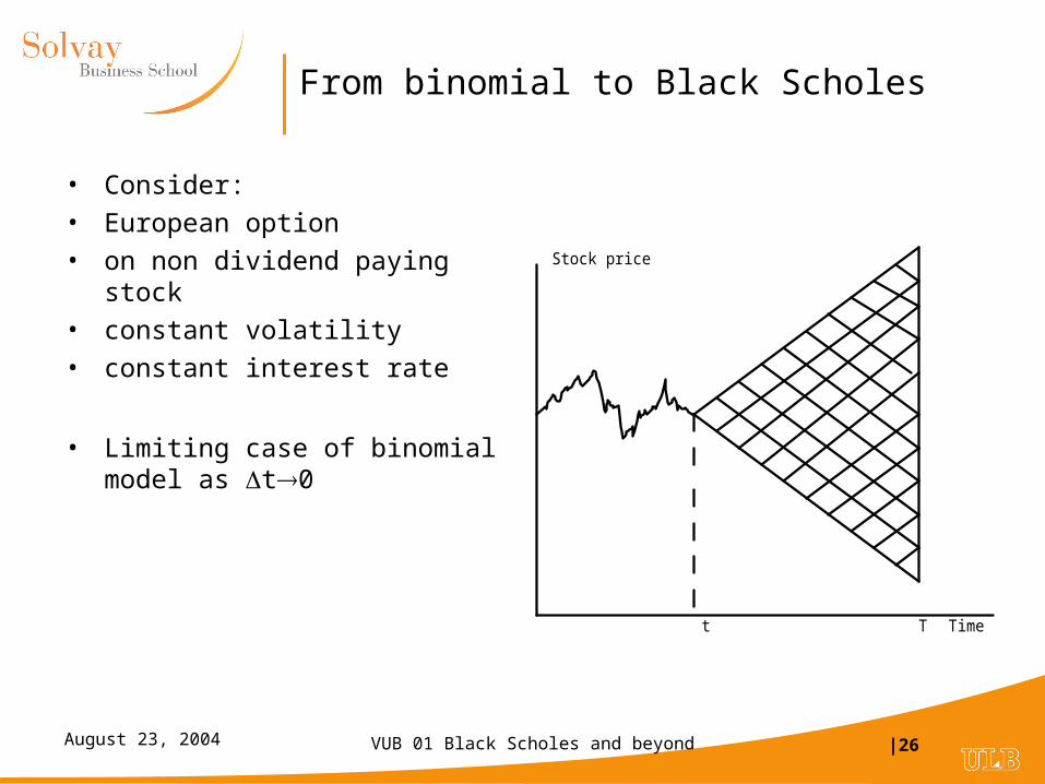
From binomial to Black Scholes
• Consider:
• European option
• on non dividend paying stock
• constant volatility
• constant interest rate
• Limiting case of binomial model as t0
Stock price
Timet T
VUB 01 Black Scholes and beyond |27August 23, 2004
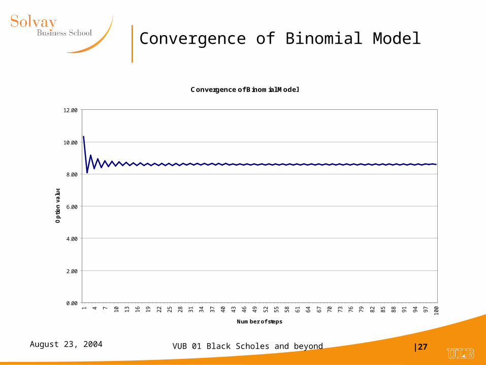
Convergence of Binomial Model
Convergence of Binomial Model
0.00
2.00
4.00
6.00
8.00
10.00
12.00
1 4 7 10
13
16
19
22
25
28
31
34
37
40
43
46
49
52
55
58
61
64
67
70
73
76
79
82
85
88
91
94
97
100
Number of steps
Op
tio
n v
alu
e

VUB 01 Black Scholes and beyond |28August 23, 2004
Arrow securities
• 2 possible states: up, down
• 2 financial assets: one riskless bond and one stock
Current price
Up Down
Bond 1 erΔt erΔt
Stock S uS dS

VUB 01 Black Scholes and beyond |29August 23, 2004
Contingent claims (digital options)
• Consider 2 securities that pay 1€ in one state and 0€ in the other state.
• They are named: contingent claims, Arrow Debreu securities, states prices
Current Price
Up Down
CC up vu 1 0
CC down vd 0 1
VUB 01 Black Scholes and beyond |30August 23, 2004
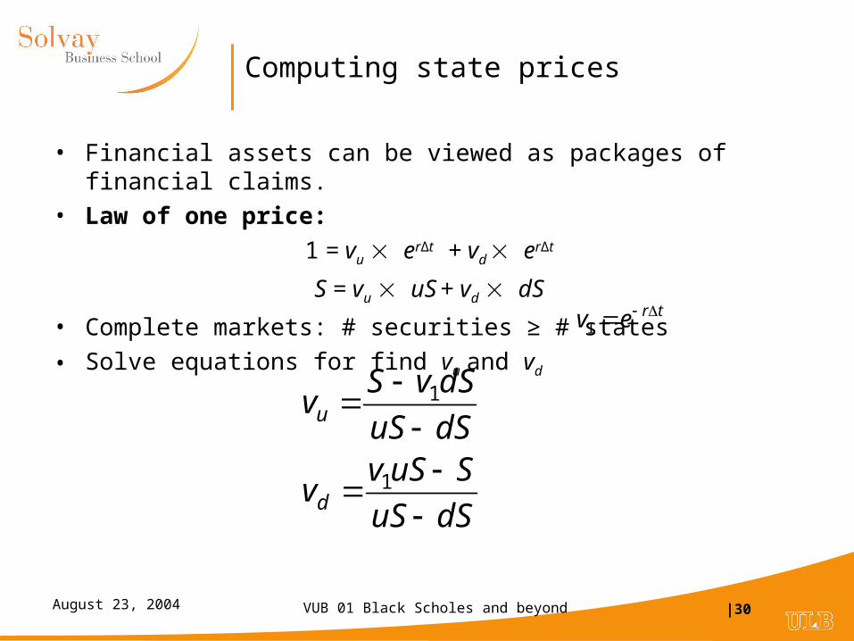
Computing state prices
• Financial assets can be viewed as packages of financial claims.
• Law of one price:
1 = vu erΔt + vd erΔt
S = vu uS + vd dS
• Complete markets: # securities ≥ # states
• Solve equations for find vu and vd
dSuS
SuSvv
dSuS
dSvSv
d
u
1
1
trev 1
VUB 01 Black Scholes and beyond |31August 23, 2004
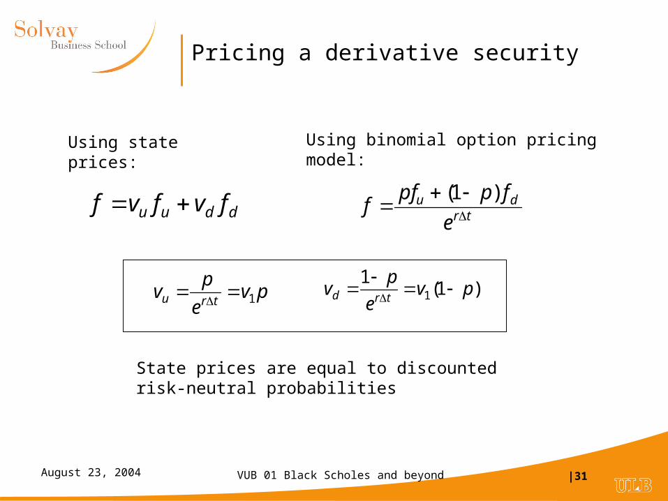
Pricing a derivative security
trdu
e
fppff
)1(dduu fvfvf
pve
pv
tru 1
Using state prices: Using binomial option pricing model:
)1(1
1 pve
pv
trd
State prices are equal to discounted risk-neutral probabilities
VUB 01 Black Scholes and beyond |32August 23, 2004
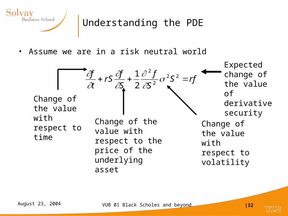
Understanding the PDE
• Assume we are in a risk neutral world
rfSS
f
S
frS
t
f 22
2
2
2
1
Expected change of the value of derivative security
Change of the value with respect to time Change of the value
with respect to the price of the underlying asset
Change of the value with respect to volatility

VUB 01 Black Scholes and beyond |33August 23, 2004
Black Scholes’ PDE and the binomial model
• We have:
• Binomial model: p fu + (1-p) fd = ert
• Use Taylor approximation:
• fu = f + (u-1) S f’S + ½ (u–1)² S² f”SS + f’t t
• fd = f + (d-1) S f’S + ½ (d–1)² S² f”SS + f’t t
• u = 1 + √t + ½ ²t
• d = 1 – √t + ½ ²t
• ert = 1 + rt
• Substituting in the binomial option pricing model leads to the differential equation derived by Black and Scholes
• BS PDE : f’t + rS f’S + ½ ² f”SS = r f