Benha University Faculty of Engineering at Shubra Dr ...

Electrical Engineering Department

Dr. Ahmed Mustafa Hussein

Benha University

Faculty of Engineering at Shubra

1 Chapter six: Modelling of Physical Systems Dr. Ahmed Mustafa Hussein

Chapter # 6 modeling of physical systems

After completing this chapter, the students will be able to:

• Find the transfer function for linear, time-invariant electrical networks,

• Obtain the transfer function for linear, time-invariant translational mechanical

systems, and draw its mechanical networks,

• Obtain the transfer function for linear, time-invariant rotational mechanical

systems (with gear train and without gear train),

• Obtain the transfer function for linear, time-invariant electromechanical

systems.

1. Introduction

This chapter presents mathematical modeling of mechanical systems, electrical

systems and electromechanical systems.

Mechanical systems can be either translational or rotational. Although the

fundamental relationships for both types are derived from Newton’s law, they are

different enough to warrant separate considerations.



Benha University



Any physical system consists of mechanical elements. There are three types of basic

elements in such kind of systems:

Translational Motion Rotational Motion

Mass elements Moment of Inertia elements

Linear Spring elements Torsional Spring elements

Linear Dampers elements Torsional Damper elements

Example of physical system that has rotary motion is the Antenna Azimuth Position

Control System shown in Figure below.

(a) Layout of the system

(b) schematic diagram of the system



Benha University



(c) Block diagram of the system

2. Mass / Inertia element

Newton’s law (translational motion): If a force (F) is acting on rigid body through the

center of mass (M) in a given direction, the acceleration (a) of the rigid body in the

same direction is directly proportional to the force acting on it and is inversely

proportional to the mass of the body. That is,

𝑎𝑐𝑐𝑒𝑙𝑒𝑟𝑎𝑡𝑖𝑜𝑛 (𝑎) =𝐹𝑜𝑟𝑐𝑒 (𝐹)

𝑀𝑎𝑠𝑠 (𝑀) 𝑂𝑅 𝐹 = 𝑀 × 𝑎 = 𝑀

𝑑𝑣

𝑑𝑡= 𝑀

𝑑2𝑥

𝑑𝑡2

Suppose that there are many forces acting on a body of mass, then

∑𝐹 = 𝑀 × 𝑎

Newton’s law (Rotational motion):

𝑎𝑛𝑔𝑢𝑙𝑎𝑟 𝑎𝑐𝑐𝑒𝑙𝑒𝑟𝑎𝑡𝑖𝑜𝑛 (𝛼) =𝑇𝑜𝑟𝑞𝑢𝑒 (𝑇)

𝐼𝑛𝑒𝑟𝑡𝑖𝑎 (𝐽) 𝑂𝑅 𝑇 = 𝐽 × 𝛼 = 𝐽

𝑑𝜔

𝑑𝑡= 𝐽

𝑑2𝜃

𝑑𝑡2

Suppose that there are many torques acting on a rotating body of inertia, then

∑𝑇 = 𝐽 × 𝛼



Benha University



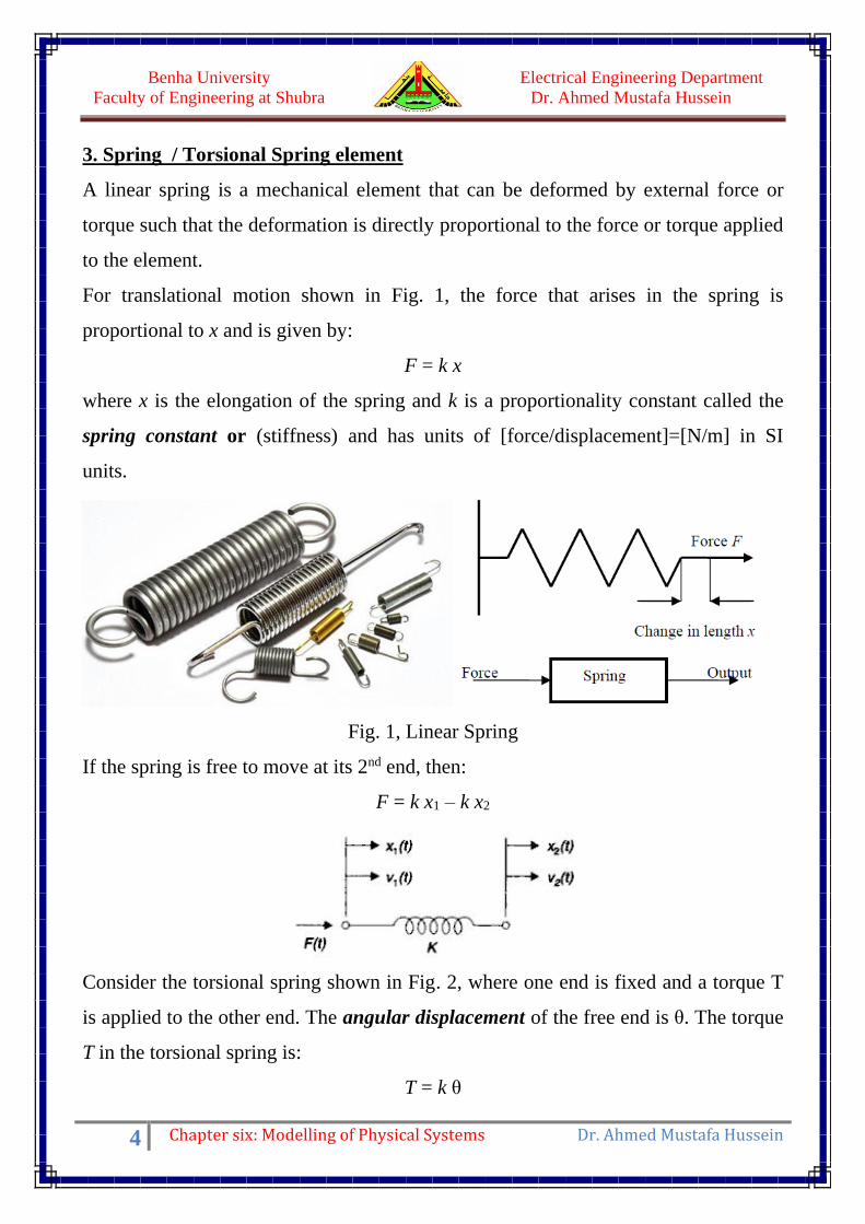
3. Spring / Torsional Spring element

A linear spring is a mechanical element that can be deformed by external force or

torque such that the deformation is directly proportional to the force or torque applied

to the element.

For translational motion shown in Fig. 1, the force that arises in the spring is

proportional to x and is given by:

F = k x

where x is the elongation of the spring and k is a proportionality constant called the

spring constant or (stiffness) and has units of [force/displacement]=[N/m] in SI

units.

Fig. 1, Linear Spring

If the spring is free to move at its 2nd end, then:

F = k x1 – k x2

Consider the torsional spring shown in Fig. 2, where one end is fixed and a torque T

is applied to the other end. The angular displacement of the free end is θ. The torque

T in the torsional spring is:

T = k θ



Benha University



where θ is the angular displacement and k is the spring constant or (stiffness) for

torsional spring and has units of [Torque/angular displacement]=[N-m/rad] in SI

units.

Fig. 2, Torsional Spring

If the spring is free to move at its 2nd end, then:

T = k 1 – k 2

4. Damper (Dashpot)

A damper is a mechanical element that dissipates energy in the form of heat instead

of storing it. Figure 4 shows a schematic diagram of a translational damper, or a

dashpot that consists of a piston and an oil-filled cylinder. Any relative motion

between the piston rod and the cylinder is resisted by oil.

Fig. 4, Translational Damper

In the damper, the damping force F that arises in it is proportional to the velocity,

𝐹 = 𝐵 �̇�



Benha University



Where B relating the damping force F to the velocity and called the viscous friction

coefficient. The dimension of b is [force/Velocity] = [N.s/m] in SI units.

For the torsional damper shown in Fig. 5, the torque T applied to the ends of the

damper is:

𝑇 = 𝐵 �̇�

Where B relating the damping torque T to the angular velocity and called the viscous

friction coefficient. The dimension of B is [torque/angular velocity] = [N.m.s/rad] in

SI units.



Benha University



Example (1):

Write the differential equations describing systems shown in Fig. 6.

Fig. 6: a) parallel springs b) series springs

For system in Fig. 6. a)

𝐹 = 𝑘1𝑥 + 𝑘2𝑥

For system in Fig. 6. b)

𝐹 = 𝑘2(𝑥 − 𝑦) (𝑎𝑡 𝑛𝑜𝑑𝑒 𝑥)

0 = 𝑘1𝑦 + 𝑘2(𝑦 − 𝑥) (𝑎𝑡 𝑛𝑜𝑑𝑒 𝑦)

Example (2):

For the mechanical system shown in Fig. 7, draw the mechanical network and write

the D.E at each node.

Fig. 7, One-mass mechanical system

The mechanical network is:



Benha University



At node x1 :

f(t) = k (x1 – x2)

F(s) = k X1(s) – k X2(s)

At node x2 :

2212 )(0 xBxMxxk ++−=

0 = k X2(s) – k X1(s) – M S2X2(s) + B SX2(s)

Example (3):

Obtain the transfer functions X1(s)/F(s) of the mechanical system shown in Fig. 8.

Fig. 8, Two-mass mechanical system

Mechanical network

Writing the D.E. at the displacement x1:

𝑓(𝑡) = 𝑚1�̈�1 + 𝑏(�̇�1 − �̇�2) + 𝑘1𝑥1 + 𝑘2(𝑥1 − 𝑥2)

Taking Laplace:

𝐹(𝑠) = 𝑚1𝑆2𝑋1(𝑠) + 𝑏𝑆𝑋1(𝑠) − 𝑏𝑆𝑋2(𝑠) + 𝑘1𝑋1(𝑠) + 𝑘2𝑋1(𝑠) − 𝑘2𝑋2(𝑠)

𝐹(𝑠) = 𝑋1(𝑠)[𝑚1𝑆2 + 𝑏𝑆 + 𝑘1 + 𝑘2] − 𝑋2(𝑠)[𝑏𝑆 + 𝑘2] (1)



Benha University




0 = 𝑚2�̈�2 + 𝑏(�̇�2 − �̇�1) + 𝑘2(𝑥2 − 𝑥1) + 𝑘3𝑥2

Taking Laplace:

0 = 𝑚2𝑆2𝑋2(𝑠) + 𝑏𝑆𝑋2(𝑠) − 𝑏𝑆𝑋1(𝑠) + 𝑘2𝑋2(𝑠) + 𝑘3𝑋2(𝑠) − 𝑘2𝑋1(𝑠)

0 = 𝑋2(𝑠)[𝑚2𝑆2 + 𝑏𝑆 + 𝑘2 + 𝑘3] − 𝑋1(𝑠)[𝑏𝑆 + 𝑘2] (2)

From Eqn. (2):

𝑋2(𝑠) =𝑏𝑆 + 𝑘2

𝑚2𝑆2 + 𝑏𝑆 + 𝑘2 + 𝑘3

𝑋1(𝑠)

Substituting with the value of X2(s) in eqn. (1)

𝐹(𝑠) = 𝑋1(𝑠)[𝑚1𝑆2 + 𝑏𝑆 + 𝑘1 + 𝑘2] −

(𝑏𝑆 + 𝑘2)2

𝑚2𝑆2 + 𝑏𝑆 + 𝑘2 + 𝑘3

𝑋1(𝑠)

𝐹(𝑠) =(𝑚1𝑆

2 + 𝑏𝑆 + 𝑘1 + 𝑘2)(𝑚2𝑆2 + 𝑏𝑆 + 𝑘2 + 𝑘3) − (𝑏𝑆 + 𝑘2)

2

𝑚2𝑆2 + 𝑏𝑆 + 𝑘2 + 𝑘3

𝑋1(𝑠)

Then

𝑋1(𝑠)

𝐹(𝑠)=

𝑚2𝑆2 + 𝑏𝑆 + 𝑘2 + 𝑘3

(𝑚1𝑆2 + 𝑏𝑆 + 𝑘1 + 𝑘2)(𝑚2𝑆

2 + 𝑏𝑆 + 𝑘2 + 𝑘3) − (𝑏𝑆 + 𝑘2)2

Example (4):

For a car suspension shown in Fig. 8,



Benha University



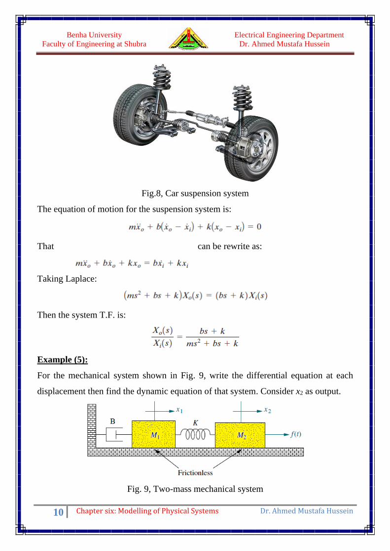
Fig.8, Car suspension system

The equation of motion for the suspension system is:

That can be rewrite as:

Taking Laplace:

Then the system T.F. is:

Example (5):

For the mechanical system shown in Fig. 9, write the differential equation at each

displacement then find the dynamic equation of that system. Consider x2 as output.

Fig. 9, Two-mass mechanical system



Benha University



Let v1, x1, v2 and x2 are the state variables

We know that:

𝑑𝑥1

𝑑𝑡= 𝑣1 𝑎𝑛𝑑

𝑑𝑥2

𝑑𝑡= 𝑣2


𝑓(𝑡) = 𝑀2�̈�2 + 𝑘(𝑥2 − 𝑥1)

𝑓(𝑡) = 𝑀2�̇�2 + 𝑘(𝑥2 − 𝑥1)

�̇�2 =1

𝑀2𝑓(𝑡) −

𝑘

𝑀2𝑥2 +

𝑘

𝑀2𝑥1


0 = 𝑀1�̈�1 + 𝐵�̇�1 + 𝑘(𝑥1 − 𝑥2)

�̇�1 = −𝐵

𝑀1𝑣1 −

𝑘

𝑀1𝑥1 +

𝑘

𝑀1𝑥2

[

�̇�1

�̇�1

�̇�2

�̇�2

] =

[

0 1 0 0

−𝑘

𝑀1−

𝐵

𝑀1

𝑘

𝑀1 0

0𝑘

𝑀2

00

0 1

−𝑘

𝑀20]

[

𝑥1

𝑣1𝑥2

𝑣2

] +

[ 0001

𝑀2]

𝑢(𝑡)

[𝑦] = [0 0 1 0] [

𝑥1

𝑣1𝑥2

𝑣2

]

Example (6):

Find the T.F. 2(s)/T(s) for the rotational mechanical system shown in Fig. 10.

Fig. 10, Rotational mechanical system

Writing the D.E. at the angular displacement 1:



Benha University



𝑇(𝑡) = 𝐽1�̈�1 + 𝐵1�̇�1 + 𝑘(𝜃1 − 𝜃2)

Taking Laplace:

𝑇(𝑠) = 𝐽1𝑆2𝜃1(𝑠) + 𝐵1𝑆𝜃1(𝑠) + 𝑘𝜃1(𝑠) − 𝑘𝜃2(𝑠)

𝑇(𝑠) = 𝜃1(𝑠)[𝐽1𝑆2 + 𝐵1𝑆 + 𝑘] − 𝑘 𝜃2(𝑠) (1)

Writing the D.E. at the angular displacement 2:

0 = 𝐽2�̈�2 + 𝐵2�̇�2 + 𝑘(𝜃2 − 𝜃1)

Taking Laplace:

0 = 𝐽2𝑆2𝜃2(𝑠) + 𝐵2𝑆𝜃2(𝑠) + 𝑘𝜃2(𝑠) − 𝑘𝜃1(𝑠)

0 = 𝜃2(𝑠)[𝐽2𝑆2 + 𝐵2𝑆 + 𝑘] − 𝑘 𝜃1(𝑠) (2)

From Eqn. (2):

𝜃1(𝑠) =[𝐽2𝑆

2 + 𝐵2𝑆 + 𝑘]

𝑘𝜃2(𝑠)

Substituting with the value of 2(s) in eqn. (1),

𝑇(𝑠) =[𝐽2𝑆

2 + 𝐵2𝑆 + 𝑘]

𝑘[𝐽1𝑆

2 + 𝐵1𝑆 + 𝑘]𝜃2(𝑠) − 𝑘 𝜃2(𝑠)

𝑇(𝑠) =[𝐽2𝑆

2 + 𝐵2𝑆 + 𝑘][𝐽1𝑆2 + 𝐵1𝑆 + 𝑘] − 𝑘2

𝑘𝜃2(𝑠)

Then the system T.F. is:

𝜃2(𝑠)

𝑇(𝑠)=

𝑘

[𝐽2𝑆2 + 𝐵2𝑆 + 𝑘][𝐽1𝑆

2 + 𝐵1𝑆 + 𝑘] − 𝑘2

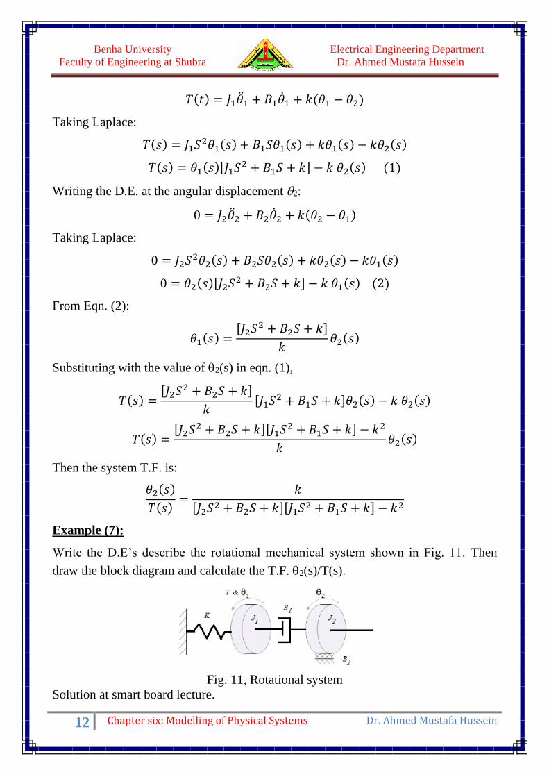
Example (7):

Write the D.E’s describe the rotational mechanical system shown in Fig. 11. Then

draw the block diagram and calculate the T.F. 2(s)/T(s).

Fig. 11, Rotational system

Solution at smart board lecture.



Benha University



Example (8):

For the linear displacement mechanical system shown below, draw the mechanical

network, then write the D.E’s that describe the system and draw the block diagram

where x1(t) is the desired output

The mechanical network for this system is:



Benha University



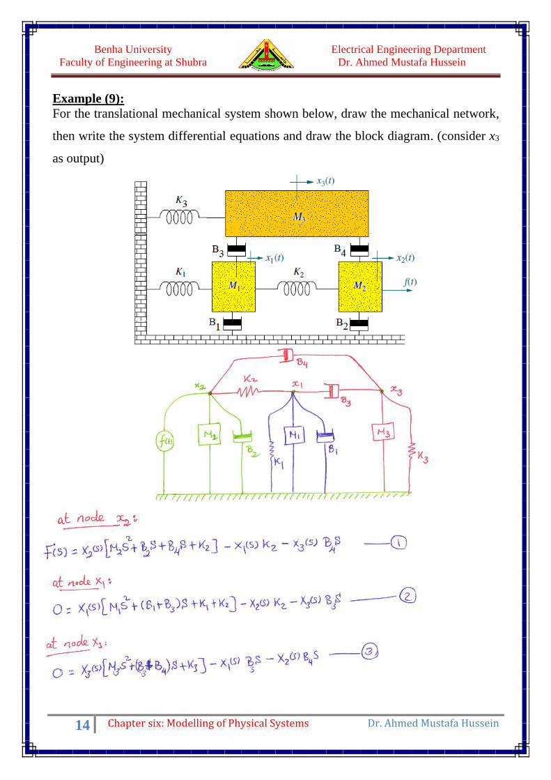
Example (9):

For the translational mechanical system shown below, draw the mechanical network,

then write the system differential equations and draw the block diagram. (consider x3

as output)



Benha University



5. Mechanical Systems with Gears

Gear is a toothed machine part, such as a wheel or cylinder that meshes with another

toothed part to transmit motion or to change speed or direction.

In industrial applications, generally gears associate to a motor which drives the load.

Gears are used to obtain more speed and less torque or less speed and more torque.

The interaction between two gears is depicted in the Fig. 12. An input gear with

radius r1 and N1 teeth is rotated through angle 1(t) due to a torque, T1(t). An output

gear with radius r2 and N2 teeth responds by rotating through angle 2(t) and

delivering a torque, T2(t).

Fig. 12, Two-Gear transmission system

Also we must note that, if the number of gear is even, the direction of motion is

reversed. But if it is odd, as shown in Fig. 13, the direction of motion is not reversed.



Benha University



Fig. 13, Three-Gear transmission system

What is the relationship between the input torque, T1 and the delivered torque, T2 ?

Assuming the gears do not absorb or store energy (ideal gear), then the input energy

of Gear 1 equals the energy out of Gear 2.

𝑇1 × 𝜃1 = 𝑇2 × 𝜃2

Therefore,

𝑇1

𝑇2=

𝜃2

𝜃1=

𝑁1

𝑁2

These relations can be summarized in blocks as:

Example (10):

For the gear train shown in Fig. 14, a load is driven by a motor through the gear train.

Assuming the stiffness of the motor shaft is infinite, draw the block diagram and find

the T.F. 2(s)/Tm(s).

Fig. 14, Gear train system



Benha University



At node 1:

𝑇𝑚(𝑡) = (𝐽𝑚 + 𝐽1)�̈�1 + 𝐵𝑚�̇�1 + 𝑇1(𝑡)

𝑇𝑚(𝑠) = 𝜃1(𝑠)[ (𝐽𝑚 + 𝐽1)𝑆2 + 𝐵𝑚𝑆 ] + 𝑇1(𝑠) (1)

At node 2:

𝑇2(𝑡) = (𝐽2 + 𝐽𝐿)�̈�2 + 𝐵(�̇�2) + 𝑘 𝜃2

𝑇2(𝑠) = 𝜃2(𝑠)[ (𝐽2+𝐽𝐿)𝑆2 + 𝐵𝑆 + 𝑘] (2)

Also we must consider the two relations of the gear train:

𝑇1

𝑇2=

𝜃2

𝜃1=

𝑁1

𝑁2

From the above eqns., we can draw the block diagram:

So you can easily calculate the system T.F. 2(s)/Tm(s)

Example (11):

For the rotational mechanical system given below,

a) Write the differential equations that represent that system,

b) Draw the block diagram considering T(s) as input and L(s) as an output.

The D.E’s that describe the mechanical system are:

T(s) = 1(s)[50 S2 + 0.1] + T1(s)

1

(𝐽𝑚 + 𝐽1)𝑆2 + 𝐵𝑚𝑆

Tm(S) + 2 (S)

_

𝑁1

𝑁2

𝑁1

𝑁2 (𝐽𝑚 + 𝐽1)𝑆

2 + 𝐵𝑚𝑆 + 𝑘 T2(S)

1(S)

T1(S)



Benha University



T2(s) = 2(s)[100 S2 +100 S + 100] + T3(s)

T4(s) = L(s)[200 S + 2] - 3(s)[2]

0 = 3(s)[3 S + 2] - L(s)[2]

𝑁1

𝑁2=

30

100=

𝑇1

𝑇2=

𝜃2

𝜃1

𝑁3

𝑁4=

10

100=

𝑇3

𝑇4=

𝜃𝐿

𝜃2

The above equations can be represented in block diagram as:

Example (12):

For the rotational mechanical system given below,

a) Write the differential equations that represent that system,

b) Draw the block diagram considering T(s) as input and L(s) as an output.

The D.E’s that describe the mechanical system are:

T(s) = 1(s)[50 S2 + 200S + 0.1] + T1(s)

T2(s) = 2(s)[2] - 3(s)[2]



Benha University



0 = 3(s)[ 10 S2 + 3S + 2] - 2(s)[2] + T3(s)

T4(s) = L(s)[ 100 S2 + 200S]

𝑁1

𝑁2=

30

300=

𝑇1

𝑇2=

𝜃2

𝜃1

𝑁3

𝑁4=

10

100=

𝑇3

𝑇4=

𝜃𝐿

𝜃3

The above equations can be represented in block diagram as:

6. Modeling of Electrical Systems

A mathematical model of an electrical circuit can be obtained by applying one or both

of Kirchhoff’s laws to it.

RC Circuit: Consider the electrical circuit shown in Fig. 15. The circuit consists of a

resistance R (ohm), and a capacitance C (farad).

Fig. 15. RC circuit

The equations of this RC circuit are:



Benha University



Combining the above two blocks we get the overall block diagram of the RC circuit;

𝐸𝑜(𝑠)

𝐸𝑖(𝑠)=

1

1 + 𝑅𝐶𝑠

RLC Circuit: Consider the electrical circuit shown in Fig. 16. The circuit consists of

an inductance L (henry), a resistance R (ohm), and a capacitance C (farad).

Fig. 16, RLC circuit

Applying Kirchhoff’s voltage law to the system, we obtain the following equations:

Taking Laplace:

𝐸𝑖(𝑠) = 𝐼(𝑠) {𝐿𝑠 + 𝑅 +1

𝐶𝑠} =

𝐿𝐶𝑠2 + 𝑅𝐶𝑠 + 1

𝐶𝑠𝐼(𝑠)

𝐸𝑜(𝑠) = 𝐼(𝑠){1

𝐶𝑠}

The block diagram is given below:

From which the T.F. is:

A state-space model of that system may be obtained as follows:

First, note that the differential equation for the system can be obtained from T.F. as

Assuming the state variables as:



Benha University



Repeated RC circuit: as shown in Fig. 17, we need to obtain the T.F. of this circuit.

Therefore the D.E’s. that describe the circuit are as follows:

Fig. 17. Cascaded RC circuit

Example (13):

Obtain the transfer function Xo(s)/Xi(s) of the mechanical system shown in Fig. 18

(a). Also obtain the transfer function Eo(s)/Ei(s) of the electrical system shown in Fig.

18 (b). Show that these transfer functions of the two systems are of identical form and

thus they are analogous systems.



Benha University



Fig. 18, (a) Mechanical system (b) analogous electrical system

From mechanical system:

Taking Laplace:

From the electrical system:

7. Modeling of DC Machines:

Direct-current (DC) motors are one of the most widely used prime movers in the

industry. Years ago, the majority of the small servomotors used for control purposes

were ac. In reality, ac motors are more difficult to control, especially for position



Benha University



control, and their characteristics are quite nonlinear, which makes the analytical task

more difficult. DC motors, on the other hand, are more expensive, because of their

brushes and commutators, and variable-flux DC motors are suitable only for certain

types of control applications. Before permanent-magnet technology was fully

developed, the torque-per-unit volume or weight of a DC motor with a permanent-

magnet (PM) field was far from desirable. Today, with the development of the rare-

earth magnet, it is possible to achieve very high torque-to-volume PM DC motors at

reasonable cost. Furthermore, the advances made in brush-and-commutator

technology have made these wearable parts practically maintenance-free. The

advancements made in power electronics have made brushless dc motors quite

popular in high-performance control systems. Advanced manufacturing techniques

have also produced dc motors with ironless rotors that have very low inertia, thus

achieving a very high torque-to-inertia ratio. Low-time-constant properties have

opened new applications for dc motors in computer peripheral equipment such as

tape drives, printers, disk drives, and word processors, as well as in the automation

and machine-tool industries.

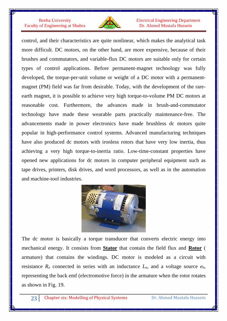
The dc motor is basically a torque transducer that converts electric energy into

mechanical energy. It consists from Stator that contain the field flux and Rotor (

armature) that contains the windings. DC motor is modeled as a circuit with

resistance Ra connected in series with an inductance La, and a voltage source eb,

representing the back emf (electromotive force) in the armature when the rotor rotates

as shown in Fig. 19.



Benha University



The torque developed (Tm) on the motor shaft is directly proportional to the field flux

() and the armature current (Ia).

𝑇𝑚(𝑡) = 𝑘∅ 𝑖𝑎(𝑡)

If the flux is kept constant

𝑇𝑚(𝑡) = 𝑘𝑖𝑖𝑎(𝑡)

Also the induced emf eb is directly proportional to the field flux () and the shaft

speed (m).

𝑒𝑏(𝑡) = 𝑘∅ 𝜔𝑚(𝑡)

If the flux is kept constant

𝑒𝑏(𝑡) = 𝑘𝑏 𝜔𝑚(𝑡)

Fig. 19, Separately-Excited DC motor circuit

Electrical Equation:

𝑒𝑎(𝑡) = 𝑅𝑎𝑖𝑎(𝑡) + 𝐿𝑎

𝑑𝑖𝑎𝑑𝑡

+ 𝑒𝑏(𝑡)

𝑑𝑖𝑎𝑑𝑡

=1

𝐿𝑎𝑒𝑎(𝑡) −

𝑅𝑎

𝐿𝑎𝑖𝑎(𝑡) −

1

𝐿𝑎𝑒𝑏(𝑡)



Benha University



Mechanical Equation:

𝑇𝑚(𝑡) = 𝐽𝑚�̈�𝑚(𝑡) + 𝐵𝑚�̇�𝑚(𝑡) + 𝑇𝐿

�̈�𝑚(𝑡) =1

𝐽𝑚𝑇𝑚(𝑡) −

𝐵𝑚

𝐽𝑚�̇�𝑚(𝑡) −

1

𝐽𝑚𝑇𝐿

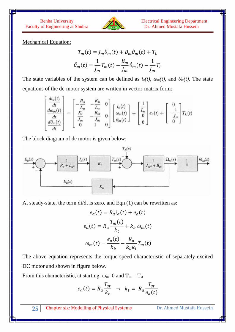
The state variables of the system can be defined as ia(t), m(t), and m(t). The state

equations of the dc-motor system are written in vector-matrix form:

The block diagram of dc motor is given below:

At steady-state, the term di/dt is zero, and Eqn (1) can be rewritten as:

𝑒𝑎(𝑡) = 𝑅𝑎𝑖𝑎(𝑡) + 𝑒𝑏(𝑡)

𝑒𝑎(𝑡) = 𝑅𝑎

𝑇𝑚(𝑡)

𝑘𝑡+ 𝑘𝑏 𝜔𝑚(𝑡)

𝜔𝑚(𝑡) =𝑒𝑎(𝑡)

𝑘𝑏−

𝑅𝑎

𝑘𝑏𝑘𝑡𝑇𝑚(𝑡)

The above equation represents the torque-speed characteristic of separately-excited

DC motor and shown in figure below.

From this characteristic, at starting: ωm=0 and Tm = Tst

𝑒𝑎(𝑡) = 𝑅𝑎

𝑇𝑠𝑡

𝑘𝑡 → 𝑘𝑡 = 𝑅𝑎

𝑇𝑠𝑡

𝑒𝑎(𝑡)



Benha University



At no load, the speed is no-load speed (ωnL) and the torque is zero, Tm = 0

𝜔𝑛𝐿(𝑡) =𝑒𝑎(𝑡)

𝑘𝑏 → 𝑘𝑏 =

𝑒𝑎(𝑡)

𝜔𝑛𝐿

From the above two equations, the electrical constants kt & kb can be determined.

Example (13)

For the separately-excited DC motor with torque-speed characteristic given below,

draw the block diagram then find the transfer function L(S)/Ea(S). Take the armature

resistance and inductance are 0.06 and 0.2 H respectively.

From the torque-Speed characteristic above, ωnL=50 rad/s, Tst=500 N.m at Ea 100V.

Therefore, the motor constants can be obtained as:

𝑘𝑡 = 𝑅𝑎

𝑇𝑠𝑡

𝑒𝑎(𝑡)=

0.06 × 500

100= 0.3 𝑁.𝑚/𝐴

𝑘𝑏 =𝑒𝑎(𝑡)

𝜔𝑛𝐿=

100

50= 2 𝑉. 𝑠/𝑟𝑎𝑑

Electrical equation at constant flux (S-domain):



Benha University



𝐸𝑎(𝑆) = 𝐼𝑎(𝑆)[𝑅𝑎 + 𝐿𝑎𝑆] + 𝑘𝑏𝜔(𝑆)

𝐸𝑎(𝑆) = 𝐼𝑎(𝑆)[0.06 + 0.2 𝑆] + 2𝑆 𝜃(𝑆)

The electromagnetic torque Tm(S) = kt Ia(S) = 0.3 Ia(S)

Mechanical equation at constant flux (S-domain):

𝑇𝑚(𝑆) = 𝜃𝑚(𝑆)[𝐽1𝑆2 + 𝐵1𝑆] + 𝑇1

𝑇𝑚(𝑆) = 𝜃𝑚(𝑆)[5𝑆2 + 2𝑆] + 𝑇1

From the gear ratio:

𝜃𝐿(𝑆)

𝜃𝑚(𝑆)=

𝑁1

𝑁2=

100

1000=

1

10

At load:

𝑇2(𝑆) = 𝜃𝐿(𝑆)[𝐽2𝑆2 + 𝐵2𝑆]

𝑇2(𝑆) = 𝜃𝐿(𝑆)[700 𝑆2 + 800 𝑆]

From the gear ratio:

𝑇1(𝑆)

𝑇2(𝑆)=

𝑁1

𝑁2=

100

1000=

1

10

The block diagram is given in figure below.

Example (15):

Consider the speed control system shown in Fig. 20. The armature of the motor is

supplied with a controlled voltage through a DC generator. The generator field

current controls the generated voltage Eg. Draw the block diagram representing this

system and deduce the T.F. m(s)/Ei(s)



Benha University



Fig. 20, Motor-Generator system

The D.E’s that describe the motor-generator set are:

𝐸𝑖(𝑠) − 𝑘𝑏𝜔𝑚(𝑠) = 𝑒(𝑠)

𝐴 𝑒(𝑠) = 𝐼𝑓(𝑠)[𝑅𝑓 + 𝑆𝐿𝑓]

𝐸𝑔(𝑠) = 𝑘𝑔𝐼𝑓(𝑠)

𝐸𝑔(𝑠) = 𝑅𝑎𝐼𝑎(𝑠) + 𝐸𝑏(𝑠)

𝐸𝑏(𝑠) = 𝑘𝑚𝜔𝑚(𝑠)

𝑇𝑚(𝑠) = 𝑘𝑚𝐼𝑎(𝑠)

𝑇𝑚(𝑠) = [𝐽𝑆 + 𝐵]𝜔𝑚(𝑠) + 𝑇𝐿(𝑠)

By representing the above D.E’s we can draw the block diagram: (refer to smart-

board lrcture.

Example (16):

The mechanical system shown in Fig. 21, is used to measuring the displacement x2

due to the driving force f(t). Write the D.E’s describing this system, then draw the

corresponding block diagram.

Rf

Lf

Ra

Eg E

b

Tm

m

TL

B

Kb

A e E

i

Const.

Speed

Ia

_ + G M

If

J



Benha University



Fig. 21, Distance-detector system

Solution at the smart-board lectures.

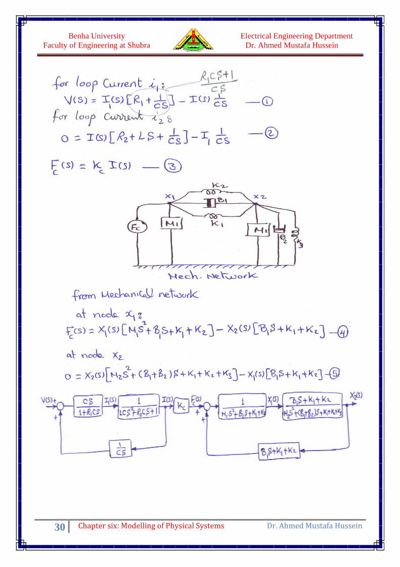
Example (17): For the electro-mechanical system shown below, the solenoid produces a magnetic

force FC = KC i. Draw the block diagram then find X2(s)/V(s)

M1

M2

K1 B

K2/2 K2/2

E

𝐾

1 + 𝑇𝑠

R1

C

R

Vo V1

f (t)

x1

x2

L



Benha University





Benha University



Sheet 5 (Physical Systems)

1) For the mechanical systems shown below;

• Draw the mechanical network, then write the system D.E’s

• If X2(s) is the system output, draw the block diagram and find X2(s)/F(s)



Benha University



2) Find the D.E’s that relates the distance X3 to 1 for the system shown below, then

draw the block diagram considering X3(s) as output. (the radius of the shaft is r).

3) For the mechanical systems shown below;

• Draw the mechanical network, then write the system D.E’s

• If 3(s) is the system output, draw the block diagram and find 3 (s)/T(s)



Benha University



4) For the mechanical system shown below, the solenoid produces a magnetic

force fc = Kc i. Draw the block diagram then find X(s)/V(s)

5) The mechanical system shown below is used to measuring the displacement x2

Write the D.E’s describing this system, then draw the block diagram.

6) For the system shown below, determine the closed loop T.F.



Benha University



7) For the motor-generator set shown below, the torque constant is KT for the

motor and KV for the generator. If the generator field current is assumed

constant, draw the block diagram then find the T.F. Y(s)/U(s).

8) For the separately-excited DC motor shown below, the torque-speed

characteristic is given by Tm = 200 - 8ωm. Draw the block diagram then find

the transfer function L(S)/Ea(S).

9) For the separately-excited DC motor shown below, the torque-speed

characteristic is given. Draw the block diagram then find the transfer function

L(S)/Ea(S).



Benha University



References:

[1] Bosch, R. GmbH. Automotive Electrics and Automotive Electronics, 5th ed. John Wiley & Sons

Ltd., UK, 2007.

[2] Franklin, G. F., Powell, J. D., and Emami-Naeini, A. Feedback Control of Dynamic Systems.

Addison-Wesley, Reading, MA, 1986.

[3] Dorf, R. C. Modern Control Systems, 5th ed. Addison-Wesley, Reading, MA, 1989.

[4] Nise, N. S. Control System Engineering, 6th ed. John Wiley & Sons Ltd., UK, 2011.

[5] Ogata, K. Modern Control Engineering, 5th ed ed. Prentice Hall, Upper Saddle River, NJ, 2010.

[6] Kuo, B. C. Automatic Control Systems, 5th ed. Prentice Hall, Upper Saddle River, NJ, 1987.

Benha University Faculty of Engineering at Shubra Dr ...

Documents

Transcript of Benha University Faculty of Engineering at Shubra Dr ...