
Bayesian Molecular Epidemiology - Page d'accueil / … Molecular Epidemiology Alexei Drummond,...
112
Bayesian Molecular Epidemiology Alexei Drummond, [email protected] Computational Evolution Group University of Auckland, Auckland, New Zealand May 21-25, MCEB, Montpellier 2013 1 / 112
Transcript of Bayesian Molecular Epidemiology - Page d'accueil / … Molecular Epidemiology Alexei Drummond,...

Bayesian Molecular Epidemiology
Alexei Drummond, [email protected] Evolution Group
University of Auckland, Auckland, New Zealand
May 21-25, MCEB, Montpellier 2013
1 / 112
Bayesian phylogenetics
Phylodynamics
Coalescent models
Birth-death-sampling models
Sampling ancestors
Structured tree models
Perspective
2 / 112
Acknowledgements
Phylodynamics@Computational EvolutionGroup
▶ Denise Kuhnert (PhDstudent)
▶ Jessie Wu (PhD student)▶ Sasha Gavryuskina (PhD
student)▶ Tim Vaughan (postdoc)▶ Remco Bouckaert
(postdoc)▶ Walter Xie (research
programmer)
Collaborators▶ Sebastian Bonhoeffer, ETH
Zurich▶ Tanja Stadler, ETH Zurich▶ Andrew Rambaut, Edinburgh, UK▶ Marc Suchard, UCLA▶ David Welch, Auckland, New
Zealand▶ Peter Drummond, SUT
Melbourne
3 / 112
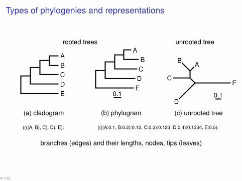
Types of phylogenies and representations
rooted trees unrooted tree..A.
B
.
C
.
D
.
E
(a) cladogram
..A .
B
.
C
.
D
.
E
.
0.1
(b) phylogram
..
A
.
B
.C .
D
. E.
0.1
(c) unrooted tree
((((A, B), C), D), E); ((((A:0.1, B:0.2):0.12, C:0.3):0.123, D:0.4):0.1234, E:0.5);
branches (edges) and their lengths, nodes, tips (leaves)
4 / 112
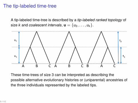
The tip-labeled time-tree
A tip-labeled time-tree is described by a tip-labeled ranked topology ofsize k and coalescent intervals, u = {u2, . . . , uk}.
These time-trees of size 3 can be interpreted as describing thepossible alternative evolutionary histories or (uniparental) ancestries ofthe three individuals represented by the labeled tips.
5 / 112
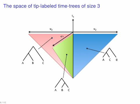
The space of tip-labeled time-trees of size 3
6 / 112
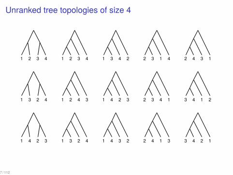
Unranked tree topologies of size 4
..1.
2.
3.
4.
1
.
3
.
2
.
4
.
1
.
4
.
2
.
3
.1
.2
.3
.4
.
1
.
2
.
4
.
3
.
1
.
3
.
2
.
4
.1
.3
.4
.2
.
1
.
4
.
2
.
3
.
1
.
4
.
3
.
2
.2
.3
.1
.4
.
2
.
3
.
4
.
1
.
2
.
4
.
1
.
3
.2
.4
.3
.1
.
3
.
4
.
1
.
2
.
3
.
4
.
2
.
1
7 / 112

How many trees are there?
For n species there are
Tn = 1 × 3 × 5 × · · · × (2n − 3) = (2n−3)!(n−2)!2n−2
rooted, tip-labelled binary trees:
n #trees4 15 enumerable by hand5 105 enumerable by hand on a rainy day6 945 enumerable by computer7 10395 still searchable very quickly on computer8 135135 about the number of hairs on your head9 2027025 greater than the population of Auckland10 34459425 ≈ upper limit for exhaustive search20 8.20 × 10²¹ ≈ upper limit of branch-and-bound searching48 3.21 × 1070 ≈ the number of particles in the Universe136 2.11 × 10267 number of trees to choose from in the “Out of Africa”
data (Vigilant et al. 1991)
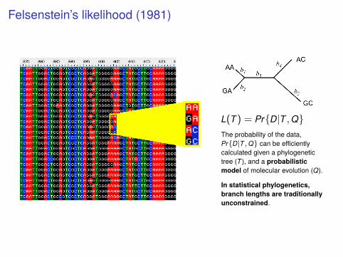
Felsenstein’s likelihood (1981)
L(T) = Pr{D|T ,Q}The probability of the data,Pr{D|T ,Q} can be efficientlycalculated given a phylogenetictree (T ), and a probabilisticmodel of molecular evolution (Q).
In statistical phylogenetics,branch lengths are traditionallyunconstrained.

Tree space as a hilly landscapeThe space of all possible trees can be visualized as a hilly landscape. Nearbypoints in this landscape represent similar trees, and the height of thelandscape is the probability of the tree at that point.
▶ This space can be sampled in a Bayesian analysis with MCMC
▶ The peak can be identified by a search algorithm in the context ofmaximum likelihoods
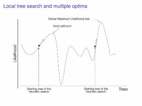
Local tree search and multiple optima
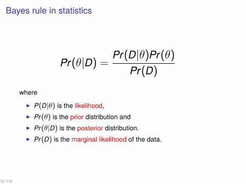
Bayes rule in statistics
Pr(θ|D) = Pr(D|θ)Pr(θ)Pr(D)
where
▶ P(D|θ) is the likelihood,▶ Pr(θ) is the prior distribution and▶ Pr(θ|D) is the posterior distribution.▶ Pr(D) is the marginal likelihood of the data.
12 / 112
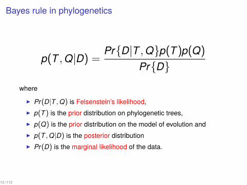
Bayes rule in phylogenetics
p(T ,Q|D) = Pr{D|T ,Q}p(T)p(Q)
Pr{D}
where
▶ Pr(D|T ,Q) is Felsenstein’s likelihood,▶ p(T) is the prior distribution on phylogenetic trees,▶ p(Q) is the prior distribution on the model of evolution and▶ p(T ,Q|D) is the posterior distribution▶ Pr(D) is the marginal likelihood of the data.
13 / 112
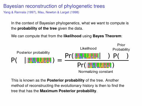
Bayesian reconstruction of phylogenetic treesYang & Rannala (1997), Mau, Newton & Larget (1998)
In the context of Bayesian phylogenetics, what we want to compute isthe probability of the tree given the data.
We can compute that from the likelihood using Bayes Theorem:
Pr( | )P( | ) =
Pr( )P( )|Likelihood
Posterior probability
Prior Probability
Normalizing constant
This is known as the Posterior probability of the tree. Anothermethod of reconstructing the evolutionary history is then to find thetree that has the Maximum Posterior probability.
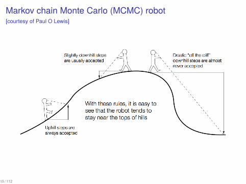
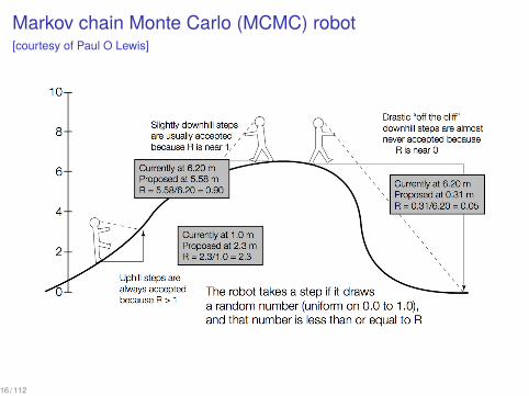
Markov chain Monte Carlo (MCMC) robot[courtesy of Paul O Lewis]
15 / 112
Markov chain Monte Carlo (MCMC) robot[courtesy of Paul O Lewis]
16 / 112
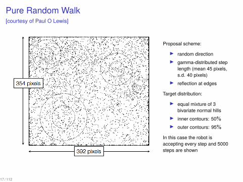
Pure Random Walk[courtesy of Paul O Lewis]
Proposal scheme:
▶ random direction▶ gamma-distributed step
length (mean 45 pixels,s.d. 40 pixels)
▶ reflection at edges
Target distribution:
▶ equal mixture of 3bivariate normal hills
▶ inner contours: 50%▶ outer contours: 95%
In this case the robot isaccepting every step and 5000steps are shown
17 / 112
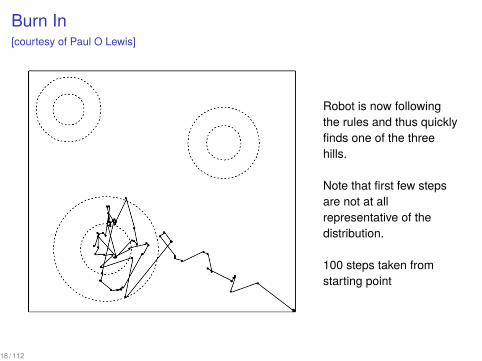
Burn In[courtesy of Paul O Lewis]
Robot is now followingthe rules and thus quicklyfinds one of the threehills.
Note that first few stepsare not at allrepresentative of thedistribution.
100 steps taken fromstarting point
18 / 112

Target Distribution Approximation[courtesy of Paul O Lewis]
How good is the MCMCapproximation?
▶ 51.2% of points areinside innercontours (cf. 50%actual)
▶ 93.6% of points areinside outercontours (cf. 95%actual)
Approximation getsbetter the longer thechain is allowed to run.
5000 steps taken
19 / 112

Target distribution versus proposal distribution
▶ The target distribution is the posterior distribution of interest▶ The proposal distribution is used to decide which point to try next
▶ you have much flexibility here, and the choice affects only theefficiency of the MCMC algorithm
▶ MCMC using a symmetric proposal distribution is the Metropolisalgorithm (Metropolis et al. 1953)
▶ Use of an asymmetric proposal distribution requires a modificationproposed by Hastings (1970), and is known as theMetropolis-Hastings algorithm
Metropolis, N., A. W. Rosenbluth, M. N. Rosenbluth, A. H. Teller, and E. Teller. 1953. Equation ofstate calculations by fast computing machines. J. Chem. Phys. 21:1087-1092.
20 / 112
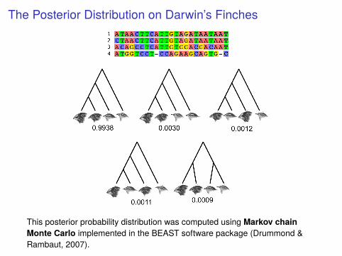
The Posterior Distribution on Darwin’s Finches
This posterior probability distribution was computed using Markov chainMonte Carlo implemented in the BEAST software package (Drummond &Rambaut, 2007).
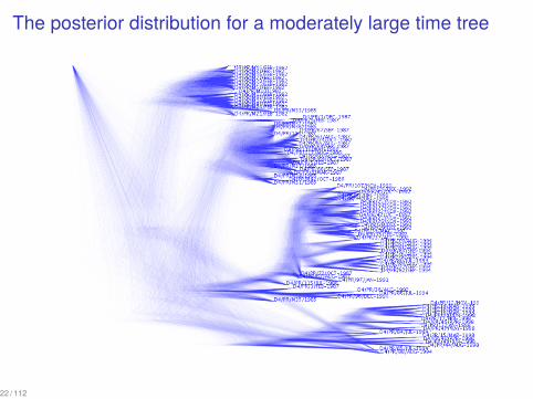
The posterior distribution for a moderately large time tree
22 / 112
..
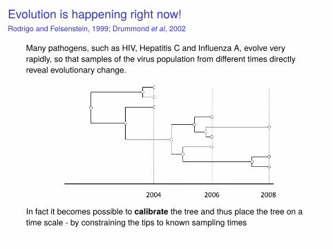
Evolution is happening right now!Rodrigo and Felsenstein, 1999; Drummond et al, 2002
Many pathogens, such as HIV, Hepatitis C and Influenza A, evolve veryrapidly, so that samples of the virus population from different times directlyreveal evolutionary change.
In fact it becomes possible to calibrate the tree and thus place the tree on atime scale - by constraining the tips to known sampling times
..
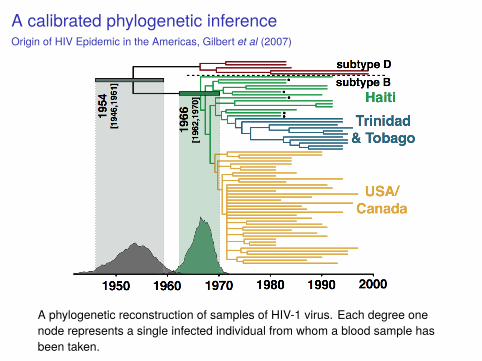
A calibrated phylogenetic inferenceOrigin of HIV Epidemic in the Americas, Gilbert et al (2007)
A phylogenetic reconstruction of samples of HIV-1 virus. Each degree onenode represents a single infected individual from whom a blood sample hasbeen taken.

Phylodynamics
▶ The intersection of phylogenetics and mathematicalepidemiology
▶ Includes estimation of epidemiological parameters fromphylogenetic data
▶ In a Bayesian setting, this has the familiar flavor of a hierarchicaltree prior
▶ The hyperparameters of the tree prior become dynamicalparameters of the epidemiological model
▶ The most common approach is to leverage coalescent theory, byusing coalescent machinery augmented with deterministic modelsof effective population size parametrized by R0 or itsepidemiological constituents (net infection rate et cetera).
27 / 112
Coalescent models

Bayesian coalescent inference
▶ Kingman’s coalescent is a mathematical theory describing agenealogy of a small random sample from a large backgroundpopulation.
▶ Provides a probability distribution over tree space given apopulation size history: P(G|N)
▶ Old coalescent trees come from large populations▶ Star-like coalescent trees come from exponentially growing
populations▶ In a Bayesian framework the coalescent is a hierarchical prior on
tree space.▶ Backwards in time model▶ Applied to both within-host and between-host population
dynamics
29 / 112

The coalescent with serial samplesMany epidemiological agents evolve very rapidly, so that the effect ofsampling the population at different times becomes important.
30 / 112
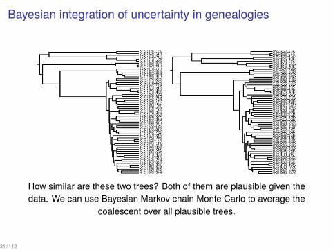
Bayesian integration of uncertainty in genealogies
How similar are these two trees? Both of them are plausible given thedata. We can use Bayesian Markov chain Monte Carlo to average the
coalescent over all plausible trees.
31 / 112
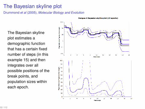
The Bayesian skyline plotDrummond et al (2005), Molecular Biology and Evolution
The Bayesian skylineplot estimates ademographic functionthat has a certain fixednumber of steps (in thisexample 15) and thenintegrates over allpossible positions of thebreak points, andpopulation sizes withineach epoch.
32 / 112
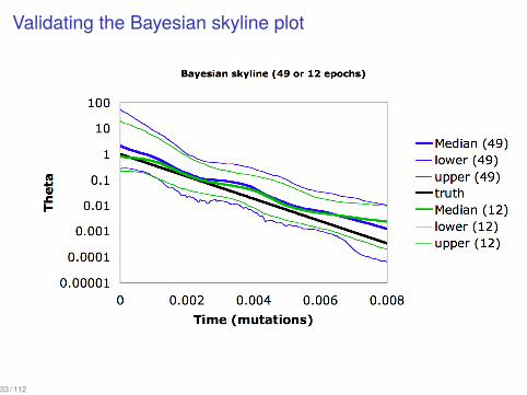
Validating the Bayesian skyline plot
33 / 112
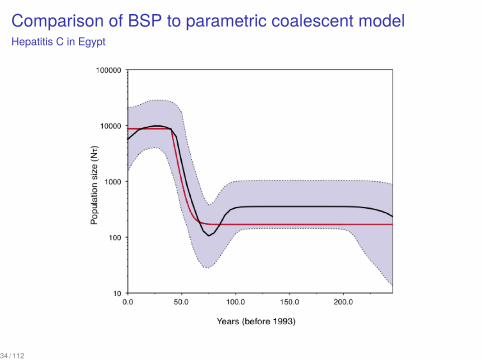
Comparison of BSP to parametric coalescent modelHepatitis C in Egypt
34 / 112
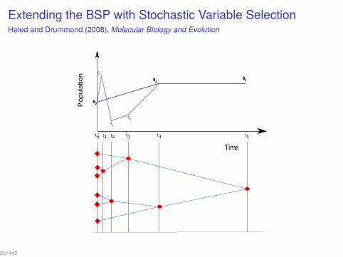
Extending the BSP with Stochastic Variable SelectionHeled and Drummond (2008), Molecular Biology and Evolution
35 / 112
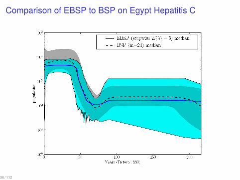
Comparison of EBSP to BSP on Egypt Hepatitis C
36 / 112
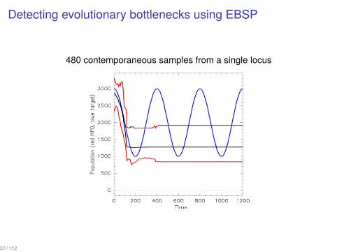
Detecting evolutionary bottlenecks using EBSP
480 contemporaneous samples from a single locus
37 / 112
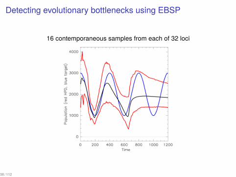
Detecting evolutionary bottlenecks using EBSP
16 contemporaneous samples from each of 32 loci
38 / 112
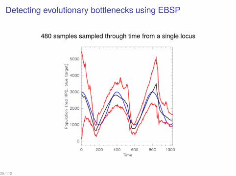
Detecting evolutionary bottlenecks using EBSP
480 samples sampled through time from a single locus
39 / 112

The population dynamics of genetic diversity in Influenza ARambaut et al (2008) Nature 453:615-620
40 / 112
Birth-death models
..
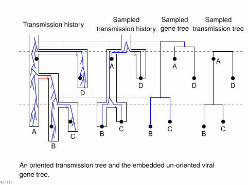
Transmission history
.....A
.
B
.
C
.
D
.
Sampled
.
transmission history
..B
.. C..
D
..
A
.
Sampled
.
gene tree
..B
.. C..
D
..
A
.
Sampled
.
transmission tree
..B
.. C..
D
..
A
An oriented transmission tree and the embedded un-oriented viralgene tree.
42 / 112
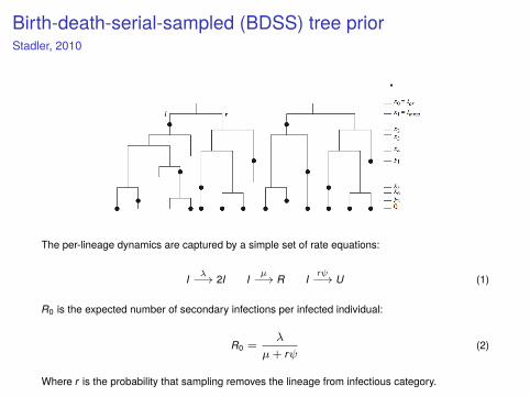
Birth-death-serial-sampled (BDSS) tree priorStadler, 2010
The per-lineage dynamics are captured by a simple set of rate equations:
I λ−→ 2I Iµ−→ R I
rψ−→ U (1)
R0 is the expected number of secondary infections per infected individual:
R0 =λ
µ+ rψ(2)
Where r is the probability that sampling removes the lineage from infectious category.
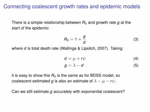
Connecting coalescent growth rates and epidemic models
There is a simple relationship between R0 and growth rate g at thestart of the epidemic:
R0 = 1 +gd
(3)
where d is total death rate (Wallinga & Lipsitch, 2007). Taking:
d = µ+ rψ (4)g = λ− d (5)
it is easy to show this R0 is the same as for BDSS model, socoalescent-estimated g is also an estimate of λ− µ− rψ.
Can we still estimate g accurately with exponential coalescent?
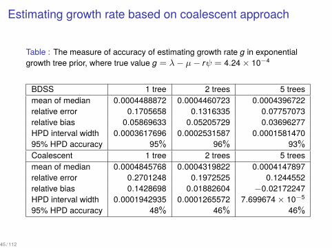
Estimating growth rate based on coalescent approach
Table : The measure of accuracy of estimating growth rate g in exponentialgrowth tree prior, where true value g = λ− µ− rψ = 4.24 × 10⁻⁴
BDSS 1 tree 2 trees 5 treesmean of median 0.0004488872 0.0004460723 0.0004396722relative error 0.1705658 0.1316335 0.07757073relative bias 0.05869633 0.05205729 0.03696277HPD interval width 0.0003617696 0.0002531587 0.000158147095% HPD accuracy 95% 96% 93%Coalescent 1 tree 2 trees 5 treesmean of median 0.0004845768 0.0004319822 0.0004147897relative error 0.2701248 0.1972525 0.1244552relative bias 0.1428698 0.01882604 −0.02172247HPD interval width 0.0001942935 0.0001265572 7.699674 × 10⁻⁵
95% HPD accuracy 48% 46% 46%
45 / 112
..
..
..

..
..
..

..
..
..
..
..
Sampling ancestors
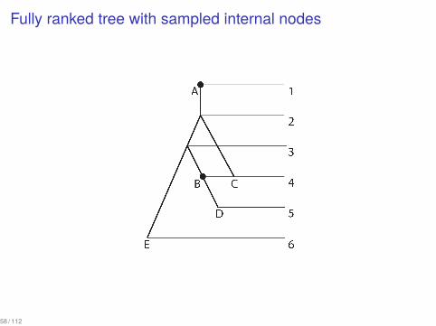
Fully ranked tree with sampled internal nodes
58 / 112
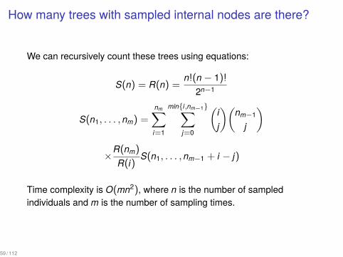
How many trees with sampled internal nodes are there?
We can recursively count these trees using equations:
S(n) = R(n) =n!(n − 1)!
2n−1
S(n1, . . . , nm) =nm∑i=1
min{i,nm−1}∑j=0
(ij
)(nm−1
j
)
×R(nm)
R(i)S(n1, . . . , nm−1 + i − j)
Time complexity is O(mn2), where n is the number of sampledindividuals and m is the number of sampling times.
59 / 112
Birth-death-sampling-through-time modelwith sampled ancestors
▶ birth rate λ▶ death rate µ▶ sampling rate ψ▶ become noninfectious probability r
This model produces only trees in which each sampled node hasdistinct rank.
60 / 112
Bayesian MCMC analysis with BEAST 2
Since this model produces trees which are not necessarily bifurcatingwe need to extend Bayesian MCMC methods and adapt BEAST 2 fordealing with a new type of tree.
▶ Prior distribution▶ Proposal mechanism▶ Likelihood (peeling algorithm)
61 / 112

Prior distribution
Stadler at el.:
f [T |λ, µ, ψ, r, tor = x0] = λm−1(ψ(1 − r))k
×m−1∏i=0
1q(xi)
m∏i=1
ψ(r + (1 − r)p0(yi))q(yi)
62 / 112
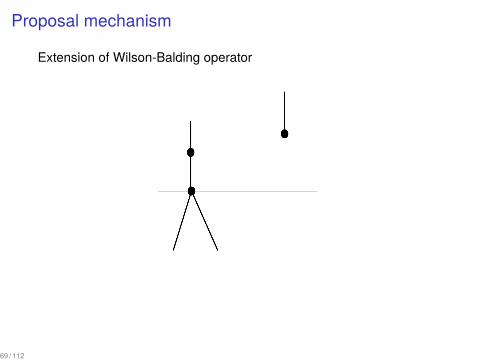
Proposal mechanism
An extension of Wilson-Balding operator
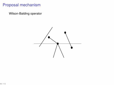
▶ Choose an edge ei that terminates at node i.▶ Choose an edge ej such that at least one end of ej is above i or a
leaf j which is above i excluding the edges adjacent to ei .▶ Prune the edge ei together with the descendant subtree and
attach it to the edge ej or to the leaf j.
63 / 112
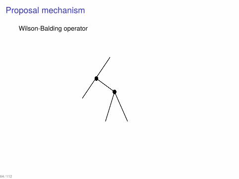
Proposal mechanism
Wilson-Balding operator
64 / 112
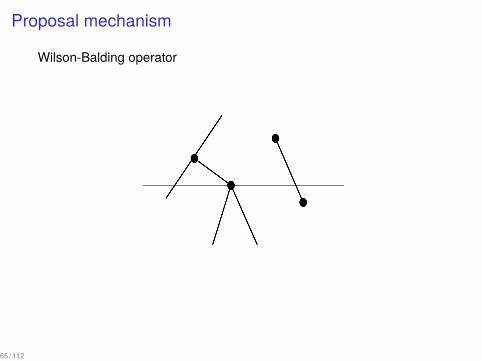
Proposal mechanism
Wilson-Balding operator
65 / 112
Proposal mechanism
Wilson-Balding operator
66 / 112
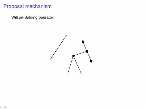
Proposal mechanism
Wilson-Balding operator
67 / 112
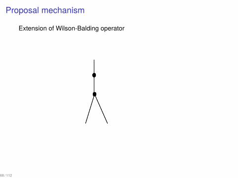
Proposal mechanism
Extension of Wilson-Balding operator
68 / 112
Proposal mechanism
Extension of Wilson-Balding operator
69 / 112

Proposal mechanism
Extension of Wilson-Balding operator
70 / 112
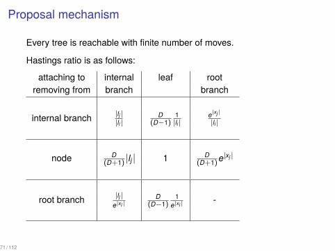
Proposal mechanism
Every tree is reachable with finite number of moves.
Hastings ratio is as follows:
attaching to internal leaf rootremoving from branch branch
internal branch |lj ||li |
D(D−1)
1|li |
e|xj |
|li |
node D(D+1) |lj | 1 D
(D+1)e|xj |
root branch |lj |e|xi |
D(D−1)
1e|xi |
-
71 / 112

Sampling from prior BEAST 2
λ = 2, µ = 1, ψ = 1, and r = 0.5.
6
y3 = 0
y2 = 1
y1 = 2
x0 = 3
•1
•2
•3
72 / 112
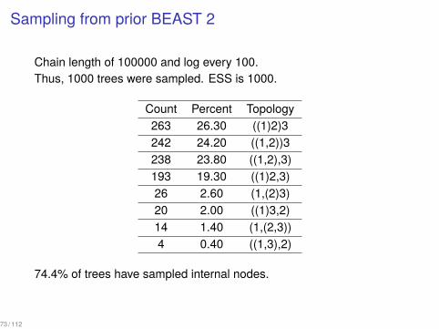
Sampling from prior BEAST 2
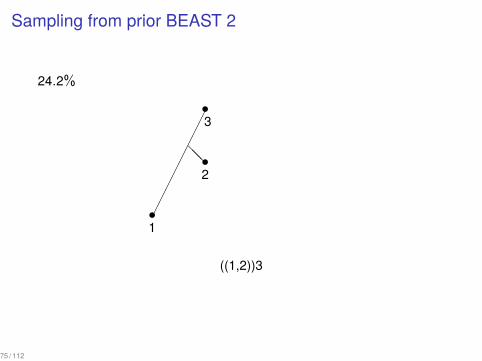
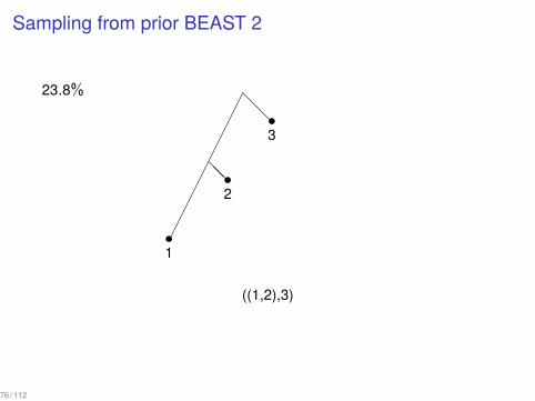
Chain length of 100000 and log every 100.Thus, 1000 trees were sampled. ESS is 1000.
Count Percent Topology263 26.30 ((1)2)3242 24.20 ((1,2))3238 23.80 ((1,2),3)193 19.30 ((1)2,3)26 2.60 (1,(2)3)20 2.00 ((1)3,2)14 1.40 (1,(2,3))4 0.40 ((1,3),2)
74.4% of trees have sampled internal nodes.
73 / 112
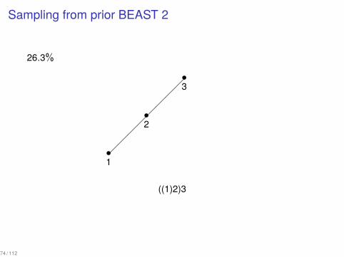
Sampling from prior BEAST 2
26.3%
•1
•2
•3
���
����
�
((1)2)3
74 / 112
Sampling from prior BEAST 2
24.2%
•1
•2
•3
��������
@@
((1,2))3
75 / 112
Sampling from prior BEAST 2
23.8%
•1
•2
•3
����������
@@
@@
((1,2),3)
76 / 112

Sampling from prior BEAST 2
19.3%
•1
•2
•3
����������
@@
((1)2,3)
77 / 112
Sampling from prior BEAST 2
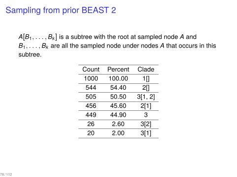
A[B1, . . . ,Bk] is a subtree with the root at sampled node A andB1, . . . ,Bk are all the sampled node under nodes A that occurs in thissubtree.
Count Percent Clade1000 100.00 1[]544 54.40 2[]505 50.50 3[1, 2]456 45.60 2[1]449 44.90 326 2.60 3[2]20 2.00 3[1]
78 / 112
Sampling from prior BEAST 2
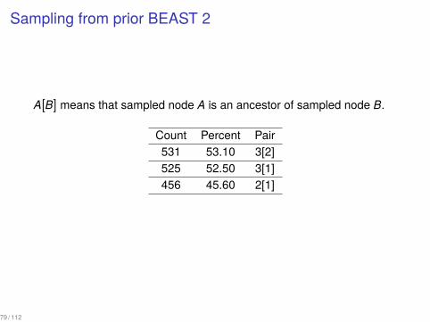
A[B] means that sampled node A is an ancestor of sampled node B.
Count Percent Pair531 53.10 3[2]525 52.50 3[1]456 45.60 2[1]
79 / 112
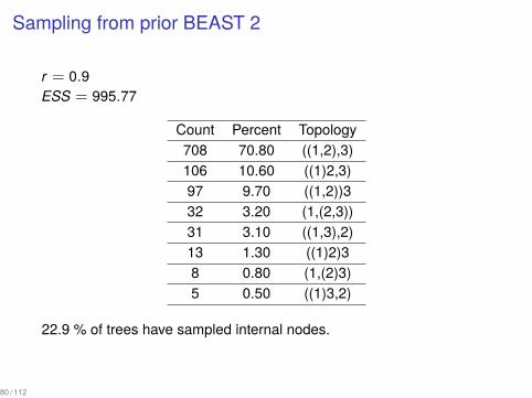
Sampling from prior BEAST 2
r = 0.9ESS = 995.77
Count Percent Topology708 70.80 ((1,2),3)106 10.60 ((1)2,3)97 9.70 ((1,2))332 3.20 (1,(2,3))31 3.10 ((1,3),2)13 1.30 ((1)2)38 0.80 (1,(2)3)5 0.50 ((1)3,2)
22.9 % of trees have sampled internal nodes.
80 / 112
Further work:
▶ Likelihood▶ More operators▶ Using other models, i.e. skyline model
81 / 112
Structured tree models
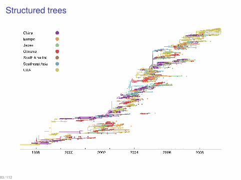
Structured trees
83 / 112
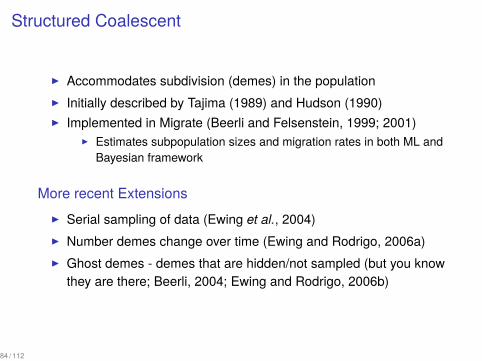
Structured Coalescent
▶ Accommodates subdivision (demes) in the population▶ Initially described by Tajima (1989) and Hudson (1990)▶ Implemented in Migrate (Beerli and Felsenstein, 1999; 2001)
▶ Estimates subpopulation sizes and migration rates in both ML andBayesian framework
More recent Extensions▶ Serial sampling of data (Ewing et al., 2004)▶ Number demes change over time (Ewing and Rodrigo, 2006a)▶ Ghost demes - demes that are hidden/not sampled (but you know
they are there; Beerli, 2004; Ewing and Rodrigo, 2006b)
84 / 112
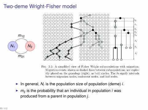
Two-deme Wright-Fisher model
..N1. N2.
m12
.
m21
▶ In general, Ni is the population size of population (deme) i.▶ mij is the probability that an individual in population i was
produced from a parent in population j.
85 / 112
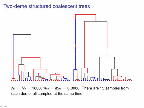
Two-deme structured coalescent trees...
N1 = N2 = 1000,m12 = m21 = 0.0008. There are 15 samples fromeach deme, all sampled at the same time.
86 / 112
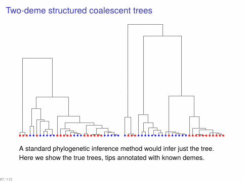
Two-deme structured coalescent trees...
A standard phylogenetic inference method would infer just the tree.Here we show the true trees, tips annotated with known demes.
87 / 112
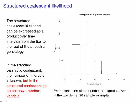
Structured coalescent likelihood
The structuredcoalescent likelihoodcan be expressed as aproduct over timeintervals from the tips tothe root of the ancestralgenealogy.
In the standardpanmictic coalescent,the number of intervalsis known, but in thestructured coalescent itsan unknown randomvariable.
Histogram of migration events
#migration events
Fre
quen
cy
0 10 20 30 40
010
020
030
040
0
Prior distribution of the number of migration eventsin the two deme, 30 sample example.
88 / 112

Bayesian MCMC of structured coalescent
In a non-structured Bayesian coalescent analysis, the tree topologyand coalescent times are sampled in a Markov chain of correlatedstates. The size of the discrete structure is fixed to n − 1 coalescentevents. Operators involve modifying the ancestral relationship treetopology or altering the times of the coalescent events.
For the structured coalescent we have to introduce new “operators”that can add or remove migration events to the ancestral history. Whena migration event is added it must be given a time and location on thetree. This increases the state space and thus the computationaldemand on the inference.
89 / 112

Beerli and Felsenstein (2001) proposal distribution
1. Tree proposals based on“dissolving” part of the tree andthen redrawing from the(conditional) prior.
2. Good at sampling from the prior3. Bad when the sequence data is
informative about the tree,because random coalescentsubtrees won’t fit the sequencedata well.
90 / 112
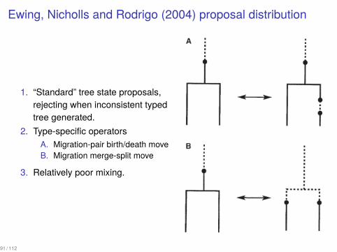
Ewing, Nicholls and Rodrigo (2004) proposal distribution
1. “Standard” tree state proposals,rejecting when inconsistent typedtree generated.
2. Type-specific operatorsA. Migration-pair birth/death moveB. Migration merge-split move
3. Relatively poor mixing.
91 / 112

Operator design strategy
With some exceptions, we take the following general approach tooperator development.
▶ Apply a standard tree move paying noattention to types.
▶ Type-changes along altered branches areregenerated.
▶ Regeneration is accomplished by drawingnew migration paths from a continuous timeMarkov process generated by the currentrate matrix conditional on types at each endof the branch.
.
92 / 112

Operator design strategy
With some exceptions, we take the following general approach tooperator development.
▶ Apply a standard tree move paying noattention to types.
▶ Type-changes along altered branches areregenerated.
▶ Regeneration is accomplished by drawingnew migration paths from a continuous timeMarkov process generated by the currentrate matrix conditional on types at each endof the branch.
.
93 / 112
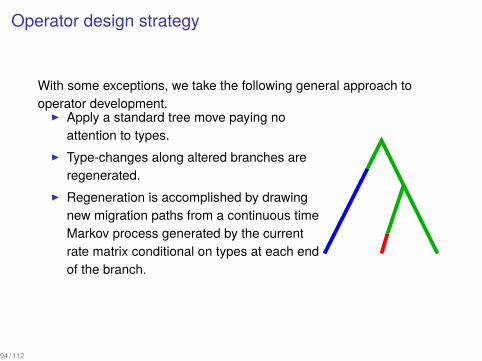
Operator design strategy
With some exceptions, we take the following general approach tooperator development.
▶ Apply a standard tree move paying noattention to types.
▶ Type-changes along altered branches areregenerated.
▶ Regeneration is accomplished by drawingnew migration paths from a continuous timeMarkov process generated by the currentrate matrix conditional on types at each endof the branch.
.
94 / 112
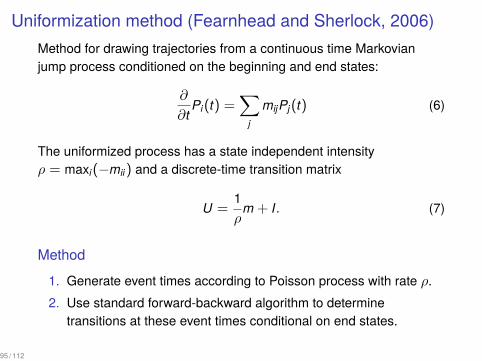
Uniformization method (Fearnhead and Sherlock, 2006)Method for drawing trajectories from a continuous time Markovianjump process conditioned on the beginning and end states:
∂
∂tPi(t) =
∑j
mijPj(t) (6)
The uniformized process has a state independent intensityρ = maxi(−mii) and a discrete-time transition matrix
U =1ρ
m + I. (7)
Method1. Generate event times according to Poisson process with rate ρ.2. Use standard forward-backward algorithm to determine
transitions at these event times conditional on end states.
95 / 112
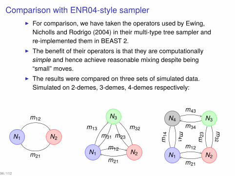
Comparison with ENR04-style sampler▶ For comparison, we have taken the operators used by Ewing,
Nicholls and Rodrigo (2004) in their multi-type tree sampler andre-implemented them in BEAST 2.
▶ The benefit of their operators is that they are computationallysimple and hence achieve reasonable mixing despite being“small” moves.
▶ The results were compared on three sets of simulated data.Simulated on 2-demes, 3-demes, 4-demes respectively:
..N1. N2.
m12
.
m21..N1. N2.
N3
. m12.
m13
.m21
.
m23
.
m31
.
m32
..N1. N2.
N3
.
N4
.m12
.m
14
.m21
.
m23
.
m32
.
m34
.
m41
.
m43
96 / 112
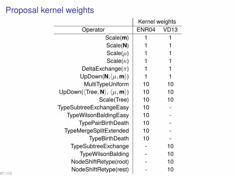
Proposal kernel weightsKernel weights
Operator ENR04 VD13Scale(m) 1 1Scale(N) 1 1Scale(µ) 1 1Scale(κ) 1 1
DeltaExchange(π) 1 1UpDown(N,⟨µ,m⟩) 1 1
MultiTypeUniform 10 10UpDown(⟨Tree,N⟩, ⟨µ,m⟩) 10 10
Scale(Tree) 10 10TypeSubtreeExchangeEasy 10 -
TypeWilsonBaldingEasy 10 -TypePairBirthDeath 10 -
TypeMergeSplitExtended 10 -TypeBirthDeath 10 -
TypeSubtreeExchange - 10TypeWilsonBalding - 10
NodeShiftRetype(root) - 10NodeShiftRetype(rest) - 10
97 / 112
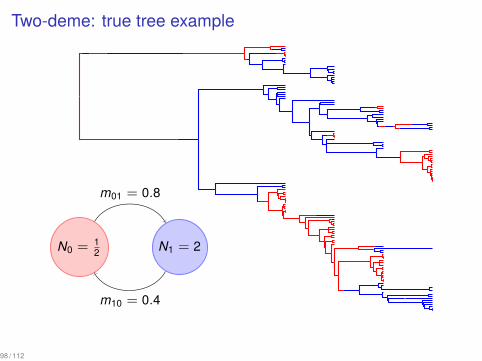
Two-deme: true tree example...
N0 = 12
.
N1 = 2
.
m01 = 0.8
.
m10 = 0.4
98 / 112
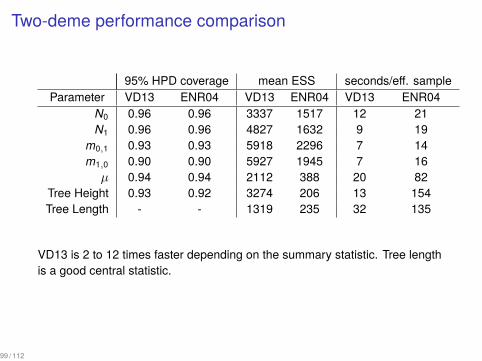
Two-deme performance comparison
95% HPD coverage mean ESS seconds/eff. sampleParameter VD13 ENR04 VD13 ENR04 VD13 ENR04
N0 0.96 0.96 3337 1517 12 21N1 0.96 0.96 4827 1632 9 19
m0,1 0.93 0.93 5918 2296 7 14m1,0 0.90 0.90 5927 1945 7 16µ 0.94 0.94 2112 388 20 82
Tree Height 0.93 0.92 3274 206 13 154Tree Length - - 1319 235 32 135
VD13 is 2 to 12 times faster depending on the summary statistic. Tree lengthis a good central statistic.
99 / 112
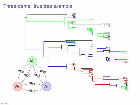
Three-deme: true tree example...
N0
.
N1
.
N2
.
m01
.
m02
.
m10
.
m12
.
m20
.
m21
100 / 112
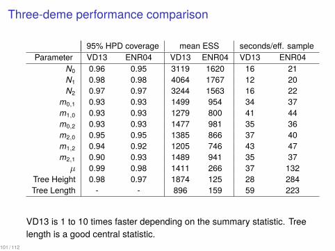
Three-deme performance comparison
95% HPD coverage mean ESS seconds/eff. sampleParameter VD13 ENR04 VD13 ENR04 VD13 ENR04
N0 0.96 0.95 3119 1620 16 21N1 0.98 0.98 4064 1767 12 20N2 0.97 0.97 3244 1563 16 22
m0,1 0.93 0.93 1499 954 34 37m1,0 0.93 0.93 1279 800 41 44m0,2 0.93 0.93 1477 981 35 36m2,0 0.95 0.95 1385 866 37 40m1,2 0.94 0.92 1205 746 43 47m2,1 0.90 0.93 1489 941 35 37µ 0.99 0.98 1411 266 37 132
Tree Height 0.98 0.97 1874 125 28 284Tree Length - - 896 159 59 223
VD13 is 1 to 10 times faster depending on the summary statistic. Treelength is a good central statistic.
101 / 112

Four-deme: true tree example...
N1
.
N2
.
N3
.
N4
.
m12
.
m14
.
m21
.
m23
.
m32
.
m34
.
m41
.
m43
102 / 112
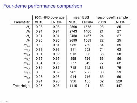
Four-deme performance comparison
95% HPD coverage mean ESS seconds/eff. sampleParameter VD13 ENR04 VD13 ENR04 VD13 ENR04
N0 0.96 0.96 2560 1578 23 25N1 0.94 0.94 2743 1486 21 27N2 0.91 0.91 2458 1467 24 27N3 0.95 0.95 2699 1569 22 25
m0,3 0.80 0.81 935 739 64 55m0,1 0.93 0.93 811 652 74 62m2,1 0.91 0.92 913 693 65 58m3,0 0.95 0.95 898 726 66 56m1,0 0.84 0.85 777 649 77 62m1,2 0.84 0.85 718 542 83 75m3,2 0.88 0.89 901 756 66 53m2,3 0.93 0.93 914 716 65 56µ 0.94 0.93 956 185 62 220
Tree Height 0.95 0.96 1115 91 53 447
103 / 112

Multi-type birth-death processAssume that the process is started with one infected individual indeme or of type i ∈ {1 . . . d} at time t = 0. With time increasing fromthe past to the present, in a time step ∆t the process can undergo
1. a birth event, so that another infected individual is created indeme i:
Ni(t +∆t) = Ni(t) + 1,
2. a death event, implying the recovery or removal of an infectedindividual in deme i:
Ni(t +∆t) = Ni(t)− 1,
3. a sampling event, yielding the removal of an infected individual asin 2., but this time the removal is observed, or
4. a migration event, indicating that an individual changes fromdeme i to deme j ̸= i:
Ni(t +∆t) = Ni(t)− 1 and Nj(t +∆t) = Nj(t) + 1.
The process terminates when no infected individuals are left.104 / 112
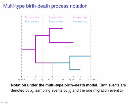
Multi-type birth-death process notation
t0 = 0
λ1,1, µ1,1, ψ1,1
λ2,2, µ2,2, ψ2,2
t1
λ1,2, µ1,2, ψ1,2
λ2,2, µ2,2, ψ2,2
t2
λ1,3, µ1,3, ψ1,3
λ2,3, µ2,3, ψ2,3
tm = y4y1 y2 y3x1 x2 z1
1
Notation under the multi-type birth–death model. Birth events aredenoted by xj , sampling events by yj and the one migration event z1.
105 / 112
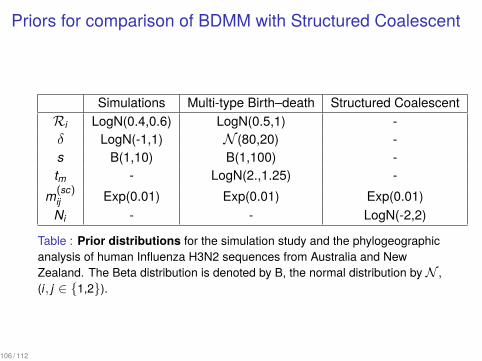
Priors for comparison of BDMM with Structured Coalescent
Simulations Multi-type Birth–death Structured CoalescentRi LogN(0.4,0.6) LogN(0.5,1) -δ LogN(-1,1) N (80,20) -s B(1,10) B(1,100) -tm - LogN(2.,1.25) -
m(sc)ij Exp(0.01) Exp(0.01) Exp(0.01)Ni - - LogN(-2,2)
Table : Prior distributions for the simulation study and the phylogeographicanalysis of human Influenza H3N2 sequences from Australia and NewZealand. The Beta distribution is denoted by B, the normal distribution by N ,(i, j ∈ {1,2}).
106 / 112
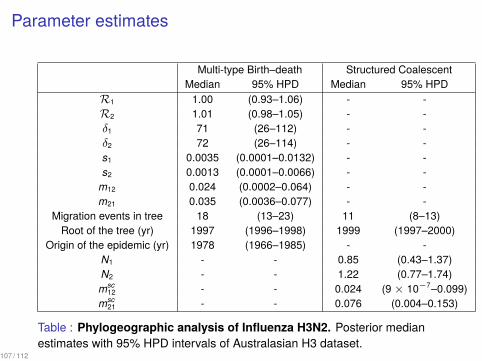
Parameter estimates
Multi-type Birth–death Structured CoalescentMedian 95% HPD Median 95% HPD
R1 1.00 (0.93–1.06) - -R2 1.01 (0.98–1.05) - -δ1 71 (26–112) - -δ2 72 (26–114) - -s1 0.0035 (0.0001–0.0132) - -s2 0.0013 (0.0001–0.0066) - -
m12 0.024 (0.0002–0.064) - -m21 0.035 (0.0036–0.077) - -
Migration events in tree 18 (13–23) 11 (8–13)Root of the tree (yr) 1997 (1996–1998) 1999 (1997–2000)
Origin of the epidemic (yr) 1978 (1966–1985) - -N1 - - 0.85 (0.43–1.37)N2 - - 1.22 (0.77–1.74)msc
12 - - 0.024 (9 × 10⁻⁷–0.099)msc
21 - - 0.076 (0.004–0.153)
Table : Phylogeographic analysis of Influenza H3N2. Posterior medianestimates with 95% HPD intervals of Australasian H3 dataset.
107 / 112
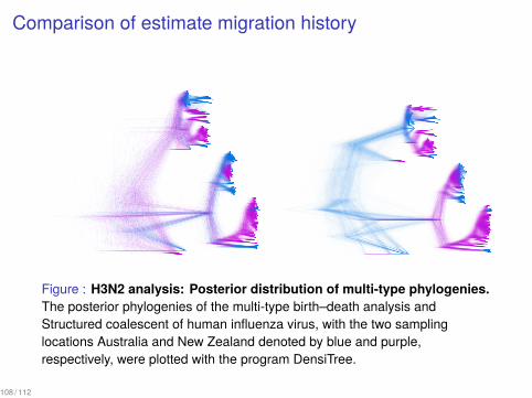
Comparison of estimate migration history
Figure : H3N2 analysis: Posterior distribution of multi-type phylogenies.The posterior phylogenies of the multi-type birth–death analysis andStructured coalescent of human influenza virus, with the two samplinglocations Australia and New Zealand denoted by blue and purple,respectively, were plotted with the program DensiTree.
108 / 112
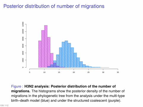
Posterior distribution of number of migrations
5 10 15 20 25 30 35
020
0040
0060
0080
0010
000
1200
0
Figure : H3N2 analysis: Posterior distribution of the number ofmigrations. The histograms show the posterior density of the number ofmigrations in the phylogenetic tree from the analysis under the multi-typebirth–death model (blue) and under the structured coalescent (purple).
109 / 112
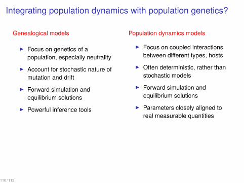
Integrating population dynamics with population genetics?
Genealogical models
▶ Focus on genetics of apopulation, especially neutrality
▶ Account for stochastic nature ofmutation and drift
▶ Forward simulation andequilibrium solutions
▶ Powerful inference tools
Population dynamics models
▶ Focus on coupled interactionsbetween different types, hosts
▶ Often deterministic, rather thanstochastic models
▶ Forward simulation andequilibrium solutions
▶ Parameters closely aligned toreal measurable quantities
110 / 112
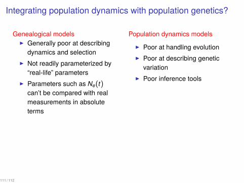
Integrating population dynamics with population genetics?
Genealogical models▶ Generally poor at describing
dynamics and selection▶ Not readily parameterized by
“real-life” parameters▶ Parameters such as Ne(t)
can’t be compared with realmeasurements in absoluteterms
Population dynamics models
▶ Poor at handling evolution▶ Poor at describing genetic
variation▶ Poor inference tools
111 / 112

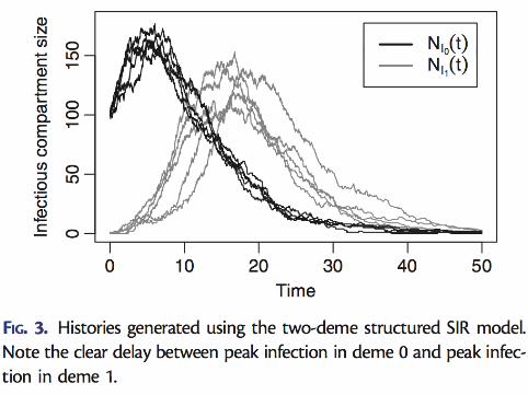
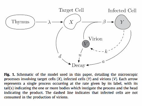
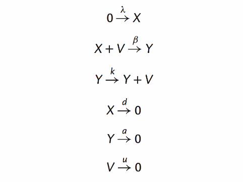
Dynamical population geneticsWhat would a synthesis look like?
▶ Microscopic descriptions of all processes including▶ Selection, competition▶ Mutation, type switching▶ Birth, death, infection, genetic drift et cetera▶ Demographic stochasticity▶ Environmental stochasticity
▶ Natural modeling of stochastic parts of the process▶ Retains non-linear coupling between different types and hosts▶ Handles both neutral and selected variation▶ Parameters can be readily connected with real measurable
quantities▶ Simulation, analysis and inference tools
112 / 112