Are You suprised - scu.ac.ir
88
Transcript of Are You suprised - scu.ac.ir

AUTUMN 2016, Vol II, No II, JOURNAL OF HYDRAULIC STRUCTURES
JORNAL OF
HYDRAULIC STRUCTURES SHAHID CHAMRAN UNIVERSITY OF AHVAZ
Manager: Prof. Hamid R. Ghafouri
Editor-in-chief: Dr. Ali Haghighi Editorial coordinator: Dr. Seyed Mohammad Ashrafi
Department of Civil Engineering, Engineering Faculty, Shahid Chamran University of Ahvaz, Ahvaz, Iran. Members Prof. Hossein M. V.Samani Civil Engineering Department, Shahid Chamran University of Ahvaz, Ahvaz, Iran Prof. Hamid R. Ghafouri Civil Engineering Department, Shahid Chamran University of Ahvaz, Ahvaz, Iran
Prof. Mohammad M. Shooshtari Civil Engineering Department, Shahid Chamran University of Ahvaz, Ahvaz, Iran
Prof. Mahmood S. Bajestan Hydraulic Structures Department, Shahid Chamran University of Ahvaz, Ahvaz, Iran
Prof. Saeed R. S. Yazdi Civil Engineering Department, K.N.Toosi University of Technology, Tehran, Iran
Prof. Ahmadreza M. Gharabaghi Civil Engineering Faculty, Sahand University of Technology, Tabriz, Iran
Prof. Behzad Ataie Ashtiani Civil Engineering Department, Sharif University of Technology, Tehran, Iran
Prof. Masoud Ghodsian Faculty of Civil & Environmental Engineering, TarbiatModarres University, Tehran, Iran
Prof. Mahmood Javan School of Agriculture Shiraz University, Shiraz, Iran
Prof. Javad Farhoudi Department of Irrigation & Reclamation Engineering University of Tehran, Tehran, Iran
Prof. Mohammad R. Jaefarzadeh Department of Civil Engineering, Ferdowsi University, Mashhad, Iran
Prof. Nasser Talebbeydokhti Department of Civil Engineering, Shiraz University, Shiraz, Iran
Dr. Mohammad S. Pakbaz Civil Engineering Department, Shahid Chamran University of Ahvaz, Ahvaz, Iran
Dr. Massoud Oulapour Civil Engineering Department, Shahid Chamran University of Ahvaz, Ahvaz, Iran
Dr. Arash Adib Civil Engeering Department, Shahid Chamran University of Ahvaz, Ahvaz, Iran
Dr. Ali Haghighi Civil Engineering Department, Shahid Chamran University of Ahvaz, Ahvaz, Iran
Dr. Mojtaba Labibzadeh Civil Engineering Department, Shahid Chamran University of Ahvaz, Ahvaz, Iran
CONTENTS VOL II, NO II, AUTUMN 2016
II Aims and Scope
01 Groundwater Level Forecasting Using Wavelet and Kriging T. Rajaee, V. Nourani, F. Pouraslan
22 Numerical investigation of free surface flood wave and solitary wave using incompressible SPH method M. Zounemat-Kermani, H. Sheybanifard
35 Hydrological Assessment of Daily Satellite Precipitation Products over a Basin in Iran S. Moazami, A. Abdollahipour, M.Z. Niri, S.M. Ashrafi
46 Numerical Simulation of Flow Pattern around the Bridge Pier with Submerged Vanes S. Haji Azizi, D. Farsadizadeh, H. Arvanaghi, A. Abbaspour
62 Flood Forecasting Using Artificial Neural Networks: an Application of Multi-Model Data Fusion Technique Y. Tahmasebi Biragani, F. Yazdandoost, H. Ghalkhani
74 Estimation of Sediment Transport Rate of Karun River (Iran) N. Najafpoura, S. Emamgholizadeh, H.Torabi poudeh, A. H. Haghiabi

AUTUMN 2016, Vol II, No II, JOURNAL OF HYDRAULIC STRUCTURES
Aims and Scope Hydraulic Structure Journal is an interdisciplinary journal which publishes high-quality peer-
reviewed articles addressing the latest developments and applied methods in construction,
maintenance, management, and operation policy of Hydraulic Structures.
The Journal aims at providing an efficient route to fast-track publication, within 10-12 weeks
after manuscript submission. Manuscripts will be considered for publication in the following
categories: research articles, technical notes, case reports and discussions.
The general areas covered by the Journal include:
Technical and methodological advances in application, design/selection, production,
modification of construction materials
Advances in numerical and analytical methods
Hydro informatics and soft computing
Hydraulic aspects of hydraulic structures
Applied surface and subsurface hydrology and hydrometeorology
Forecasting approaches in water resources engineering
Economic and social aspects of hydraulic structures
Uncertainty analysis and risk management in hydraulics and water resources engineering
Application of Nanotechnology in Hydraulic Structures
Geotechnics of Hydraulic Structures
Damage detection techniques
The following might be considered as hydraulic structures:
Dams and associated structures
River and Watershed Structures
Offshore and Onshore Structures
Irrigation and Drainage Channel Networks
Bridges
Water Storage and Conveyance Structures
Pipelines and Pump Stations
Sewerage Systems
Water and Wastewater Treatment Plants
Historical Water Structures
General Information
Title: Journal of Hydraulic Structures
Subject: Hydraulics and water resources engineering
Coverage area: International
Journal Type: Scientific and technical
License Holder: Shahid Chamran University
Editor-in-Chief: Dr. Ali Haghighi
Manager: Prof. Hamid R. Ghafouri
Editorial coordinator: Dr. Seyed Mohammad Ashrafi
Language Editors: Majid SadollahKhani
Soroosh Kamali
Address: Engineering Faculty,
Shahid Chamran University of
Ahvaz
Phone #: +986113330010-20
(5610 & 5603)
Fax #: +986113337010
Language: English
Email: [email protected]
Website: jhs.scu.ac.ir
AUTUMN 2016, Vol II, No II, JOURNAL OF HYDRAULIC STRUCTURES
Shahid Chamran University of Ahvaz
Journal of Hydraulic Structures
J. Hydraul. Struct., 2016; 2(2):1-21
DOI: 10.22055/jhs.2016.12848
Groundwater Level Forecasting Using Wavelet and Kriging
Taher Rajaee1
Vahid Nourani 2
Fatemeh Pouraslan3
Abstract In this research, a hybrid wavelet-artificial neural network (WANN) and a geostatistical method
were proposed for spatiotemporal prediction of the groundwater level (GWL) for one month
ahead. For this purpose, monthly observed time series of GWL were collected from September
2005 to April 2014 in 10 piezometers around Mashhad City in the Northeast of Iran. In temporal
forecasting, an artificial neural network (ANN) and a WANN were trained for each piezometer.
Kriging was used in spatial estimations. The comparison of the prediction accuracy of these two
models illustrated that the WANN was more efficacious in prediction of GWL for one month
ahead. Thereafter, in order to predict GWL in desired points in the study area, the kriging
method was used and a Gaussian model was selected as the best variogram model. Ultimately,
the WANN with coefficient of determination and root mean square error and mean absolute
error, 0.836 and 0.335 and 0.273 respectively, in temporal forecasting and Gaussian model with
root mean square, 0.253 as the best fitted model on Kriging method for spatial estimating were
suitable choices for spatiotemporal GWL forecasting. The obtained map of groundwater level
showed that the groundwater level was higher in the areas of plain located in mountainside areas.
This fact can show that outcomes are respectively correct.
Keywords: Artificial neural network, wavelet, kriging, spatiotemporal prediction, groundwater
level
Received: 15 September 2016; Accepted: 20 November 2016
1. Introduction
Most areas of the world are categorized as warm and arid areas; therefore, given the lack of
precipitation and surface water, potable water and/or agricultural waters are only restricted to
1Associate Professor, Department of Civil Eng., University of Qom, Qom, Iran, E-mail addresses:
[email protected]; [email protected]. 2 Professor, Department of Water Resources Engineering, Faculty of Civil Engineering, University of
Tabriz, Tabriz, Iran. E-mail addresses: [email protected]. 3 M.Sc. in Hydraulic Structures, Department of Civil Eng., University of Qom, Qom, Iran, E-mail
addresses: [email protected]
T. Rajaee, V. Nourani, F. Pouraslan
AUTUMN 2016, Vol II, No II, JOURNAL OF HYDRAULIC STRUCTURES
Shahid Chamran University of Ahvaz
2
groundwater resources. The prediction of GWL is a complex phenomenon and usually needs a
lot of data and a long response time. Prediction of GWL is important for effective management
of GWL such as aquifer development, contaminated remediation aquifer or performance
assessment of planned water supply projects. Studies have been conducted to reduce the
complexities of the problem in terms of developing practical techniques that do not require
dwelling on algorithms and theories (Rajaee., 2011). Numerous studies with many methods and
models for modelling of GWL have been reported, which are based on various theories (Yang et
al., 2009; Shiri & Kisi, 2011; Yoon et al., 2011; Mohammadi, 2008; Nourani et al., 2011). One
of these physical theories is based on numerical models that establish a governing equation
simplifying the physics of flow in the subsurface and solve it with proper initial and boundary
conditions (Yoon et al., 2011). This model requires various hydrological and geological patterns
(Nakhaee & Saberinasr., 2012). The other models for prediction of GWL such as the Time
Series model, the integrated time series model (Yang et al., 2009), autoregressive moving
average model (Zhou et al., 2008; Kisi, 2010), the seasonal autoregressive moving average
model (Gemitzi & Stefanopoulos, 2011; Zhou et al., 2008), the periodic autoregressive model,
and the threshold autoregressive model (Wang et al., 2009) have been suggested in the past
decades.
In the field of water resources and environmental engineering, artificial neural network
(ANN) models have recently been applied to contamination modelling in shallow groundwaters
(Sahoo et al., 2006), studying the ANN model for prediction of suspended sediment
concentration (SSC) belonging to rivers (Rajaee et al., 2009) and forecasting the ozone episode
days (Tsai et al., 2009). The ANN was used by Aziz & Wong (1992) to estimate aquifer
parameters of groundwater. Lallahem et al (2005) used ANN to assess water tables in fractured
media. Daliakopoulos et al (2005) investigated seven different types of network architectures
and training algorithms for GWL forecasting in Messara valley with a neural network. The
experiment results showed that a standard feed forward neural network trained with the
Levenberg-Marquardt algorithm provided the best result. Nourani et al. (2008) evaluated the
feasibility of using an ANN methodology for estimating the GWLs. The efficiency of the spatio-
temporal ANN (STANN) model has beem compared with two hybrid neural-geostatistics (NG)
and multivariate time series-geostatistics (TSG) models. The results showed that the ANNs
provided the most accurate predictions in comparison with the other models. In a comparative
assessment, Sahoo & Jha (2013) concluded that the ANN technique was superior to the multiple
linear regression (MLR) technique in predicting the spatio-temporal distribution of the
groundwater levels in a basin. In another research, Maiti & Tiwari (2014) compared the ANNs,
the Bayesian neural networks and the adaptive neuro-fuzzy inference system (ANFIS) in GWL
prediction. The results showed that the Bayesian neural networks (BNN) optimized by SCG
models performed better than both the ANFIS and ANN optimized by a scaled conjugate
gradient (SCG) (ANN.SCG).
If the input data are non-stationary, the accuracy of the neural networks decreases. One of the
methods proposed to resolve this subject was wavelet analysis which has been applied to a
number of problems in water resources and environmental engineering such as river flow
modelling (Pasquini & Depetris, 2007). A non-stationary signal can be decomposed into a
certain number of stationary signals by a wavelet transform. Then ANN is combined with the
wavelet transform to improve the prediction accuracy (Zhou et al., 2008). Rajaee (2010)
proposed a model by combining the wavelet analysis and neuro-fuzzy approach to predict the
daily suspended sediments.
Wavelet analysis, which provides information in both time and frequency domains of the
Groundwater Level Forecasting Using Wavelet and Kriging
AUTUMN 2016, Vol II, No II, JOURNAL OF HYDRAULIC STRUCTURES
Shahid Chamran University of Ahvaz
3
signal, gives considerable insight into the physical form of the data. Using hybrid wavelet-ANN
(WANN) model to predict natural phenomena is a new method. Shoaib et al (2014) compared
different wavelet-based neural network models for the rainfall-runoff modelling. Nourani et al
(2014) focused on defining hybrid modelling. They explained advantages of such combined
models, as well as the history and potential future of their application in hydrology to predict
important processes of the hydrologic cycle. Adamowski & chen (2011) have shown that the
combined model is much more precise than classical models like ANN and autoregressive
integrated moving average (ARMIA). Nakhaee & Saberinasr (2012) used combined the
Wavelet-ANN model and its application in prediction of GWL fluctuations. For a better and
more precise analysis, the forecasted results of the model were compared with the observed data
not only in the validation stage but also in the test stage. Nourani et al (2009) used a combined
neural-wavelet model for prediction of Ligvanchai watershed precipitation and the obtained
results showed that the proposed model could predict both short- and long-term precipitation
events.
A very useful tool for a precise and detailed study to elucidate the behaviour of GWL
fluctuations in both spatial and temporal scales is geostatistics (Rouhani & Wackernagel, 1990).
Reghunath et al., (2005) and Kumar et al (2005) have emphasized the use of geostatistics for a
better management and conservation of water resources and sustainable development of any
area. They have reported that geostatistical methods are good tools for water resources
management and can be effectively used to derive the long-term trends of a groundwater.
Abedian et al (2013) used a geostatistical method. They optimized monitoring network of water
tables by geostatistical methods. In designing such a network, it is necessary to pay attention to
the distribution of variables all over the aquifer so that variables represent a whole picture of the
aquifer correctly. Using geostatistical methods, a water table network was optimized for the
aquifer. At the end of this study, the network was optimized by deleting a piezometer and adding
two other ones. Kholgi & Hosseini (2009) investigated in interpolation of GWL in an
unconfined aquifer in the north of Iran using Neuro-fuzzy and Ordinary Kriging.
The current research is a new application of Wavelet-ANN-Kriging hybrid model which at
first uses a multi-scale signal for prediction of GWL in ten piezometers for one step later inside
and environs of Mashhad City in Iran, and interpolation of GWL in places where there is not any
piezometer, especially in areas of city where the construction of a piezometer is not possible.
The rest of the paper is organized as follows. The location of the piezometer and statistical
analysis are presented in Section 2. The methods used in this study are proposed in Section 3.
Section 4 presents the model application for a real world problem. The results and discussion are
presented in Section 5. Summary and conclusion will be the topics of Section 6.
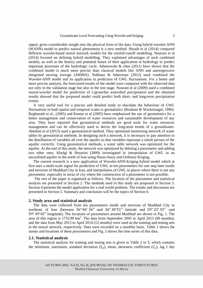
2. Study area and statistical analysis The data were collected from ten piezometers inside and environs of Mashhad City in
northeast of Iran (between 36° 06′ 36′′ -and 36° 30′51′′ -latitude and 59° 23′ 33′′ -and
59° 49′45′′ longitude). The locations of piezometers around Mashhad are shown in Fig. 1. The
area of this region is 1753.99 km2. The data from September 2005 to April 2013 (90 months),
and the data from May 2013 to April 2014 (12 months) were used as the training and testing sets
in the neural network, respectively. Data were recorded on a monthly basis. Table 1 shows the
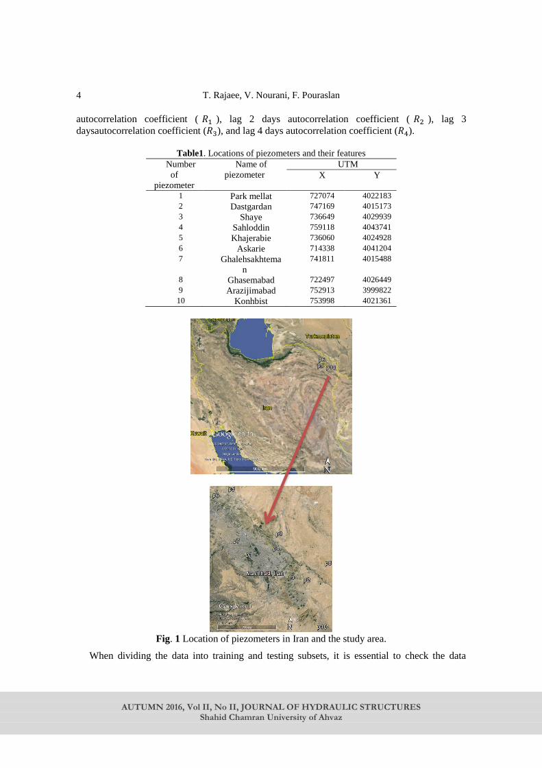
names and locations of these piezometers and Fig. 2 shows the time series of this data.
2.1. Statistical analysis The statistical analysis for training and testing sets is given in Table 2 to 5, which contains
the minimum, maximum, standard deviation (𝑆𝑑), mean, skewness coefficient (𝐶𝑠), lag 1 day
T. Rajaee, V. Nourani, F. Pouraslan
AUTUMN 2016, Vol II, No II, JOURNAL OF HYDRAULIC STRUCTURES
Shahid Chamran University of Ahvaz
4
autocorrelation coefficient ( 𝑅1 ), lag 2 days autocorrelation coefficient ( 𝑅2 ), lag 3
daysautocorrelation coefficient (𝑅3), and lag 4 days autocorrelation coefficient (𝑅4).
Table1. Locations of piezometers and their features
Number
of
piezometer
Name of
piezometer
UTM
X Y
1 Park mellat 727074 4022183
2 Dastgardan 747169 4015173
3 Shaye 736649 4029939
4 Sahloddin 759118 4043741
5 Khajerabie 736060 4024928
6 Askarie 714338 4041204
7 Ghalehsakhtema
n
741811 4015488
8 Ghasemabad 722497 4026449
9 Arazijimabad 752913 3999822
10 Konhbist 753998 4021361
Fig. 1 Location of piezometers in Iran and the study area.
When dividing the data into training and testing subsets, it is essential to check the data
Groundwater Level Forecasting Using Wavelet and Kriging
AUTUMN 2016, Vol II, No II, JOURNAL OF HYDRAULIC STRUCTURES
Shahid Chamran University of Ahvaz
5
which present the same statistical population (Masters, 1993). In general, Table 2 to 5 illustrates
relatively similar statistical characteristics between the training and testing sets.
980
982
984
986
988
1 12 23 34 45 56 67 78 89 100
GW
L (
m)
time (month)
Piezometer number 1
Observed groundwater…
872
874
876
878
1
12
23
34
45
56
67
78
89
10
0
GW
L (
m)
time (month)
Piezometer number 2 Observed…
874
879
884
889
1 12 23 34 45 56 67 78 89 100
GW
L (
m)
time (month)
Piezometer number 3 Observed groundwater…
992
994
996
998
1 12 23 34 45 56 67 78 89 100
GW
L (
m)
time (month)
Piezometer number 4 Observed groundwater…
942
944
946
948
950
1
12
23
34
45
56
67
78
89
10
0
GW
L (
m)
time (month)
Piezometer number 5
Observed groundwater…
986
991
996
1001
1 12 23 34 45 56 67 78 89 100
GW
L (
m)
time (month)
Piezometer number 6
Observed groundwater…

T. Rajaee, V. Nourani, F. Pouraslan
AUTUMN 2016, Vol II, No II, JOURNAL OF HYDRAULIC STRUCTURES
Shahid Chamran University of Ahvaz
6
Fig. 2 Monthly changes in GWL in the period time for each piezometer
Table 2. Statistics analysis for training, testing and all data sets. Statistical
parameters
Piezometer
(1)
Piezometer
(2)
Piezometer
(3)
All data
Training set Testing set
All data
Training set Testing set
All data
Training set Testing set
Number of
data
102 90 12 102 90 12 102 90 12
Mean 984.05 983.95 984.76 875.37 875.38 875.3 881.5 881.81 879.94
Max 986.58 985.61 985.61 878.22 878.22 875.71 888.58 888.58 882.87
Min 982.22 982.22 983.48 872.51 874.18 872.51 876.52 876.97 876.52
𝑆𝑑 1.13 1.14 0.76 0.54 1.14 0.54 2.52 2.5 2.05
Cs 0.3 0.47 -0.65 -1.26 -0.41 -1.26 0.39 0.4 -0.26
𝑅1 0.89 0.9 0.72 0.9 0.89 0.9 0.84 0.84 0.86
𝑅2 0.78 0.78 0.29 0.81 0.78 0.81 0.57 0.56 0.51
𝑅3 0.64 0.63 -0.26 0.63 0.65 0.63 0.26 0.24 0.12
𝑅4 0.51 0.48 -0.63 0.5 0.51 0.5 -0.05 -0.08 -0.22
Table 3. Statistics analysis for training, testing and all data sets.
Statistical
parameters
Piezometer
(4)
Piezometer
(5)
Piezometer
(6)
All
data
Training set Testing
set
All
data
Training set Testing
set
All
data
Training set Testing
set
Number of
data
102 90 12 102 90 12 102 90 12
Mean 995.24 995.44 993.79 944.62 944.36 946.54 993.51 994 989.86
880
885
890
1
12
23
34
45
56
67
78
89
10
0
GW
L (
m)
time (month)
Piezometer number 7 Observed ground…
976978980982984986988990992994996998
1 12 23 34 45 56 67 78 89 100
GW
L (
m)
time (month)
Piezometer number 8 Observed groundwater…
903
908
913
1 12 23 34 45 56 67 78 89 100
GW
L (
m)
time (month)
Piezometer number 9 Observed groundwater…
859
860
861
862
1 12 23 34 45 56 67 78 89 100
GW
L (
m)
time (month)
Piezometer number 10 Observed groundwater…
Groundwater Level Forecasting Using Wavelet and Kriging
AUTUMN 2016, Vol II, No II, JOURNAL OF HYDRAULIC STRUCTURES
Shahid Chamran University of Ahvaz
7
Max 998.36 998.36 994.51 949.53 949.53 947.55 1000.92 1000.92 991.61 Min 992.83 992.83 993.04 942.51 942.51 945.22 987.51 987.51 988.64
𝑆𝑑 1.39 1.36 0.44 1.85 1.8 0.72 3.6 3.54 0.95
Cs 0.27 0.11 -0.22 1.14 1.6 -0.27 0.3 0.12 -0.3
𝑅1 0.96 0.96 0.96 0.93 0.92 0.91 0.97 0.98 0.92
𝑅2 0.9 0.89 0.83 0.85 0.83 0.74 0.94 0.94 0.74
𝑅3 0.82 0.8 -0.61 0.76 0.72 0.52 0.91 0.9 0.57
𝑅4 0.75 0.72 -0.27 0.67 0.62 0.28 0.87 0.86 -0.42
Table 4. Statistics analysis for training, testing and all data sets.
Statistical
parameters
Piezomet
er (7)
Piezomet
er (8)
Piezomet
er (9)
All data Training
set
Testing
set
All data Training
set
Testing set All data Training
set
Testing
set
Number of
data
102 90 12 102 90 12 102 90 12
Mean 885.04 884.7 887.65 985.1 984.75 987.71 993.51 994 989.86
Max 893.25 893.25 889.31 1039.31 997.06 1039.31 1000.92 1000.92 991.61
Min 881.27 881.27 884.25 978.39 978.39 982.46 987.51 987.51 988.64
𝑆𝑑 3.07 3.04 1.83 7.45 5.42 16.26 3.6 3.54 0.95
Cs 1.27 1.65 -0.89 4.02 0.76 3 0.3 0.12 -0.3
𝑅1 0.92 0.93 0.75 0.4 0.95 0.98 0.97 0.98 0.92
𝑅2 0.8 0.81 0.33 0.36 0.9 0.96 0.94 0.94 0.74
𝑅3 0.69 0.67 -0.17 0.51 0.84 0.93 0.91 0.9 0.57
𝑅4 0.57 0.54 -0.64 0.49 0.79 0.91 0.87 0.86 -0.42
Table 5. Statistics analysis for training, testing and all data sets.
Statistical
parameters
Piezometer
(10)
All
data
Training
set
Testing
set
Number of
data
102 90 12
Mean 860.58 860.58 860.55
Max 861.89 861.89 861..36
Min 859.54 859.54 859.73
𝑆𝑑 0.61 0.62 0.54
Cs 0.29 0.32 -0.3
𝑅1 0.86 0.88 0.96
𝑅2 0.72 0.76 0.92
𝑅3 0.61 0.7 0.83
𝑅4 0.59 0.7 0.75
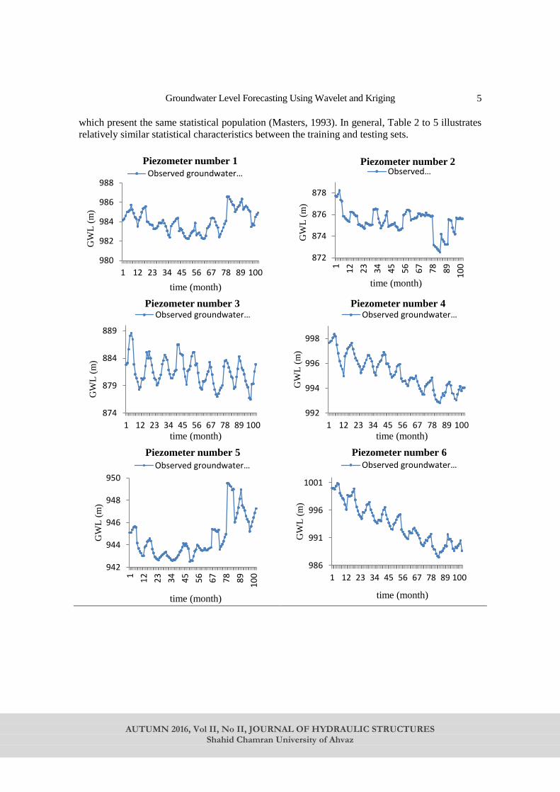
According to Table 2 to 5, the results show that piezometer (8) has a higher standard
deviation compared with other piezometers and the difference between testing and training data
is more than those of other piezometers.
Almost for all piezometers except piezometer (8), skewness coefficients were low for both
training and testing sets. This is appropriate for modelling, because a high skewness coefficient
has a considerable negative effect on the ANN performance (Altun et al., 2007).
Piezometer (8) had the most difference between all data, training and testing data.
There are more differences in lag 3 months and 4 months autocorrelation coefficient for
piezometers (1), (4), (6), (7) and (9) between all data, training and testing data.
Overall, Table 2 to 5 shows a relative similarity between testing and training data and it is
suitable for ANN performance. The results of our study showed that, these slight differences did
not have a serious impact.
In this study, the data were pre-processed and for this purpose the following simple linear
T. Rajaee, V. Nourani, F. Pouraslan
AUTUMN 2016, Vol II, No II, JOURNAL OF HYDRAULIC STRUCTURES
Shahid Chamran University of Ahvaz
8
mapping of the variables were used. For the x variable, the scaled value x_n was computed as
follows:
𝑥𝑛 =(𝑥−𝑥𝑚𝑖𝑛)
(𝑥𝑚𝑎𝑥−𝑥𝑚𝑖𝑛) (1)
3. Methods
3.1. Artificial neural network analysis The first fundamental concepts related to neural computing were developed by McCulloch
and Pitts (1943). Artificial neural networks were inspired by biological findings related to the
behaviour of the brain as a network of units called neurons (Rumelhart et al., 1986). A common
three-layered feed-forward neural network is comprised of multiple elements, called nodes, and
connection pathways that link them (Haykin, 1999). These networks contain an input layer, a
hidden layer and an output layer. The input layer consists of nodes representing different input
variables; the hidden layer consists of many hidden nodes; and the output layer consists of
output variables. The net input to unit i is:
𝑦𝑖 = ∑ 𝑤𝑖𝑗𝑥𝑖 + 𝜃𝑖𝑝𝑗=1 (2)
Where 𝑤𝑗𝑖 = (𝑤1, 𝑤2, … 𝑤𝑝𝑖) is the weight vector of unit 𝑖 and 𝑝 is the number of neurons in
the above layer of unit 𝑖, 𝑥𝑖 is the output from unit 𝑗 and 𝜃𝑖 is the bias of unit 𝑖. This weighted
sum 𝑦𝑖, which is called the incoming signal of unit 𝑖, is then passed through a transfer function.
A recommended literature for the ANN approach could be Masters (1993).
3.2. Wavelet analysis Wavelet is a small wave energy of which is restricted to a short period of time and it is an
efficient method for signals that are non-stationary, and have short-lived transient components,
features at different scales, or singularities (Hsu & Li., 2010). Wavelet transform is a modern
tool and a signal processing technique. It has shown a higher performance compared to the
Fourier transform. The Wavelet transform performs the decomposition of a signal into a group
of functions (Cohen & Kovacevic, 1996):
𝜓𝑗,𝑘(𝑥) = 2𝑗
2⁄ 𝜓𝑗,𝑘(2𝑗𝑥 − 𝑘) (3)
Where 𝜓𝑗,𝑘(𝑥) is produced from a mother wavelet 𝜓(𝑥) which is dilated by 𝑗 and translated
by 𝑘. The mother wavelet has to satisfy the condition.
∫ ψ(x)dx = 0 (4)
The discrete wavelet function of a signal f(x) can be calculated as follows:
𝑐𝑗,𝑘 = ∫ 𝑓(𝑥)𝜓𝑗,𝑘∗∞
−∞(𝑥)𝑑𝑥 (5)
f(x) = ∑ cj,kψj,k(x)j,k (6)
Where, 𝑐𝑗,𝑘is the approximate coefficient of a signal. The mother wavelet is formulated from the
scaling function 𝜑(𝑥) as:
φ(𝑥) = √2 ∑ ℎ0(𝑛)𝜑(2𝑥 − 𝑛) (7)
ψ(x) = √2 ∑ h1(n)φ(2x − n) (8)
Groundwater Level Forecasting Using Wavelet and Kriging
AUTUMN 2016, Vol II, No II, JOURNAL OF HYDRAULIC STRUCTURES
Shahid Chamran University of Ahvaz
9
Where ℎ1(𝑛) = (−1)𝑛ℎ0(1 − 𝑛) . Different sets of coefficients ℎ0(𝑛) canbe found
corresponding to wavelet bases with various characteristics.In the DWT, coefficients ℎ0(𝑛)play
a critical role (Gupta & Gupta., 2007).
3.3. Geostatistics analysis Geostatistics was originally developed for estimation of ore reserves in mining (Einax & Soldt.,
1999). The main tool in geostatistics is the variogram, which expresses the spatial dependence
between neighbouring observations. Prior to the geostatistical estimation, we require a model
that enables us to compute a variogram value for any possible sampling interval. The most
commonly used models are spherical, exponential, Gaussian, and pure nugget effect (Isaaks &
Srivastava, 1989). The variogram quantifies the relationship between the variance and the
distance between sampling pairs by the following equation (Isaaks & Srivastava, 1989,
Kitanidis, 1997):
γ(h) =1
2N(h)∑ (Z(xi + h) − Z(xi))2N(h)
i=1 (9)
Where 𝑁(ℎ) is the number of data pairs within a given class of distances and directions. And
𝑍(𝑥𝑖) and 𝑍(𝑥𝑖 + ℎ) are observations of the variable Z at spatial locations 𝑥𝑖 and 𝑥𝑖 + ℎ.
One of the geostatistics methods is the kriging technique. Only a brief description of the
Kriging method is employed in this research.
3.3.1. Kriging
Kriging technique is an exact interpolation estimator 𝑍(𝑥0)used to find the best linear
unbiased estimator of a second estimator of a second order stationary. The general form of
kriging equation is:
Z(x0) = ∑ λiZ(xi)ni=1 (10)
Where Z(𝑥0) is Kriging estimate at location𝑥0; Z(𝑥𝑖) is sampledvalue at 𝑥𝑖;𝜆𝑖 is
weighting factor for Z(𝑥𝑖); and 𝑖 = 1, . . . , 𝑛 inwhich n denotes to the numbers of samples.
4. Model application The method proposed in this study consists of three distinct stages to achieve the best
result. For temporal GWL estimating at the first stage, an ANN was trained and tested for
each piezometer for time series modelling of the water level. The model predicted GWL of
the piezometers for the next month.
In the next stage, the WANN model was used. In this method, the decomposed GWL
time series are entered into the ANN method for prediction of GWL one month ahead. At
the end of these two-stages, the best result of these two methods were selected. And in the
last stage, the spatial (GWL) was forecasted in the study area with the kriging technique.
4.1 model evaluation Some performance evaluation criteria such as correlation coefficient are unsuitable for
model evaluation (Legates & McCabe; 1999). One of the suitable criteria proposed by such
researches is that a perfect evaluation of a model performance should include at least one
‘goodness-of-fit’ or relative error measure (e.g. coefficient of determination ( R2 )); this
criteria can be used to compare the relative performances of the models developed by
different methods. It is estimated as (Nash & Sutcliffe (1970)).𝑅2 and at least one absolute
error measure (e.g. root mean square error (RMSE)) and (e.g. mean absolute error (MAE))
T. Rajaee, V. Nourani, F. Pouraslan
AUTUMN 2016, Vol II, No II, JOURNAL OF HYDRAULIC STRUCTURES
Shahid Chamran University of Ahvaz
10
were used to assess the effectiveness of each model. The best fit between the observed and
calculated values would have R2=1, RMSE=0 and MAE=0.
R2 = 1 −∑ (GWLi(measured)−GWLi(predicted))
2ni=1
∑ (GWLi(measured)−GWLi(mean))2n
i=1
(11)
MAE =∑ |GWLi(measued)−GWLi(predicted)|n
i=1
n (12)
RMSE = √∑ (GWLi(measured)−GWLi(predicted))2n
i=1
n (13)
Where n is the number of the data points.
4.2. Application of ANN In this study, a three-layered feed forward neural network (FFNN) with a back
propagation (BP) algorithm (Masters., 1993; Haykin, 1999) was used. This algorithm is a
gradient descent procedure and consists of one input layer, one hidden layer, and one output
layer. The BP algorithm was employed to minimize a least-square objective function (error
function). The Levenberg–Marquardt (LM) algorithm (Haykin., 1999) was used to train
ANN models. The LM method is a modification of the classic Newton algorithm for finding
an optimum solution to a minimization problem (Nouraniet al., 2011). The Sigmoid and
Tansig (Schmitz et al., 2006) functions were used as activation functions in the hidden and
output layer nodes to make the ANN model more effective. The Sigmoid function is
differentiable, continuous, and monotonically increasing in its domain and it is the most
frequently employed function. The numbers of the hidden layer nodes and training epochs
(the training iteration number) are determined by trial and error in the test scenarios. Firstly,
the training phase is completed; then, the testing phase begins using the optimum values
found for the number of neurons in each input layer and hidden layer. The artificial neural network model used in this study was the Nonlinear Auto Regressive
(NAR) model. NAR neural networks can be trained to predict a time series from the past
values of that series.
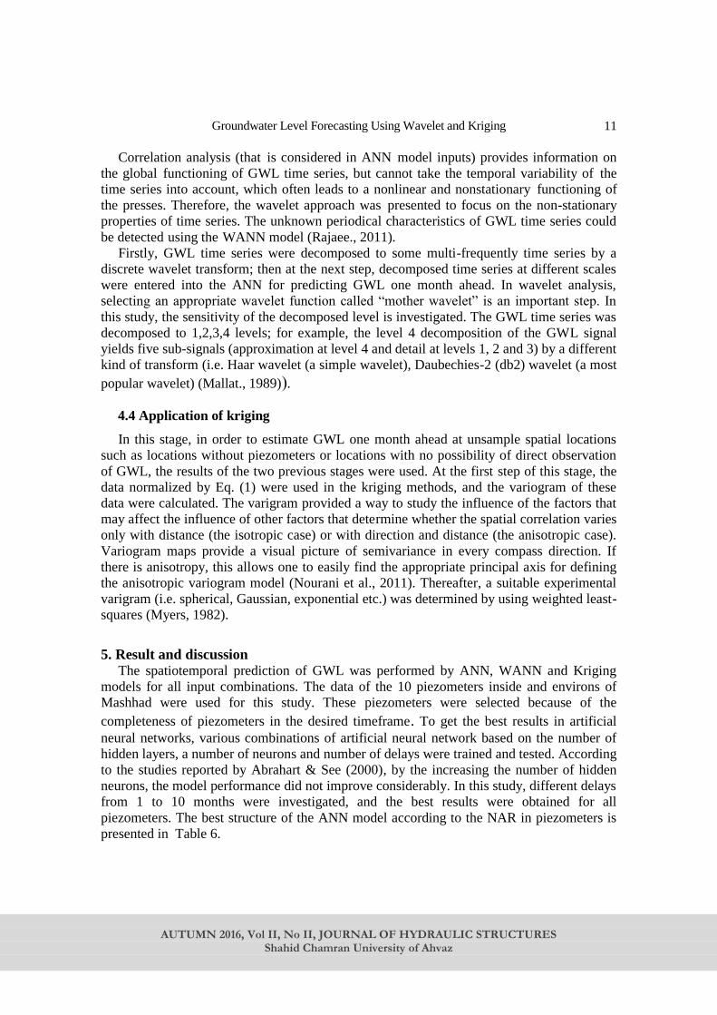
4.3. Application of WANN In the WANN model, the decomposed GWL time series was linked to the ANN method
for the prediction of GWL one month ahead. The proposed WANN model for the prediction
of GWL is shown in Fig. 3.
Fig 3. Structure of the proposed WANN combination model
Groundwater Level Forecasting Using Wavelet and Kriging
AUTUMN 2016, Vol II, No II, JOURNAL OF HYDRAULIC STRUCTURES
Shahid Chamran University of Ahvaz
11
Correlation analysis (that is considered in ANN model inputs) provides information on
the global functioning of GWL time series, but cannot take the temporal variability of the
time series into account, which often leads to a nonlinear and nonstationary functioning of
the presses. Therefore, the wavelet approach was presented to focus on the non-stationary
properties of time series. The unknown periodical characteristics of GWL time series could
be detected using the WANN model (Rajaee., 2011).
Firstly, GWL time series were decomposed to some multi-frequently time series by a
discrete wavelet transform; then at the next step, decomposed time series at different scales
were entered into the ANN for predicting GWL one month ahead. In wavelet analysis,
selecting an appropriate wavelet function called “mother wavelet” is an important step. In
this study, the sensitivity of the decomposed level is investigated. The GWL time series was
decomposed to 1,2,3,4 levels; for example, the level 4 decomposition of the GWL signal
yields five sub-signals (approximation at level 4 and detail at levels 1, 2 and 3) by a different
kind of transform (i.e. Haar wavelet (a simple wavelet), Daubechies-2 (db2) wavelet (a most
popular wavelet) (Mallat., 1989)(.
4.4 Application of kriging
In this stage, in order to estimate GWL one month ahead at unsample spatial locations
such as locations without piezometers or locations with no possibility of direct observation
of GWL, the results of the two previous stages were used. At the first step of this stage, the
data normalized by Eq. (1) were used in the kriging methods, and the variogram of these
data were calculated. The varigram provided a way to study the influence of the factors that
may affect the influence of other factors that determine whether the spatial correlation varies
only with distance (the isotropic case) or with direction and distance (the anisotropic case).
Variogram maps provide a visual picture of semivariance in every compass direction. If
there is anisotropy, this allows one to easily find the appropriate principal axis for defining
the anisotropic variogram model (Nourani et al., 2011). Thereafter, a suitable experimental
varigram (i.e. spherical, Gaussian, exponential etc.) was determined by using weighted least-
squares (Myers, 1982).
5. Result and discussion The spatiotemporal prediction of GWL was performed by ANN, WANN and Kriging
models for all input combinations. The data of the 10 piezometers inside and environs of
Mashhad were used for this study. These piezometers were selected because of the
completeness of piezometers in the desired timeframe. To get the best results in artificial
neural networks, various combinations of artificial neural network based on the number of
hidden layers, a number of neurons and number of delays were trained and tested. According
to the studies reported by Abrahart & See (2000), by the increasing the number of hidden
neurons, the model performance did not improve considerably. In this study, different delays
from 1 to 10 months were investigated, and the best results were obtained for all
piezometers. The best structure of the ANN model according to the NAR in piezometers is
presented in Table 6.
T. Rajaee, V. Nourani, F. Pouraslan
AUTUMN 2016, Vol II, No II, JOURNAL OF HYDRAULIC STRUCTURES
Shahid Chamran University of Ahvaz
12
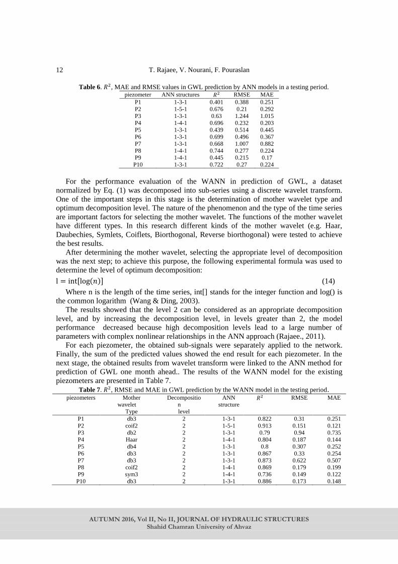
Table 6. 𝑅2, MAE and RMSE values in GWL prediction by ANN models in a testing period. piezometer ANN structures 𝑅2 RMSE MAE
P1 1-3-1 0.401 0.388 0.251
P2 1-5-1 0.676 0.21 0.292
P3 1-3-1 0.63 1.244 1.015
P4 1-4-1 0.696 0.232 0.203
P5 1-3-1 0.439 0.514 0.445
P6 1-3-1 0.699 0.496 0.367
P7 1-3-1 0.668 1.007 0.882
P8 1-4-1 0.744 0.277 0.224
P9 1-4-1 0.445 0.215 0.17
P10 1-3-1 0.722 0.27 0.224
For the performance evaluation of the WANN in prediction of GWL, a dataset
normalized by Eq. (1) was decomposed into sub-series using a discrete wavelet transform.
One of the important steps in this stage is the determination of mother wavelet type and
optimum decomposition level. The nature of the phenomenon and the type of the time series
are important factors for selecting the mother wavelet. The functions of the mother wavelet
have different types. In this research different kinds of the mother wavelet (e.g. Haar,
Daubechies, Symlets, Coiflets, Biorthogonal, Reverse biorthogonal) were tested to achieve
the best results.
After determining the mother wavelet, selecting the appropriate level of decomposition
was the next step; to achieve this purpose, the following experimental formula was used to
determine the level of optimum decomposition:
l = int[log(𝑛)] (14)
Where n is the length of the time series, int[] stands for the integer function and log() is
the common logarithm (Wang & Ding, 2003). The results showed that the level 2 can be considered as an appropriate decomposition
level, and by increasing the decomposition level, in levels greater than 2, the model
performance decreased because high decomposition levels lead to a large number of
parameters with complex nonlinear relationships in the ANN approach (Rajaee., 2011).
For each piezometer, the obtained sub-signals were separately applied to the network.
Finally, the sum of the predicted values showed the end result for each piezometer. In the
next stage, the obtained results from wavelet transform were linked to the ANN method for
prediction of GWL one month ahead.. The results of the WANN model for the existing
piezometers are presented in Table 7.
Table 7. 𝑅2, RMSE and MAE in GWL prediction by the WANN model in the testing period. piezometers Mother
wavelet
Type
Decompositio
n
level
ANN
structure 𝑅2 RMSE MAE
P1 db3 2 1-3-1 0.822 0.31 0.251
P2 coif2 2 1-5-1 0.913 0.151 0.121
P3 db2 2 1-3-1 0.79 0.94 0.735
P4 Haar 2 1-4-1 0.804 0.187 0.144
P5 db4 2 1-3-1 0.8 0.307 0.252
P6 db3 2 1-3-1 0.867 0.33 0.254
P7 db3 2 1-3-1 0.873 0.622 0.507
P8 coif2 2 1-4-1 0.869 0.179 0.199
P9 sym3 2 1-4-1 0.736 0.149 0.122
P10 db3 2 1-3-1 0.886 0.173 0.148
Groundwater Level Forecasting Using Wavelet and Kriging
AUTUMN 2016, Vol II, No II, JOURNAL OF HYDRAULIC STRUCTURES
Shahid Chamran University of Ahvaz
13
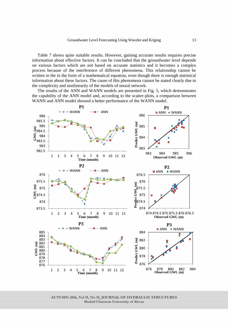
Table 7 shows quite suitable results. However, gaining accurate results requires precise
information about effective factors. It can be concluded that the groundwater level depends
on various factors which are not based on accurate statistics and it becomes a complex
process because of the interference of different phenomena. This relationship cannot be
written in the in the form of a mathematical equation, even though there is enough statistical
information about these factors. The cause of this phenomena cannot be stated clearly due to
the complexity and nonlinearity of the models of neural network.
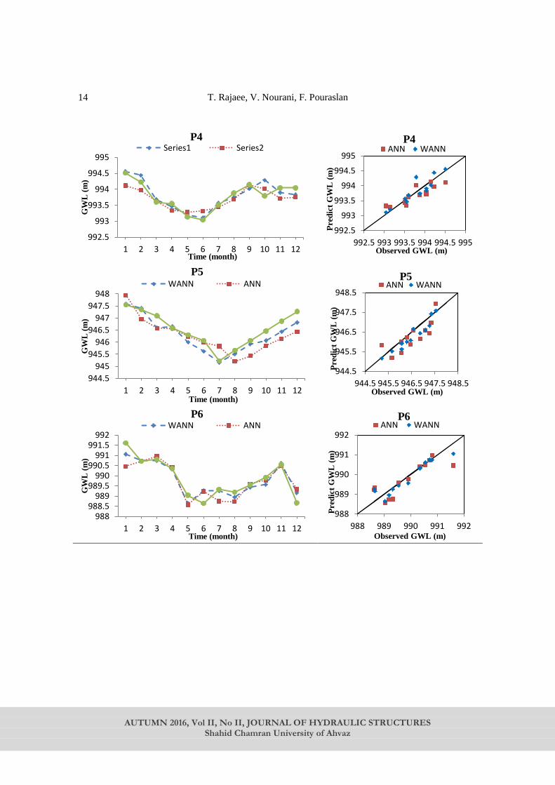
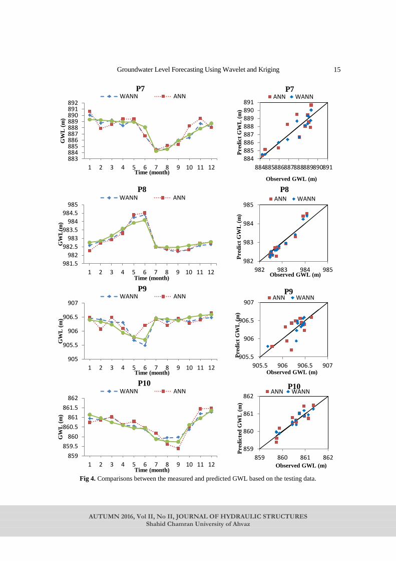
The results of the ANN and WANN models are presented in Fig. 5, which demonstrates
the capability of the ANN model and, according to the scatter-plots, a comparison between
WANN and ANN model showed a better performance of the WANN model.
982.5
983
983.5
984
984.5
985
985.5
986
1 2 3 4 5 6 7 8 9 10 11 12
GW
L (
m)
Time (month)
P1 WANN ANN
983
984
985
986
983 984 985 986
Pre
dic
t G
WL
(m
)
Observed GWL (m)
P1 ANN WANN
873.5
874
874.5
875
875.5
876
1 2 3 4 5 6 7 8 9 10 11 12
GW
L (
m)
Time (month)
P2 WANN ANN
874
874.5
875
875.5
876
876.5
874 874.5 875 875.5 876 876.5
Pre
dic
t G
WL
(m
)
Observed GWL (m)
P2 ANN WANN
876877878879880881882883884885
1 2 3 4 5 6 7 8 9 10 11 12
GW
L (
m)
Time (month)
P3 WANN ANN
876
878
880
882
884
876 878 880 882 884
Pre
dic
t G
WL
(m
)
Observed GWL (m)
P3 ANN WANN
T. Rajaee, V. Nourani, F. Pouraslan
AUTUMN 2016, Vol II, No II, JOURNAL OF HYDRAULIC STRUCTURES
Shahid Chamran University of Ahvaz
14
992.5
993
993.5
994
994.5
995
1 2 3 4 5 6 7 8 9 10 11 12
GW
L (
m)
Time (month)
P4 Series1 Series2
992.5
993
993.5
994
994.5
995
992.5 993 993.5 994 994.5 995
Pre
dic
t G
WL
(m
)
Observed GWL (m)
P4 ANN WANN
944.5
945
945.5
946
946.5
947
947.5
948
1 2 3 4 5 6 7 8 9 10 11 12
GW
L (
m)
Time (month)
P5 WANN ANN
944.5
945.5
946.5
947.5
948.5
944.5 945.5 946.5 947.5 948.5
Pre
dic
t G
WL
(m
)
Observed GWL (m)
P5 ANN WANN
988988.5
989989.5
990990.5
991991.5
992
1 2 3 4 5 6 7 8 9 10 11 12
GW
L (
m)
Time (month)
P6 WANN ANN
988
989
990
991
992
988 989 990 991 992
Pre
dic
t G
WL
(m
)
Observed GWL (m)
P6 ANN WANN
Groundwater Level Forecasting Using Wavelet and Kriging
AUTUMN 2016, Vol II, No II, JOURNAL OF HYDRAULIC STRUCTURES
Shahid Chamran University of Ahvaz
15
Fig 4. Comparisons between the measured and predicted GWL based on the testing data.
883884885886887888889890891892
1 2 3 4 5 6 7 8 9 10 11 12
GW
L (
m)
Time (month)
P7 WANN ANN
884885886887888889890891
884885886887888889890891
Pre
dic
t G
WL
(m
)
Observed GWL (m)
P7 ANN WANN
981.5
982
982.5
983
983.5
984
984.5
985
1 2 3 4 5 6 7 8 9 10 11 12
GW
L(m
)
Time (month)
P8 WANN ANN
982
983
984
985
982 983 984 985
Pre
dic
t G
WL
(m
)
Observed GWL (m)
P8 ANN WANN
905
905.5
906
906.5
907
1 2 3 4 5 6 7 8 9 10 11 12
GW
L (
m)
Time (month)
P9 WANN ANN
905.5
906
906.5
907
905.5 906 906.5 907
Pre
dic
t G
WL
(m
)
Observed GWL (m)
P9 ANN WANN
859
859.5
860
860.5
861
861.5
862
1 2 3 4 5 6 7 8 9 10 11 12
GW
L (
m)
Time (month)
P10 WANN ANN
859
860
861
862
859 860 861 862
Pre
dic
ted
GW
L (
m)
Observed GWL (m)
P10 ANN WANN

T. Rajaee, V. Nourani, F. Pouraslan
AUTUMN 2016, Vol II, No II, JOURNAL OF HYDRAULIC STRUCTURES
Shahid Chamran University of Ahvaz
16
Anticipated maximum and minimum points of GWL are important in the design of hydraulic
structures, and it can be a good feature of the hydrological model. Table 8 compares the
performance of these two models. According to this table, in this part, the WANN model has
better results, too.
Table 8. Performance of models to forecast the peak of groundwater level.
Number of piezometer Observed GWL
Abrupt changes
ANN WANN
P1 0.13 -0.05 0.04
-1.85 -0.08 -0.56
P2 1.53 1.85 0.52
0 -0.06 -0.04
P3 0.06 1.3 1.12
2.75 2.56 3
P4 -0.63 -0.35 -0.75
0 0.04 -0.07
P5 0.23 0.24 0.37
0.85 0.15 0.47
P6 0.1 0.23 0
-1.89 -1.16 -1.46
P7 0 -0.05 0.98
-3.83 -2.28 -2.13
P8 -1.58 -2.06 -1.9
-0.01 -0.13 -0.13
P9 0.76 0.22 0.99
-0.02 -0.22 -0.14
P10 0 -0.33 -0.17
0.88 1.15 0.4
The sum of the
absolute values of the
predicted values
17.1 14.51 15.24
Percent error %15 %11
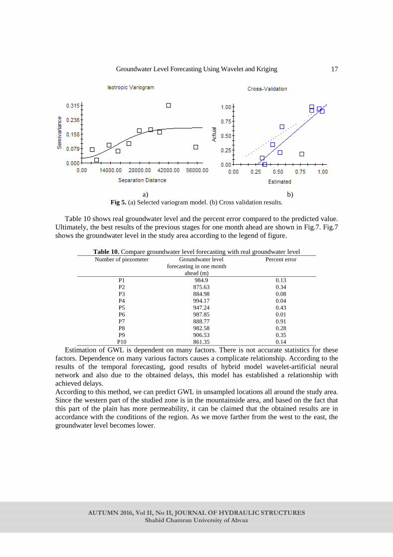
According to the best results obtained in the previous steps, the best variogram of the data
was plotted using the values of the GWLs at different piezometers. An appropriate variogram
model was plotted by fitting such variogram models. The geostatistical model, which leads to the
least RMSE was selected by comparing the observed GWL values with the values estimated by
variogram models (Nourani et al, 2011).
The results of the best-fitted model are presented in Table 9; this model is selected based on
the least values of RMSE and RSS among other models.
Table 9. Rresults of different variogram models.
Model RMSE
Spherical 0.260
*Gaussian 0.253
Exponential 0.268
Linear 1.005
According to Table 5, the Gaussian model was a suitable one. This model is shown in Fig.
5.a. Fig. 5.b shows the results of cross-validation method as a scatter plot, which determines the
liability of the proposed geostatistical modelling according to the normalized data.
Groundwater Level Forecasting Using Wavelet and Kriging
AUTUMN 2016, Vol II, No II, JOURNAL OF HYDRAULIC STRUCTURES
Shahid Chamran University of Ahvaz
17
a) b)
Fig 5. (a) Selected variogram model. (b) Cross validation results.
Table 10 shows real groundwater level and the percent error compared to the predicted value.
Ultimately, the best results of the previous stages for one month ahead are shown in Fig.7. Fig.7
shows the groundwater level in the study area according to the legend of figure.
Table 10. Compare groundwater level forecasting with real groundwater level Number of piezometer Groundwater level
forecasting in one month
ahead (m)
Percent error
P1 984.9 0.13
P2 875.63 0.34
P3 884.98 0.08
P4 994.17 0.04
P5 947.24 0.43
P6 987.85 0.01
P7 888.77 0.91
P8 982.58 0.28
P9 906.53 0.35
P10 861.35 0.14
Estimation of GWL is dependent on many factors. There is not accurate statistics for these
factors. Dependence on many various factors causes a complicate relationship. According to the
results of the temporal forecasting, good results of hybrid model wavelet-artificial neural
network and also due to the obtained delays, this model has established a relationship with
achieved delays. According to this method, we can predict GWL in unsampled locations all around the study area.
Since the western part of the studied zone is in the mountainside area, and based on the fact that
this part of the plain has more permeability, it can be claimed that the obtained results are in
accordance with the conditions of the region. As we move farther from the west to the east, the
groundwater level becomes lower.

T. Rajaee, V. Nourani, F. Pouraslan
AUTUMN 2016, Vol II, No II, JOURNAL OF HYDRAULIC STRUCTURES
Shahid Chamran University of Ahvaz
18
Fig 7. groundwater level forecasting in study area
6. Summary and conclusion In the current study, an attempt was made to investigate the capability of the proposed hybrid
empirical models for spatiotemporal GWL forecasting. This model was applied for Mashhad
City and its environs in the Northeast Iran at Khorasan Razavi Province. Firstly, for temporal
forecasting stage by comparison of the prediction accuracies of ANN and WANN models
indicated that the proposed WANN model with coefficient of determination and root mean
square error and mean absolute error, 0.836 and 0.335 and 0.273 respectively, showed better
results. GWL signals were decomposed into sub-signals with different scales, and this
decomposed GWL time series was used as input data to the ANN models for prediction of GWL
one month ahead. The results showed that the right choice of the mother wavelet and optimum
decomposed level lead to a more precise prediction, and increasing the decomposition level, lead
to low efficiency.
Then, in the spatial estimation stage, the kriging method was applied to the outputs from the
WANN models to estimate GWL in the environs of Mashhad City one month ahead, especially
in unsampled locations. A Gaussian model with 0.253 in RMSE had the best result among other
variograms.
In order to extend the presented model, adding some forecasting sub-models for modelling
the input hydrological parameters of the model such as temperature or precipitation intensity or
evapotranspiration or using other interpolation methods in geostatistics like Cokriging or Spline
or Inverse Distance Weighting (IDW) is recommended for future researches.
References
1. Rajaee, T., 2011. Wavelet and ANN combination model for prediction of daily suspended
sediment load in rivers. Science of the Total Environment, 409: 2917–2928.
2. Rajaee, T., Broumand, A., 2015. Forecasting of chlorophyll-a concentrations in South San
Francisco Bay using five different models. Applied Ocean Research, 53: 208–217.
Groundwater Level Forecasting Using Wavelet and Kriging
AUTUMN 2016, Vol II, No II, JOURNAL OF HYDRAULIC STRUCTURES
Shahid Chamran University of Ahvaz
19
3. Ravansalar, M., Rajaee, T., 2015. Evaluation of Wavelet Performance via an ANN-Based
Electrical Conductivity Prediction model. Environmental Monitoring and Assessment
187:366. DOI 10.1007/s10661-015-4590-7.
4. Yang, Z.P., Lu, W.X., Long, Y.Q., Li, P., 2009. Application and comparison of two
prediction models for groundwater levels: A case study in Western Jilin Province, China.
Journal of Arid Environments, 73: 487–492.
5. Shiri, J., Kisi, O., 2011. Comparison of genetic programming with neuro-fuzzy systems for
predicting short-term water table depth fluctuations. Computers and Geosciences, 37: 1692-
1701.
6. Yoon, H., Jun, S., Hyun, Y., Bae, G., Lee, K., 2011. A comparative study of artificial neural
networks and support vector machines for predicting groundwater levels in a coastal
aquifer. Journal of Hydrology, 396: 128–138.
7. Mohammadi, K., 2008. Groundwater table estimation using MODFLOW and artificial
neural networks. Water Science and Technology Library 68, no. 2: 127-138.
8. Nourani, V., Goli Ejlali, R, and Alami, M.T., 2011. Spatiotemporal Groundwater Level
Forecasting in Coastal Aquifers by Hybrid Artificial Neural Network-Geostatistics Model:
A Case Study. Environmental Engineering Science, 28(3): 217-228.
9. Nakhaei, M., Saberi Nasr, A., 2012. A combined Wavelet- Artificial Neural Network model
and its application to the prediction of groundwater level fluctuations. Geopersia, 2 (2): 77-
91.
10. Zhou, H.C., Peng, Y., Liang, G.H., 2008. The research of monthly discharge predictor-
corrector model based on wavelet decomposition. Water ResourcesManagement, 22: 217–
227.
11. Kisi, O., 2010. Wavelet regression model for short-term streamflow forecasting. Journal of
Hydrology 389: 344–353.
12. Gemitzi, A., Stefanopoulos, K., 2011. Evaluation of the effects of climate and man
intervention on ground waters and their dependent ecosystems using time series analysis.
Journal of Hydrology 403: 130–140.
13. Wang, W., Jin, J., Li, Y, 2009. Prediction of inflow at three gorges dam in Yangtze river
with wavelet network model. Water Resources Management, 23: 2791–2083.
14. Sahoo GB, Ray C, Mehnert E, Keefer DA., 2006. Application of artificial neural networks
toassess pesticide contamination in shallow groundwater. Sci Total Environ, 367:234–51.
15. Rajaee T, Mirbagheri SA, Zounemat-Kermani M, Nourani V., 2009. Daily suspended
sedimentconcentration simulation using ANN and neuro-fuzzy models. Sci Total Environ,
407:4916–27.
16. Tsai CH, Chang LC, Chiang HC., 2009. Forecasting of ozone episode days by cost-
sensitiveneural network methods. Sci Total Environ. 407:2124–35.
17. Aziz, A.R.A., Wang, K.F.V., 1992. Neural networks approach the determination of aquifer
parameter. Groundwater, 30(2): 164-166.
18. Lallahem, S., Mania, J., Hani, A., Najjar, Y., 2005.On the use of neural networks to
evaluate groundwater levels in fractured media. Journal of Hydrology, 307: 92–111.
19. Daliakopoulos, I.N., Coulibaly, P., Tsanis, I.K., 2005. Groundwater level forecasting using
artificial neural networks. Journal of Hydrology, 309: 229–240.
20. Nourani, V., Mogaddam, A.A., and Nadiri, A., 2008. An ANNbasedmodel for
spatiotemporal groundwater level forecasting.Hydrological Processes. 22 (26): 5054-5066.
T. Rajaee, V. Nourani, F. Pouraslan
AUTUMN 2016, Vol II, No II, JOURNAL OF HYDRAULIC STRUCTURES
Shahid Chamran University of Ahvaz
20
21. Sahoo, S., Jha, MK., 2013. Groundwater-level prediction using multiple linear regression
and artificial neural network techniques: a comparative assessment. Hydrogeology Journal.
21(8): 1865-1887.
22. Maiti, S., Tiwari, R. K., 2014. A comparative study of artificial neural networks, Bayesian
neural networks and adaptive neuro-fuzzy inference system in groundwater level prediction.
Environmental Earth Sciences. 71(7): 3147-3160.
23. Pasquini A, Depetris P., 2007. Discharge trends and flow dynamics of South American
riversdraining the southern Atlantic seaboard: an overview. Journal of Hydrology, 333:385–
99.
24. Rajaee T., 2010. Wavelet and neuro-fuzzy conjunction approach for suspended sediment
prediction. Clean-Soli, Air, Water, 38(3):275–86.
25. Shoaib M, Shamseldin A.Y, Melville B.W., 2014. Comparative study of different wavelet
based neural network models for rainfall–runoff modeling. Journal of Hydrology, 515: 47–
58.
26. Nourani V, HosseiniBaghanam A, Adamowski J, Kisi O., 2014. Applications of hybrid
wavelet–Artificial Intelligence models in hydrology: A review. Journal of Hydrology, 514:
358–377.
27. Adamowski, J., Chan, H.F., 2011. A wavelet neural network conjunction model for
groundwater level forecasting. Journal of Hydrology, 407: 28–40.
28. Nourani, V., Alami, M., Aminfar, M., 2009.A combined neural-wavelet model for
prediction of Ligvanchai watershed precipitation. Engineering applications of Artificial
Intelligence, 22: 466–472.
29. Rouhani, Sh., & Meyers, D. E., 1990. Problems in space-time kriging of geohydrological
data. Mathematical Geology, 22:611–623.
30. Reghunath, R., Sreedhara Murthy, T. R., & Raghavan, B. R., 2005. Time series analysis to
monitor and assess water resources: A moving average approach. Environmental Monitoring and Assessment, 109:65–72.
31. Kumar, S., Sondhi, S. K., &Phogat, V., 2005. Network designfor groundwater level
monitoring in upper Bari Doab canaltract, Punjab, India. Irrigation and Drainage, 54:431–
442.
32. Abedian H, Mohammadi K, Rafiee R., 2013. Optimizing monitoring network of water table
by geostatistical methods. Journal of Geology and Mining Research, 5(9): 223-231.
33. Kholghi M, Hosseini S.M., 2009. Comparison of Groundwater Level Estimation Using
Neuro -fuzzy and Ordinary Kriging. Environmental Modelling & Assessment, 14(6): 729-
737.
34. Altun H, Bilgil A, Fidan BC., 2007. Treatment of multi-dimensional data to enhance neural network estimators in regression problems. Expert Syst Appl, 32(2):599–605.
35. McCulloch WS, Pitts WH., 1943. A logical calculus of the ideas immanent in neural nets.
Bull Math Biophys, 5:115–33.
36. Rumelhart, D.E., and McClelland, J.L., 1986. Parallel Distributed Processing: Explorations
in the Microstructure of Cognition, I andIi. Cambridge: MIT Press.
37. Haykin S., 1999. Neural network — a comprehensive foundation. Englewood Cliffs,
NJ:Prentice-Hall.
38. Masters T., 1993. Practical neural network recipes in C++. San Diego (CA): Academic
Press.

Groundwater Level Forecasting Using Wavelet and Kriging
AUTUMN 2016, Vol II, No II, JOURNAL OF HYDRAULIC STRUCTURES
Shahid Chamran University of Ahvaz
21
39. Hsu, K.C., Li, S.T., 2010. Clustering spatial–temporal precipitation data using wavelet
transform and self-organizing map neural network. Advances in Water Resources 33: 190-
200.
40. Cohen A, Kovacevic J., 1996. Wavelets: the mathematical background. Proc IEEE,
84(4):514–22.
41. Gupta KK, Gupta R., 2007.Despeckle and geographical feature extraction in SAR images
by wavelet transform. ISPRS J Photogramm, 62(6):473–84.
42. Einax JW, Soldt U., 1999. Geostatistical and multivariate statistical methods for the
assessment of polluted soils-merits and limitations. Chemom. Intell. Lab. Syst, 46: 79-91.
43. Isaaks, E.H., and Srivastava, R.M., 1989. Applied Geostatistics. New York: Oxford
University Press.
44. Kitanidis, P. K., 1997. Introduction to geostatistics: Application to hydrogeology.
Cambridge, UK: Cambridge University Press.
45. Legates DR, McCabe JrGJ., 1999. Evaluating the use of goodness-of-fit measures in
hydrologic and hydro climatic model validation. Water Resour Res. 35(1):233–41.
46. Nash, J.E., and Sutcliffe, J.V., 1970. River flow forecasting through conceptual models: part
I. A conceptual models discussion of principles. J. Hydrol, 10, 282.
47. Schmitz J. E, Zemp R. J, Mendes M.J., 2006. Artificial neural networks for the solution of
the phasestability problem. Fluid Phase Equilib, 245:83–7.
48. Mallat S.G., 1989. A theory for multi resolution signal decomposition: the wavelet representation. IEEE Trans Pattern Anal Mach Intell, 11(7):674–93.
49. Abrahart RJ, See L., 2000. Comparing neural network (NN) and Auto Regressive Moving Average (ARMA) techniques for the provision of continuous river flow forecasts in two
contrasting catchments. Hydrol Process, 14:2157–72.
50. Wang, W., Ding, J., 2003.Wavelet network model and its application to the prediction of
hydrology. Nature and Science, 1(1).
AUTUMN 2016, Vol II, No II, JOURNAL OF HYDRAULIC STRUCTURES
Shahid Chamran University of Ahvaz
Journal of Hydraulic Structures
J. Hydraul. Struct., 2016; 2(2):22-34
DOI: 10.22055/jhs.2016.12849
Numerical investigation of free surface flood wave and solitary
wave using incompressible SPH method
Mohammad Zounemat-Kermani1
Habibeh Sheybanifard2
Abstract Simulation of free surface flow and sudden wave profile are recognized as the most challenging
problem in computational hydraulics. Several Eulerian/Lagrangian approaches and models can be
implemented for simulating such phenomena in which the smoothed particle hydrodynamics method
(SPH) is categorized as a proper candidate. The incompressible SPH (ISPH) method hires a precise
incompressible hydrodynamic formulation to calculate the pressure of fluid, and the numerical
solution is obtained by using a two-step semi-implicit scheme. This study presents an ISPH method to
simulate three free surface problems; (1) a problem of sudden dam-break flood wave on a dry bed with
and obstacle in the downstream, (2) a test case of the gradual collapse of the water column on a wet
bed and (3) a case of solitary wave propagation problem. The model has been confirmed based on the
results of experiments for the dam-break problems (in which was set up by the authors) as well as the
collapse of the water column test case and analytical calculations for the solitary wave simulation. The
computational results with a mean relative error less than 10%/4% for the wave height/wave front
position, demonstrated that the applied ISPH flow model is an appropriate modeling tool in free
surface hydrodynamic applications.
Keywords: Free-surface flows, Dam-break, Solitary wave, Incompressible smoothed particle
hydrodynamics
Received: 04 October 2016; Accepted: 17 November 2016
1. Introduction
Free surface flows and currents are accompanied with deformation and fragmentation of the free
surface and solid boundaries. These fragmentations and Deformations in dealing with massive flows
of dam-break are exacerbated. There are two major approaches of Eulerian and Lagrangian techniques
for modeling of free surface flows. However, most of numerical modeling and studies of fluid flow are
mainly based on the Eulerian mesh based formulations such as finite difference, finite-volume and
finite-element methods.
Although the ability of these approaches for a wide range of numerical problems have been proven,
but these models might be limited for complicated phenomena with large fragmentations and
deformations due to their mesh adaptability and connectivity restrictions [1]. In recent years,
Lagrangian numerical models have been further developed and their usage is becoming increasingly
attractive.
1Associate professor, Water Engineering Department, Shahid Bahonar University of Kerman, Kerman, Iran,
Email: [email protected] (Corresponding author) 2 M.Sc of water structures, Water Engineering Department, Shahid Bahonar University of Kerman, Kerman,
Iran, 0913939928, Email: [email protected]
Numerical investigation of free surface flood wave ….
AUTUMN 2016, Vol II, No II, JOURNAL OF HYDRAULIC STRUCTURES
Shahid Chamran University of Ahvaz
23
In a Lagrangian method, advection term is calculated by direct movement of particles. Therefore,
there is no numerical diffusion [12]. The SPH numerical models, which enable the simulation of
complicated and complex free surface flows, are considered as a purely Lagrangian approach [11].
The SPH was developed by Lucy, Gingold and Monaghan (1977) in astrophysics to perusal the impact
of stars and galaxies and bolides on planets [16].
Recently, incompressible SPH (ISPH) and weakly compressible SPH (WCSPH) methods (due to
their flexibility and power as numerical methods) have been applied to a whole of fluid flow problems
(such as the study of gravity currents [4], wave propagation [2], wave interaction on the coastal and
offshore structures [8]; [7]) and dam-break flow [15], [6], [7], [17] and [13]). In this respect,
Monaghan (1999) used weak compressible SPH Approach for modeling solitary wave along the
offshore [12].
Colagrossi and Landrini (2003) implemented SPH method to treat two-dimensional interfacial
flows with different fluids separated by sharp interfaces [2]. Ataie-Ashtiani and Shobeyri (2008)
presented an incompressible-smoothed particle hydrodynamics (ISPH) formulation to simulate
impulsive waves generated by landslides [4]. The results proved the efficiency and applicability of the
ISPH approach for simulation of these kinds of complex free surface problems.
Shao (2010) investigated wave interplay with porous media by ISPH procedure [21]. Zhu (2009)
used ISPH technique for investigating wave interaction by porous media. Lind et al (2012) introduced
a generalized algorithm for validations and stability of propagating waves as well as impulsive flow
[18]. Džebo et al (2014) described two different ways of defining the terrain roughness in SPH
simulations performed for simulating dam-break phenomenon at the storage reservoir of a hydropower
plant in Slovenia [7].
Lind et al (2015) presented a new incompressible-compressible (water-air) smoothed particle
hydrodynamics method to model wave slam [19]. Altomare et al (2015) applied the validation of an
SPH-based technique for wave loading and strike on coastal structures [6]. Altomare et al (2015) used
the SPH-based technique for examination of the interaction for wave and coastal structures. Such as
vertical structures and storm return walls [6].
Jonnsson et al (2015) modeled dam-break phenomenon on a wet bed with SPH method. In this
paper, the ISPH method has been used for modeling free surface flow. As presented by [20], in the
ISPH numerical method, the governing equations of continuity and momentum are solved in a two-
step projection method. In the ISPH, the pressure term is implicitly resulted by solving the Poisson
equation in the second projection step.
As a result, pressure fluctuation would be less in the ISPH than in comparison with the WCSPH
method (where slight compressibility is applied via the equation of state) [20]. In this respect, three
test cases of 1) dam-break flow over dry bed and encountering an obstacle, 2) gradual collapsing of the
water column over a wet bed, and 3) a solitary wave were modelled in this research using ISPH model.
The accuracy of the ISPH model to simulate flood waves and solitary wave flows is assessed with
contrasting the calculated results with those measured by experimental observations and analytical
calculation. The governing equation of motion, ISPH formulation, solving algorithm and results of the
advanced model are shown in the following sections.
2. Governing equations of flow and discretization Governing equations of wave flow are just mass conservation equations and momentum
conservation as follows: 1
. 0D
uDt
(1)
1 2Dup u fb
Dt
(2)
where is density, u is velocity vector, P is pressure, and fb is an external force. Discretization of
pressure terms and viscosity in Navier-Stokes (NS) equations by smoothed particle hydrodynamics
method is like below:

M. Zounemat-Kermani, H. Sheybanifard
AUTUMN 2016, Vol II, No II, JOURNAL OF HYDRAULIC STRUCTURES
Shahid Chamran University of Ahvaz
24
1( ) ( ) ( ) .
2 2
p pj ip m w m wi j i ij j i ijj ji j i
(3)
1( ) ( ).
2 2
pj pipi mj iwijji j j
(4)
4 ( ) .2
( ) ( )2
2 2( ) ( )
m r wijj i j ij iu u ui i jj
ri j ij
(5)
Where pij=pi-pj, rij=ri-rj , is viscosity coefficient and (which is usually equal to 0.1h) is a small
number introduced for keeping the denominator no-zero during the computation.
3. ISPH formulation The ISPH technique is formed by integral interpolation for approximation equations. The extent of
function at r point is explained below (6):
( 0) ( ) ( 0 )f r f r r r dr
(6)
Using this integral in numerical analysis is practically impossible. Therefore, Dirac Delta function
exchanges with smoothed function and amount of quantify for particle i is calculated using the
following integral (7):
( 0) ( ) ( 0 )f r f r r r dr
(7)
This equation is discretized as below (8):
( ) ( ) ( , )m
jf r f r w r r hji i i j
j
(8)
Where is support domain, mj and j are mass and density of particle j, m j j is volume element
associated with particle j, wij is smoothing function, r is position vector, h is smoothing length which
resulted the width of kernel. In this paper, h=1.2*dr was used, where dr is initial particle spacing.
Smoothing function (9) used in this article (cubic spline) was recommended by [15].
10 3 32 3(1 ), 0 12 2 47
10 3(2 ) , 0 2228
0,
q q if qh
w q if qij
h
otherwise
(9)
q is a parameter equal to rij/h. Circle radius of central particle (kh) will take 2h values. For finding
particles in the influence domain of a central particle, if the number of total particles is n, then n2
computation is needed that will cause increased calculation load. Therefore, linked list method is used
that means searching for 9 squares around the central particle, against using total research of all
computational domains [21].
In this method, the computational domain is separated into squares with size 2h and each particle
belongs to a square (Figure 1). It is clearly visible that the neighbor particles of the central particle i
are only in 9 squares on every side of the particle interest.
Numerical investigation of free surface flood wave ….
AUTUMN 2016, Vol II, No II, JOURNAL OF HYDRAULIC STRUCTURES
Shahid Chamran University of Ahvaz
25
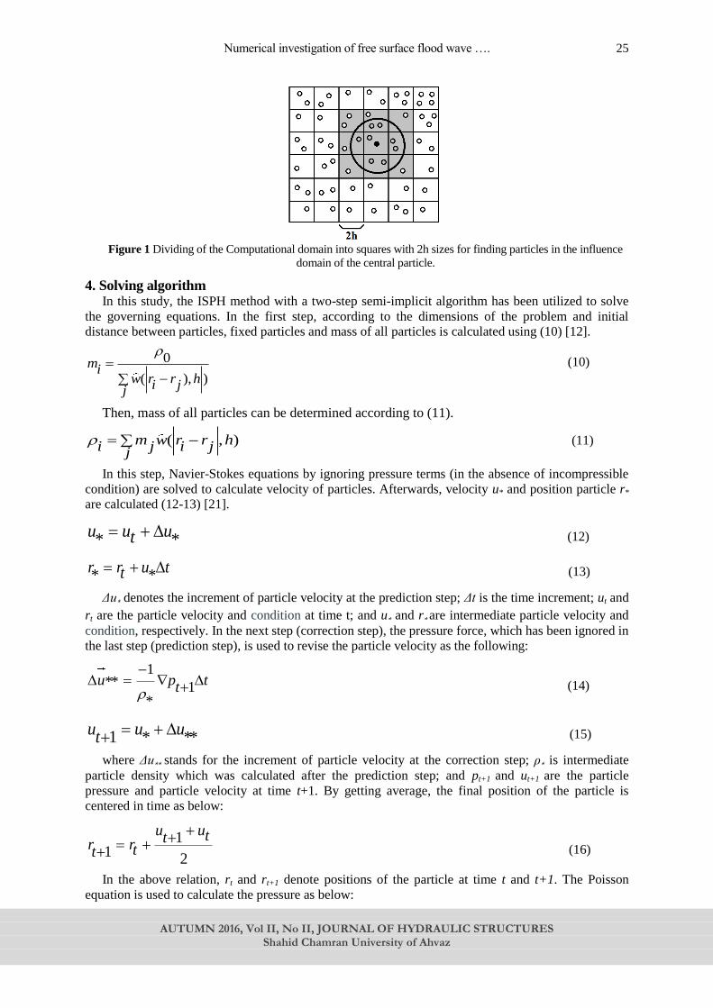
Figure 1 Dividing of the Computational domain into squares with 2h sizes for finding particles in the influence
domain of the central particle.
4. Solving algorithm In this study, the ISPH method with a two-step semi-implicit algorithm has been utilized to solve
the governing equations. In the first step, according to the dimensions of the problem and initial
distance between particles, fixed particles and mass of all particles is calculated using (10) [12].
0
( ), )mi
w r r hi jj
(10)
Then, mass of all particles can be determined according to (11).
( , )m w r r hi j i jj (11)
In this step, Navier-Stokes equations by ignoring pressure terms (in the absence of incompressible
condition) are solved to calculate velocity of particles. Afterwards, velocity u* and position particle r*
are calculated (12-13) [21].
* *u u ut (12)
* *r r u tt (13)
Δu⁎ denotes the increment of particle velocity at the prediction step; Δt is the time increment; ut and
rt are the particle velocity and condition at time t; and u⁎ and r⁎ are intermediate particle velocity and
condition, respectively. In the next step (correction step), the pressure force, which has been ignored in
the last step (prediction step), is used to revise the particle velocity as the following:
1** 1
*
u p tt
(14)
1 * **u u ut
(15)
where Δu⁎⁎ stands for the increment of particle velocity at the correction step; ρ⁎ is intermediate
particle density which was calculated after the prediction step; and pt+1 and ut+1 are the particle
pressure and particle velocity at time t+1. By getting average, the final position of the particle is
centered in time as below:
11
2
u uttr rtt
(16)
In the above relation, rt and rt+1 denote positions of the particle at time t and t+1. The Poisson
equation is used to calculate the pressure as below:
M. Zounemat-Kermani, H. Sheybanifard
AUTUMN 2016, Vol II, No II, JOURNAL OF HYDRAULIC STRUCTURES
Shahid Chamran University of Ahvaz
26
1 0 *.( )1 2
* 0
pt
t
(17)
Where ρ0 is initial constant density at each of the particles. The advantage of the ISPH method
is that large pressure fluctuations can be decreased because of using a strict hydrodynamic
formulation.
The pressure in (17) can be solved by either any available direct or iterative solvers. However,
the iterative solvers have shown to be more robust in case of great numbers of particles. 5. Boundary Conditions (solid walls and free surface) 5.1. Solid boundaries
For modelling solid wall, the solid impermeable boundaries are acted by unmoving wall particles.
They not only prevent the entrance of inner fluid particles into solid wall but also balance the pressure
of them. Because of the pressure balance of fluid particles, Poisson's equation will be solved for these
particles. It should be mentioned that two rows of dummy particles out of these walls are placed for
ignoring wall particles as free surface particles.
The velocities of wall particles are arranged zero to indicate the unmovable boundary condition.
5.2. Free surface In the ISPH model, the particle density is used to determine the free surface and after that, a
zero pressure is given to the free surface particles. Since there is no fluid particle existing in the
outside area of the free surface, thereafter the density on the surface particle should drop
significantly [17]. For recognizing free surface particles, if the calculated particle density satisfies
the following condition, the particle is recognized as a surface particle [5].
0* (18)
In (18), is free surface parameter and 0.8< <0.99. In this paper, =0.97 was used.
6. Modelling of free surface flows with ISPH model Three free surface problems have been considered to show the model's capabilities and to
investigate its accuracy. Two dam-break sudden and gradual flood wave problems and the solitary
wave in open-channel on a stiff bed are used to illustrate the model's capacity to calculate the free-
surface position and the distort of the water surface. The numerical results have been contrasted to
experimental measurements and analytical solution.
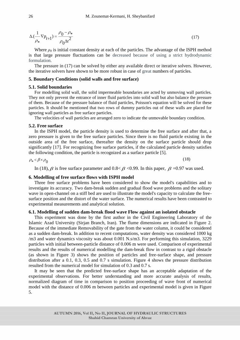
6.1. Modelling of sudden dam-break flood wave Flow against an isolated obstacle This experiment was done by the first author in the Civil Engineering Laboratory of the
Islamic Azad University (Sirjan Branch, Iran). The flume dimensions are indicated in Figure 2.
Because of the immediate Removability of the gate from the water column, it could be considered
as a sudden dam-break. In addition to recent computations, water density was considered 1000 kg
/m3 and water dynamics viscosity was about 0.001 N.s/m3. For performing this simulation, 3229
particles with initial between-particle distance of 0.006 m were used. Comparison of experimental
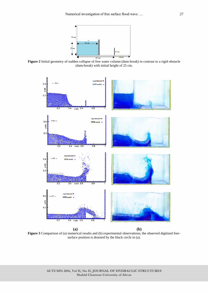
results and the results of numerical modelling the dam-break flow in contrast to a rigid obstacle
(as shown in Figure 3) shows the position of particles and free-surface shape, and pressure
distribution after a 0.1, 0.3, 0.5 and 0.7 s simulation. Figure 4 shows the pressure distribution
resulted from the numerical model for simulation of 0.3 and 0.7 s.
It may be seen that the predicted free-surface shape has an acceptable adaptation of the
experimental observations. For better understanding and more accurate analysis of results,
normalized diagram of time in comparison to position proceeding of wave front of numerical
model with the distance of 0.006 m between particles and experimental model is given in Figure
5.
Numerical investigation of free surface flood wave ….
AUTUMN 2016, Vol II, No II, JOURNAL OF HYDRAULIC STRUCTURES
Shahid Chamran University of Ahvaz
27
Figure 2 Initial geometry of sudden collapse of free water column (dam-break) in contrast to a rigid obstacle
(dam-break) with initial height of 25 cm.
(a) (b) Figure 3 Comparison of (a) numerical results and (b) experimental observations; the observed digitized free-
surface position is denoted by the black circle in (a).
M. Zounemat-Kermani, H. Sheybanifard
AUTUMN 2016, Vol II, No II, JOURNAL OF HYDRAULIC STRUCTURES
Shahid Chamran University of Ahvaz
28
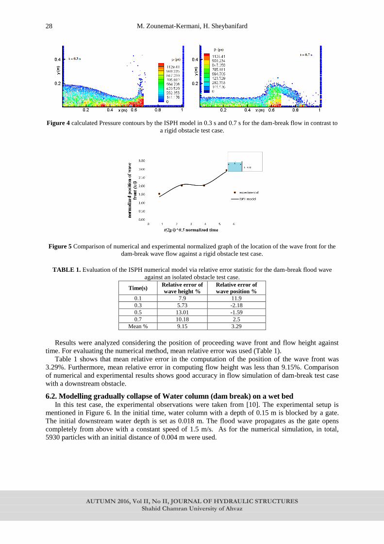
Figure 4 calculated Pressure contours by the ISPH model in 0.3 s and 0.7 s for the dam-break flow in contrast to
a rigid obstacle test case.
Figure 5 Comparison of numerical and experimental normalized graph of the location of the wave front for the
dam-break wave flow against a rigid obstacle test case.
TABLE 1. Evaluation of the ISPH numerical model via relative error statistic for the dam-break flood wave
against an isolated obstacle test case.
Time(s) Relative error of
wave height %
Relative error of
wave position %
0.1 7.9 11.9
0.3 5.73 -2.18
0.5 13.01 -1.59
0.7 10.18 2.5
Mean % 9.15 3.29
Results were analyzed considering the position of proceeding wave front and flow height against
time. For evaluating the numerical method, mean relative error was used (Table 1).
Table 1 shows that mean relative error in the computation of the position of the wave front was
3.29%. Furthermore, mean relative error in computing flow height was less than 9.15%. Comparison
of numerical and experimental results shows good accuracy in flow simulation of dam-break test case
with a downstream obstacle.
6.2. Modelling gradually collapse of Water column (dam break) on a wet bed In this test case, the experimental observations were taken from [10]. The experimental setup is
mentioned in Figure 6. In the initial time, water column with a depth of 0.15 m is blocked by a gate.
The initial downstream water depth is set as 0.018 m. The flood wave propagates as the gate opens
completely from above with a constant speed of 1.5 m/s. As for the numerical simulation, in total,
5930 particles with an initial distance of 0.004 m were used.
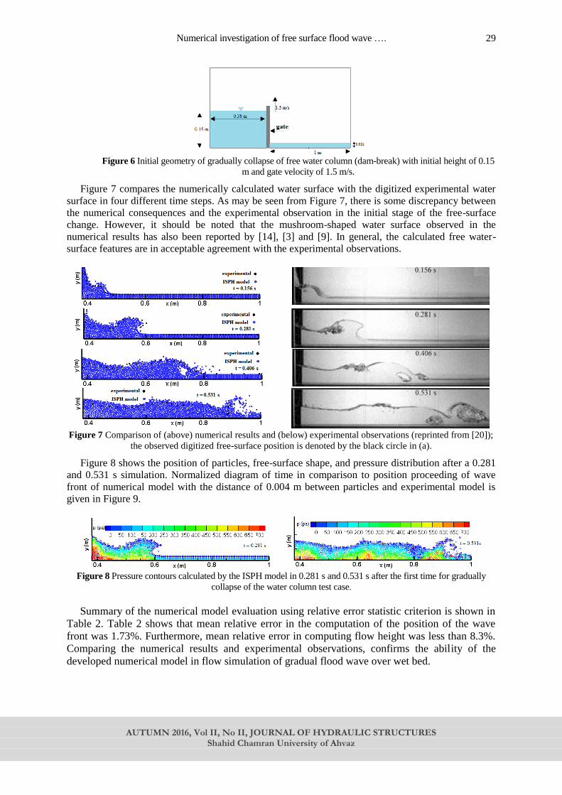
Numerical investigation of free surface flood wave ….
AUTUMN 2016, Vol II, No II, JOURNAL OF HYDRAULIC STRUCTURES
Shahid Chamran University of Ahvaz
29
Figure 6 Initial geometry of gradually collapse of free water column (dam-break) with initial height of 0.15
m and gate velocity of 1.5 m/s.
Figure 7 compares the numerically calculated water surface with the digitized experimental water
surface in four different time steps. As may be seen from Figure 7, there is some discrepancy between
the numerical consequences and the experimental observation in the initial stage of the free-surface
change. However, it should be noted that the mushroom-shaped water surface observed in the
numerical results has also been reported by [14], [3] and [9]. In general, the calculated free water-
surface features are in acceptable agreement with the experimental observations.
Figure 7 Comparison of (above) numerical results and (below) experimental observations (reprinted from [20]);
the observed digitized free-surface position is denoted by the black circle in (a).
Figure 8 shows the position of particles, free-surface shape, and pressure distribution after a 0.281
and 0.531 s simulation. Normalized diagram of time in comparison to position proceeding of wave
front of numerical model with the distance of 0.004 m between particles and experimental model is
given in Figure 9.
Figure 8 Pressure contours calculated by the ISPH model in 0.281 s and 0.531 s after the first time for gradually
collapse of the water column test case.
Summary of the numerical model evaluation using relative error statistic criterion is shown in
Table 2. Table 2 shows that mean relative error in the computation of the position of the wave
front was 1.73%. Furthermore, mean relative error in computing flow height was less than 8.3%.
Comparing the numerical results and experimental observations, confirms the ability of the
developed numerical model in flow simulation of gradual flood wave over wet bed.

M. Zounemat-Kermani, H. Sheybanifard
AUTUMN 2016, Vol II, No II, JOURNAL OF HYDRAULIC STRUCTURES
Shahid Chamran University of Ahvaz
30
Figure 9 Comparison of numerical and experimental normalized diagram of the position of the wave front for
gradually collapse of water column case.
TABLE 2 Evaluation of the ISPH numerical model via relative error statistic of the position of the wave front for
gradually collapse of water column test case. Time (s)
Relative error of
Wave height %
Relative error of
Wave position %
0.156 7.4 2.12
0.281 8.2 1.6
0.406 7.8 1.23
0.531 10 2.0
Mean % 8.3 1.73
6.3. Modeling of solitary wave In this part, the accuracy of ISPH flow model is assessed by analogizing the numerical and
theoretical wave heights of a solitary wave propagating on an isolated bed. Considering the following
relation (which is derived from the Boussinesq equation), the initial wave situation was arranged by
identifying the particles near the computational entrance regarding an analytical solitary wave profile
and velocity derived from the Boussinesq equation [21].
2
3
3( , ) sec [ ( )]
4
ax t a h x ct
d (19)
where η= water surface elevation, a=wave amplitude, d=water depth and ( )c g d a is the solitary
wave celerity. The horizontal velocity under the wave profile is calculated by (20)
gu
d (20)
In this study, a solitary wave with the wave amplitude a=0.06 m is considered. The water depth
is 0.2 m and the initial particle spacing is 0.01 m. The first situation was arranged by identifying
the particles near the computational entrance with the wave profile of Eq. (19), zero vertical
velocity and horizontal velocity of Eq. (20). As for the numerical computation, the 5200 particles
were placed on a regular grid with square cells, in a way that those that were above the profile
were eliminated. This condition leads to a slightly rough initial profile such that the fluid rapid
adjusts to the solitary wave profile. Figure 10 indicates the comparisons of the modeled wave
profiles and the analytical answers at various times.
0.00
0.50
1.00
1.50
2.00
2.50
3.00
0 2 4 6no
rma
lize
d p
osi
tio
n o
f
wa
ve
fro
nt
(x/l
) t(2g/l)^0.5 normalized time
experimental
ISPH model
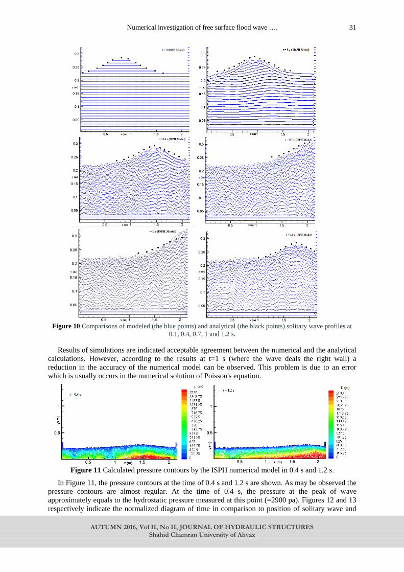
Numerical investigation of free surface flood wave ….
AUTUMN 2016, Vol II, No II, JOURNAL OF HYDRAULIC STRUCTURES
Shahid Chamran University of Ahvaz
31
Figure 10 Comparisons of modeled (the blue points) and analytical (the black points) solitary wave profiles at
0.1, 0.4, 0.7, 1 and 1.2 s.
Results of simulations are indicated acceptable agreement between the numerical and the analytical
calculations. However, according to the results at t=1 s (where the wave deals the right wall) a
reduction in the accuracy of the numerical model can be observed. This problem is due to an error
which is usually occurs in the numerical solution of Poisson's equation.
Figure 11 Calculated pressure contours by the ISPH numerical model in 0.4 s and 1.2 s.
In Figure 11, the pressure contours at the time of 0.4 s and 1.2 s are shown. As may be observed the
pressure contours are almost regular. At the time of 0.4 s, the pressure at the peak of wave
approximately equals to the hydrostatic pressure measured at this point (=2900 pa). Figures 12 and 13
respectively indicate the normalized diagram of time in comparison to position of solitary wave and
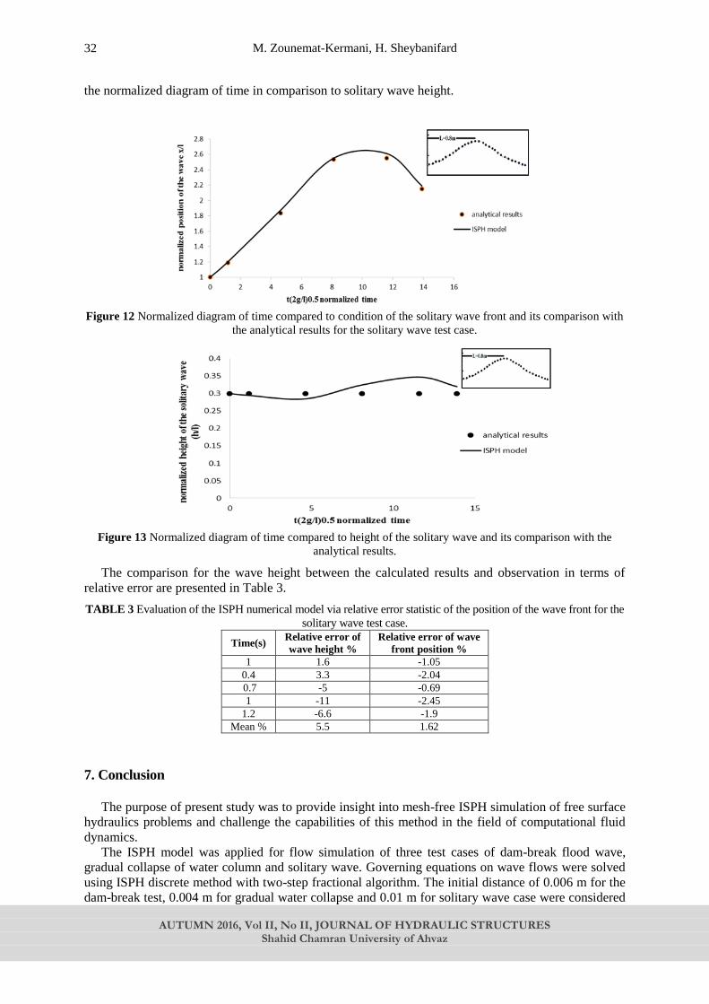
M. Zounemat-Kermani, H. Sheybanifard
AUTUMN 2016, Vol II, No II, JOURNAL OF HYDRAULIC STRUCTURES
Shahid Chamran University of Ahvaz
32
the normalized diagram of time in comparison to solitary wave height.
Figure 12 Normalized diagram of time compared to condition of the solitary wave front and its comparison with
the analytical results for the solitary wave test case.
Figure 13 Normalized diagram of time compared to height of the solitary wave and its comparison with the
analytical results.
The comparison for the wave height between the calculated results and observation in terms of
relative error are presented in Table 3.
TABLE 3 Evaluation of the ISPH numerical model via relative error statistic of the position of the wave front for the
solitary wave test case.
Time(s) Relative error of
wave height %
Relative error of wave
front position %
1 1.6 -1.05
0.4 3.3 -2.04
0.7 -5 -0.69
1 -11 -2.45
1.2 -6.6 -1.9
Mean % 5.5 1.62
7. Conclusion
The purpose of present study was to provide insight into mesh-free ISPH simulation of free surface
hydraulics problems and challenge the capabilities of this method in the field of computational fluid
dynamics.
The ISPH model was applied for flow simulation of three test cases of dam-break flood wave,
gradual collapse of water column and solitary wave. Governing equations on wave flows were solved
using ISPH discrete method with two-step fractional algorithm. The initial distance of 0.006 m for the
dam-break test, 0.004 m for gradual water collapse and 0.01 m for solitary wave case were considered
Numerical investigation of free surface flood wave ….
AUTUMN 2016, Vol II, No II, JOURNAL OF HYDRAULIC STRUCTURES
Shahid Chamran University of Ahvaz
33
between particles.
In order to assess the ability of the numerical method, mean relative error was used. The mean
relative error in the computation of the position of the wave front of the dam-break and water column
collapse were below 4%. Furthermore, mean relative error in computing flow height of these two cases
were below 10%. Moreover, the mean relative error in the computation of the height of the solitary
wave was 5.5% and mean relative error of Wave position was equal to 1.62 %. These outcomes
demonstrated the ability of the advanced model to deal with a realistic free-surface problem even when
large deformations exist in the free surface.
References
1. A. Shakibaeinia and Y. Jin, MPS-Based Mesh-Free Particle Method for Modeling Open-Channel
Flows, Hydraul. Eng J., 137(2011), pp. 1375–1384.
2. A. Colagrossi and M. Landrini, Numerical simulation of interfacial flows by smoothed particle
hydrodynamics, Comput. Phys J., 191(2003), pp. 448-475.
3. A.J.C. Crespo, M. Gómez-Gesteira and R.A. Dalrymple, Modeling dam break behavior over a wet
bed by a SPH technique, Waterw. Port Coastal Ocean Eng J., 134(2008), pp. 313–320.
4. B. Ataie-Ashtiani and G. Shobeyri, Numerical simulation of landslide impulsive waves by
incompressible smoothed particle hydrodynamics, Int. J. Numer. Methods Fluids., 56 (2008), pp.
209-232.
5. B. Ataie-Ashtiani, G. Shobeyri and L. Farhadi, Modified incompressible SPH method for simulating
free surface problems, Fluid Dyn. Res J., 40(2008), pp. 637-661.
6. C. Altomare, A.J.C. Crespo, J.M. Domínguez, M. Gómez-Gesteira, T. Suzuki and T. Verwaest,
Applicability of Smoothed Particle Hydrodynamics for estimation of sea wave impact on coastal
structures, Coastal Eng J., 96(2015), pp. 1-12.
7. E. Džebo, D. Žagar, M. Krzyk, M. Četina and G. Petkovšek, Different ways of defining wall shear
in smoothed particle hydrodynamics simulations of a dam-break wave, Hydraulic Research J.,
52(2014), pp. 453-464.
8. E. Fontaine, M. Landrini and M. Tulin, Breaking: Splashing and ploughing phases, Int. Workshop
on Waterwaves and Floating Bodies J., 4(2000), pp. 34 –38.
9. E.S. Lee, C. Moulinec, R. Xu, D. Violeau, D. Laurence and P. Stansby, Comparisons of weakly
compressible and truly incompressiblealgorithms for the SPH mesh free particle method, Comput.
Phys J., 227(2008), pp. 8417–8436.
10. I. Janosi M, D. Jan, K.G. Szabo and T. Tel, Turbulent drag reduction in dam-break flows, Exp.
Fluids J., 37(2004), pp. 219–229.
11. J.J. Monaghan, SPH without a tensile instability, Comput. Phys J, 159(2000), pp. 290-311.
12. J. Monaghan and A. Kos, Solitary waves on a Cretan beach, Waterw. Port Coastal Ocean Eng J.,
125(1999), pp. 145-155.
13. P. Jonsson, P. Jonsén, P. Andreasson, TS. Lundström, J. Gunnar and I. Hellström, Modelling Dam
Break Evolution over a Wet Bed with Smoothed Particle Hydrodynamics: A Parameter Study,
Engineering J., 7(2015), pp. 248-260.
14. P.K. Stansby, A. Chegini and T.C.D. Barnes, The initial stages of dam-break flow, Fluid Mech J.,
374(1998), pp. 407-424.
15. R.A. Dalrymple, O. Knio, Dn.T. Cox, M. Gesteira and S. Zou, Using a Lagrangian particle method
for deck overtopping, Proc., Waves J., (2002), pp. 1082–1091.
16. R. Gingold and J.J. Monaghan, Smoothed particle hydrodynamics: theory and application to non-
spherical stars, Mon. Not. R. Astron. Soc J., 181(1977), pp. 375-389.
17. R. Xu, P. Stansby and D. Laurence, Accuracy and stability in incompressible SPH (ISPH) based on
the projection method and a new approach, Comput. Phys J., 228(2009), pp. 6703-6725.
18. S. Lind, R. Xu, P.K. Stansby and B.D. Rogers, Incompressible smoothed particle hydrodynamics
for free-surface flows: A generalised diffusion-based algorithm for stability and validations for
impulsive flows and propagating waves, Comput. Phys J., 231(2012), pp. 1499–1523.

M. Zounemat-Kermani, H. Sheybanifard
AUTUMN 2016, Vol II, No II, JOURNAL OF HYDRAULIC STRUCTURES
Shahid Chamran University of Ahvaz
34
19. S. Lind, P.K. Stansby and B.D. Rogers and P.M. Lloyd, Numerical predictions of water–air wave
slam using incompressible–compressible smoothed particle hydrodynamics, Appl. Ocean Res J.,
49(2015), pp. 57-71.
20. S. Shao and E.Y. Lo, Incompressible SPH method for simulating Newtonian and non-Newtonian
flows with a free surface, Adv. Water Resour J., 26(2003), pp. 787-800.
21. S. Shao, Incompressible SPH flow model for wave interactions with porous media, Coastal Eng J.,
57(2010), pp. 304-316.
AUTUMN 2016, Vol II, No II, JOURNAL OF HYDRAULIC STRUCTURES
Shahid Chamran University of Ahvaz
Journal of Hydraulic Structures
J. Hydraul. Struct., 2016; 2(2):35-45
DOI: 10.22055/jhs.2016.12850
Hydrological Assessment of Daily Satellite Precipitation
Products over a Basin in Iran
Saber Moazami1
Arman Abdollahipour2
Mahmoud Zakeri Niri3
Seyed Mohammad Ashrafi4
Abstract In order to measure precipitation as the main variable for estimating the runoff and designing
hydraulic structures, the satellite algorithm products that have the proper spatial and temporal
coverage, can be used. In this study, at first, the daily streamflow simulation of Sarough-Cahy
River from the Zarinehroud basin was conducted through the artificial neural network (ANN)
and ground data of daily precipitation, temperature and discharge for the years of 1988 to 2008.
The developed network was trained, validated and tested. Then, in order to evaluate the products
of satellite precipitation algorithms in streamflow simulation which is the aim of this study, daily
satellite rainfall data of PERSIANN, TMPA-3B42V7, TMPA-3B42RT and CMORPH between
2003 and 2008 were used as an input data to the trained ANN model. Considering indices of R2,
RMSE and MAE implemented for evaluations, the results indicated that satellite rainfall
algorithms are able to simulate runoff efficiently over the study area.
Keywords: Satellite Precipitation Products (SPPs), Simulation, Daily streamflow, Artificial
Neural Networks (ANNs), Basin
Received: 17 July 2016; Accepted: 08 November 2016
1. Introduction Since the most catchments of Iran country lack of hydrometric stations with long-term data,
using methods that help them in estimating runoff from precipitation is of considerable
1
Assisstant Professor, Environmental Sciences Research Center, Department of Civil Engineering,
Islamshahr Branch, Islamic Azad University, Islamshahr, Tehran, Iran, [email protected]
(Corresponding author) 2 Ph.D Student, Department of Civil Engineering, Roudehen Branch, Islamic Azad university, Roudehen,
Tehran, Iran, [email protected] 3 Assisstant Professor, Environmental Sciences Research Center, Department of Civil Engineering,
Islamshahr Branch, Islamic Azad University, Islamshahr, Tehran, Iran, [email protected] 4
Assisstant Professor, Department of Civil Engineering, Faculty of Engineering, Shahid Chamran
University of Ahvaz, Ahvaz, Iran, [email protected]
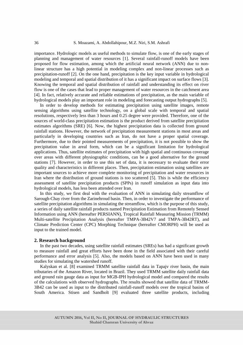
S. Moazami, A. Abdollahipour, M.Z. Niri, S.M. Ashrafi
AUTUMN 2016, Vol II, No II, JOURNAL OF HYDRAULIC STRUCTURES
Shahid Chamran University of Ahvaz
36
importance. Hydrologic models as useful methods to simulate flow, is one of the early stages of
planning and management of water resources [1]. Several rainfall-runoff models have been
proposed for flow estimation, among which the artificial neural network (ANN) due to non-
linear structure has a high potential in modeling complex and non-linear processes such as
precipitation-runoff [2]. On the one hand, precipitation is the key input variable in hydrological
modeling and temporal and spatial distribution of it has a significant impact on surface flows [3].
Knowing the temporal and spatial distribution of rainfall and understanding its effect on river
flow is one of the cases that lead to proper management of water resources in the catchment area
[4]. In fact, relatively accurate and reliable estimations of precipitation, as the main variable of
hydrological models play an important role in modeling and forecasting output hydrographs [5].
In order to develop methods for estimating precipitation using satellite images, remote
sensing algorithms using satellite technology, on a global scale with temporal and spatial
resolutions, respectively less than 3 hours and 0.25 degree were provided. Therefore, one of the
sources of world-class precipitation estimation is the product derived from satellite precipitation
estimates algorithms (SRE) [6]. Now, the highest precipitation data is collected from ground
rainfall stations. However, the network of precipitation measurement stations in most areas and
particularly in developing countries such as Iran, do not have a proper spatial coverage.
Furthermore, due to their pointed measurements of precipitation, it is not possible to show the
precipitation value in areal form, which can be a significant limitation for hydrological
applications. Thus, satellite estimates of precipitation with high spatial and continuous coverage
over areas with different physiographic conditions, can be a good alternative for the ground
stations [7]. However, in order to use this set of data, it is necessary to evaluate their error
quality and characteristics in different places. Then, precipitation estimation using satellites are
important sources to achieve more complete monitoring of precipitation and water resources in
Iran where the distribution of ground stations is too scattered [5]. This is while the efficiency
assessment of satellite precipitation products (SPPs) in runoff simulation as input data into
hydrological models, has less been attended over Iran.
In this study, we first deal with the evaluation of ANN in simulating daily streamflow of
Sarough-Chay river from the Zarinehroud basin. Then, in order to investigate the performance of
satellite precipitation algorithms in simulating the streamflow, which is the purpose of this study,
a series of daily satellite rainfall products named Precipitation Estimation from Remotely Sensed
Information using ANN (hereafter PERSIANN), Tropical Rainfall Measuring Mission (TRMM)
Multi-satellite Precipitation Analysis (hereafter TMPA-3B42V7 and TMPA-3B42RT), and
Climate Prediction Center (CPC) Morphing Technique (hereafter CMORPH) will be used as
input to the trained model.
2. Research background In the past two decades, using satellite rainfall estimates (SREs) has had a significant growth
to measure rainfall and great efforts have been done in the field associated with their careful
performance and error analysis [5]. Also, the models based on ANN have been used in many
studies for simulating the watershed runoff.
Kalyskan et al. [8] examined TRMM satellite rainfall data in Tapajv river basin, the main
tributaries of the Amazon River, located in Brazil. They used TRMM satellite daily rainfall data
and ground rain gauge data as input for MGB-IPH hydrological model and compared the results
of the calculations with observed hydrographs. The results showed that satellite data of TRMM-
3B42 can be used as input to the distributed rainfall-runoff models over the tropical basins of
South America. Stisen and Sandholt [9] evaluated three satellite products, including

Hydrological assessment of daily satellite precipitation ….
AUTUMN 2016, Vol II, No II, JOURNAL OF HYDRAULIC STRUCTURES
Shahid Chamran University of Ahvaz
37
PERSIANN, CMORPH and TRMM-3B42 as input in MIKE SHE hydrological model over the
Senegal river basin and found that the performance of TRMM -3B42 is better than other satellite
products .
Behrangi et al. [10] evaluated the efficacy of satellite precipitation products (SPPs) to
simulate runoff at the basin scale. For this purpose, five products of satellite algorithms named
TMPA-RT, TMPA-V6, CMORPH, PERSIANN and PERSIANN-adj were implemented as
inputs to SAC-SMA hydrological model in order to simulate the runoff in monthly and 6 hours
scales. The results for all five kinds of products in different rainfall intensities as well as
different seasons were compared with each other and the ability of each product to capture the
runoff with respect to its errors and uncertainties was expressed.
Lee et al. [11] compared TRMM satellite rainfall data with rain gauge data at different time
scales and evaluated the performance of TRMM data to simulate hydrological processes in
Yangtze river basin of Znjyng in China. Simulation of monthly hydrological processes showed
that TRMM satellite rainfall data can be useful for simulating the flow over the basin. Moazami
et al. [5] compared three satellite rainfall estimation algorithms (PERSIANN, TMPA-3B42V7
and TMAP-3B42RT) with rain-gauge data over the whole country of Iran and , concluded that
TMPA-3B42V7 product with values of Mbias =-1/47 mmd-1
, RBias= -13.6%, MAE = 4.5,
RMSE = 6.5 mmd-1 , and correlation coefficient of 0.61 represents better estimates of daily
precipitation than two other products.
Dawson and Willlbay [12], Tokar and Johnson [13], Tokar and Marcus [2], and Zhang [14],
have also acknowledged the ability of ANNs to model the non-linear phenomena. Tokar and
Marcus [2] compared the ANN and conceptual models to estimate the runoff of Fraser river
watershed in Colorado. They reported the accuracy of achievement to an appropriate answer for
predicting the runoff in the neural network compared to conceptual models. Soltani [15] by
comparing the performance of conceptual models and ANN in simulating the rainfall-runoff
process concluded that neural network requires less information and also is calibrated and
verified faster compared to other models.
3. Materials and Methods
3.1. Study area
Zarinehroud basin (45-̊45 to 15-̊47 east longitude and 30- ̊35 to 45-̊36 north latitude) with
an approximate area of 11841 km2 is widespread in the southeast of Urmia Lake in
northwestern part of Iran. In this research, Sarough-Chay river sub-basin of Zarinehroud was
chosen with area of 2403.8 km2, due to completeness of its rain gauge data named TAKAB
and its hydrometric station named Safakhaneh (See Figure 1).
3.2. Data Ground data of daily rainfall, average temperature and discharge from 1988 to 2008 have
been used to simulate the streamflow in this study. The first 10 years from 23/09/1988 to
22/09/1998 is intended for training the proposed ANN model, the 5 years from 23/09/1998 to
22/09/2003 for the validation, and the rest 5 years from 23/09/2003 to 21/9/ 2008 for testing the
model. The daily precipitation data of PERSIANN, TMPA-3B42V7, TMPA-3B42RT and
CMORPH products were derived through the aggregation of 3-hour time resolution. However,
the spatial scale of satellite data is in square pixel size with 0.25 degree, thus, a rainfall value for
each satellite product is obtained at each pixel [5]. Figure 2 shows the pixels network over the
whole country of Iran which composed of 0.25 degree pixels.
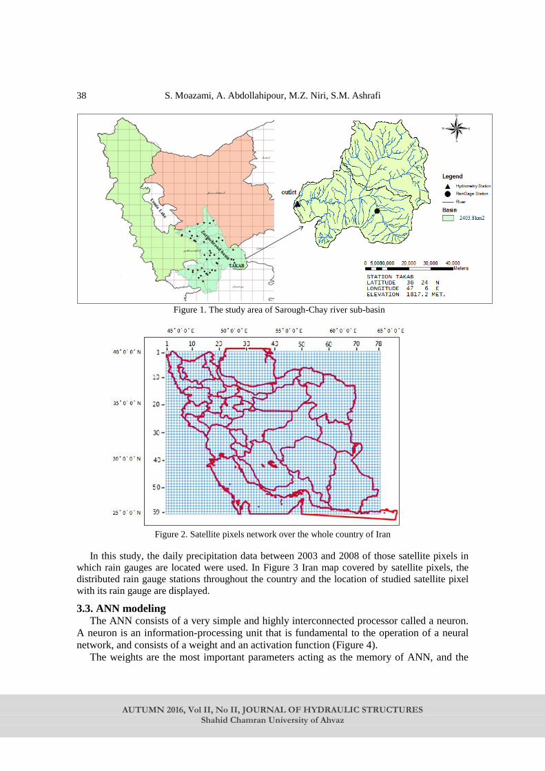
S. Moazami, A. Abdollahipour, M.Z. Niri, S.M. Ashrafi
AUTUMN 2016, Vol II, No II, JOURNAL OF HYDRAULIC STRUCTURES
Shahid Chamran University of Ahvaz
38
Figure 1. The study area of Sarough-Chay river sub-basin
Figure 2. Satellite pixels network over the whole country of Iran
In this study, the daily precipitation data between 2003 and 2008 of those satellite pixels in
which rain gauges are located were used. In Figure 3 Iran map covered by satellite pixels, the
distributed rain gauge stations throughout the country and the location of studied satellite pixel
with its rain gauge are displayed.
3.3. ANN modeling The ANN consists of a very simple and highly interconnected processor called a neuron.
A neuron is an information-processing unit that is fundamental to the operation of a neural
network, and consists of a weight and an activation function (Figure 4).
The weights are the most important parameters acting as the memory of ANN, and the
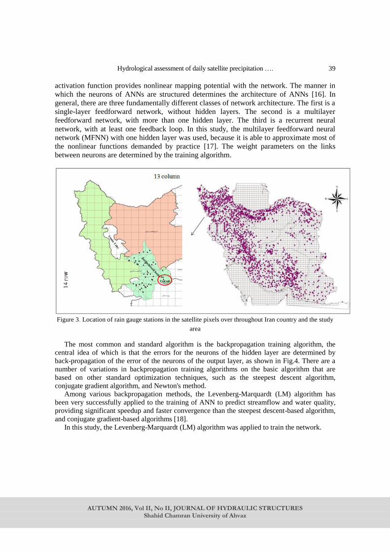
Hydrological assessment of daily satellite precipitation ….
AUTUMN 2016, Vol II, No II, JOURNAL OF HYDRAULIC STRUCTURES
Shahid Chamran University of Ahvaz
39
activation function provides nonlinear mapping potential with the network. The manner in
which the neurons of ANNs are structured determines the architecture of ANNs [16]. In
general, there are three fundamentally different classes of network architecture. The first is a
single-layer feedforward network, without hidden layers. The second is a multilayer
feedforward network, with more than one hidden layer. The third is a recurrent neural
network, with at least one feedback loop. In this study, the multilayer feedforward neural
network (MFNN) with one hidden layer was used, because it is able to approximate most of
the nonlinear functions demanded by practice [17]. The weight parameters on the links
between neurons are determined by the training algorithm.
Figure 3. Location of rain gauge stations in the satellite pixels over throughout Iran country and the study
area
The most common and standard algorithm is the backpropagation training algorithm, the
central idea of which is that the errors for the neurons of the hidden layer are determined by
back-propagation of the error of the neurons of the output layer, as shown in Fig.4. There are a
number of variations in backpropagation training algorithms on the basic algorithm that are
based on other standard optimization techniques, such as the steepest descent algorithm,
conjugate gradient algorithm, and Newton's method.
Among various backpropagation methods, the Levenberg-Marquardt (LM) algorithm has
been very successfully applied to the training of ANN to predict streamflow and water quality,
providing significant speedup and faster convergence than the steepest descent-based algorithm,
and conjugate gradient-based algorithms [18].
In this study, the Levenberg-Marquardt (LM) algorithm was applied to train the network.
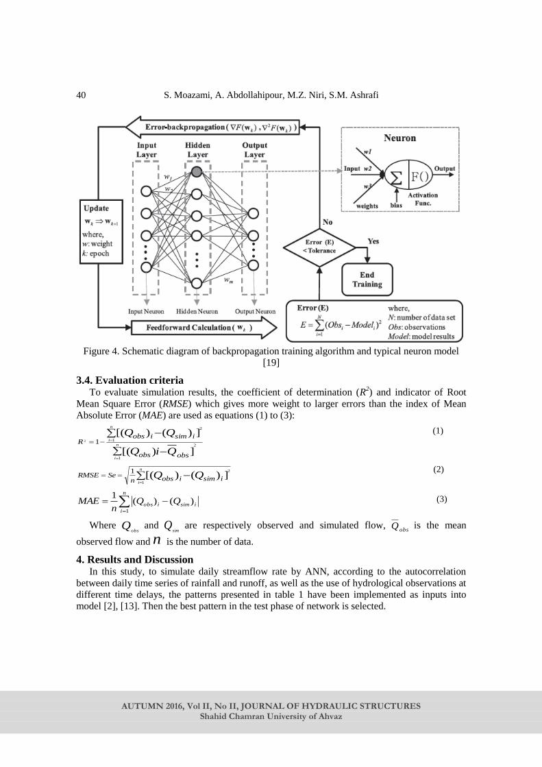
S. Moazami, A. Abdollahipour, M.Z. Niri, S.M. Ashrafi
AUTUMN 2016, Vol II, No II, JOURNAL OF HYDRAULIC STRUCTURES
Shahid Chamran University of Ahvaz
40
Figure 4. Schematic diagram of backpropagation training algorithm and typical neuron model
[19] 3.4. Evaluation criteria
To evaluate simulation results, the coefficient of determination (R2) and indicator of Root
Mean Square Error (RMSE) which gives more weight to larger errors than the index of Mean
Absolute Error (MAE) are used as equations (1) to (3):
n
i
n
i
obsobs
isimiobsR
QiQ
1
2
1
2
])[(
])()[(12
(1)
n
iisimiobsn
SeRMSE QQ1
2
])()[(1 (2)
n
i
isimiobs QQn
MAE1
)()(1 (3)
Where Qobs
and Qsim
are respectively observed and simulated flow, obs
Q is the mean
observed flow and n is the number of data.
4. Results and Discussion In this study, to simulate daily streamflow rate by ANN, according to the autocorrelation
between daily time series of rainfall and runoff, as well as the use of hydrological observations at
different time delays, the patterns presented in table 1 have been implemented as inputs into
model [2], [13]. Then the best pattern in the test phase of network is selected.

Hydrological assessment of daily satellite precipitation ….
AUTUMN 2016, Vol II, No II, JOURNAL OF HYDRAULIC STRUCTURES
Shahid Chamran University of Ahvaz
41
Table 1. The patterns used as inputs to the ANN model
Q(t) = f ( P(t-1) , P(t) , T(t) ) Model 1
Q(t) = f ( P(t-1) , P(t) , Q(t-1) ) Model 2
Q(t) = f ( P(t-1) , P(t) , T(t) , Q(t-1) ) Model 3
Q(t) = f ( P(t-2) , P(t-1) , P(t) , T(t) ) Model 4
Q(t) = f ( P(t-2) , P(t-1) , P(t) , Q(t-1) ) Model 5
Q(t) = f ( P(t-2) , P(t-1) , P(t) , T(t) , Q(t-1) ) Model 6
Q(t) = f ( P(t-3) , P(t-2) , P(t-1) , P(t) , Q(t-1) ) Model 7
Where, indicates the daily discharge, height of daily rainfall, mean daily temperature
of basin, and time step of calculations by model.
In this method, a three-layer Perceptron and training function propagation model were used.
Using trial and error, the number of neurons in the middle layer and the number of repetitions
was obtained in order to achieve optimal function with the aim of minimizing the error factor.
The activation function of the middle layer is Logsig (hidden layer with 10 neurons) and the
output layer activation function is Purelin neuron linear function with the number of outlets. And
also due to the use of stimulant function Logsig, the data were normalized between (1 and 0).
The results of network assessment in the test phase with the input patterns are shown in Table 2.
Table 2. Evaluation ANN with various input patterns during network testing
R2
Se/Sy Se Sy
Evaluation
Models
0.15 0.59 6.20 10.33 Model 1
0.77 0.41 4.79 11.70 Model 2
0.78 0.36 3.71 10.33 Model 3
0.21 0.54 5.55 10.33 Model 4
0.91 0.29 3.49 11.88 Model 5
0.88 0.33 3.45 10.33 Model 6
0.90 0.31 3.59 11.98 Model 7
Where Sy is Standard Division of flow observations, Se is root mean square error and R2
represents the coefficient of determination between observed and simulated discharges. If Se is
significantly smaller than Sy, the model will provide an accurate prediction. Conversely, if Se is
equal to or greater than Sy, the model prediction will not be accurate [2]. Therefore, the less ratio
of Se/Sy leads to the higher accuracy of streamflow prediction by model [13]. According to the
values expressed in table 2, the input pattern of No. 5 in the network test phase as well over the
study area was superior to other patterns and hence is selected as the final pattern. Furthermore,
in order to evaluate the efficiency of satellite-based precipitation estimate algorithms using
evaluation criteria, daily precipitation derived from PERSIANN, TMPA-3B42V7, TMPA-
3B42RT and CMORPH were used as input to trained network instead of rain gauge data to
Q P T
t
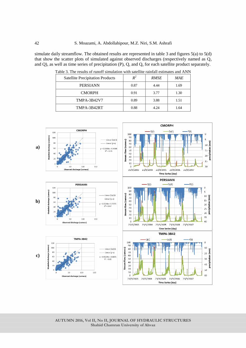
S. Moazami, A. Abdollahipour, M.Z. Niri, S.M. Ashrafi
AUTUMN 2016, Vol II, No II, JOURNAL OF HYDRAULIC STRUCTURES
Shahid Chamran University of Ahvaz
42
simulate daily streamflow. The obtained results are represented in table 3 and figures 5(a) to 5(d)
that show the scatter plots of simulated against observed discharges (respectively named as Qs
and Q), as well as time series of precipitation (P), Q, and Qs for each satellite product separately.
Table 3. The results of runoff simulation with satellite rainfall estimates and ANN
MAE RMSE R2 Satellite Precipitation Products
1.69 4.44 0.87 PERSIANN 1.30 3.77 0.91 CMORPH 1.51 3.88 0.89 TMPA-3B42V7 1.64 4.24 0.88 TMPA-3B42RT
a)
b)
c)
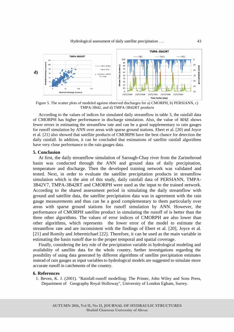
Hydrological assessment of daily satellite precipitation ….
AUTUMN 2016, Vol II, No II, JOURNAL OF HYDRAULIC STRUCTURES
Shahid Chamran University of Ahvaz
43
d)
Figure 5. The scatter plots of modeled against observed discharges for a) CMORPH, b) PERSIANN, c)
TMPA-3B42, and d) TMPA-3B42RT products
According to the values of indices for simulated daily streamflow in table 3, the rainfall data
of CMORPH has higher performance in discharge simulation. Also, the value of MAE shows
fewer errors in estimating the streamflow rate and can be a good supplementary to rain gauges
for runoff simulation by ANN over areas with sparse ground stations. Ebert et al. [20] and Joyce
et al. [21] also showed that satellite products of CMORPH have the best chance for detection the
daily rainfall. In addition, it can be concluded that estimations of satellite rainfall algorithms
have very close performance to the rain gauges data.
5. Conclusion
At first, the daily streamflow simulation of Sarough-Chay river from the Zarinehroud
basin was conducted through the ANN and ground data of daily precipitation,
temperature and discharge. Then the developed training network was validated and
tested. Next, in order to evaluate the satellite precipitation products in streamflow
simulation which is the aim of this study, daily rainfall data of PERSIANN, TMPA-
3B42V7, TMPA-3B42RT and CMORPH were used as the input to the trained network.
According to the shared assessment period in simulating the daily streamflow with
ground and satellite data, the satellite precipitation data was in agreement with the rain
gauge measurements and thus can be a good complementary to them particularly over
areas with sparse ground stations for runoff simulation by ANN. However, the
performance of CMORPH satellite product in simulating the runoff of is better than the
three other algorithms. The values of error indices of CMORPH are also lower than
other algorithms, which represents the lower error of the model to estimate the
streamflow rate and are inconsistent with the findings of Ebert et al. [20], Joyce et al.
[21] and Romily and Jebermichael [22]. Therefore, it can be used as the main variable in
estimating the basin runoff due to the proper temporal and spatial coverage. Finally, considering the key role of the precipitation variable in hydrological modeling and
availability of satellite data for the whole country, further investigations regarding the
possibility of using data generated by different algorithms of satellite precipitation estimates
instead of rain gauges as input variables to hydrological models are suggested to simulate more
accurate runoff in catchments of the country.
6. References 1. Beven, K. J. (2001). "Rainfall-runoff modelling: The Primer, John Wiley and Sons Press,
Department of Geography Royal Holloway", University of London Egham, Surrey.
S. Moazami, A. Abdollahipour, M.Z. Niri, S.M. Ashrafi
AUTUMN 2016, Vol II, No II, JOURNAL OF HYDRAULIC STRUCTURES
Shahid Chamran University of Ahvaz
44
2. Tokar, A.S. and Markus M. (2000). "Precipitation-runoff modeling using artificial neural
networks and conceptual models", Journal of Hydrologic Engineering, Vol.5, April,
PP.156-161.
3. Li, X and Zhang Q, Xu Ch. (2013). "Assessing the performance of satellite based
precipitation products and its dependence on topography over Poyang Lake basin", Theor
Appl Climatol, 115:713–729.
4. Sadeghi, S. H. R., Yasrebi, B., Noormohammadi F., (2005). "Preparation and analysis of
precipitation - runoff models, Haraz catchment monthly in Mazandaran", Journal of
Agricultural Sciences and Natural Resources of the Caspian Sea, 3 (1): 1-12. (In Persian)
5. Moazami S, Golian S, Kavianpour M R and Hong Y. (2013). "Comparison of PERSIANN
and V7 TRMM Multi-satellite Precipitation Analysis (TMPA) products with rain gauge
data over Iran", International Journal.
6. Katiraie Boroujerdi, P. S. (2013). "Comparison of monthly satellite and ground precipitation
data in a network of high-resolution on Iran," Iranian Geophysical Journal, Volume 7, Issue
4, Pp. 149-160. (In Persian) 7. Baranizadeh, A., Behiar, M. B., Javanmard, S., Abedini, Y. (2011). "Validation of
precipitation algorithm of PERSIANN satellite through (APHRODITE) reticulated ground
precipitation in Iran", the article of physics conference in Iran, interdisciplinary physics,
2615-2618. (In Persian)
8. Collischonn B, Collischonn W and Morelli Tucci C E, (2008). "Daily hydrological modeling
in the Amazon basin using TRMM rainfall estimates", Journal of Hydrology, 360: 207-216.
9. Stisen S and Sandholt I, (2010). "Evaluation of remote-sensing-based rainfall products
through predictive capability in hydrological runoff modeling", Journal of Hydrology
Process, 24(7):879–891.
10. Behrangi A, Khakbaz B, Jaw TC, AghaKouchak A, Hsu K and Sorooshian S, (2011).
"Hydrologic evaluation of satellite precipitation products over a mid-size basin", Journal of
Hydrology, 397:225–237.
11. Li X and Zhang Q, Xu Ch, (2012). "Suitability of the TRMM satellite rainfalls in driving a
distributed hydrological model for water balance computations in Xinjiang catchment,
Poyang lake basin", Journal of Hydrology, 426- 427:28-38.
12. Dawson C.W. and Wilby R., (1988). "An artificial neural network approach for rainfall-
runoff modeling", Hydrological Sciences Journal, Vol.43, February, PP. 47-66.
13. Tokar A.S. and Johnson P.A., (1999). "Rainfall-runoff modeling using artificial neural
networks", Journal of Hydrologic Engineering, Vol.4, July , PP.232-239.
14. Zhang B. and Govindaraju R.S. (2003). "Geomorphology-based artificial neural networks
(GANNs) for estimation of direct runoff over watersheds", Journal of Hydrologic
Engineering, Vol.273, October, PP. 18-34.
15. Soltani, S., (2002), "Comparison of conceptual models with Artificial Neural Networks in
simulating precipitation - runoff", Master Thesis, Tarbiat Modarres University, Tehran. (In
Persian)
16. Haykin, S., 1999. Neural Networks : a Comprehensive Foundation, second ed. Prentice

Hydrological assessment of daily satellite precipitation ….
AUTUMN 2016, Vol II, No II, JOURNAL OF HYDRAULIC STRUCTURES
Shahid Chamran University of Ahvaz
45
Hall, Upper Saddle River, N.J., USA, p. 842.
17. Mulia, I.E., Tay, H., Roopsekhar, K., Tkalich, P., 2013. Hybrid ANN-GA model for
predicting turbidity and chlorophyll-a concentration. J. Hydro environ. Res. 7, 279-299.
18. Zamani, A., Azimian, A., Heemink, A., Solomatine, D., 2009. Wave height prediction at
the Caspian Sea using a data-driven model and ensemble-based data assimilation methods.
J. Hydroinform. 11 (2), 154-164.
19. Sung, E. K. and Il Won, S. (2015). “Artificial Neural Network ensemble modeling with
conjunctive data clustering for water quality prediction in rivers”, Journal of Hydro-
environment Research 9, 325-339.
20. Ebert, E. E., Janowiak, J.E., and Kidd, C. (2007). "Comparison of near-real-time
precipitation estimates from satellite observations and numerical models", Bull. Amer.
Meteor. Soc., 88, 47-64.
21. Joyce, R. J., Janowiak, J. E., Arkin, P. A. and Xie, P. (2004), "CMORPH: A method that
produces global precipitation estimates from passive microwave and infrared data at high
spatial and temporal resolution", Journal of Hydrometeorol, 5:487-503.
22. Romilly T.G., Gebremichael M., (2011), Evaluation of satellite rainfall estimates over
Ethiopian river basins, EGU, Hydrology and Earth System Sciences, 15:1505-1514.
AUTUMN 2016, Vol II, No II, JOURNAL OF HYDRAULIC STRUCTURES
Shahid Chamran University of Ahvaz
Journal of Hydraulic Structures
J. Hydraul. Struct., 2016; 2(2):46-61
DOI: 10.22055/jhs.2016.12856
Numerical Simulation of Flow Pattern around the Bridge Pier
with Submerged Vanes
Sajedeh Haji Azizi1
Davood Farsadizadeh2
Hadi Arvanaghi3
Akram Abbaspour4
Abstract Bridges are very important for establishing communication paths. For this reason, it is important
to control scour around bridge piers. Several methods have been proposed for scour control. One
of the most useful methods is the use of submerged vanes. In the other hand, laboratory
circumstances force many considered effective factors to be skipped in the scour phenomenon.
In this situation, the importance of using numerical models would appear even more. In this
research, numerical simulation of the flow pattern around the piers surrounded by submerged
vanes has been carried out. For this purpose, the structure simulated in three dimensions using
Fluent software. K-ε turbulence model with VOF and mixture models for multiphase flow
simulation were applied. Afterward analysis of the water surface profiles, velocity distribution
profiles, and shear tension of the bed in multiple placements conditions including multiple vanes
within two flow intensity and two different angles were performed. The results showed that there
is a good agreement between numerical and experimental results. The best models in this
research were found to be Realizable k-ε turbulence model with VOF multiphase model for
water surface profile and velocity distribution profiles. The maximum extracted relative errors
for water surface profiles and velocity distribution profiles were 2.23% and 2.92%, respectively.
Also, analysis of the counts and placement angles showed that 6 vanes rather to 2 and 4 vanes
and also angle of 30 degrees rather to angle of 20 degree performs better in action. The other
results of this study, are no change in water surface profiles, reduction of the velocity and the
amount of shear stress around the piers in different placement conditions including multiple
submerged vanes.
Keywords: Scouring, Flow pattern, Bridge pier, Numerical simulation, Submerged vanes
Received: 06 September 2016; Accepted: 15 November 2016
1 Department of Water Engineering, University of Tabriz, Tabriz, 09371676441, [email protected]
(Corresponding author) 2
Associate Professor, Department of Water Engineering, University of Tabriz, Tabriz,
[email protected] 3Assistant Professor, Department of Water Engineering, University of Tabriz, Tabriz, [email protected]
4 Assistant Professor, Department of Water Engineering, University of Tabriz, Tabriz,
Numerical Simulation of Flow Pattern around the Bridge ….
AUTUMN 2016, Vol II, No II, JOURNAL OF HYDRAULIC STRUCTURES
Shahid Chamran University of Ahvaz
47
1. Introduction Bridges are the most important structures of communication which are always subject to
degradation. In studies, scour is considered as one of the main reasons of destruction. submerged
vanes are used to control the size of the scour hole and to protect the structures. Numerical
Study of submerged vanes would be possible by a closer look. Marelius and sinha (1998)
experimentally and numerically studied velocity profile around the submerged vanes.
Hassanzadeh et al (2006) have developed a numerical model to simulate the flow pattern around
bridge piers. Ariyanfar and Shafai Bajestan (2008) numerically studied the flow pattern around
the base of the cylindrical piers using Fluent model. Besharati Givi and Hakim Zadeh (2009)
simulated cylindrical pier in models three dimensions using Fluent software. Alamatiyan and
Jafarzadeh (2009) they studied the numerical model of flow conditions around the bridge piers.
Sarveram et al (2008) studied the numerical simulation and flow velocity distribution around
bridge pier. Kariminia and Salehi Neyshabouri (2011) simulated the backwater phenomenon for
bridge pier using Fluent software. Asadi Partov et al (2012) studied numerical simulation of flow
pattern in a direct channel and the effect of bridge pier diameter on it. Kalali et al (2012) studied
the numerical simulation of the flow pattern around slant bridge piers. Hoshmand et al (2013)
studied three-dimensional numerical modeling of the flow around the bridge pier in meandering
beds. Yen et al (2001) simulated bed change and flow pattern in the cylindrical bridge pier using
Flow-3D software and a combination of three-dimensional flow model and scour model.
Roulund et al (2002) simulated flow around bridge pier by three-dimensional numerical model.
In the present study, the flow pattern around bridge piers including submerged vanes simulated
and assessed. This study was carried out with a CFD program, which uses the finite volume
method to solve 3D Reynolds averaged Navier Stokes (RANS) equations for this model. The
free surface levels computed using VOF (volume-of-fluid) method and compared with
experimental data.
2. Materials and Methods 2.1. Experimental Procedure
The experiments carried out by Shojaei (2009) in a metal glass flume with a rectangular cross-
section. The flume was 0.8 m wide, 0.5 m deep and 8 m long. The slope of the channel was 0.001.
A cylindrical steel pipe with diameter of 0.06 m used to model the pier. Submerged vanes models
made in rectangular square form. The submerged vanes was 0.001 m wide, 0.03 m deep and 0.09
m long. The discharge was measured by a rectangular weir placed at the end of channel. Fig. 1
shows the submerged vanes and the pier parameters. In all experiments, according to the
calculations u∗ u∗c⁄ = 0.9 , flow depth equaled to 0.147 m and discharge is considered
0.03 m3 sec⁄ . Also, with depth of 0.147 m has been considered which is the required condition in
order to avoid flow depth affecting on scour hole depth. In all experiments, the flow was turbulent.
The recognition criterion in this type of flows is Reynolds number, which is defined as Re =VR
ν⁄ . So, considering flow depth of 0.147 m and discharge of 0.03 m3 sec⁄ the Reynolds number
would equals to 1.09 *105 and Froude number equals to 0.21. Table 1 summarizes hydraulic and
geometric parameters for the models, whereas the presented factors of the submerged vanes counts
are n, angles between the submerged vanes and flow direction are α, and flow intensity is 𝑉 𝑉𝑐⁄ .

S. Haji Azizi, D. Farsadizadeh, H. Arvanaghi, A. Abbaspour
AUTUMN 2016, Vol II, No II, JOURNAL OF HYDRAULIC STRUCTURES
Shahid Chamran University of Ahvaz
48
Table 1. The variable parameters in experiments submerged vanes in front of the base
Geometric
variables
n 2, 4 ,6
α 20°, 30°
hydraulic
variables 𝑉 𝑉𝑐⁄ 0.8 , 0.95
Fig. 1. Plan view of pier and submerged vanes
2.2. Numerical mode In the present study, the flow pattern around the bridge pier are numerically studied for
different flow intensity using the k-ε turbulence models and two-phase flow theory. The
numerical solution for most problems are obtained by solving a series of triple differential
equations, which is known as the Navier-Stokes equations. These differential equations are about
the transition of mass, momentum, and energy.
0
i
i
uxt
ji
ji
j
j
i
ji
ji
j
i uuxx
u
x
u
xx
puu
xu
t
)()(
Where 𝑢𝑖 is the average velocity in the direction of i=1, 2 and 3, p is the pressure, μ is the
dynamic viscosity of the fluid and 𝑢𝑖′𝑢𝑗
′ is Reynolds stress term. So, this system of equations is
not definite and Reynold’s stress should be calculated using proper turbulence model.
2.2.1. Volume of Fluid (VOF) In computational fluid dynamics, the volume of fluid (VOF) method is a free-surface
modelling technique for tracking and locating the free surface levels. Determining the free
surface levels by VOF method requires a function F which is known as Volume of Fraction
(VOF). The differential function in two-dimensional mode presented as following:
𝜕𝐹
𝜕𝑡+ 𝑢
𝜕𝐹
𝜕𝑥+ 𝑣
𝜕𝐹
𝜕𝑦= 0
It is a scalar function, defined by the integral of a fluid's characteristic function in the control
volume, which is known as volume of computational grid cell. The volume of fraction is tracked
through for each fluid in every computational grid cell, while all fluids share a single set of
momentum equations. When a cell is empty with no traced fluid inside, the value of F is zero.
When the cell is full, F=1, and when there is a fluid interface in the cell, 0<F<1. The function F
can be solved with different methods. In this study, Geometric Reconstruction method was used.
The Geometric reconstruction scheme represents the interface between fluids using a piecewise-
linear approach. This scheme is the most accurate and is applicable for general unstructured
meshes. In Fig. 2 the interface between two fluids are represented for actual and the Geometric
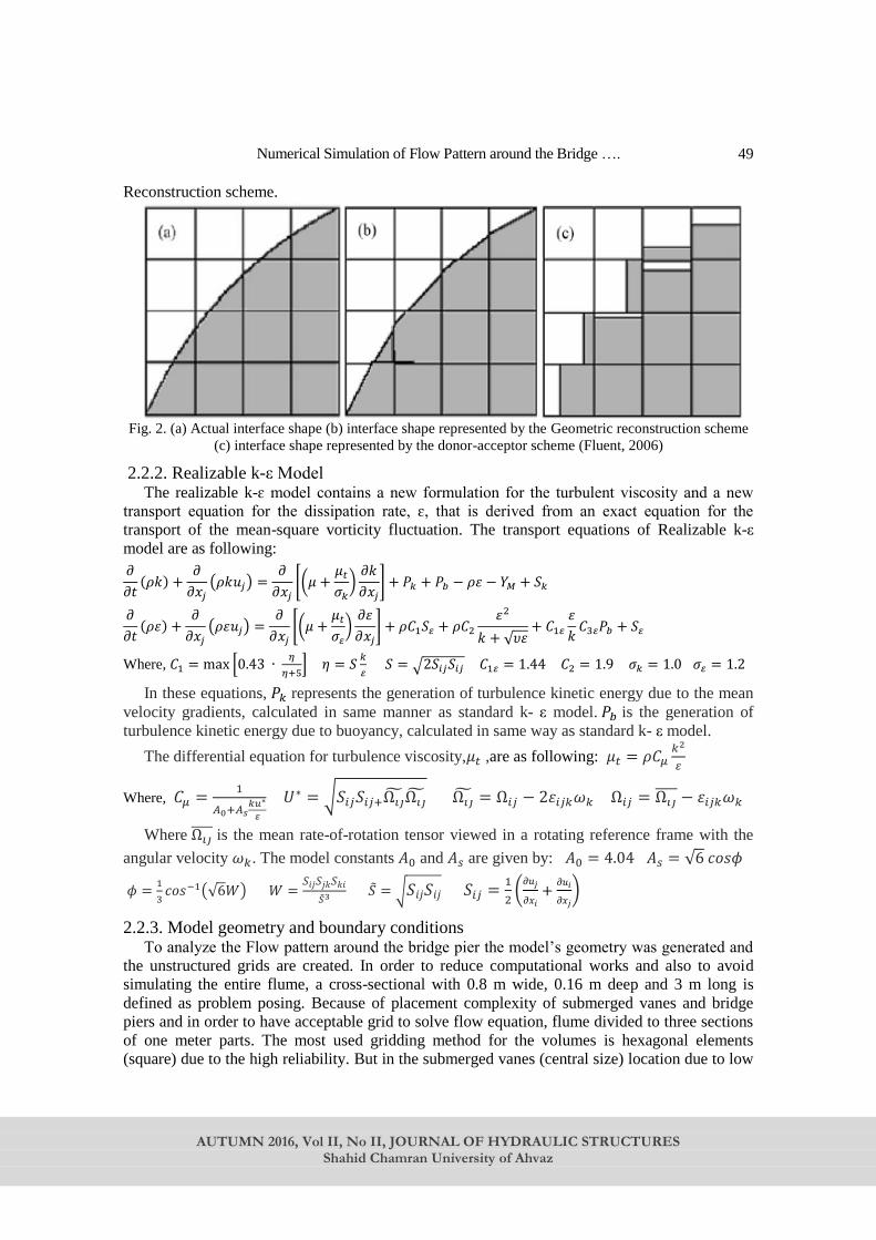
Numerical Simulation of Flow Pattern around the Bridge ….
AUTUMN 2016, Vol II, No II, JOURNAL OF HYDRAULIC STRUCTURES
Shahid Chamran University of Ahvaz
49
Reconstruction scheme.
Fig. 2. (a) Actual interface shape (b) interface shape represented by the Geometric reconstruction scheme
(c) interface shape represented by the donor-acceptor scheme (Fluent, 2006)
2.2.2. Realizable k-ε Model The realizable k-ɛ model contains a new formulation for the turbulent viscosity and a new
transport equation for the dissipation rate, ɛ, that is derived from an exact equation for the
transport of the mean-square vorticity fluctuation. The transport equations of Realizable k-ε
model are as following:
𝜕
𝜕𝑡(𝜌𝑘) +
𝜕
𝜕𝑥𝑗
(𝜌𝑘𝑢𝑗) =𝜕
𝜕𝑥𝑗
[(𝜇 +𝜇𝑡
𝜎𝑘
)𝜕𝑘
𝜕𝑥𝑗
] + 𝑃𝑘 + 𝑃𝑏 − 𝜌𝜀 − 𝑌𝑀 + 𝑆𝑘
𝜕
𝜕𝑡(𝜌𝜀) +
𝜕
𝜕𝑥𝑗
(𝜌𝜀𝑢𝑗) =𝜕
𝜕𝑥𝑗
[(𝜇 +𝜇𝑡
𝜎𝜀
)𝜕𝜀
𝜕𝑥𝑗
] + 𝜌𝐶1𝑆𝜀 + 𝜌𝐶2
𝜀2
𝑘 + √𝜐𝜀+ 𝐶1𝜀
𝜀
𝑘𝐶3𝜀𝑃𝑏 + 𝑆𝜀
Where, 𝐶1 = max [0.43 ∙ 𝜂
𝜂+5] 𝜂 = 𝑆
𝑘
𝜀 𝑆 = √2𝑆𝑖𝑗𝑆𝑖𝑗 𝐶1𝜀 = 1.44 𝐶2 = 1.9 𝜎𝑘 = 1.0 𝜎𝜀 = 1.2
In these equations, 𝑃𝑘 represents the generation of turbulence kinetic energy due to the mean
velocity gradients, calculated in same manner as standard k- ε model. 𝑃𝑏 is the generation of
turbulence kinetic energy due to buoyancy, calculated in same way as standard k- ε model.
The differential equation for turbulence viscosity,𝜇𝑡 ,are as following: 𝜇𝑡 = 𝜌𝐶𝜇𝑘2
𝜀
Where, 𝐶𝜇 =1
𝐴0+𝐴𝑠𝑘𝑢∗
𝜀
𝑈∗ = √𝑆𝑖𝑗𝑆𝑖𝑗+Ω𝑖�̃�Ω𝑖�̃� Ω𝑖�̃� = Ω𝑖𝑗 − 2𝜀𝑖𝑗𝑘𝜔𝑘 Ω𝑖𝑗 = Ω𝑖𝑗̅̅ ̅̅ − 𝜀𝑖𝑗𝑘𝜔𝑘
Where Ω𝑖𝑗̅̅ ̅̅ is the mean rate-of-rotation tensor viewed in a rotating reference frame with the
angular velocity 𝜔𝑘. The model constants 𝐴0 and 𝐴𝑠 are given by: 𝐴0 = 4.04 𝐴𝑠 = √6 𝑐𝑜𝑠𝜙
𝜙 =1
3𝑐𝑜𝑠−1(√6𝑊) 𝑊 =
𝑆𝑖𝑗𝑆𝑗𝑘𝑆𝑘𝑖
�̃�3 �̃� = √𝑆𝑖𝑗𝑆𝑖𝑗 𝑆𝑖𝑗 =1
2(
𝜕𝑢𝑗
𝜕𝑥𝑖+
𝜕𝑢𝑖
𝜕𝑥𝑗)
2.2.3. Model geometry and boundary conditions To analyze the Flow pattern around the bridge pier the model’s geometry was generated and
the unstructured grids are created. In order to reduce computational works and also to avoid
simulating the entire flume, a cross-sectional with 0.8 m wide, 0.16 m deep and 3 m long is
defined as problem posing. Because of placement complexity of submerged vanes and bridge
piers and in order to have acceptable grid to solve flow equation, flume divided to three sections
of one meter parts. The most used gridding method for the volumes is hexagonal elements
(square) due to the high reliability. But in the submerged vanes (central size) location due to low

S. Haji Azizi, D. Farsadizadeh, H. Arvanaghi, A. Abbaspour
AUTUMN 2016, Vol II, No II, JOURNAL OF HYDRAULIC STRUCTURES
Shahid Chamran University of Ahvaz
50
thickness of the vanes (1 mm) the tetrahedron (triangular) elements was used. In order to make
acceptable mesh in the pier area the Quad-Pave algorithms and in other parts the Quad-Map
algorithm was used. Meshing volumes in the pier area with algorithms Hex-Cooper and in other
parts of the Hex-Map algorithm was performed. In the final step, the boundary conditions for
walls, pier and submerged vanes, input and output page and also velocity inlet defined and saved
by *.msh format in order to import it to Fluent software. One of the constructed mesh files in
Gambit presented as Fig. 3.
Fig. 3. Grid for pier area and four submerged vanes
3. Results and Discussions
3.1. Calibration of the numerical model In order to calibrate a numerical model, the experimental results of Arvanaqhi (2009) is used.
His experiments in rectangular channel with a length of 10 meters, width of 0.25 m and a height
of 0.50 m was peformed. Diameter of the model pier used in this series of experiments was
0.012 m. In order to calibrate the numerical model, depth and velocity parameters (profiles of
water level and flow velocity profiles), experimental and numerical models compared. In
experimental models, the water depth measured by bathymetry sensors at the top of the channel
and upstream of the bridge pier, and it was controlled and corrected using gauge surface. as well
as, the horizontal component of the flow velocity (Vx) around bridge pier, extracted by Micro
Propeller in two model V/Vc within accuracy of 1.0 centimeters per second. In order to calibrate,
the velocity distribution profile, along the longitudinal axis of channel (Z = 0) and in two
sections by distance 3 and 10 cm from the center of the bridge piers in the upstream and in V /
Vc = 0.95 was investigated. Also, the water surface profile on two axes Z = 0 (central axis) and Z
= ± 3 cm (lateral axis) was extracted and compared to experimental results.
Initially to choose the best model of turbulence, k-ε turbulence model using three models of
Standard, RNG and Realizable investigated and the results of numerical models compared to
experimental results and Relative Average Error (RAE) was calculated. In the following
equation (𝑣𝑝) and (𝑣𝑛) respectively, are flow velocity in the physical models and the Numerical
models.
(𝑅𝐴𝐸)𝑉% =∑ |(𝑣𝑝𝑖 − 𝑣𝑛𝑖)|𝑁
𝑖=1
∑ 𝑣𝑝𝑖𝑁𝑖=1
× 100
According to Figure 4 and Table 2, comparison of the results showed that Realizable
turbulence model is much in tune with experimental results. It seems that because of the low
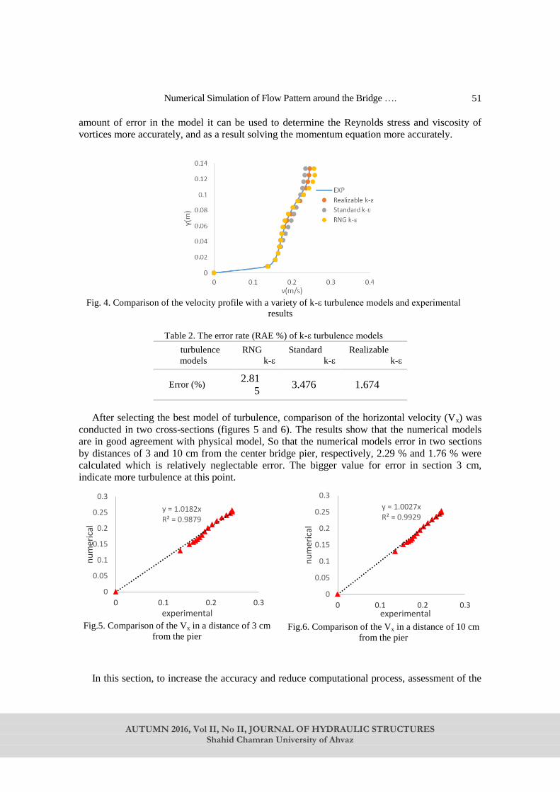
Numerical Simulation of Flow Pattern around the Bridge ….
AUTUMN 2016, Vol II, No II, JOURNAL OF HYDRAULIC STRUCTURES
Shahid Chamran University of Ahvaz
51
amount of error in the model it can be used to determine the Reynolds stress and viscosity of
vortices more accurately, and as a result solving the momentum equation more accurately.
Fig. 4. Comparison of the velocity profile with a variety of k-ε turbulence models and experimental
results
Table 2. The error rate (RAE %) of k-ε turbulence models Realizable
k-ε Standard
k-ε RNG
k-ε turbulence
models
1.674 3.476 2.81
5 Error (%)
After selecting the best model of turbulence, comparison of the horizontal velocity (Vx) was
conducted in two cross-sections (figures 5 and 6). The results show that the numerical models
are in good agreement with physical model, So that the numerical models error in two sections
by distances of 3 and 10 cm from the center bridge pier, respectively, 2.29 % and 1.76 % were
calculated which is relatively neglectable error. The bigger value for error in section 3 cm,
indicate more turbulence at this point.
Fig.5. Comparison of the Vx in a distance of 3 cm
from the pier Fig.6. Comparison of the Vx in a distance of 10 cm
from the pier
In this section, to increase the accuracy and reduce computational process, assessment of the
y = 1.0182x R² = 0.9879
0
0.05
0.1
0.15
0.2
0.25
0.3
0 0.1 0.2 0.3
nu
mer
ical
experimental
y = 1.0027x R² = 0.9929
0
0.05
0.1
0.15
0.2
0.25
0.3
0 0.1 0.2 0.3
nu
mer
ical
experimental
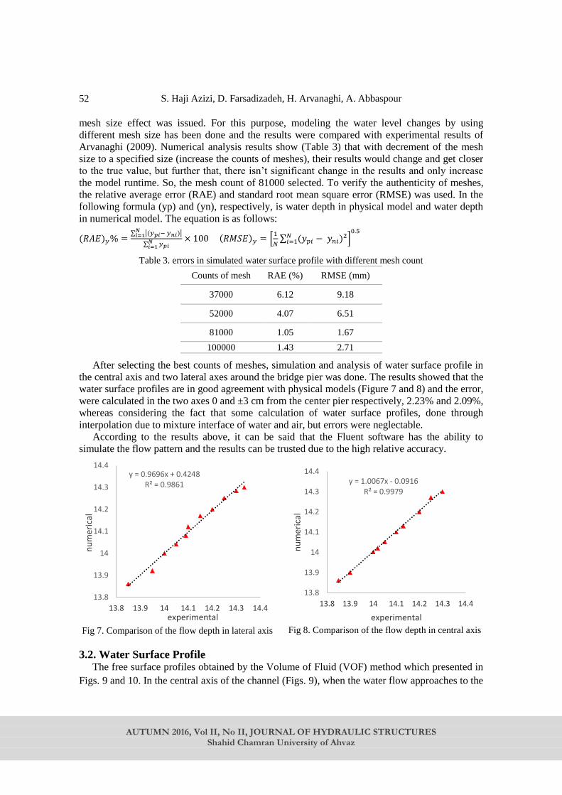
S. Haji Azizi, D. Farsadizadeh, H. Arvanaghi, A. Abbaspour
AUTUMN 2016, Vol II, No II, JOURNAL OF HYDRAULIC STRUCTURES
Shahid Chamran University of Ahvaz
52
mesh size effect was issued. For this purpose, modeling the water level changes by using
different mesh size has been done and the results were compared with experimental results of
Arvanaghi (2009). Numerical analysis results show (Table 3) that with decrement of the mesh
size to a specified size (increase the counts of meshes), their results would change and get closer
to the true value, but further that, there isn’t significant change in the results and only increase
the model runtime. So, the mesh count of 81000 selected. To verify the authenticity of meshes,
the relative average error (RAE) and standard root mean square error (RMSE) was used. In the
following formula (yp) and (yn), respectively, is water depth in physical model and water depth
in numerical model. The equation is as follows:
(𝑅𝐴𝐸)𝑦% =∑ |(𝑦𝑝𝑖− 𝑦𝑛𝑖)|𝑁
𝑖=1
∑ 𝑦𝑝𝑖𝑁𝑖=1
× 100 (𝑅𝑀𝑆𝐸)𝑦 = [1
𝑁∑ (𝑦𝑝𝑖 − 𝑦𝑛𝑖)2𝑁
𝑖=1 ]0.5
Table 3. errors in simulated water surface profile with different mesh count
RMSE (mm) RAE (%) Counts of mesh
9.18 6.12 37000
6.51 4.07 52000
1.67 1.05 81000
2.71 1.43 100000
After selecting the best counts of meshes, simulation and analysis of water surface profile in
the central axis and two lateral axes around the bridge pier was done. The results showed that the
water surface profiles are in good agreement with physical models (Figure 7 and 8) and the error,
were calculated in the two axes 0 and ±3 cm from the center pier respectively, 2.23% and 2.09%,
whereas considering the fact that some calculation of water surface profiles, done through
interpolation due to mixture interface of water and air, but errors were neglectable.
According to the results above, it can be said that the Fluent software has the ability to
simulate the flow pattern and the results can be trusted due to the high relative accuracy.
Fig 7. Comparison of the flow depth in lateral axis
Fig 8. Comparison of the flow depth in central axis
3.2. Water Surface Profile The free surface profiles obtained by the Volume of Fluid (VOF) method which presented in
Figs. 9 and 10. In the central axis of the channel (Figs. 9), when the water flow approaches to the
y = 0.9696x + 0.4248 R² = 0.9861
13.8
13.9
14
14.1
14.2
14.3
14.4
13.8 13.9 14 14.1 14.2 14.3 14.4
nu
mer
ical
experimental
y = 1.0067x - 0.0916 R² = 0.9979
13.8
13.9
14
14.1
14.2
14.3
14.4
13.8 13.9 14 14.1 14.2 14.3 14.4
nu
mer
ical
experimental
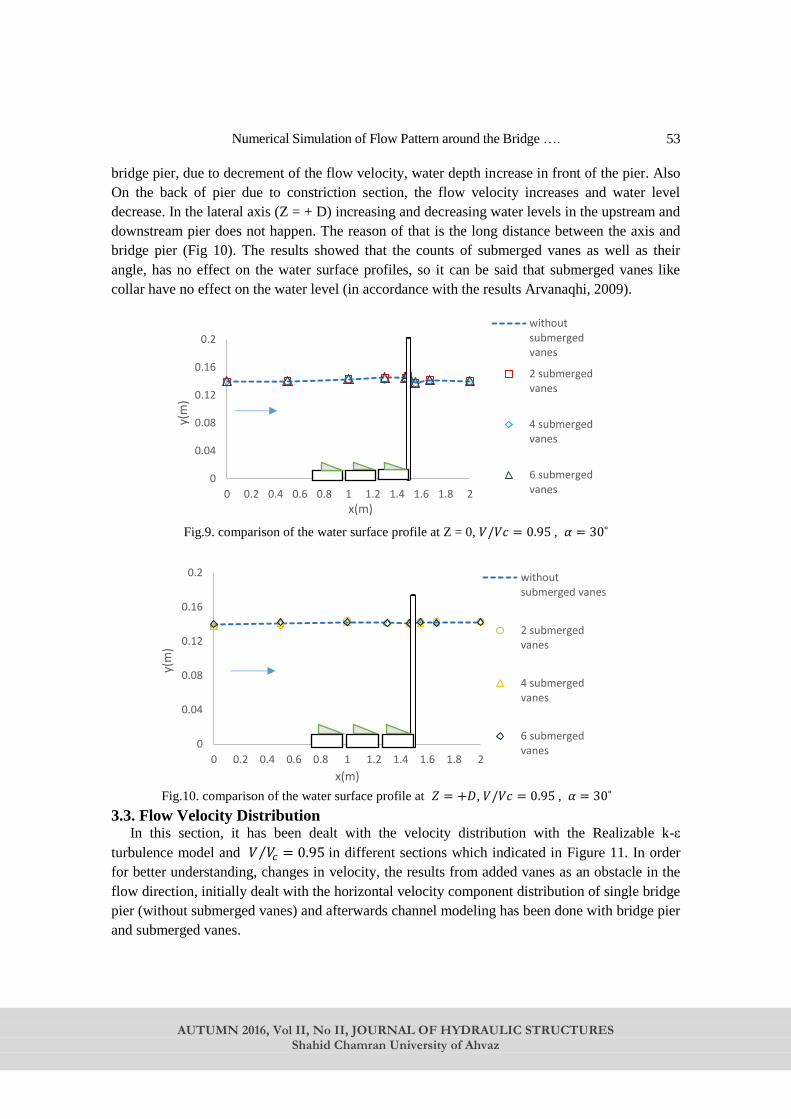
Numerical Simulation of Flow Pattern around the Bridge ….
AUTUMN 2016, Vol II, No II, JOURNAL OF HYDRAULIC STRUCTURES
Shahid Chamran University of Ahvaz
53
bridge pier, due to decrement of the flow velocity, water depth increase in front of the pier. Also
On the back of pier due to constriction section, the flow velocity increases and water level
decrease. In the lateral axis (Z = + D) increasing and decreasing water levels in the upstream and
downstream pier does not happen. The reason of that is the long distance between the axis and
bridge pier (Fig 10). The results showed that the counts of submerged vanes as well as their
angle, has no effect on the water surface profiles, so it can be said that submerged vanes like
collar have no effect on the water level (in accordance with the results Arvanaqhi, 2009).
Fig.9. comparison of the water surface profile at Z = 0, 𝑉/𝑉𝑐 = 0.95 , 𝛼 = 30˚
Fig.10. comparison of the water surface profile at 𝑍 = +𝐷, 𝑉/𝑉𝑐 = 0.95 , 𝛼 = 30˚
3.3. Flow Velocity Distribution In this section, it has been dealt with the velocity distribution with the Realizable k-ε
turbulence model and 𝑉 𝑉𝑐⁄ = 0.95 in different sections which indicated in Figure 11. In order
for better understanding, changes in velocity, the results from added vanes as an obstacle in the
flow direction, initially dealt with the horizontal velocity component distribution of single bridge
pier (without submerged vanes) and afterwards channel modeling has been done with bridge pier
and submerged vanes.
0
0.04
0.08
0.12
0.16
0.2
0 0.2 0.4 0.6 0.8 1 1.2 1.4 1.6 1.8 2
y(m
)
x(m)
withoutsubmergedvanes
2 submergedvanes
4 submergedvanes
6 submergedvanes
0
0.04
0.08
0.12
0.16
0.2
0 0.2 0.4 0.6 0.8 1 1.2 1.4 1.6 1.8 2
y(m
)
x(m)
withoutsubmerged vanes
2 submergedvanes
4 submergedvanes
6 submergedvanes
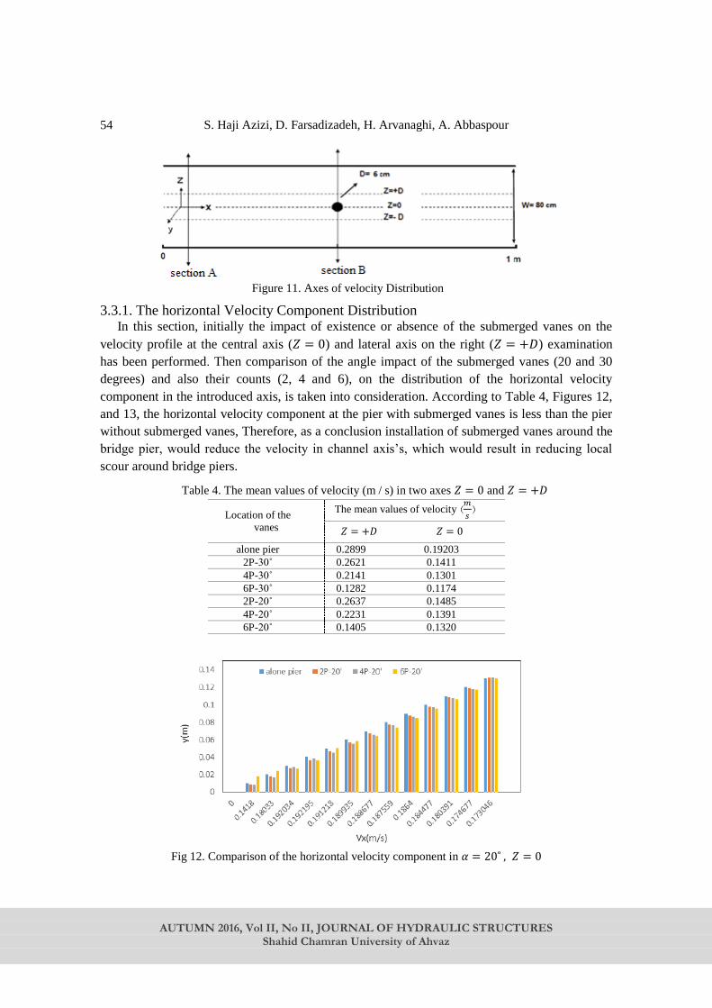
S. Haji Azizi, D. Farsadizadeh, H. Arvanaghi, A. Abbaspour
AUTUMN 2016, Vol II, No II, JOURNAL OF HYDRAULIC STRUCTURES
Shahid Chamran University of Ahvaz
54
Figure 11. Axes of velocity Distribution
3.3.1. The horizontal Velocity Component Distribution In this section, initially the impact of existence or absence of the submerged vanes on the
velocity profile at the central axis (𝑍 = 0) and lateral axis on the right (𝑍 = +𝐷) examination
has been performed. Then comparison of the angle impact of the submerged vanes (20 and 30
degrees) and also their counts (2, 4 and 6), on the distribution of the horizontal velocity
component in the introduced axis, is taken into consideration. According to Table 4, Figures 12,
and 13, the horizontal velocity component at the pier with submerged vanes is less than the pier
without submerged vanes, Therefore, as a conclusion installation of submerged vanes around the
bridge pier, would reduce the velocity in channel axis’s, which would result in reducing local
scour around bridge piers.
Table 4. The mean values of velocity (m / s) in two axes 𝑍 = 0 and 𝑍 = +𝐷
(𝑚
𝑠 )The mean values of velocity
Location of the
vanes 𝑍 = 0 𝑍 = +𝐷 0.19203 0.2899 alone pier
0.1411 0.2621 2P-30˚
0.1301 0.2141 4P-30˚ 0.1174 0.1282 6P-30˚ 0.1485 0.2637 2P-20˚ 0.1391 0.2231 4P-20˚ 0.1320 0.1405 6P-20˚
Fig 12. Comparison of the horizontal velocity component in 𝛼 = 20˚ , 𝑍 = 0
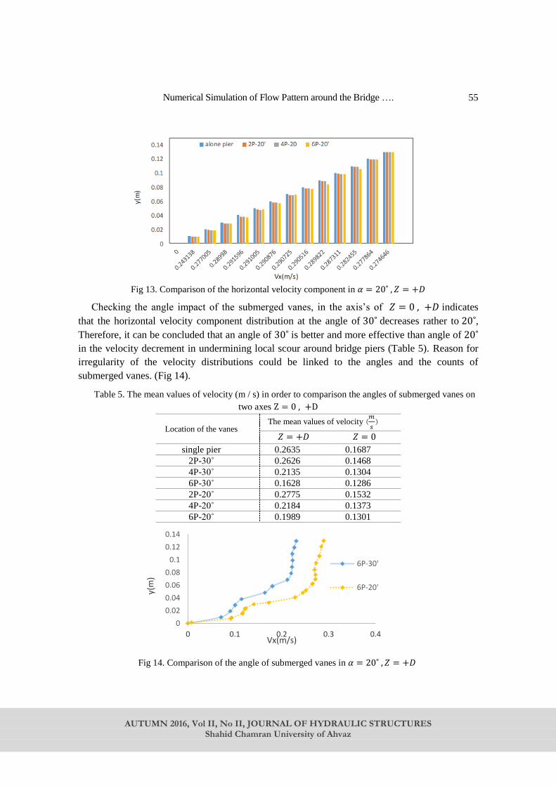
Numerical Simulation of Flow Pattern around the Bridge ….
AUTUMN 2016, Vol II, No II, JOURNAL OF HYDRAULIC STRUCTURES
Shahid Chamran University of Ahvaz
55
Fig 13. Comparison of the horizontal velocity component in 𝛼 = 20˚ , 𝑍 = +𝐷
Checking the angle impact of the submerged vanes, in the axis’s of 𝑍 = 0 , +𝐷 indicates
that the horizontal velocity component distribution at the angle of 30˚ decreases rather to 20˚,
Therefore, it can be concluded that an angle of 30˚ is better and more effective than angle of 20˚
in the velocity decrement in undermining local scour around bridge piers (Table 5). Reason for
irregularity of the velocity distributions could be linked to the angles and the counts of
submerged vanes. (Fig 14).
Table 5. The mean values of velocity (m / s) in order to comparison the angles of submerged vanes on
two axes Z = 0 , +D
(𝑚
𝑠 )The mean values of velocity
Location of the vanes 𝑍 = 0 𝑍 = +𝐷
0.1687 0.2635 single pier
0.1468 0.2626 2P-30˚
0.1304 0.2135 4P-30˚
0.1286 0.1628 6P-30˚
0.1532 0.2775 2P-20˚
0.1373 0.2184 4P-20˚
0.1301 0.1989 6P-20˚
Fig 14. Comparison of the angle of submerged vanes in 𝛼 = 20˚ , 𝑍 = +𝐷
0
0.02
0.04
0.06
0.08
0.1
0.12
0.14
0 0.1 0.2 0.3 0.4
y(m
)
Vx(m/s)
6P-30'
6P-20'
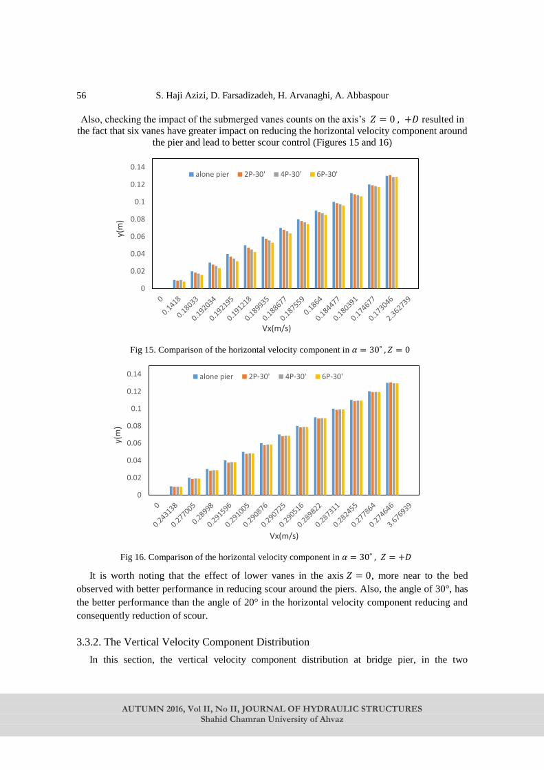
S. Haji Azizi, D. Farsadizadeh, H. Arvanaghi, A. Abbaspour
AUTUMN 2016, Vol II, No II, JOURNAL OF HYDRAULIC STRUCTURES
Shahid Chamran University of Ahvaz
56
Also, checking the impact of the submerged vanes counts on the axis’s 𝑍 = 0 , +𝐷 resulted in
the fact that six vanes have greater impact on reducing the horizontal velocity component around
the pier and lead to better scour control (Figures 15 and 16)
Fig 15. Comparison of the horizontal velocity component in 𝛼 = 30˚ , 𝑍 = 0
Fig 16. Comparison of the horizontal velocity component in 𝛼 = 30˚ , 𝑍 = +𝐷
It is worth noting that the effect of lower vanes in the axis 𝑍 = 0, more near to the bed
observed with better performance in reducing scour around the piers. Also, the angle of 30°, has
the better performance than the angle of 20° in the horizontal velocity component reducing and
consequently reduction of scour.
3.3.2. The Vertical Velocity Component Distribution
In this section, the vertical velocity component distribution at bridge pier, in the two
0
0.02
0.04
0.06
0.08
0.1
0.12
0.14
y(m
)
Vx(m/s)
alone pier 2P-30' 4P-30' 6P-30'
0
0.02
0.04
0.06
0.08
0.1
0.12
0.14
y(m
)
Vx(m/s)
alone pier 2P-30' 4P-30' 6P-30'
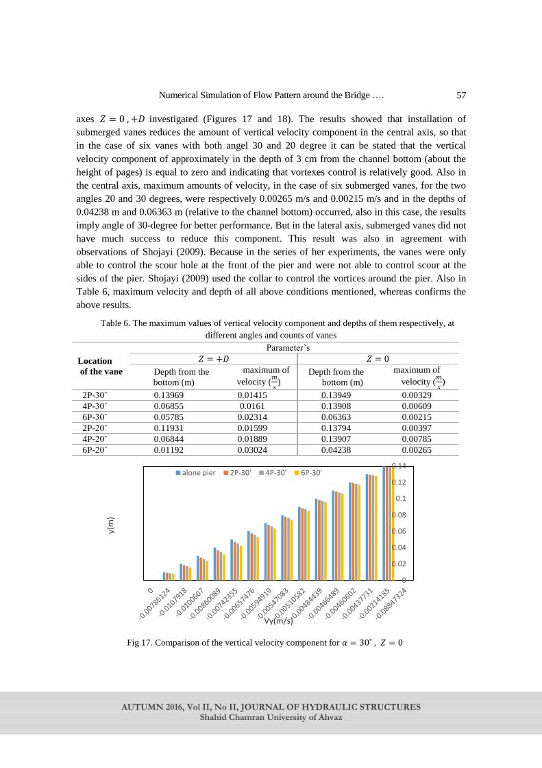
Numerical Simulation of Flow Pattern around the Bridge ….
AUTUMN 2016, Vol II, No II, JOURNAL OF HYDRAULIC STRUCTURES
Shahid Chamran University of Ahvaz
57
axes 𝑍 = 0 , +𝐷 investigated (Figures 17 and 18). The results showed that installation of
submerged vanes reduces the amount of vertical velocity component in the central axis, so that
in the case of six vanes with both angel 30 and 20 degree it can be stated that the vertical
velocity component of approximately in the depth of 3 cm from the channel bottom (about the
height of pages) is equal to zero and indicating that vortexes control is relatively good. Also in
the central axis, maximum amounts of velocity, in the case of six submerged vanes, for the two
angles 20 and 30 degrees, were respectively 0.00265 m/s and 0.00215 m/s and in the depths of
0.04238 m and 0.06363 m (relative to the channel bottom) occurred, also in this case, the results
imply angle of 30-degree for better performance. But in the lateral axis, submerged vanes did not
have much success to reduce this component. This result was also in agreement with
observations of Shojayi (2009). Because in the series of her experiments, the vanes were only
able to control the scour hole at the front of the pier and were not able to control scour at the
sides of the pier. Shojayi (2009) used the collar to control the vortices around the pier. Also in
Table 6, maximum velocity and depth of all above conditions mentioned, whereas confirms the
above results.
Table 6. The maximum values of vertical velocity component and depths of them respectively, at
different angles and counts of vanes
Parameter’s
Location
of the vane
𝑍 = 0 𝑍 = +𝐷
maximum of
velocity (𝑚
𝑠)
Depth from the
bottom (m)
maximum of
velocity (𝑚
𝑠)
Depth from the
bottom (m)
0.00329 0.13949 0.01415 0.13969 2P-30˚
0.00609 0.13908 0.0161 0.06855 4P-30˚
0.00215 0.06363 0.02314 0.05785 6P-30˚
0.00397 0.13794 0.01599 0.11931 2P-20˚
0.00785 0.13907 0.01889 0.06844 4P-20˚
0.00265 0.04238 0.03024 0.01192 6P-20˚
Fig 17. Comparison of the vertical velocity component for 𝛼 = 30˚ , 𝑍 = 0
0
0.02
0.04
0.06
0.08
0.1
0.12
0.14
y(m
)
Vy(m/s)
alone pier 2P-30' 4P-30' 6P-30'
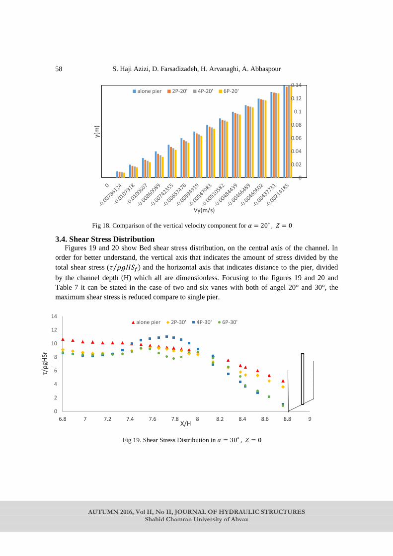
S. Haji Azizi, D. Farsadizadeh, H. Arvanaghi, A. Abbaspour
AUTUMN 2016, Vol II, No II, JOURNAL OF HYDRAULIC STRUCTURES
Shahid Chamran University of Ahvaz
58
Fig 18. Comparison of the vertical velocity component for 𝛼 = 20˚ , 𝑍 = 0
3.4. Shear Stress Distribution Figures 19 and 20 show Bed shear stress distribution, on the central axis of the channel. In
order for better understand, the vertical axis that indicates the amount of stress divided by the
total shear stress (𝜏 𝜌𝑔𝐻𝑆𝑓)⁄ and the horizontal axis that indicates distance to the pier, divided
by the channel depth (H) which all are dimensionless. Focusing to the figures 19 and 20 and
Table 7 it can be stated in the case of two and six vanes with both of angel 20° and 30°, the
maximum shear stress is reduced compare to single pier.
Fig 19. Shear Stress Distribution in 𝛼 = 30˚ , 𝑍 = 0
0
0.02
0.04
0.06
0.08
0.1
0.12
0.14
y(m
)
Vy(m/s)
alone pier 2P-20' 4P-20' 6P-20'
0
2
4
6
8
10
12
14
6.8 7 7.2 7.4 7.6 7.8 8 8.2 8.4 8.6 8.8 9
τ/ρgH
Sf
X/H
alone pier 2P-30' 4P-30' 6P-30'
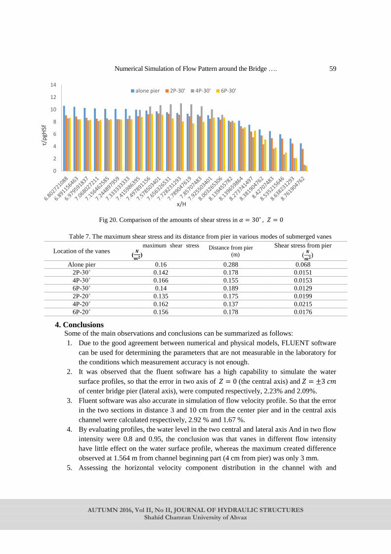
Numerical Simulation of Flow Pattern around the Bridge ….
AUTUMN 2016, Vol II, No II, JOURNAL OF HYDRAULIC STRUCTURES
Shahid Chamran University of Ahvaz
59
Fig 20. Comparison of the amounts of shear stress in 𝛼 = 30˚ , 𝑍 = 0
Table 7. The maximum shear stress and its distance from pier in various modes of submerged vanes Shear stress from pier
(𝑵
𝒎𝟐) Distance from pier
(m)
maximum shear stress
(𝑵
𝒎𝟐) Location of the vanes
0.068 0.288 0.16 Alone pier
0.0151 0.178 0.142 2P-30˚
0.0153 0.155 0.166 4P-30˚
0.0129 0.189 0.14 6P-30˚
0.0199 0.175 0.135 2P-20˚
0.0215 0.137 0.162 4P-20˚
0.0176 0.178 0.156 6P-20˚
4. Conclusions Some of the main observations and conclusions can be summarized as follows:
1. Due to the good agreement between numerical and physical models, FLUENT software
can be used for determining the parameters that are not measurable in the laboratory for
the conditions which measurement accuracy is not enough.
2. It was observed that the fluent software has a high capability to simulate the water
surface profiles, so that the error in two axis of 𝑍 = 0 (the central axis) and 𝑍 = ±3 𝑐𝑚
of center bridge pier (lateral axis), were computed respectively, 2.23% and 2.09%.
3. Fluent software was also accurate in simulation of flow velocity profile. So that the error
in the two sections in distance 3 and 10 cm from the center pier and in the central axis
channel were calculated respectively, 2.92 % and 1.67 %.
4. By evaluating profiles, the water level in the two central and lateral axis And in two flow
intensity were 0.8 and 0.95, the conclusion was that vanes in different flow intensity
have little effect on the water surface profile, whereas the maximum created difference
observed at 1.564 m from channel beginning part (4 cm from pier) was only 3 mm.
5. Assessing the horizontal velocity component distribution in the channel with and
0
2
4
6
8
10
12
14
τ/ρgH
Sf
x/H
alone pier 2P-30' 4P-30' 6P-30'
S. Haji Azizi, D. Farsadizadeh, H. Arvanaghi, A. Abbaspour
AUTUMN 2016, Vol II, No II, JOURNAL OF HYDRAULIC STRUCTURES
Shahid Chamran University of Ahvaz
60
without the bridge pier and submerged vanes, it was observed that the horizontal
velocity component reduced using submerged vanes and it means that the vanes are
effective in reduction of velocity and subsequently reduction of local scour around
bridge piers.
6. Evaluating and comparing the angle of the submerged vanes on central and lateral axis’s
in the channel it was observed that the angle of 30° is better than the angle 20 ° in
reduction of horizontal velocity component.
7. Considering the counts of used submerged vanes, it turned out that the counts of 6 was
much effective rather than 2 and 4 in reducing of the horizontal velocity component.
8. The studies showed the efficiency of vanes in velocity decrement near to the channel
bed, whereas implies on positive performance of submerged vanes.
9. Assessing the vertical velocity component in the central axis resulted in the fact that in
general, existence of vanes reduces this component. So that, placement of six vanes with
both angels of 20 and 30 degree in the central axis, the vertical velocity component was
approximately equal to zero in 3 cm of the channel bottom (the same height of vanes).
References 1. Fluent 6.3 User’s Guide. (2006). Fluent Incorporated, Lebanon, N.H.
2. Ariyan far, e., and shafaei bajestan, m. (2008). “Numerical Study the flow pattern around the
cylindrical bridge piers by fluent”. The Fourth National Congress of Civil Engineering,
Tehran, Tehran University.
3. Arvanaghi, h. (2009). “Study the Reduction of Scour the around of bridge piers with
rectangular collar by experimental method and by used simulate the flow pattern around it
with turbulence models”, PhD Thesis, Department of Water Engineering University of
Tabriz.
4. Asadi partov, a., eghbal zadeh, a., and ahmadi, a. (2012). “The study effect of bridge piers
diameter, on the flow pattern in the direct channel by using Flow-3D software” Eleventh
Iranian Hydraulic Conference, 16 to 18 November, Urmia University.
5. Besharati givi, m., and hakim zadeh, h. (2009). “Numerical Study of flow pattern and shear
stress around the tapered piers”. Journal of Marine Engineering, Volume VI, Issue 11.
6. Marelius, F. and Sinha, S.K., (1998), “Experimental investigation of flow past submerged
vanes”, J. Hyd. Eng., ASCE, 124(5): 542-545.
7. Roulund, A., Sumer, B.M., Fredsoe, J. and Michelsen, J., 2002, 3D Numerical Modeling of
Flow and Scour around a Pile, Proceeding First International Conference on Scour of
Foundations, Texas A & M University, Texas, USA: 795-809.
8. Yen, C.L., Lai, J.S. and Chang, W.Y., 2001, Modeling 3D flow and scouring around circular
piers, Proc.Nati.Sci.Counc.ROC (A), 25(1): 17-26.
9. Hasan zadeh, Y., hakim zadeh, h., norani, v., and sarveram, h. (2006), “a numerical model to
simulate the flow pattern around bridge piers”, Seventh International Seminar of river
engineering, Faculty of Science and Engineering water, shahid Chamran University.
10. Sarveram, h., hasan zade, Y., and hakim zadeh, h. (2008). “Study Flow velocity distribution
at bridge pier by using numerical models”, the eighth International Congress of Civil
Engineering, Shiraz University.
11. Shojayi, p. (2009). “Combined effects of vanes and a collar, in reducing Scour of the
cylindrical bridges pier”, Master Thesis, Department of Water Engineering University of

Numerical Simulation of Flow Pattern around the Bridge ….
AUTUMN 2016, Vol II, No II, JOURNAL OF HYDRAULIC STRUCTURES
Shahid Chamran University of Ahvaz
61
Tabriz.
12. Alamayiyan, a., and jafar zadeh, m.r.(2009). “Numerical study of flow conditions in a
collision with bridge pier”, thr Eighth International Seminar of river engineering, shahid
Chamran University.
13. Karimi nia, a., and salehi neyshabori, a.a. (2011). “Numerical simulation of phenomenon of
back water at the bridge’s pier, Journal of Civil Engineering and mapping, Technical Faculty
of Tehran University, Volume 45, Issue 4, Pages 493-487.
14. Kolali, f., ghodsiyan, m., and rostam abadi, m. (2012), “Numerical simulation of the flow
pattern around bridge slant piers, in plane perpendicular to the flow to the right and left” , the
ninth international seminar of river engineering, shahid Chamran University.
15. Hoshmand, d.a., esmaeili, k., keshavarzi, a., and farid hoseini, a. (2013), “Numerical
modeling of flow around the bridge pier in meandering beds”, Journal of Soil and Water,
Ferdowsi University of Mashhad, Vol. 27, No. 5: 984-973.
AUTUMN 2016, Vol II, No II, JOURNAL OF HYDRAULIC STRUCTURES
Shahid Chamran University of Ahvaz
Journal of Hydraulic Structures
J. Hydraul. Struct., 2016; 2(2):62-73
DOI: 10.22055/jhs.2016.12853
Flood Forecasting Using Artificial Neural Networks: an
Application of Multi-Model Data Fusion Technique
Yaser Tahmasebi Biragani1,2
Farhad Yazdandoost3
Hossein Ghalkhani4
Abstract Floods are among the natural disasters that cause human hardship and economic loss.
Establishing a viable flood forecasting and warning system for communities at risk can mitigate
these adverse effects. However, establishing an accurate flood forecasting system is still
challenging due to the lack of knowledge about the effective variables in forecasting. The
present study has indicated that the use of artificial intelligence, especially neural networks is
suitable for flood forecasting systems (FFSs). In this research, mathematical modeling of flood
forecasting with the application of Artificial Neural Networks (ANN) and data fusion technique
were used in estimating the flood discharge. Sensitivity analysis was performed to investigate
the significance of each model input and the best MLP ANN architecture. The data used in
developing the model comprise discharge at different time steps, precipitation and antecedent
precipitation index for a major river basin. Application of model on a case study (Karun River in
Iran) indicated that rainfall-runoff process using data fusion approach produces results with
higher degrees of precision.
Keywords: Flood Forecasting, Neural Networks, Data Fusion, Sensitivity Analysis, Karun River
Received: 05 June 2016; Accepted: 23 October 2016
1. Introduction Flood protection and awareness have continued to rise on the political agenda over the last
decade accompanied by a drive to ‘improve’ flood forecasts (Demeritt, et al. [5]; van Berkom,
[12]). Without a doubt, flood flow information is very important for early warning. Flood flows
in downstream areas are strongly influenced by upstream conditions. The artificial neural
network (ANN) model has shown to be appropriate for the above-mentioned problem (Chen et
1
Department of Environmental Health Engineering, School of public Health, Ahvaz Jundishapur
University of Medical Sciences, Ahvaz, Iran, (Corresponding author) 2
Environmental Technologies Research Center (ETRC), Ahvaz Jundishapur University of Medical
Sciences, Ahvaz, Iran
3 Department of Civil Engineering, K. N. Toosi University of Technology, Tehran, Iran
4 Department Water Resources Researches, Water Research Institute, Tehran, Iran
Flood Forecasting Using Artificial Neural Networks ….
AUTUMN 2016, Vol II, No II, JOURNAL OF HYDRAULIC STRUCTURES
Shahid Chamran University of Ahvaz
63
al. [3]). Neural network models possess a distributive processing system and are able to store
inherent characteristics of data in the form of a large storage for later generalization (French et
al. [7]). The ANN model has various mathematical compositions capable of modeling extremely
complex physical systems. It has the potential to be more flexible and less assumption dependent
approach to act as a simulation model for the hydrologic systems (Sudheer and Jain [11]). In this
paper, a model has been presented for flood forecasting using data fusion technique and artificial
neural networks (ANNs). Data fusion is an emerging area of research that covers a broad
spectrum of application areas ranging from ocean surveillance to strategic warning, and medical
diagnosis (Hall [8]). The principal objective of data fusion, which is process of combining or
amalgamating information from multiple sensors and/or data sources, is to provide a solution
that is either more accurate according to some measure of evaluation, or allows one to make
additional inferences above and beyond those that could be achieved through the use of single
source data alone (Dasarathy [4]). Data fusion researches are divided into two board groups. The
first takes the view that data fusion is the amalgamation of raw information to produce an output,
while the second advocate a more generalized view of data fusion in which both raw and
processed information can be fused into useful outputs including higher level decision. See and
Abrahart used data fusion approach for continuous river level forecasting where data was the
amalgamation of information from multiple sensors and different data sources (See and Abrahart
[9]). Abrahart and See evaluated six data fusion strategies and found that data fusion by an
(ANN) model provided the best solution (Abart and See [1]). Shu and Burn applied (ANN)
ensembles in pooled flood frequency analysis for estimating the index flood and the 10-year
flood quintiles (Shu and Burn [10]). Araghinejad et al. [2] applied the combination of data fusion
technique and probabilistic method to forecast peak discharge of Red River in Canada and
seasonal stream flow in Zayandeh-rud River in Iran. Despite remarkable studies in this field,
further investigations need to be conducted to find the effects of various inputs in forecasting
models. This study considers several combination of the different-input models. These inputs
range from discharge at different time steps to precipitation and antecedent precipitation index
(API).
The remainder of the paper is organized in the following sections: section 2 is associated with
the methodology of the study. The methodology section explains data fusion method, typical
ANN model as well as different-input ANN models. In section 3, proposed methodology is
applied on Karun River in Iran as a case study. Combination of the different ANN model with
various inputs are tested on this case study. In the last section, this paper finally gives a
conclusion according detailed results.
2. Methodology
2.1. Data Fusion Methods The general equation of a hydrological event forecasting model is
𝑦𝑖=𝑓(𝑋𝑖) + 𝜀𝑖 𝑖 = 1,2, … 𝑛 (1)
where X= vector of predictors, y= forecast variable, 𝜀 =model error and n= number of
observation data. In the case of using multiple models to forecast y, and considering similar
predictors, Eq. (1) is changed to the following matrix from
[𝑌𝑖] = [
𝑦𝑖1
𝑦𝑖2
⋮𝑦𝑖𝑚
] = [
𝑓1(𝑋𝑖)
𝑓2(𝑋𝑖)⋮
𝑓𝑚(𝑋𝑖)
] + [
𝜀𝑖1
𝜀𝑖2
⋮𝜀𝑖𝑚
] (2)
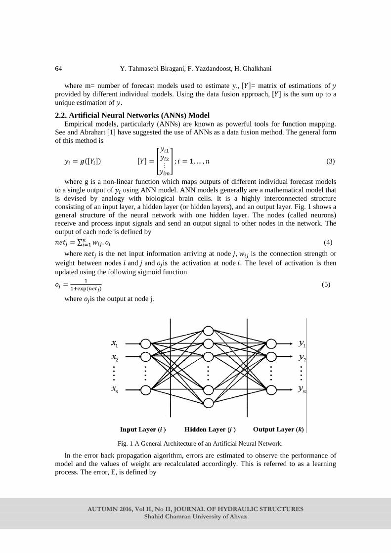
Y. Tahmasebi Biragani, F. Yazdandoost, H. Ghalkhani
AUTUMN 2016, Vol II, No II, JOURNAL OF HYDRAULIC STRUCTURES
Shahid Chamran University of Ahvaz
64
where m= number of forecast models used to estimate y., [𝑌]= matrix of estimations of 𝑦
provided by different individual models. Using the data fusion approach, [𝑌] is the sum up to a
unique estimation of 𝑦.
2.2. Artificial Neural Networks (ANNs) Model Empirical models, particularly (ANNs) are known as powerful tools for function mapping.
See and Abrahart [1] have suggested the use of ANNs as a data fusion method. The general form
of this method is
𝑦𝑖 = 𝑔([𝑌𝑖]) [𝑌] = [
𝑦𝑖1
𝑦𝑖2
⋮𝑦𝑖𝑚
] ; 𝑖 = 1, … , 𝑛 (3)
where g is a non-linear function which maps outputs of different individual forecast models
to a single output of 𝑦𝑖 using ANN model. ANN models generally are a mathematical model that
is devised by analogy with biological brain cells. It is a highly interconnected structure
consisting of an input layer, a hidden layer (or hidden layers), and an output layer. Fig. 1 shows a
general structure of the neural network with one hidden layer. The nodes (called neurons)
receive and process input signals and send an output signal to other nodes in the network. The
output of each node is defined by
𝑛𝑒𝑡𝑗 = ∑ 𝑤𝑖𝑗 . 𝑜𝑖𝑛𝑖=1 (4)
where 𝑛𝑒𝑡𝑗 is the net input information arriving at node 𝑗, 𝑤𝑖𝑗 is the connection strength or
weight between nodes 𝑖 and 𝑗 and 𝑜𝑗is the activation at node 𝑖. The level of activation is then
updated using the following sigmoid function
𝑜𝑗 =1
1+exp (𝑛𝑒𝑡𝑗) (5)
where 𝑜𝑗is the output at node j.
Fig. 1 A General Architecture of an Artificial Neural Network.
In the error back propagation algorithm, errors are estimated to observe the performance of
model and the values of weight are recalculated accordingly. This is referred to as a learning
process. The error, E, is defined by
Flood Forecasting Using Artificial Neural Networks ….
AUTUMN 2016, Vol II, No II, JOURNAL OF HYDRAULIC STRUCTURES
Shahid Chamran University of Ahvaz
65
E=1
2∑ ∑ (𝑑𝑝𝑘 − 𝑜𝑝𝑘)2𝐾
𝑘=1𝑃𝑝=1 (6)
where 𝑃 is the total number of patterns in the training set, 𝐾 is the total number of output
nodes, and 𝑑𝑝𝑘 and 𝑜𝑝𝑘 are the desired and calculated outputs at node 𝑗 for pattern p,
respectively.
A Multi-Layer Perceptron (MLP) method with back propagation is used here which has
input, output, and hidden middle layers.
2.2.1. Model Development One of the main aims in design of warning systems is to increase the pre-warning time based
on accurate simulation of flood inundation levels. Two models were used for this purpose
𝑄(𝑡) = 𝑓[𝑄(𝑡 − 2), 𝑄(𝑡 − 1), 𝑃𝑖(𝑡), 𝑃𝑖(𝑡 − 1), 𝐴𝑃𝐼(𝑋), 𝑇(𝑋), 𝑇(𝑡 − 1)] (7) 𝑄(𝑡 + 1) = 𝑓[𝑄(𝑡 − 1), 𝑄(𝑡), 𝑃𝑖(𝑡), 𝑃𝑖(𝑡 − 1), 𝐴𝑃𝐼(𝑋), 𝑇(𝑡), 𝑇(𝑡 − 1)] (8)
where Q is the discharge, P is the precipitation, T is the temperature and )(xAPI is the
previous precipitation index at previous x time steps and t is the computational time step. The
previous precipitation index may be obtained from:
𝐴𝑃𝐼(𝑋) = ∑ 𝑃𝑋−𝑗. 𝐾−𝑗𝑖𝑗=1 (9)
𝐾 = 𝐸𝑋𝑃(−𝐸𝑇
𝑊𝑚) (10)
where i is the number of passed days, K is the precipitation constant varying between 0.85
and 0.95, jxP is the precipitation at day jx , ET is the evapotranspiration and Wm is the
maximum available soil moisture for evaporation.
2.2.2. Data preprocessing Since input variables appear in different scale, therefore the values of inputs should be
changed in the same scale in a specified interval. Following equations can be used to normalize
input values between (0.05-0.95):
𝑋𝑛 = 0.05 + 0.9𝑋−𝑋𝑚𝑖𝑛
𝑋𝑚𝑎𝑥−𝑋𝑚𝑖𝑛 (11)
where, 𝑋𝑛 is the normalized value of input 𝑋, 𝑋𝑚𝑖𝑛 is the minimum of the input 𝑋 and 𝑋𝑚𝑎𝑥
is the maximum of the input 𝑋.
2.2.3. Evaluating the performance of the model In order to evaluate the performance of ANN models, Nash-sutcliffe, Mean Relative Error
and correlation coefficient parameters are used as following equations:
𝐸 = 1 −∑ (𝑄𝑜𝑏𝑠𝑖−𝑄𝑠𝑖𝑚𝑖)2𝑛
𝑖=1
∑ (𝑄𝑜𝑏𝑠𝑖−�̅�𝑜𝑏𝑠)2𝑛𝑖=1
(12)
𝑀𝑅𝐸 =∑ |
𝑄𝑜𝑏𝑠𝑖−𝑄𝑠𝑖𝑚𝑖𝑄𝑜𝑏𝑠𝑖
|𝑛𝑖=1
𝑛 (13)
𝑅 =𝑛 ∑ (𝑄𝑜𝑏𝑠𝑖.𝑄𝑠𝑖𝑚𝑖)𝑛
𝑖=1 −(∑ 𝑄𝑜𝑏𝑠𝑖𝑛𝑖=1 ).(∑ 𝑄𝑠𝑖𝑚𝑖
𝑛𝑖=1 )
√[𝑛.(∑ 𝑄𝑜𝑏𝑠𝑖2𝑛
𝑖=1 )−(∑ 𝑄𝑜𝑏𝑠𝑖𝑛𝑖=1 )
2].[𝑛.(∑ 𝑄𝑠𝑖𝑚𝑖
2𝑛𝑖=1 )−(∑ 𝑄𝑠𝑖𝑚𝑖
𝑛𝑖=1 )
2]
(14)
where, 𝐸 is the Nash-Sutcliffe parameter, 𝑀𝑅𝐸 is the mean relative error, 𝑅 is the correlation
coefficient, 𝑄𝑜𝑏𝑠𝑖 is the 𝑖th observed discharge , 𝑄𝑠𝑖𝑚𝑖 is the 𝑖th simulated discharge and 𝑛 is the
number of data.
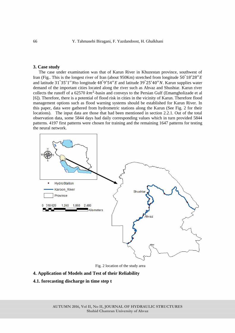
Y. Tahmasebi Biragani, F. Yazdandoost, H. Ghalkhani
AUTUMN 2016, Vol II, No II, JOURNAL OF HYDRAULIC STRUCTURES
Shahid Chamran University of Ahvaz
66
3. Case study The case under examination was that of Karun River in Khuzestan province, southwest of
Iran (Fig.. This is the longest river of Iran (about 950Km) stretched from longitude 50°18′28′′𝐸
and latitude 31°35′1′′𝑁to longitude 48°9′54′′𝐸 and latitude 39°25′40′′𝑁. Karun supplies water
demand of the important cities located along the river such as Ahvaz and Shushtar. Karun river
collects the runoff of a 62570 𝑘𝑚2-basin and conveys to the Persian Gulf (Emamgholizade et al
[6]). Therefore, there is a potential of flood risk in cities in the vicinity of Karun. Therefore flood
management options such as flood warning systems should be established for Karun River. In
this paper, data were gathered from hydrometric stations along the Karun (See Fig. 2 for their
locations). The input data are those that had been mentioned in section 2.2.1. Out of the total
observation data, some 5844 days had daily corresponding values which in turn provided 5844
patterns. 4197 first patterns were chosen for training and the remaining 1647 patterns for testing
the neural network.
Fig. 2 location of the study area
4. Application of Models and Test of their Reliability
4.1. forecasting discharge in time step t
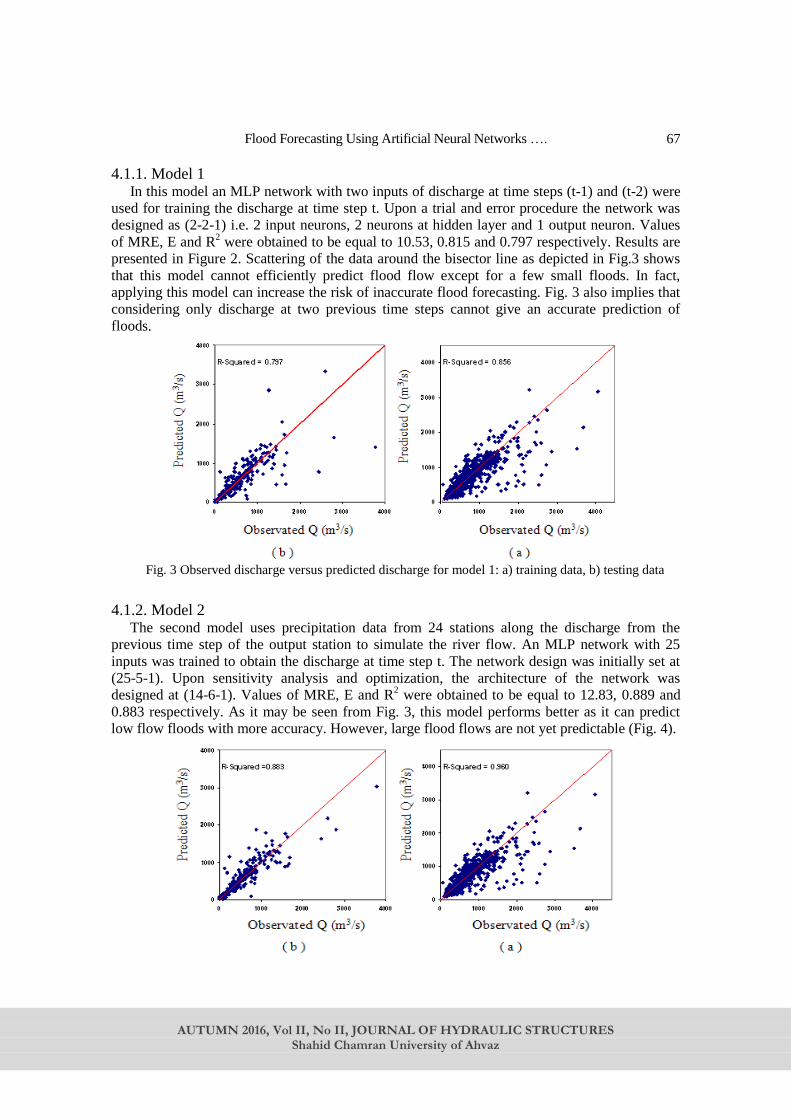
Flood Forecasting Using Artificial Neural Networks ….
AUTUMN 2016, Vol II, No II, JOURNAL OF HYDRAULIC STRUCTURES
Shahid Chamran University of Ahvaz
67
4.1.1. Model 1 In this model an MLP network with two inputs of discharge at time steps (t-1) and (t-2) were
used for training the discharge at time step t. Upon a trial and error procedure the network was
designed as (2-2-1) i.e. 2 input neurons, 2 neurons at hidden layer and 1 output neuron. Values
of MRE, E and R2 were obtained to be equal to 10.53, 0.815 and 0.797 respectively. Results are
presented in Figure 2. Scattering of the data around the bisector line as depicted in Fig.3 shows
that this model cannot efficiently predict flood flow except for a few small floods. In fact,
applying this model can increase the risk of inaccurate flood forecasting. Fig. 3 also implies that
considering only discharge at two previous time steps cannot give an accurate prediction of
floods.
Fig. 3 Observed discharge versus predicted discharge for model 1: a) training data, b) testing data
4.1.2. Model 2 The second model uses precipitation data from 24 stations along the discharge from the
previous time step of the output station to simulate the river flow. An MLP network with 25
inputs was trained to obtain the discharge at time step t. The network design was initially set at
(25-5-1). Upon sensitivity analysis and optimization, the architecture of the network was
designed at (14-6-1). Values of MRE, E and R2 were obtained to be equal to 12.83, 0.889 and
0.883 respectively. As it may be seen from Fig. 3, this model performs better as it can predict
low flow floods with more accuracy. However, large flood flows are not yet predictable (Fig. 4).
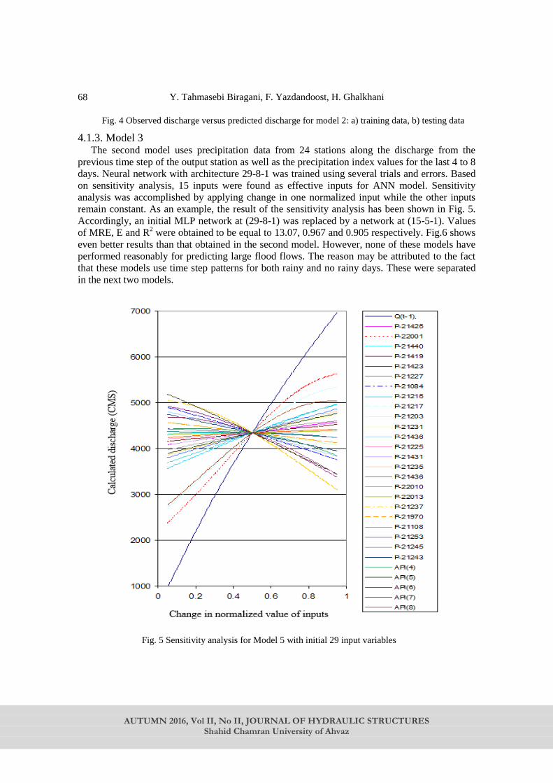
Y. Tahmasebi Biragani, F. Yazdandoost, H. Ghalkhani
AUTUMN 2016, Vol II, No II, JOURNAL OF HYDRAULIC STRUCTURES
Shahid Chamran University of Ahvaz
68
Fig. 4 Observed discharge versus predicted discharge for model 2: a) training data, b) testing data
4.1.3. Model 3 The second model uses precipitation data from 24 stations along the discharge from the
previous time step of the output station as well as the precipitation index values for the last 4 to 8
days. Neural network with architecture 29-8-1 was trained using several trials and errors. Based
on sensitivity analysis, 15 inputs were found as effective inputs for ANN model. Sensitivity
analysis was accomplished by applying change in one normalized input while the other inputs
remain constant. As an example, the result of the sensitivity analysis has been shown in Fig. 5.
Accordingly, an initial MLP network at (29-8-1) was replaced by a network at (15-5-1). Values
of MRE, E and R2 were obtained to be equal to 13.07, 0.967 and 0.905 respectively. Fig.6 shows
even better results than that obtained in the second model. However, none of these models have
performed reasonably for predicting large flood flows. The reason may be attributed to the fact
that these models use time step patterns for both rainy and no rainy days. These were separated
in the next two models.
Fig. 5 Sensitivity analysis for Model 5 with initial 29 input variables
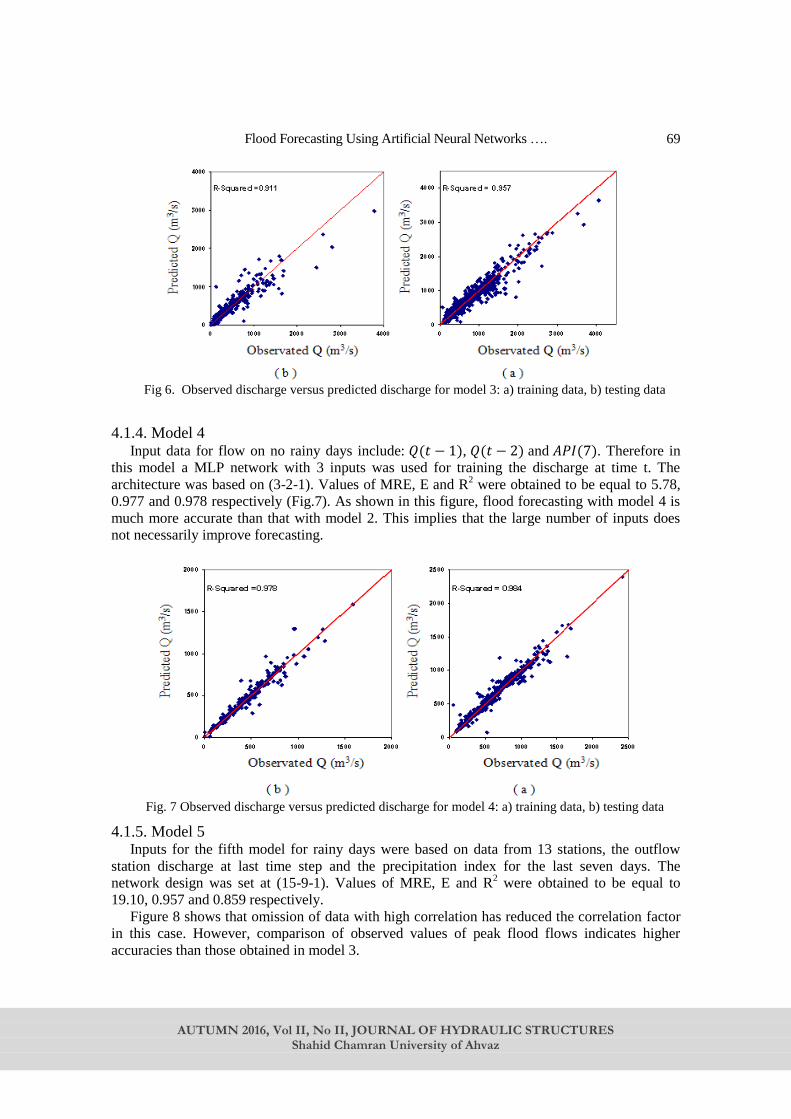
Flood Forecasting Using Artificial Neural Networks ….
AUTUMN 2016, Vol II, No II, JOURNAL OF HYDRAULIC STRUCTURES
Shahid Chamran University of Ahvaz
69
Fig 6. Observed discharge versus predicted discharge for model 3: a) training data, b) testing data
4.1.4. Model 4 Input data for flow on no rainy days include: 𝑄(𝑡 − 1), 𝑄(𝑡 − 2) and 𝐴𝑃𝐼(7). Therefore in
this model a MLP network with 3 inputs was used for training the discharge at time t. The
architecture was based on (3-2-1). Values of MRE, E and R2 were obtained to be equal to 5.78,
0.977 and 0.978 respectively (Fig.7). As shown in this figure, flood forecasting with model 4 is
much more accurate than that with model 2. This implies that the large number of inputs does
not necessarily improve forecasting.
Fig. 7 Observed discharge versus predicted discharge for model 4: a) training data, b) testing data
4.1.5. Model 5 Inputs for the fifth model for rainy days were based on data from 13 stations, the outflow
station discharge at last time step and the precipitation index for the last seven days. The
network design was set at (15-9-1). Values of MRE, E and R2 were obtained to be equal to
19.10, 0.957 and 0.859 respectively.
Figure 8 shows that omission of data with high correlation has reduced the correlation factor
in this case. However, comparison of observed values of peak flood flows indicates higher
accuracies than those obtained in model 3.

Y. Tahmasebi Biragani, F. Yazdandoost, H. Ghalkhani
AUTUMN 2016, Vol II, No II, JOURNAL OF HYDRAULIC STRUCTURES
Shahid Chamran University of Ahvaz
70
Fig. 8 Observed discharge versus predicted discharge for model 5: a) training data, b) testing data
4.1.6. Combination of Model 4 and Model 5 The combined model may be readily compared with any individual model. Values of MRE, E
and R2 were obtained to be equal to 9.10, 0.913 and 0.911 respectively. As may be seen in Fig.
9, this combined model can predict the flood hydrographs more accurately than the first three
models. Flood predictions are made more accurately whilst both rainy and no rainy days have
been considered. For more simple comparison, errors and R2 have been listed in table 1.
Fig. 9 Observed discharge versus predicted discharge for combined model: a) training data, b) testing data
Table 1. The value of errors for models
MRE E R2
Model Test Training Test Training Test Training
10.53 7.87 0.815 0.862 0.897 0.856 1st
12.83 6.69 0.889 0.959 0.883 0.96 2nd
13.07 8.61 0.967 0.948 0.905 0.946 3rd
5.78 2.92 0.977 0.999 0.978 0.984 4th
19.10 10.96 0.957 0.999 0.859 0.957 5th
9.10 5.76 0.913 0.971 0.911 0.969 Combined
model
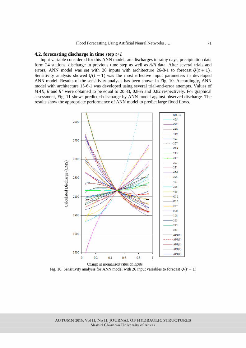
Flood Forecasting Using Artificial Neural Networks ….
AUTUMN 2016, Vol II, No II, JOURNAL OF HYDRAULIC STRUCTURES
Shahid Chamran University of Ahvaz
71
4.2. forecasting discharge in time step t+1 Input variable considered for this ANN model, are discharges in rainy days, precipitation data
form 24 stations, discharge in previous time step as well as 𝐴𝑃𝐼 data. After several trials and
errors, ANN model was set with 26 inputs with architecture 26-8-1 to forecast 𝑄(𝑡 + 1) .
Sensitivity analysis showed 𝑄(𝑡 − 1) was the most effective input parameters in developed
ANN model. Results of the sensitivity analysis has been shown in Fig. 10. Accordingly, ANN
model with architecture 15-6-1 was developed using several trial-and-error attempts. Values of
𝑀𝐴𝐸, 𝐸 and 𝑅2 were obtained to be equal to 20.83, 0.865 and 0.82 respectively. For graphical
assessment, Fig. 11 shows predicted discharge by ANN model against observed discharge. The
results show the appropriate performance of ANN model to predict large flood flows.
Fig. 10. Sensitivity analysis for ANN model with 26 input variables to forecast 𝑄(𝑡 + 1)

Y. Tahmasebi Biragani, F. Yazdandoost, H. Ghalkhani
AUTUMN 2016, Vol II, No II, JOURNAL OF HYDRAULIC STRUCTURES
Shahid Chamran University of Ahvaz
72
Fig. 11. Observed discharge versus predicted discharge for forecasting 𝑄(𝑡 + 1): a) training data, b)
testing data
4. Conclusion Establishing an accurate flood warning system is vital option for timely flood management.
Artificial neural network are typically considered as a suitable method to model physical
phenomena such as riverine flood forecasting. However, determination of the effective inputs for
ANN modelling is significant. In this research a neural network model and a data fusion
technique were used to predict flood flows in the Karun River. Five ANN models were
developed with different inputs combinations. Data for the fourth and fifth model were
combined based on input variables for discharge, precipitation and the precipitation index for the
previous seven days. In spite of variety of input data, the resulting model showed greater
accuracy in predicting floods compared to models with less variety of input variables. Sensitivity
tests were utilized to omit inputs with less effects on prediction of floods resulting in even
greater accuracy.
Notations 𝑋= vector of predictors
𝑌= forecast variable
𝜀 =model error
𝑛= number of observation data
[𝑌]= matrix of estimations of 𝑦 provided by different individual models
𝑛𝑒𝑡𝑗 = the net input information arriving at node 𝑗
𝑤𝑖𝑗 = the connection strength or weight between nodes 𝑖 and 𝑗
𝑜𝑖= the activation at node 𝑖 𝑜𝑗= the output at node 𝑗
𝑃= the total number of patterns in the training set
𝐾= the total number of output nodes,
𝑑𝑝𝑘 and 𝑜𝑝𝑘 = the desired and calculated outputs at node 𝑗 for pattern 𝑝
𝑋𝑛 = the normalized value of input 𝑋
𝑋𝑚𝑖𝑛= the minimum of the input 𝑋
𝑋𝑚𝑎𝑥 = the maximum of the input 𝑋.
𝐸 = Nash-Sutcliffe parameter

Flood Forecasting Using Artificial Neural Networks ….
AUTUMN 2016, Vol II, No II, JOURNAL OF HYDRAULIC STRUCTURES
Shahid Chamran University of Ahvaz
73
𝑀𝑅𝐸 = mean relative error
𝑅= correlation coefficient
𝑄𝑜𝑏𝑠𝑖 = 𝑖th observed discharge
𝑄𝑠𝑖𝑚𝑖 = 𝑖th simulated discharge
𝑛 = the number of data.
𝑄 = the discharge
𝑃= the precipitation
𝑇= the temperature
)(xAPI = the previous precipitation index at previous x time steps and
𝑡 = the computational time step
K = the precipitation constant varying between
jxP = the precipitation at day jx
ET = the evapotranspiration
Wm= the maximum available soil moisture for evaporation.
References 1. Abart, R., SEE, L. (2002) Multi-model data fusion for river flow forecasting: an valuation of
six alternative methods based on two contrasting catchment. Hydrology and Earth System
Sciences 6(4): 655-670.
2. Araghinejad,S., Azmi, M., Kholghi, M., (2011) Application of artificial neural network
ensembles in probabilistic hydrological forecasting. Journal of Hydrology 407(1-4): 94-104.
3. Chen, C., Chen, B., Chou, F., Yang, C., (2010) Development and application of a decision
group Back-Propagation Neural Network for flood forecasting. Journal of Hydrology 385:
173–182.
4. Dasarathy, B. V. (1997) Sensor fusion potential explotation-innovative architectures and
illustrative applications. Proceeding of the IEEE 85: 24-38.
5. Demeritt, D. et al., (2007) Ensemble predictions and perceptions of risk, uncertainty and error
in flood forecasting. Environmental Hazards 7(2): 115.-127.
6. Emamgholizade, S., Kashi, H., Maroofpoor, I., Zalghi, E. (2014) Prediction of water quality
parameters of Karoon River (Iran) by artificial intelligence-based models. International
Journal of Environmental Science and Technology 11(3): 645-656.
7. French, M. N., Krajewshi, W. F., and Cuendall, P. P., (1992) Rainfall Forecasting in Space
and Time using Artificial Neural Networks, Journal of Hydrology 137: 1-31.
8. Hall, D. L. (1992) Mathematical technique in multi-sensor data fusion. Artech House,
Boston,MA.
9. See, L., Abrahart, R. J. (2001) Multi-model data fusion for hydrological forecasting, Comput..
Geosci. 27: 987-994.
10. Shu, C., Burn, D. H., (2004) Artificial neural network ensembles and their application in
pooled flood frequency analysis. Water Resour. Res. 40(9): W09301.
11. Sudheer, K.P., Jain, A., (2004) Explaining the internal behavior of artificial neural network
river flow models. Hydrological Processes 18 (4): 833–844.
12. Van Berkom, F., Van de Watering, C., de Gooijer, K., Neher, A., (2007) Inventory of flood
information systems in Europe – a study of available systems in Western-, Central- and
Eastern Europe, INTERREG IIIC Network Flood Awareness and Prevention Policy in
Border Areas’ (FLAPP), The Netherlands.
AUTUMN 2016, Vol II, No II, JOURNAL OF HYDRAULIC STRUCTURES
Shahid Chamran University of Ahvaz
Journal of Hydraulic Structures
J. Hydraul. Struct., 2016; 2(2):74-84
DOI: 10.22055/jhs.2016.12874
Estimation of Sediment Transport Rate of Karun River (Iran)
Navideh Najafpour 1
Samad Emamgholizadeh 2
Hasan Torabi poudeh3
Amir Hamzeh Haghiabi4
Abstract Several types of sediment transport equations have been developed for estimation of the river
sediment materials during the past decades. The estimated sediment from these equations is very
different, especially when they applied for a specific river. Therefore, choice of an equation for
estimation of the river sediment load is not an easy task. In this study 10 important sediment
transport equations namely; Meyer-Peter and Muller (1948), Einstein (1950), Bagnold (1966),
Engelund and Hansen (1972), Toffaleti (1969), Yang (1996), Van Rijn (2004), Wiuff (1985),
Samaga et al. (1986) and Beg (1995) are used to estimate sediment load of the Karun River in
Iran. The estimated sediment load compared with the measured field data by using statistical
criteria such as root mean square error (RMSE), mean absolute error (MAE) and correlation
coefficient (R2). Results showed that Engelund and Hansen formula can provide reliable
estimates of sediment load of the Karun River which have high suspended sediment load
concentration with RMSE of 3725 ton/day, MAE of 1058.82 ton/day and R2 of 0.41. Bagnold and
Wiuff formulas estimated the total sediment load 280 % and 700% more than the measured
values and the Van Rijn, Tofaleti and Bagnold formulas estimated the sediment load 99 %, 71%
and 93 % lower than the measured values, respectively. The comparison indicated that Samaga,
Einstein, Tofaleti and Yang equations with low accuracy are not suitable for estimation of
sediment load of the Karun River. The main reason for this difference is related to fact that the
Karun River carries fine sediment (wash load) which these equations not considered it.
Keywords: Sediment, Suspended load, bed load, transport formula, Karun River
Received: 09 July 2016; Accepted: 25 November 2016
1 Ph.D. Student in Water Engineering, Lorestan University, Iran, [email protected]
2 Associate Professor, Department of Water and Soil Engineering, Shahrood University of Technology,
Iran. [email protected] (Corresponding author)
3 Assistant Professor, Department of Water Engineering, Lorestan University, KhoramAbad, Iran.
4 Professor, Department of Water Engineering, Lorestan University, KhoramAbad, Iran.
Estimation of Sediment Transport Rate of Karun River
AUTUMN 2016, Vol II, No II, JOURNAL OF HYDRAULIC STRUCTURES
Shahid Chamran University of Ahvaz
75
1. Introduction Since natural rivers are subject to constant erosion and sediment transport processes, the
study of sediment transport mechanisms and sediment transport capacity of stream flows is
considerably important in hydraulics and morphology behaviors of a river (Sheppard, 1963;
Roushangar et al., 2014). Sediment transport and sedimentation in rivers have serious outcomes
that lead to formation of sediment bars and therefore reduction of flood capacity (Cazanacli et
al., 2002), reduction the reservoir capacity and its lifetime (Hassanzadeh et al., 2011) and severe
erosion of hydro mechanical facilities (Ghomeishi and Hemadi, 2007). Also erosion and
deposition along the river change the morphology of river and as result the cross section,
stability and the capacity of rivers will change (Habibi, 1994; Kiat et al., 2008). Various
equations such as mathematical modeling, physical modeling or both are used by investigators to
study of sediment transport, river hydraulics, and river channel changes (Kiatet al., 2008).
Sediment transport in natural rivers has been widely studied in the past few decades and there
are many theoretical or empirical formulas that can be used with reasonable accuracy to predict
the sediment transport rate for sand bed river. For example, the sediment transport equations
developed by Bagnold (1966), Engelund and Hansen (1972), Yang (1996) and Van Rijn (2004)
are often applied to compute bed- material load in rivers.
The significant difference between results obtained by different formulas emphasizes the
necessity of assessing predicted values by different formulas in varying river conditions (Yang,
1996). As the existing formulas predict the maximum sediment transport capacity of a river, so
the measured sediment load may be less than the calculated sediment loads by these formulas. A
large number of comparison studies have been done to test the predictability of various
sediment transport equations covering a wide range of flow conditions and sediment types,
but the accuracy of computational sediment transport models has remained a “challenging
question” yet (ASCE, 2004). For selecting the most proper equations for estimation of sediment
discharge for a river, it is necessary to evaluate them. The literature review show that different
studies were performed to predict the suspended sediment load (Wu et al., 2008; Zhang et al.,
2012; Heidarnejad, and Gholami, 2012), bed load(Yang and Wan, 1991; Sirdari et al., 2001;
Haddadchi et al., 2013) and total load (Wu et al., 2008; Roushangar et al., 2014) of rivers.
For example Cea et al. (2014) used different sediment transport formulations (Meyer-Peter
and Muller (1948), Wong–Parker (2003), Einstein-Brown (1950), van Rijn (1984), Engelund
and Hansen (1967), Ackers-White (1973), Yang (1973), and a Meyer-Peter and Muller), which
commonly used in morphological studies in rivers. Also they analyzed the relevance of
corrections on the sediment flux direction and magnitude due to the bed slope and the non-
equilibrium hypothesis. Haddadchi et al. (2013) evaluated the ability of twelve bed load
sediment transport equations with two types of grain size namely bed load and bed material. For
this purpose they used field data which collected by handheld bed load sampler in Narmab
River, northeastern Iran. They showed that the best results when achieved the bed load grain size
were used to the equations of Shocklitsch, Meyer-Peter and Mueller, while the equations of
Engelund and Hansen, Van Rijn and Einstein perform well with bed material grain size.
The Karun River is the main important river in Iran. The present paper aims is to evaluate the
ability and performance of the ten commonly used sediment transport formulas to prediction the
sediment transport capacity of this river.
2. Data, Methods and Models
2.1. Study sites and data The study area is located in the Karun River Basin, Iran (Fig. 1). The Karun River is the
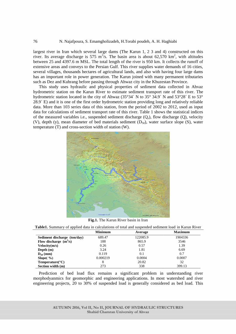
N. Najafpoura, S. Emamgholizadeh, H.Torabi poudeh, A. H. Haghiabi
AUTUMN 2016, Vol II, No II, JOURNAL OF HYDRAULIC STRUCTURES
Shahid Chamran University of Ahvaz
76
largest river in Iran which several large dams (The Karun 1, 2 3 and 4) constructed on this
river. Its average discharge is 575 m3/s. The basin area is about 62,570 km
2, with altitudes
between 25 and 4397.6 m MSL. The total length of the river is 950 km. It collects the runoff of
extensive areas and conveys to the Persian Gulf. This river supplies water demands of 16 cities,
several villages, thousands hectares of agricultural lands, and also with having four large dams
has an important role in power generation. The Karun joined with many permanent tributaries
such as Dez and Kuhrang before passing through Ahwaz city in the Khuzestan Province.
This study uses hydraulic and physical properties of sediment data collected in Ahvaz
hydrometric station on the Karun River to estimate sediment transport rate of this river. The
hydrometric station located in the city of Ahwaz (35°34´ N to 35° 34.9´ N and 53°28´ E to 53°
28.9´ E) and it is one of the first order hydrometric station providing long and relatively reliable
data. More than 103 series data of this station, from the period of 2002 to 2012, used as input
data for calculations of sediment transport rate of this river. Table 1 shows the statistical indices
of the measured variables i.e., suspended sediment discharge (Qs), flow discharge (Q), velocity
(V), depth (y), mean diameter of bed materials sediment (D50), water surface slope (S), water
temperature (T) and cross-section width of station (W).
Fig.1. The Karun River basin in Iran
Table1. Summary of applied data in calculations of total and suspended sediment load in Karun River
Minimum Average Maximum
Sediment discharge (ton/day) 689.47 122085.9 1904336
Flow discharge (m3/s) 188 865.9 3546
Velocity(m/s) 0.26 0.57 1.39
Depth (m) 3.24 1.81 6.69
D50 (mm) 0.119 0.1 0.7
Slope) %( 0.000219 0.0004 0.0007
Temperature(°C) 8 20.82 32
Section width (m) 273 338 399.13
Prediction of bed load flux remains a significant problem in understanding river
morphodyanmics for geomorphic and engineering applications. In most watershed and river
engineering projects, 20 to 30% of suspended load is generally considered as bed load. This
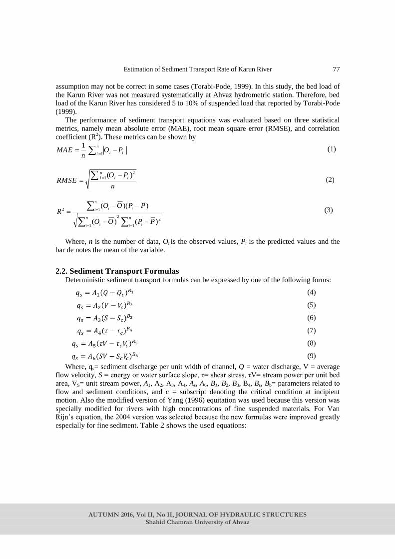
Estimation of Sediment Transport Rate of Karun River
AUTUMN 2016, Vol II, No II, JOURNAL OF HYDRAULIC STRUCTURES
Shahid Chamran University of Ahvaz
77
assumption may not be correct in some cases (Torabi-Pode, 1999). In this study, the bed load of
the Karun River was not measured systematically at Ahvaz hydrometric station. Therefore, bed
load of the Karun River has considered 5 to 10% of suspended load that reported by Torabi-Pode
(1999).
The performance of sediment transport equations was evaluated based on three statistical
metrics, namely mean absolute error (MAE), root mean square error (RMSE), and correlation
coefficient (R2). These metrics can be shown by
1
1 n
i iiMAE O P
n (1)
2
1( )n
i i iO PRMSE
n
(2)
n
i i
n
i i
n
i ii
PPOO
PPOOR
1
22
1
12
)()(
))(( (3)
Where, n is the number of data, Oi is the observed values, Pi is the predicted values and the
bar de notes the mean of the variable.
2.2. Sediment Transport Formulas Deterministic sediment transport formulas can be expressed by one of the following forms:
𝑞𝑠 = 𝐴1(𝑄 − 𝑄𝑐)𝐵1 (4)
𝑞𝑠 = 𝐴2(𝑉 − 𝑉𝑐)𝐵2 (5)
𝑞𝑠 = 𝐴3(𝑆 − 𝑆𝑐)𝐵3 (6)
𝑞𝑠 = 𝐴4(𝜏 − 𝜏𝑐)𝐵4 (7)
𝑞𝑠 = 𝐴5(𝜏𝑉 − 𝜏𝑐𝑉𝑐)𝐵5 (8)
𝑞𝑠 = 𝐴6(𝑆𝑉 − 𝑆𝑐𝑉𝑐)𝐵6 (9)
Where, qs= sediment discharge per unit width of channel, Q = water discharge, V = average
flow velocity, S = energy or water surface slope, τ= shear stress, τV= stream power per unit bed
area, VS= unit stream power, A1, A2, A3, A4, As, A6, B1, B2, B3, B4, Bs, Bb= parameters related to
flow and sediment conditions, and c = subscript denoting the critical condition at incipient
motion. Also the modified version of Yang (1996) equitation was used because this version was
specially modified for rivers with high concentrations of fine suspended materials. For Van
Rijn’s equation, the 2004 version was selected because the new formulas were improved greatly
especially for fine sediment. Table 2 shows the used equations:

N. Najafpoura, S. Emamgholizadeh, H.Torabi poudeh, A. H. Haghiabi
AUTUMN 2016, Vol II, No II, JOURNAL OF HYDRAULIC STRUCTURES
Shahid Chamran University of Ahvaz
78
Table 2. Equations which used for calculation of sediment load in Karun River Researcher Equation
Bagnold (1966) tanb b
S
q V e
Engelund and Hansen (1972)
2 1/2 3/250 0
50
0.05 ( ) ( )( 1) ( )
t s
s s
dq V
g G d
Yang (1996)
𝐿𝑜𝑔𝐶𝑡 =
5.165 − 0.153𝐿𝑜𝑔𝜔𝑚𝑑50
𝜈− 0.297𝐿𝑜𝑔
𝑉∗
𝜔𝑚+ (1.78 −
0.36 𝐿𝑜𝑔𝜔𝑚𝑑50
𝜈−0.48 𝐿𝑜𝑔
𝑉∗
𝜔𝑚)𝐿𝑜𝑔 [
𝑉𝑆
𝜔𝑚
𝛾𝑚
(𝛾𝑠−𝛾𝑚)]
Van Rijn (2004) 𝑞𝑏 = 𝛾 𝜌𝑠 𝑓𝑠𝑖𝑙𝑡 𝑑50 𝑑∗−0.3 (
𝜏𝑏,𝑐𝑤′
𝜌)
0.5
[𝜏𝑏,𝑐𝑤
′ −𝜏𝑏,𝑐𝑟
𝜏𝑏,𝑐𝑟]
𝜂
Meyer-Peter Muller and
derivatives (1948)
3/2 1/3 2/3
2/3
1
0.047 0.25s s ss m b
r
n
m si
i
Q Kd S D q
Q K g
D D i
where γ and γs are specific weights of water and sediment, respectively, qb is bed
load transport rate per unit width, tan α is the ratio of tangential to normal shear force, 𝜏 is
shear stress along the bed, eb is the efficiency coefficient, V is the average flow velocity;
tq is total sediment discharge by weight per unit width, d50 is the mean diameter of the bed
materials; g is the gravitational acceleration; Gs is the specific gravity given by γ
γs ; fsilt is a
silt factor; τbcr is the instantaneous grain related bed-shear stress due to both currents and
waves; ρb is the critical bed-shear stress according to shields; ρ is the density of water; is
the dimensionless particle size; Ct tis the weight concentration of sediment in ppm; ωm is
particle fall velocity; QS id the part of the water discharge apportioned to the bed; Q is the
total water discharge; KS = Strickler's coefficient of bed roughness; Kr = the coefficient of
particle roughness; d is the mean depth; S is the energy gradient; Dm is the effective
diameter of bed-material mixture; n is the number of size fractions in the bed material, Dsi =
the mean grain diameter of the sediment in size fraction i, and ih.
3. Results and Discussion The total sediment load of Karun River was calculated by the selected formulas namely
Meyer-Peter and Muller, Engelund and Hansen, Yang and Beg while suspended load were
calculated by Bagnold, Van Rijn, Toffaleti, Einstein, Samaga et al and Wiuff equations.
Since at Ahvaz hydrometric station only the suspended load is measured, therefore for
calculating total load, 5 - 10 % of suspended load considered as bed load. For comparing the
measured and calculated sediment loads, in addition to RMASE, MAE and R2, the ratio of R
(R=calculated load/ measured load) are used. The results are shown in Table 3. Also the
calculated sediment load compared with field measurement data in Fig. 2.
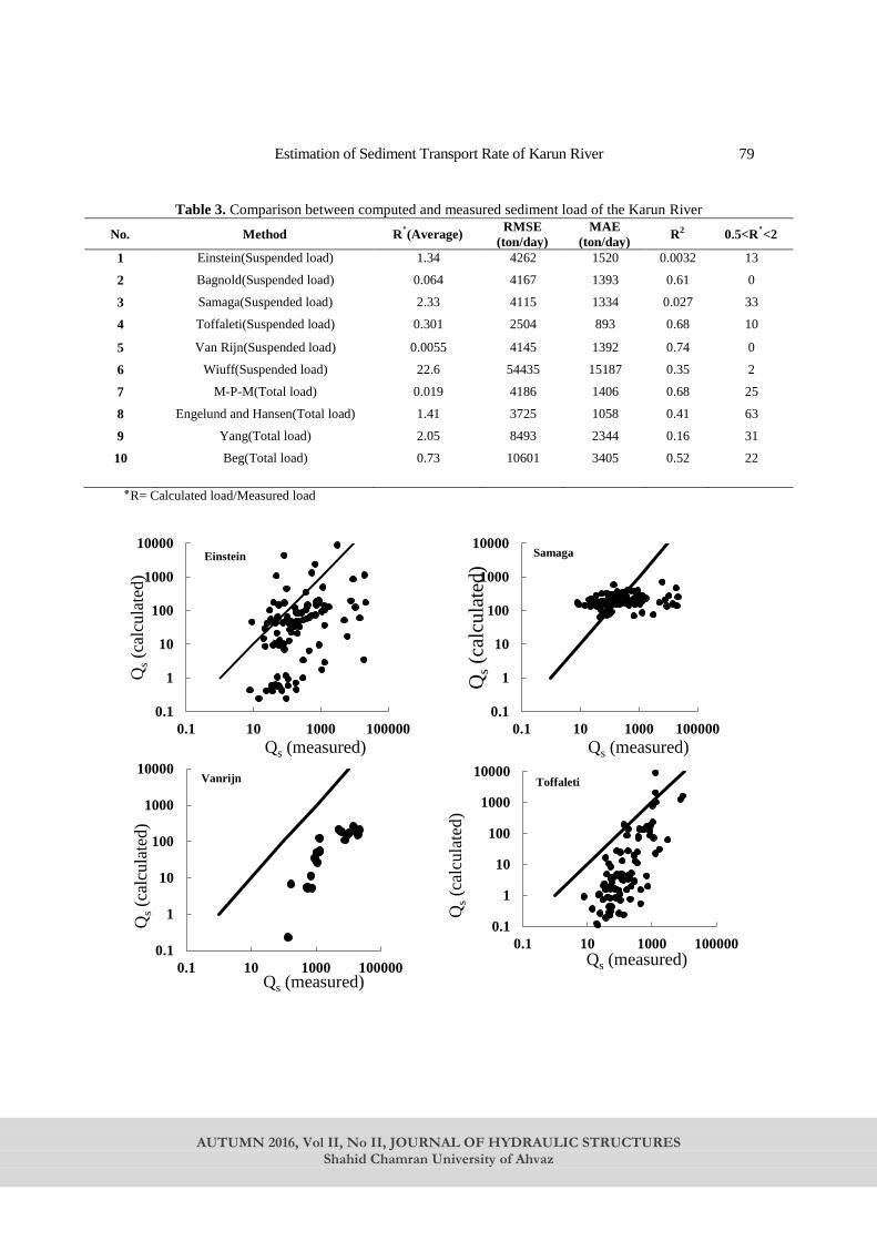
Estimation of Sediment Transport Rate of Karun River
AUTUMN 2016, Vol II, No II, JOURNAL OF HYDRAULIC STRUCTURES
Shahid Chamran University of Ahvaz
79
Table 3. Comparison between computed and measured sediment load of the Karun River
No. Method R٭(Average) RMSE
(ton/day)
MAE
(ton/day) R2 0.5<R2>٭
1 Einstein(Suspended load) 1.34 4262 1520 0.0032 13
2 Bagnold(Suspended load) 0.064 4167 1393 0.61 0
3 Samaga(Suspended load) 2.33 4115 1334 0.027 33
4 Toffaleti(Suspended load) 0.301 2504 893 0.68 10
5 Van Rijn(Suspended load) 0.0055 4145 1392 0.74 0
6 Wiuff(Suspended load) 22.6 54435 15187 0.35 2
7 M-P-M(Total load) 0.019 4186 1406 0.68 25
8 Engelund and Hansen(Total load) 1.41 3725 1058 0.41 63
9 Yang(Total load) 2.05 8493 2344 0.16 31
10 Beg(Total load) 0.73 10601 3405 0.52 22
R= Calculated load/Measured load٭
0.1
1
10
100
1000
10000
0.1 10 1000 100000
Qs
(cal
cula
ted)
Qs (measured)
Einstein
0.1
1
10
100
1000
10000
0.1 10 1000 100000
Qs
(cal
cula
ted)
Qs (measured)
Samaga
0.1
1
10
100
1000
10000
0.1 10 1000 100000
Qs
(cal
cula
ted)
Qs (measured)
Vanrijn
0.1
1
10
100
1000
10000
0.1 10 1000 100000
Qs
(cal
cula
ted)
Qs (measured)
Toffaleti

N. Najafpoura, S. Emamgholizadeh, H.Torabi poudeh, A. H. Haghiabi
AUTUMN 2016, Vol II, No II, JOURNAL OF HYDRAULIC STRUCTURES
Shahid Chamran University of Ahvaz
80
Fig. 2. Comparison between measured and calculated sediment load concentration of The Karun River
From the results of Table 3 and also Fig. 2 it can be concluded that Wiuff equation predicts
the suspended sediment load of the Karun River higher than the measured values with RMSE of
54435 ton/day and R2 of 0.35. While Bagnold and Toffaleti equations predict suspended
sediment load less than measured values with RMSE of 4167 and 2504 ton/day and R2 of 0.61
and 0.68 respectively. The predicted values of sediment load by Einstein, Samaga and Van Rijn
equations are unclear and imprecise (Fig. 2 a, c, e, i).
Beg equation predicts suspended sediment load of the Karun River higher than measured
values with RMSE of 10601 ton/day and R2 of 0.52. Meyer-Peter and Muller equation estimates
total sediment load of the Karun River less than measured values with RMSE of 4186 and R2 of
0.1
1
10
100
1000
0.1 10 1000 100000
Qs
(cal
cula
ted
)
Qs (measured)
Bagnold
0.1
1
10
100
1000
10000
100000
0.1 10 1000 100000
Qs
(cal
cula
ted)
Qs (measured)
Wiuff
0.1
1
10
100
1000
10000
100000
0.1 10 1000 100000
Qs
(cal
cula
ted)
Qs (measured)
Yang
0.1
1
10
100
1000
10000
0.1 10 1000 100000
Qs
(cal
cula
ted)
Qs (measured)
Meyer-Peter and Muller
0.1
1
10
100
1000
10000
100000
0.1 10 1000 100000
Qs (c
alcu
late
d)
Qs (measured)
Beg
0.1
1
10
100
1000
10000
0.1 10 1000 100000
Qs
(cal
cula
ted)
Qs (measured)
Engelund and Hansen

Estimation of Sediment Transport Rate of Karun River
AUTUMN 2016, Vol II, No II, JOURNAL OF HYDRAULIC STRUCTURES
Shahid Chamran University of Ahvaz
81
0.68. The prediction of Yang equation is unclear, while Engelund and Hansen equation is less
imprecise (Fig. 2 h) and seems to produce the best prediction of total sediment load among the
selected equations with RMSE of 3725 and R2 of 0.41.
Overall, no accurate equation exists to determine the best sediment prediction formula since
the use of various statistical methods produce different results. Fig.3 shows the sediment load
ratios (R= calculated load / measured load) with different equations. The depicted points in this
figure closer to R = 1 indicate that the selected equation performs more accurately to estimate
the sediment transport load. Also if the depicted points be scattered in direction of R = 1, the
selected method should be modified by applying a corrective coefficient. Results of Fig. 3 show
that for estimation of suspended and total sediment load of the Karun River, Bagnold equation
and also Beg and Engelund and Hansen equations produced a relatively accurate prediction, so
applying corrective coefficient increased the accuracy of these equations (see Table 4).
0.001
0.01
0.1
1
10
100
0 50 100 150
R
n
Einstein
0.001
0.01
0.1
1
0 50 100 150
R
n
Bagnold
0.001
0.01
0.1
1
10
100
0 50 100 150
R
n
Samaga
0.001
0.01
0.1
1
0 50 100 150
R
n
Toffaleti
0.001
0.01
0.1
1
0 50 100 150
R
n
Van Rijn
0.001
0.01
0.1
1
0 50 100 150
R
n
Wiuff
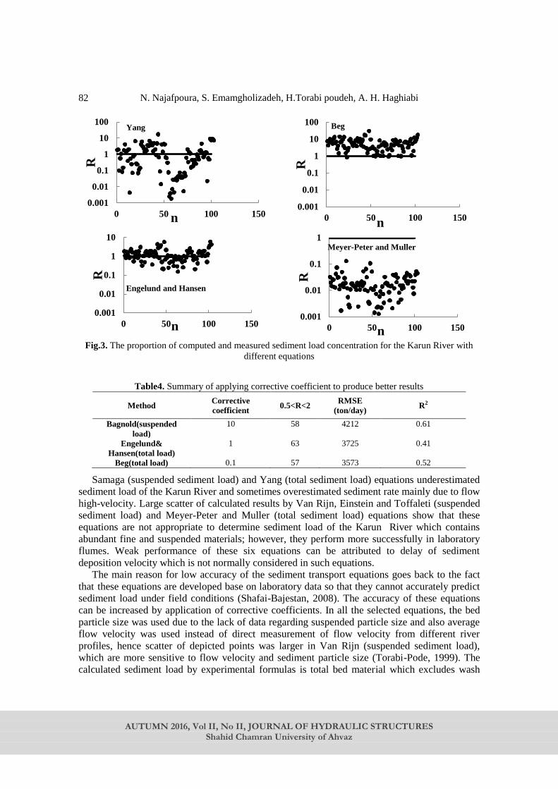
N. Najafpoura, S. Emamgholizadeh, H.Torabi poudeh, A. H. Haghiabi
AUTUMN 2016, Vol II, No II, JOURNAL OF HYDRAULIC STRUCTURES
Shahid Chamran University of Ahvaz
82
Fig.3. The proportion of computed and measured sediment load concentration for the Karun River with
different equations
Table4. Summary of applying corrective coefficient to produce better results
Method Corrective
coefficient 0.5<R<2
RMSE
(ton/day) R2
Bagnold(suspended
load)
10 58 4212 0.61
Engelund&
Hansen(total load)
1 63 3725 0.41
Beg(total load) 0.1 57 3573 0.52
Samaga (suspended sediment load) and Yang (total sediment load) equations underestimated
sediment load of the Karun River and sometimes overestimated sediment rate mainly due to flow
high-velocity. Large scatter of calculated results by Van Rijn, Einstein and Toffaleti (suspended
sediment load) and Meyer-Peter and Muller (total sediment load) equations show that these
equations are not appropriate to determine sediment load of the Karun River which contains
abundant fine and suspended materials; however, they perform more successfully in laboratory
flumes. Weak performance of these six equations can be attributed to delay of sediment
deposition velocity which is not normally considered in such equations.
The main reason for low accuracy of the sediment transport equations goes back to the fact
that these equations are developed base on laboratory data so that they cannot accurately predict
sediment load under field conditions (Shafai-Bajestan, 2008). The accuracy of these equations
can be increased by application of corrective coefficients. In all the selected equations, the bed
particle size was used due to the lack of data regarding suspended particle size and also average
flow velocity was used instead of direct measurement of flow velocity from different river
profiles, hence scatter of depicted points was larger in Van Rijn (suspended sediment load),
which are more sensitive to flow velocity and sediment particle size (Torabi-Pode, 1999). The
calculated sediment load by experimental formulas is total bed material which excludes wash
0.001
0.01
0.1
1
10
100
0 50 100 150
R
n
Yang
0.001
0.01
0.1
1
10
100
0 50 100 150
R
n
Beg
0.001
0.01
0.1
1
10
0 50 100 150
R
n
Engelund and Hansen
0.001
0.01
0.1
1
0 50 100 150
R
n
Meyer-Peter and Muller
Estimation of Sediment Transport Rate of Karun River
AUTUMN 2016, Vol II, No II, JOURNAL OF HYDRAULIC STRUCTURES
Shahid Chamran University of Ahvaz
83
load. On the other hand, with the existence of fine, erosion sensitive formations around the study
area, a large wash load is expected to occur in the Karun River. Thus, the large portion of
difference between measured and calculated sediment load by the selected equations is related to
the washed load of the river. Also, since sediment load is calculated by experimental formulas
for averaged river depth and width while morphological features of a river are different in time,
thus a difference is always expected between the calculated and observed sediment load.
4. Conclusion Various formulas including Einstein, Bagnold, Samaga, Toffaleti, Van Rijn and Wiuff
equations are used to determine suspended sediment load and also Yang, Beg, Englund and
Hansen, Meyer-Peter and Muller equations applied to determine total sediment load of the Karun
River. The 103 series of field data at Ahvaz hydrometric station used and the results were
compared by the measured suspended load. The following conclusions can be drawn:
The best estimation of the Karun River suspended sediment load was produced by Bagnold
method as less erroneous predictions was obtained. In Bagnold equation due to less scattered
points around R = 1(calculated/measured load), a corrective coefficient of 10 can be used to
obtain better result.
Also, for estimation of total sediment load of the Karun River the best prediction were
obtained by Englund and Hansen and Beg equations. In the Beg equation due to less scattered
points around R = 1(calculated/measured load), a corrective coefficient of 0.1 can be used to
obtain better result. Extreme scatter of results by Einstein, Yang and Samaga equations in the
study area shows that such equations were not proper to predict sediment load material of the
Karun River and the coefficient applied in these formulas, which were obtained on lab flumes,
are not good to be used for natural rivers.
The results produced by different formulas were considerably different than the observed
values which can be related to the wash load which none of experimental formulas considered it.
References
1. ASCE Task Committee of Computational Modeling of Sediment transport Processes.
“Computational modeling of sediment transport processes. J. of Hydraul. Eng., 130(7): 597-
598 (2004.).
2. Bagnold, R.A. “An approach to the sediment transport problem from general physics. U.S.
Geol, Survey prof, Paper 4221, Washington, USA (1996).
3.Cea, L. Bladé, L. Corestein, G. Fraga, I. Espinal, M. and Puertas, J. “Comparative analysis of
several sediment transport formulations applied to dam-break flows over erodible beds”, J.
of Hydraul. Res., 50(4), pp. 364-375 (2014).
4. Engelund, F. and E. Hansen. “A Monograph on sediment transport in Alluvial Streams”,
Teknish Forlag, Copenhagen (1972).
5. Ghomeishi, M. and Hemadi, K. “Determination of gradation suspended sediment and relation
between suspended material and flow hydraulic parameters in province Khuzestan Rivers.
Design researches of water and electricity organ of Khuzestan”, In Persian, pp: 178 (2007).
6. Habibi, M. “Sediment transport estimation methods in river systems”, Doctor of Philosophy
thesis, Department of Civil and Mining Engineering, University of Wollongong (1994).
7. Haddadchi, A. Omid, M.H. Dehghani, A.A. “Bed load equation analysis using bed load-
material grain size”, J. Hydrol. Hydromech. 61(3): pp. 241–249 (2013).
8. Hassanzadeh, H. Faiznia, S. Shafai Bajestan, M. and Motamed, A. “Estimate of Sediment
N. Najafpoura, S. Emamgholizadeh, H.Torabi poudeh, A. H. Haghiabi
AUTUMN 2016, Vol II, No II, JOURNAL OF HYDRAULIC STRUCTURES
Shahid Chamran University of Ahvaz
84
Transport Rate at Karkheh River in Iran Using Selected Transport Formulas”, World Appl.
Sci. J. 13 (2): pp. 376-384 (2011).
9. Heidarnejad, M. and Gholami, A. “Modeling Suspended Sediments in Dez Basin (Case Study:
The Tale Zang Hydrometric Station) ”, Int. Res. J. of Appl.and Basic Sci., 3 (2), pp. 402-407
(2012).
10. Kiat, C.C. Ghani, A.A. Abdullah, R. Zakaria, N.A. “Sediment transport modeling for Kulim
River . A case study”, J. of Hydro-envi. Res. 2 , 47-59 (2005).
11. Roushangar, K. Vojoudi Mehrabani, F. Shiri, J. “Modeling river total bed material load
discharge using artificial intelligence approaches (based on conceptual inputs) ”, J. of
Hydrol., 514, pp. 114–122 (2014).
12. Martin, Y. “Evaluation of bed load transport formulae using field evidence from the Vedder
River, British Columbia”, Geomorphology, 53, pp. 75–95 (2003).
13. Shafai-Bajestan, M. “Hydraulics of sediment transport (second edition) ”, Shahid Chamran
University Press, Ahwaz, Iran, In Persian, pp: 549 (2008).
14.Sedaei, N. and Honarbakhsh, A. “Suspended sediment estimation formulae analyzing with
Analytical Hierarchy Processing”, Int. J. of Agri. and Crop Sci., IJACS, 16(5): pp. 1765-1774
(2013).
15. Sheppard, J.R. “Methods and their suitability for determining total sediment quantities”,
Proceedings of the Federal Inter Agency Sedimentation Conference (PFISC), Miscellaneous
publication no. 970. Agricultural Research service, USDA Washington, D.C. 32: pp. 272-
287(1963).
16. Sirdari, Z.Z. Ghani, A. and Sirdari, N.Z. “Bed load transport predictions based on field
measurement data by combination of artificial neural network and genetic”, Pollution,1(1):
pp. 85-94 (2014).
17.Torabi-Pode, H. “Rate equations for estimating sediment of the rivers of Khuzestan”,
Master's thesis, University of Chamran, Ahvaz (1999).
18. Van Rijn, L.C. “A unified view of sediment transport by currents and waves, part I: initiation
of motion, bed roughness and bed load transport”, J. Hydrau. Eng., ASCE, 33(6): pp. 649-
667(2007a).
19. Van Rijn, L.C. “A unified view of sediment transport by currents and waves, part
II:Suspended transport”, J. Hydraul. Eng., ASCE, 33(6): pp. 668- 689 (2007b).
20. Yang, C.T. and Wan, S. “Comparisons of selected bed-material load formulas”, J. of
Hydraul. Eng., 117, 8, 973-989 (1991).
21. Yang, C.T. “Sediment Transport: Theory and Practice”, McGraw- Hill Companies, Inc. New
York, USA, (1996).