Full page photo - scu.ac.ir
83
Transcript of Full page photo - scu.ac.ir


AUTUMN 2017, Vol 3, No II, JOURNAL OF HYDRAULIC STRUCTURES
Journal of Hydraulic Structures Department of Civil Engineering Shahid Chamran University of Ahvaz
In the name of GOD

AUTUMN 2017, Vol 3, No II, JOURNAL OF HYDRAULIC STRUCTURES
JORNAL OF
HYDRAULIC STRUCTURES SHAHID CHAMRAN UNIVERSITY OF AHVAZ
Manager: Prof. Hamid R. Ghafouri Editor-in-chief: Dr. Ali Haghighi Editorial coordinator: Dr. Seyed Mohammad Ashrafi Department of Civil Engineering, Engineering Faculty, Shahid Chamran University of Ahvaz, Ahvaz, Iran. Members Prof. Hossein M. V.Samani Civil Engineering Department, Shahid Chamran University of Ahvaz, Ahvaz, Iran Prof. Hamid R. Ghafouri Civil Engineering Department, Shahid Chamran University of Ahvaz, Ahvaz, Iran
Dr. Ali Haghighi Civil Engineering Department, Shahid Chamran University of Ahvaz, Ahvaz, Iran
Prof. Mahmood S. Bajestan Hydraulic Structures Department, Shahid Chamran University of Ahvaz, Ahvaz, Iran
Prof. Saeed R. S. Yazdi Civil Engineering Department, K.N.Toosi University of Technology, Tehran, Iran
Dr. Mohammad S. Pakbaz Civil Engineering Department, Shahid Chamran University of Ahvaz, Ahvaz, Iran
Dr. Arash Adib Civil Engeering Department, Shahid Chamran University of Ahvaz, Ahvaz, Iran
Dr. Mojtaba Labibzadeh Civil Engineering Department, Shahid Chamran University of Ahvaz, Ahvaz, Iran
Prof. Helena M. Ramos Instituto Superior Técnico (IST), University of Lisbon Dr. S. Mohammad Ashrafi Civil Engineering Department, Shahid Chamran University of Ahvaz, Ahvaz, Iran
Dr. S. Abbas Haghshenas Institute of Geophysics, University of Tehran | UT, Tehran, Iran
Dr. Mohammad Zounemat-Kermani Department of Water Engineering, Shahid Bahonar University of Kerman, Kerman, Iran
Dr. Taher Rajaee Civil Engineering Department, University of Qom, Qom, Iran
Dr. Mohammad Vaghefi Civil Engineering Department, Faculty of Engineering, Persian Gulf University, Bushehr, Iran
Dr. A. A. Telvari Soil Conservation and Watershed Management Research Institute; Department of Civil Engineering, Islamic Azad University, Ahvaz branch, Ahvaz, Iran
CONTENTS VOL 3, NO II, Autumn 2017
II Aims and Scope
01 Investigating the vulnerability downstream area of Taleghan dam due to dam failure H. Goharnejad; M. Azizkhani; M. Zakeri Niri; S. Moazami
10 An experimental study on hydraulic behavior of free-surface radial flow in coarse-grained porous media A. Rajabi; E. Hatamkhani; J. Sadeghian
22 Three-dimensional numerical modeling of score hole in rectangular side weir with finite volume method S. Ghotbi; A. Abdollahi; M. Azhdari Moghadam
32 Experimental Study of the Effect of Base-level fall at the Beginning of the Bend on Reduction of Scour around a Rectangular Bridge Pier Located in the 180 Degree Sharp Bend M. vaghefi; M. moghanloo; D. Dehghan; A. keshavarz
47 Developing optimal operating reservoir rule-curves in drought periods S. Alahdin; H.R. Ghafouri
62 Finding the Causes and Evaluating Their Impacts on Urmia Lake Crisis Using a Comprehensive Water Resources Simulation Model A. B. Dariane; L. Eamen

AUTUMN 2017, Vol 3, No II, JOURNAL OF HYDRAULIC STRUCTURES
Aims and Scope Hydraulic Structure Journal is an interdisciplinary journal which publishes high-quality peer-
reviewed articles addressing the latest developments and applied methods in construction,
maintenance, management, and operation policy of Hydraulic Structures.
The Journal aims at providing an efficient route to fast-track publication, within 10-12 weeks
after manuscript submission. Manuscripts will be considered for publication in the following
categories: research articles, technical notes, case reports and discussions.
The general areas covered by the Journal include:
Technical and methodological advances in application, design/selection, production,
modification of construction materials
Advances in numerical and analytical methods
Hydro informatics and soft computing
Hydraulic aspects of hydraulic structures
Applied surface and subsurface hydrology and hydrometeorology
Forecasting approaches in water resources engineering
Economic and social aspects of hydraulic structures
Uncertainty analysis and risk management in hydraulics and water resources engineering
Application of Nanotechnology in Hydraulic Structures
Geotechnics of Hydraulic Structures
Damage detection techniques
The following might be considered as hydraulic structures:
Dams and associated structures
River and Watershed Structures
Offshore and Onshore Structures
Irrigation and Drainage Channel Networks
Bridges
Water Storage and Conveyance Structures
Pipelines and Pump Stations
Sewerage Systems
Water and Wastewater Treatment Plants
Historical Water Structures
General Information
Title: Journal of Hydraulic Structures
Subject: Hydraulics and water resources engineering
Coverage area: International
Journal Type: Scientific and technical
License Holder: Shahid Chamran University
Editor-in-Chief: Dr. Ali Haghighi
Manager: Prof. Hamid R. Ghafouri
Editorial coordinator: Dr. Seyed Mohammad Ashrafi
Language Editors: Majid SadollahKhani
Soroosh Kamali
Address: Engineering Faculty,
Shahid Chamran University of
Ahvaz
Phone #: +986113330010-20
(5610 & 5603)
Fax #: +986113337010
Language: English
Email: [email protected]
Website: jhs.scu.ac.ir

AUTUMN 2017, Vol 3, No 2, JOURNAL OF HYDRAULIC STRUCTURES
Shahid Chamran University of Ahvaz
Journal of Hydraulic Structures
J. Hydraul. Struct., 2017; 3(2):1-9
DOI: 10.22055/jhs.2017.13435
Investigating the vulnerability downstream area of Taleghan
dam due to dam failure
Hamid Goharnejad1
Mahyar Azizkhani2
Mahmoud Zakeri Niri3
Saber Moazami4
Abstract Due to the immense damage caused by dam failure, especially dams constructed near large
cities, it is necessary to consider the breaking phenomena as well as studying and designing
different parts of the dam. For this purpose, the hydrograph of the outflow due to dam failure
must be identified according to size of the fracture and then flood routing, and flood zone must
be determined based on the downstream topography and morphology. The integration of
hydraulic models and geographic information system is used to achieve this objective. In this
research the effect of breaking Taleghan storage dam due to the slip of a pile of reservoir
abutment and the creation of current wave toward the dam body as well as the vulnerability
analysis due to the breaking of the dam on downstream lands was studied. At first, Taleghan
dam failure for five different scenarios was modeled using the FLOW-3D numerical software
and then the geometric data of the river was extracted using the ArcGIS software and modeling
the flood due to dam failure was conducted in Hec-GeoRas model. Then, the risk analysis was
performed for each break scenario of Taleghan dam. The results indicated that the maximum
amount of inundation would occur in Razmian city at an approximate distance of 45 kilometers
from Taleghan dam site.
Keywords: Dam breaking, Inundation, Vulnerability, Risk analysis, Taleghan dam.
Received: 17 September 2017; Accepted: 07 November 2017
1 Department of Civil Engineering, Environmental Sciences Research Center, Islamshahr Branch, Islamic
Azad university, Islamshahr, Iran, [email protected] (Corresponding author) 2 Department of Civil Engineering, Environmental Sciences Research Center, Islamshahr Branch, Islamic
Azad university, Islamshahr, Iran, [email protected]. 3 Department of Civil Engineering, Environmental Sciences Research Center, Islamshahr Branch, Islamic
Azad university, Islamshahr, Iran, [email protected] 4
Department of Civil Engineering, Environmental Sciences Research Center, Islamshahr Branch, Islamic
Azad university, Islamshahr, Iran, [email protected]
H. Goharnejad, M. Azizkhani, M. Zakeri N., S. Moazami
AUTUMN 2017, Vol 3, No 2, JOURNAL OF HYDRAULIC STRUCTURES
Shahid Chamran University of Ahvaz
2
1. Introduction Dams are always considered as a potential threat for their downstream areas because of
creation of large water reservoirs. Dam designers attempt to lower vulnerability potentials by
applying safety factors; however, natural and non-natural factors like floods, piping
phenomenon, foundation weakness and exploding can cause a dam to break [1]. The problem of
dam failure and effects of surges on downstream areas attracted many scholars and experts'
attention, after several important dams like Teton were broken [2]. To reduce the effects of a
large reservoir dam failure, it is important to know the changes of hydraulic parameters due to
break in dam, such as depth, speed, flow, and the time when the wave forehead reaches the
downstream area and finally to determine the border and designing the flood zone in order to
reduce the financial losses and casualties. In this regard, in the last few decades, different
researchers have done numerous theoretical and practical studies in order to determine the
mechanism of dam failure and the trends of hydraulic parameters as a function of time and space
[3]. One of the most important methods for erosion control in rivers in these situations is ston
masonery and riprap. A general dimensionless equation for the prediction of maximum particle
size of stable riprap into the tributary channel at river confluences has been developed by
Ghanbari Adivi et al. [4]. Their results showed that the stability number of riprap into the
tributary channel increases with increasing the ratio of tailwater depth to particle size.
Fliervoet et al. [5], Lim [6] and Chiew [7] found that during flooding, the emergence of
various forms such as Ripple and Dune and live bed is natural. These processes, despite the
intersectional structures, can cause inconstancy in these structures. Andam [8] investigated the
changes in speed and number of landing by using HECGeo-RAS model in a research entitled as
the comparison of river regime inside and outside of forest area, and compared the influence of
vegetation on the physical behavior of the flow. He concluded that using the HECGeo-RAS
model can offer researchers suitable numbers to study the diet and other hydraulic characteristics
of river flow. Sholtes [10] used HEC-RAS software to route flood dynamics in rural and urban
areas of Northern California and concluded that the decrease in slope and increase in roughness
of floodplain and river have more influence on flood attenuation. Nagy et al., [11] investigated
the sand grinding attrition and meanders evolution in an answer to Tisza River engineering in
Hungary and found that due to severe attrition in the area and human intervention (performing
engineering projects), this river has reached a balance by shortcuts in its route. However, the
purpose of this article is to investigate and determine the flood plain area. Then the amount of
vulnerability risk over all path of the river for five different scenarios of dam break and for wave
arrival times of 30 and 120 minutes were identified.
2. Methodology The conducted research is presented in details in this section.
2.1. Study area Taleghan dam at 135 km of north west of Tehran with longitude of 50 ̊, 37' to 51 ̊ , 10' and
latitude of 36 ̊, 5' to 36 ̊, 25' is built on Taleghan river in Roshanabdar rural area. Figure 1 shows
the study area, including dam, river, and the topography of area.

Investigating the vulnerability downstream area …
AUTUMN 2017, Vol 3, No 2, JOURNAL OF HYDRAULIC STRUCTURES
Shahid Chamran University of Ahvaz
3
Figure 1. Map of Taleghan river in Taleghan dam downstream
2.2 Physical characteristics of Taleghan river in Taleghan dam downstream In order to perform the model, it is necessary to determine the river characteristics such as the
left and right bank, riverbed, and roughness coefficient of each section. Therefore, after several
field studies and inspections, the required data were determined and entered the model. Then
using the Arc-GIS, the cross sections were provided and entered the model. Considering the high
length of the study area, the distance of cross sections in straight parts of the river was chosen
about 4000 meters and 1500 meters in sudden intersections and arches. Among the factors
affecting the manning coefficient are the grading substrate material, the rippling degree of river,
the relative effect of obstacles, the density of vegetation and morphology form of the river.
Therefore, in order to determine and estimate the manning coefficient in a part of river, it should
be divided to three main parts including the mainstream and flood plains of right and left banks.
Because of the important role of roughness coefficient, the model were calibrated using this
parameter.
2.3 Determining boundary conditions In order to predict the characteristics of the flow in the study period, real boundary conditions
are needed. Boundary condition is in fact representative of the output and input status of the
downstream and upstream flows. It is obvious that expecting the exact characteristics of flow
includes offering correct data in boundaries. In the current research, the introduced boundary
condition for hydraulic model to simulate the hydraulic flow of Taleghan river in downstream of
Taleghan dam, used the normal depth condition in upstream and also normal depth boundary
condition in downstream. The HEC-RAS model can calculate the normal depth using Manning's
equation and the slope of river. After simulation, the hydraulic model identifies the slope and

H. Goharnejad, M. Azizkhani, M. Zakeri N., S. Moazami
AUTUMN 2017, Vol 3, No 2, JOURNAL OF HYDRAULIC STRUCTURES
Shahid Chamran University of Ahvaz
4
suitable level of water in upstream.
2.4 Discharge inflow Five scenarios are defined to investigate embankment dam failure resulting from overtopping.
Inflow volume to the reservoir is different in each scenario. Based on the reviews, minimum
flood volume that overtops and damages the dam body is about 5 MCM. In addition, maximum
flood volume that fully destroys the dam body is about 25 MCM. In the range of 5 to 25 MCM,
flood volumes of 7.5, 9 and 13 MCM have been considered. The charecteristics of scenarios
have been presented in Table 1. ([12])
Table1. Flow modeling conditions for five states of overtopping in Taleghan dam
Scenario Water Height in
Reservoir (m)
Storage
(MCM)
Flood
Volume (m3)
Flood Discharge
(cms)
1 82 420 5.0 54,269
2 82 420 7.5 59,390
3 82 420 9.0 78,913
4 82 420 13.0 89,129
5 82 420 25.0 97,054
2.5 The risk taking theory due to dam failure The researchers consider the three parameters of escape time, velocity, and depth of
flooding as the appropriate criteria of dam failure risk. Considering the importance of the
escape time in reducing life loss of downstream areas, the 30 to 120 minutes after the beginning
of dam failure are selected as the risk criteria of these areas over time [13].
The flow velocity and depth of flooding is considered simultaneously in assessing the
consequences of dam failure. In this regard, the flooding area along the river and flood plains
and risk index HR are assigned to the grid cells according to the following definition [14].
HR=D(V+0.5) (1)
Table 2. Flood risk levels based on risk amount and risk description [14](Vrouwenvelder et al.,
2003.(
HR Flood risk
level Sign Risk description
<0.75 Low R1 Warning: flooded area with shallow running water with
deep water remain
0.75 –
1.25 Average R2
Dangerous for some people (For example children):
flooded area with deep or fast flowing running water
1.25 – 2.5 High R3 Dangerous for most people: flooded area with deep and
fast flowing water
>2.5 Very high R4 Dangerous for everyone: flooded area with deep and fast
flowing water
Where, in the above equation D is the depth of flood flow in meters and V is the flow

Investigating the vulnerability downstream area …
AUTUMN 2017, Vol 3, No 2, JOURNAL OF HYDRAULIC STRUCTURES
Shahid Chamran University of Ahvaz
5
velocity in meters per second. In general, risk areas are classified into four levels of low,
medium, high and very high-risk areas that flood risk levels based on the amount of risk and the
descriptions of each level are provided in table 2.
3. Results Using the HEC-RAS model and geographic information system GIS, modeling the flow of
Taleghan river in the downstream of Taleghan dam and caused by the dam break was
investigated. Using the topographic data of Taleghan river basin in the downstream of the dam,
TIN layer and raster maps of the mentioned area were obtained. Then, using the Hec-GeoRas in
the GIS environment, various layers of the river route, banks and river cross sections were
prepared. It should be noted that the above data are among the requirements of flow modeling
due to dam failure in the HEC-RAS model. After preparing the geometric model of the river,
the necessary information was inserted into the HEC-RAS model and flow modeling was
carried out after editing the information and peocessing the data.
Modeling the flow for discharges of 54269, 59390, 78913, 89129 and 97054 cubic meters
per seconds was conducted. Considering the importance of model calibration after the model
simulation, the results for the maximum discharge (scenario 5) and minimum discharge
(scenario 1) were calibrated in accordance with the roughness coefficient values. So that the
minimum, medium and maximum roughness coefficient values for the right and left side of the
river were considered to be respectively as 0.035, 0.040, and 0.045. The minimum, medium,
and maximum roughness coefficient values for the riverbed were respectively considered as
0.030, 0.035, and 0.040.
Figure 2. The inundation area due to flooding scenarios 1 to 5 along Taleghan River because of
dam breaking
The results indicated that in all studied sections, the amount of water level difference for
maximum and minimum roughness coefficients was less than 5%. Therefore, the roughness
coefficient values with sufficient accuracy was considered as equal to the average roughness
coefficient, that is over the two sides of the river as equal to 0.040 and the river bed as 0.035.
After modeling the flow in HEC-RAS, the data of the flow was exported into the Arc-GIS
4600
4800
5000
5200
5400
5600
5800
6000
54,269 59,390 78,913 89,129 97,054
Inu
nd
ati
on
Are
a (
Hec
)
Flood Discharge (cms) Scenarios 1-5

H. Goharnejad, M. Azizkhani, M. Zakeri N., S. Moazami
AUTUMN 2017, Vol 3, No 2, JOURNAL OF HYDRAULIC STRUCTURES
Shahid Chamran University of Ahvaz
6
and the inundation area for each scenario is provided in Figure 2.
Then, the values of HR index for the escape times of 30 and 120 minutes after the dam
break was calculated and provided in figures 3 and 4. For the escape time of 120 minutes and
30 minutes, the sections with high flood risk level (HR> 2.5) are respectively provided in tables
3 and 4.
Figure 3. Risk index values for the escape time of 120 minutes in all sections of the river
and different dam failure scenarios
Table 3. Sections with very high-risk levels for the escape time of 120 minutes and
different dam failure scenarios
Dam
failure
scenario
Sections with very high risk levels (HR>2.5)
1 2 3 4 5 6 7 8 9 10 11 12 13 14 15 16 17 18 19 20
1 × × ×
2 × × × × × × × ×
3 × × × × × × × × ×
4 × × × × × × × × × × × ×
5 × × × × × × × × × × × × × ×
0.00
0.50
1.00
1.50
2.00
2.50
3.00
3.50
4.00
4.50
5.00
1 2 3 4 5 6 7 8 9
10
11
12
13
14
15
16
17
18
19
20
Haza
rd R
isk
(H
R)
Section No.
Scenario 5 Scenario 4 Scenario 3 Scenario 2 Scenario 1

Investigating the vulnerability downstream area …
AUTUMN 2017, Vol 3, No 2, JOURNAL OF HYDRAULIC STRUCTURES
Shahid Chamran University of Ahvaz
7
Figure 4. Risk index values for the escape time of 30 minutes in all sections of the river and different
dam failure scenarios
Table 4. Sections with very high-risk levels for the escape time of 30 minutes and different dam
failure scenarios
Dam
failure
scenario
Sections with very high risk levels (HR>2.5)
1 2 3 4 5 6 7 8 9 10 11 12 13 14 15 16 17 18 19 20
1 × × × × × × ×
2 × × × × × × × × × ×
3 × × × × × × × × × × ×
4 × × × × × × × × × × × × × ×
5 × × × × × × × × × × × × × × × ×
4. Conclusion Flood plains and areas adjacent to rivers are suitable regions to carry out economic and
social activities due to specific conditions. The effect of break and the risk of flooding due to
Taleghan dam failure in the downstream area of the dam were investigated in the present study.
Flood zoning due to Taleghan dam failure with discharges of 54269, 59390, 78913, 89129,
97054 cubic meters per second on Taleghan river and the downstream of the dam were
investigated. For modeling the study river, HEC-GeoRAS hydraulic model was applied. In the
downstream of Taleghan dam, a total of 80 km of the river from the dam site located in the
Alborz mountain was modeled. After zoning the areas with a high risk, the vulnerabilities were
0.00
0.50
1.00
1.50
2.00
2.50
3.00
3.50
4.00
4.50
5.001 2 3 4 5 6 7 8 9
10
11
12
13
14
15
16
17
18
19
20
Haza
rd R
isk
(H
R)
Section No.
Scenario 5 Scenario 4 Scenario 3 Scenario 2 Scenario 1

H. Goharnejad, M. Azizkhani, M. Zakeri N., S. Moazami
AUTUMN 2017, Vol 3, No 2, JOURNAL OF HYDRAULIC STRUCTURES
Shahid Chamran University of Ahvaz
8
identified. Through calculating the risk index (HR) in any sections of Taleghan river after dam
failure, the risk of the flood caused by dam failure in the downstream area was quantified.
Therefore, we can easily classify high-risk areas. Observed zoning maps indicate that a great
flooding can occur in Razmian city at an approximate distance of 45 kilometers from Taleghan
dam site and due to dam failure and also indicate the necessity of adopting special measures to
deal with this risk.
References 1. Miller S.N. Kepner W.G. and Mehaffey M.H.2002 .Integration Landscape Assessment
and Hydrologic Modeling for Land Cover Change Analysis. Journal of the American
Water Resources Association. 38(4):919-929.
4. Ghanbari Adivi, E., Shafai Bajestan, M., Kermannezhad, J., " Riprap sizing for scour
protection at river confluence", Journal of Hydraulic Structures J. Hydraul. Struct., 2016;
2(1): 1-11,DOI: 10.22055/jhs.2016.12646
3. Goharnejad, H., Noury, M., Noorzad, A., Shamsaie, A., Gohanejad, A., "The Effect of
Clay Blanket Thickness to Prevent Seepage in Dam Reservoir", International Journal of
Environmental Sciences, 2010, 4 (6), 556-565.
5. Jan M. Fliervoet, Riyan J.G. van den Born & Sander V. Meijerink (2017) A stakeholder’s
evaluation of collaborative processes for maintaining multi-functional floodplains: a
Dutch case study, International Journal of River Basin Management, 15:2, 175-186,
DOI:10.1080/15715124.2017.1295384
2. Litrico, X. Fromion, V. Baume, J.P. Arranja, C. Rijo, M. 2005. Experimental Validation
Of A Methodology To Control Irrigation Canals Based On Saint-Venant Equations.
Control Engineering Practice 13 (1425–1437).
7. Chiew, Y. M. 1999. Time scale for local scour at bridge piers. Journal of Hydraulic
Engineering, ASCE ,125(1) :59-65.
6. Lim, S. Y., 2001. Parametric study of riprap failure around bridge piers. Journal of
Hydraulic Research ,39(1):61-72.
8. Andam, K. S. 2003. Comparing physical habitat conditions in forested and non-forested
streams. Thesis of Partial Fulfillment of the Requirements for the Degree of Master of
Science Specializing in Civil and Environmental Engineering, University of Vermont,
136 pp.
10. Sholtes, J. 2009. Hydraulic analysis of stream restoration on flood wave propagation. A
thesis submitted to the faculty of the University of North Carolina at Chapel Hill.
11. Nagy, A. C., Toth, T., Vajk, O. & Sztano, O., 2010 , Erosional scours and meander
development in response to river engineering: middle Tisza region, Proceedings of the
Geologists' Association, Vol. 121 (4): 238–247.

Investigating the vulnerability downstream area …
AUTUMN 2017, Vol 3, No 2, JOURNAL OF HYDRAULIC STRUCTURES
Shahid Chamran University of Ahvaz
9
12. Goharnejad, H. ; Moalem, M. ; Niri, M. ; Abadi, L. (2016), 'Taleghan Dam Break
Numerical Modeling', World Academy of Science, Engineering and Technology,
International Science Index, Geotechnical and Geological Engineering, 10(9), 170.
13. Dncergok, T., (2007), The Role of Dam Safety in Dam-Break Induced Flood
Management ,International Congress River Basin Management, Antalya, Turkey, 22-24
March.
14. Vrouwenvelder A., Van der Veen, A., Stuyt, L.C.P.M and Reinders, J.E.A., (2003),
Methodology for Flood Damage Evaluation", Delft Cluster Seminar: The Role of Flood
Impact Assessment in Flood Defense Policies, IHE, Delft, The Netherlands.

AUTUMN 2017, Vol 3, No 2, JOURNAL OF HYDRAULIC STRUCTURES
Shahid Chamran University of Ahvaz
Journal of Hydraulic Structures
J. Hydraul. Struct., 2017; 3(2):10-21
DOI: 10.22055/jhs.2018.24185.1059
An experimental study on hydraulic behavior of free-surface
radial flow in coarse-grained porous media
Ali M. Rajabi1
Elham Hatamkhani2
Jalal Sadeghian3
Abstract In this paper, we have been used an experimental model to analyze the nonlinear free surface
radial flows and to introduce an equation compliant with these flows. This is a semi cylindrical
model including a type of coarse grained aggregate which leads the radial flow into the center of
a well. Thereafter, the hydraulic gradient was measured on different points of the experimental
model by three distinguished methods of difference of successive radii, keeping constant the
minimum and maximum radii. An equation, describing the behavior of free surface radial flow,
was then proposed by measured data (as regression data) from the laboratory and analysis of the
results. Verification of the proposed equation by test data shows that the equation is valid on the
established limits of the data.
Keywords: Hydraulic gradient, Hydraulic behavior, Forchheimer, Porous media, Radial flow.
Received: 15 September 2017; Accepted 27 November 2017.
1. Introduction The equations of fluids in porous media are very useful in engineering, especially, the rockfill
dams, diversion dams, gabions, breakwaters, and ground water reserves (Bazargan and
Zamanisabzi 2011). Flows in porous media are generally categorized into Darcy (linear) and
non-Darcy (non-linear) ones. Several studies have been conducted in the field of flow in the
porous media by researchers such as Ward )1964); Ahmed and Sunada (1969); Hansen et al.
)1995), Li et al.)1998); Bazargan and Shoaei)2010) Bazargan and Zamznisabzi(2011);
Wright(1958); Mc Corquodale)1970); Nasser(1970); Thiruvengadam and Kumar(1997);
Reddy)2006); Reddy and Mohan)2006); Sadeghian et al. )2013). The Darcy equation, which is
valid only in a limited interval of Reynolds numbers, provides a hydraulic description of Darcy
1 Engineering Geology Department, School of Geology, College of Science, University of Tehran, Tehran,
Iran, [email protected]; [email protected] (Corresponding author) 2 Department of Civil Engineering, University of Qom, Qom, Iran, [email protected]
3 Department of Civil Engineering, Bu-Ali Sina University, Hamedan. Iran, [email protected]

An experimental study on hydraulic behavior of free-surface …
AUTUMN 2017, Vol 3, No 2, JOURNAL OF HYDRAULIC STRUCTURES
Shahid Chamran University of Ahvaz
11
flows (Mc Whorter and Sunada 1977). Turning a linear flow into a transitive and turbulent flow
makes the Reynolds number violate its critical value, making the Darcy law null afterwards.
Non-Darcy flow dominates these physical conditions (Das and Sobhan 2012; Hansen et al 1995;
Bazargan and Bayat 2002; Wright, 1958). The analysis of the flow in porous media over the
years, has been studied both analytically and empirically. Physicists, engineers, hydrologists
have investigated the behavior of flow in porous media in the range of a variety of material in
the laboratory and have also tried to formulate responses to the systems (Ahmed and Sunada
1969; Bazargan and Zamanisabzi 2011). Nonlinear flows in coarse-grained porous media may be
classified into two categories. In the first category, i.e. parallel flow, the flow lines are relatively
parallel and there is no curvature in the plan of flow lines. This type of flow is found in both
pressurized (flows do not make contacts with the free surface) and free-surface (flows make
contacts with the free surface) modes. The flows in the confined aquifers and earth dams are
included in this category (Mc Corquodale 1970; Thiruvengadam and Kumar1997; Wright 1958).
Venkataraman and Roma Mohan Rao (2000) and Reddy (2006) proposed the equations (1) and
(2), respectively, as the governing equations of parallel flows.
𝐼 = 𝑎𝑐𝑉 + 𝑏𝑐𝑉2 (1)
𝐼 = 𝑎𝑐𝑉 + 𝑏𝑐𝑉 (2)
where I is the hydraulic gradient, V is the average velocity and ac and bc are constant values.
In the second group of non-Darcy flow, the flow lines are contracted along the way and are
known as radial (convergent) flows. These flows are, also, found under compressed or free-
surface conditions. Flow through gravel filters used in water treatment plants is an example of
pressurized converging flows (Sadeghian et al. 2013; Reddy 2006; Venkataraman and Roma
Mohan Rao 2000). There can be seen a compression in the flow lines in radial, as opposed to
parallel, flows. In the free surface radial flows, the compression of flow lines along the way,
inflates the flow (Sadeghian, 2013). Sadeghian et al, 2013 provided the Equation (3) as their
proposed model for description of radial flows:
(3) 𝑖𝑐𝑓 = 𝑎𝑐𝑓𝑉𝑎𝑣𝑒 + 𝑏𝑐𝑓𝑉2𝑎𝑣𝑒
Where 𝑖𝑐𝑓 is the hydraulic gradient, 𝑉𝑎𝑣𝑒 is the average velocity, and 𝑎𝑐𝑓 and 𝑏𝑐𝑓 are constant
coefficients. Ferdos and Dargahi 2016a addressed this issue through comprehensive numerical
modelling. The novelty of the proposed approach lies in a combination of large-scale
experiments and three-dimensional numerical simulations, leading to a fully calibrated and
validated model that is applicable to flows through cobble-sized materials at high Reynolds
numbers. Ferdos and Dargahi 2016b exerted a Lagrangian particle tracking model to estimate the
lengths of the flow channels that developed in the porous media. Gamma distributions fitted to
the normalized channel lengths, and the scale and shape parameters of the gamma distribution
found to be Reynolds number dependent. Their proposed normalized length parameter can be
used to evaluate permeability, energy dissipation, induced forces, and diffusion. They also found
that shear forces exerted on the coarse particles depend on the inertial forces of the flow and can
be estimated using the proposed equation for the developed turbulent flows in porous media.
Sedghi-Asl et al. (2014) studied a fully developed turbulent regime considering as a specific case
of non-Darcy flow, and developed an analytical approach to determine normal depth, water
surface profile and seepage discharge of the flow through coarse porous medium in steady
condition. Then the results of an experimental model compared with the analytical solution
developed in their research. The results showed a good agreement between analytical and
experimental data. The hydraulic behaviors of the parallel and radial flows are totally different.

A. M. Rajabi, E. Hatamkhani, J. Sadeghian
AUTUMN 2017, Vol 3, No 2, JOURNAL OF HYDRAULIC STRUCTURES
Shahid Chamran University of Ahvaz
12
Conspicuous among the differences, the flow’s cross section in the parallel and radial flows are
constant and variable, respectively. This is not a difference to be taken into account in the
equations related to radial flows and the hydraulic behavior of the flow is still studied by
modified linear relations inferred from Darcy equation. Due to the real world applications of
radial flows, especially for pumping in oil and water wells in the course grained unconfined
alluvial beds and also the necessity of modifying the computational methods provided as linear
relations of adjusted from Darcy equation (Sadeghian et al. 2013) to be used in the investigation
of nonlinear flows, it is necessary to develop equations that model the radial flows appropriately.
In this paper, in order to describe the free surface radial flows in the coarse grained porous
media, an experimental equation is provided by physical laboratory modeling that is used in
especial cases of porous media.
2 Materials and methods The cylindrical form was used in the present study due primarily to the adaptability and
compliance of the cylinder coordinates with the physical conditions of radial flows problems.
Semi cylindrical model allows the convergent (radial) flow towards the center of a well. The
semi cylindrical physical model is of 6 and 3 meters in diameter and height, respectively. In 1
meter of the bottom is included a tank for required water supply during the experiments. The 2
meters above accommodates the porous media (aggregates) with a volume of about 28 m3. Fig. 1
illustrates a schematic of the laboratory model. The aggregates used in the physical model are
course-grained. The specifications of model have been provided in Table 1.
Figure 1. Schematic of the physical model used in the study
Table 1. Specification of the aggregates used in the physical model
150-20 Grains diameter (mm)
Rounded Grains shape
43 Porosity (%)
2.13 Uniformity coefficient
1.016 Coefficient of curvature
1.68 (t/m3 ) Special weight
According to Fig. 2, five metal meshes divide the semi cylinder to six equal sections. On
every reticular section, 42 piezometers were installed in the apparatus to measure the
piezometeric pressure of the flows.

An experimental study on hydraulic behavior of free-surface …
AUTUMN 2017, Vol 3, No 2, JOURNAL OF HYDRAULIC STRUCTURES
Shahid Chamran University of Ahvaz
13
A total of 210 piezometers show the pressure changes in the model. For a precise
piezometeric pressure reading, a number of scaled dials were used with millimeter precision.
Since the experiment was performed on various levels of the water surface, the model was filled
up to the intended level for every experiment and the numbers on four meters (mechanical and
digital) were read, showing the flow volume that crossed through the pumps (V1). By looking at
the water surface profile on the glass view of the physical model, piezometeric pressure was read
on the piezometers panel. After a few minutes, the pumps and stopwatches were turned off
simultaneously and the number on the four counters were noted again (V2). The tank was filled
up to a determined depth. The considered depths were 52, 70, 85, 95,110, 120, 140, 150, 160 cm.
After every experiment, the data were noted for different depths and levels. Table 2 and 3 show a
sample of the data for the depth of 85 cm.
Figure 2. Position of piezometers on every section of the physical model
Table 2. Hydraulic specifications of the flow, measured for the depth of 85 cm
Mean Flow
Velocity (cm/s)
Flow Rate
(cm/s) Water Level (cm) Section Number Radial (cm)
- 0.83 70.2 External Border 275
0.76 0.84 85.6 1 225
0.95 1.06 85.3 2 180
1.21 1.36 84.9 3 140
1.60 1.83 84.5 4 105
3.90 2.58 83.9 5 75
3.24 3.90 83.1 6 50
5.94 7.98 81.3 Internal Border 25
Table 3. Values of piezometeric pressure in different levels (z) for the depth of 85 cm
z R*
85.2 85.2 85.1 85.1 225
84.8 84.8 84.8 84.6 180
84.4 84.5 84.4 84.4 140
84.1 84.1 84.1 84 105
83.6 83.7 83.5 83.4 75
83 83 82.8 82.8 50
*R: Radial (cm); z: Water level (cm)

A. M. Rajabi, E. Hatamkhani, J. Sadeghian
AUTUMN 2017, Vol 3, No 2, JOURNAL OF HYDRAULIC STRUCTURES
Shahid Chamran University of Ahvaz
14
In the physical models of parallel flows, the cross section is constant. So, the hydraulic
gradient is calculated for successive points, while the cross section in the radial flows is variable.
Base on this, in this study, the hydraulic gradient was calculated by the three following methods;
difference of successive radii (R1-R2), (Method I); keeping constant the minimum radius (R1-
Rmin), (Method II), and keeping constant the maximum radius (R1-Rmax), (Method III). The
hydraulic gradient sample values (iobs) in the depth of 85 cm and level of 20 cm are shown in
Tables 4, 5 to 6 for the three methods.
Table 4. iobs values measured by the Method I in the depth of 85 cm and level of 20 cm
v(m/s) r(cm) R H ∆H ∆l iobs *
0.009 225 202.5 85.1 0.5 45 0.011
0.012 180 160 84.6 0.2 40 0.005
0.016 140 122.5 84.4 0.4 35 0.011
0.022 105 90 84 0.6 30 0.02
0.032 75 62.5 83.4 0.6 25 0.024
* The observed hydraulic gradient (iobs) is obtained by the ratio of the difference between two successive points
(∆H = H1 − H2) and the radial distance between them(∆l = R1 − R2). Average radius was used in the
calculations(𝑅 = (𝑟1 + 𝑟2) 2)⁄ , H1:The first point piezometeric pressure, H2:The second point piezometeric pressure,
R1: The first average radius, R2: The second average radius, H: Piezometeric pressure, R:radial, v: Velocity
Table 5. iobs values measured by the Method II in the depth of 85 cm and level of 20 cm
v(m/s) r(cm) R H ∆H ∆l iobs *
0.023 225 137.5 85.1 2.3 175 0.013
0.024 180 115 84.6 1.8 130 0.013
0.026 140 95 84.4 1.6 90 0.017
0.028 105 77.5 84 1.2 55 0.021
0.032 75 62.5 83.4 0.6 25 0.024
* The observed hydraulic gradient (iobs) is obtained by the ratio between the piezometeric pressure difference of a
point and the minimum-radius point (∆H = H − Hmin) and the radial distance between them (∆l = R − Rmin)
Average radius was used in the calculations(𝑅 = (𝑟1 + 𝑟2) 2⁄ ); Hmin:The minimum-radius point piezometeric
pressure, 𝑅:Average radius, Rmin: The minimum-radius point, H: Piezometeric pressure , r:Radial,v: Velocity
Table 6. iobs values measured by the Method III in the depth of 85 cm and level of 20 cm
v(m/s) r(cm) R H ∆H ∆l iobs *
0.009 180 202.5 84.6 0.5 45 0.011
0.011 140 182.5 84.4 0.7 85 0.008
0.013 105 165 84 1.1 120 0.009
0.017 75 150 83.4 1.7 150 0.011
0.023 50 137.5 82.8 2.3 175 0.013
* The observed hydraulic gradient (iobs) is obtained by the ratio between the piezometeric pressure difference of a
point and the minimum-radius point (∆H = Hmax − H) and the radial distance between them (∆l = Rmax −R)Average radius was used in the calculations(R = (r1 + r2) 2⁄ ), Hmax: The maximum-radius point piezometeric
pressure, R: Average radius, Rmax: The maximum-radius point, H: Piezometeric pressure , R:radial, v:Velocity
3 Results and discussion Using the hydraulic gradient and the average velocity obtained by the experimental data, a

An experimental study on hydraulic behavior of free-surface …
AUTUMN 2017, Vol 3, No 2, JOURNAL OF HYDRAULIC STRUCTURES
Shahid Chamran University of Ahvaz
15
and b coefficients were calculated in the binomial Forchheimer equations for different levels and
depths. Table 7 shows a sample of a and b values for the levels of 20 and 35 cm and the depth of
52 cm. The results show that in contradiction to the basic Forchheimer equation, the nonlinear
coefficient of b (the slope of the hydraulic gradient-velocity curve (i-v), which is a positive)
obtains negative values (Table 7 and Fig. 3).
Table 7. The calculated value of Forchheimer a and b constant coefficients for the levels of 20 and 35
cm and the depth of 52 cm
B a z
-7.310 1.311 20
-7.779 1.409 35
z: Water level (cm); a & b: The coefficients of Forchheimer equation
As seen previously, the hydraulic behaviors of parallel and radial flows are totally different.
One of the differences is the constant and variable cross sections in parallel and radial flows.
This declares the type of changes between hydraulic gradient and velocity of the flow along the
way and the i-v curve form. On this basis, in the parallel flow, the flow’s cross section is
constant along the way. So, the variations of hydraulic gradient are more pronounced than the
velocity variations. However, in radial flow, the cross section of the flow is not constant along
the way. So, the velocity variations are more than the pear hydraulic gradient variations. The i-v
curve for the parallel flows (Forchheimer equation) is shown in the Fig. 3 which tends toward
the orthogonal axis of the hydraulic gradient (i) and shows the higher variations of hydraulic
gradient relative to the velocity in the parallel flows(v). However, in radial flows, the velocity
variations are more significant than the hydraulic gradient variations and it is expected that the i-
v curve tends towards the horizontal velocity axis (Fig. 3).
Figure 3. The schematic velocity – hydraulic gradient (i-v) curve of the parallel and radial flow
According to the Forchheimer equation, a and b parameters in the hydraulic gradient –
average velocity curve (i-v) are the y-intercept and slope of the curve, respectively. Due to the
positive b, the functional form of the equation shows an upward concavity and a positive slope
for the curve. This is true in the curves related to the parallel flows (Fig. 3). Studying the radial
flows has made clear the contradiction that in this kind of flow, the nonlinear b parameter has a
negative value (Table 6). So, i-v curve shows a downward concavity, hence a negative slope.
This is in contradiction to the Forchheimer principle. Therefore, this equation doesn’t allow the
investigation of radial flows similar to the parallel ones. Thus, in this paper, we developed an
alternative equation using an experimental model. The cross section of the flow is variable from
point to point in the radial flows, as against the parallel flows. So, in order to obtain an equation
for the analysis of the free-surface radial flows, unlike Forchheimer binomial, the radial
A. M. Rajabi, E. Hatamkhani, J. Sadeghian
AUTUMN 2017, Vol 3, No 2, JOURNAL OF HYDRAULIC STRUCTURES
Shahid Chamran University of Ahvaz
16
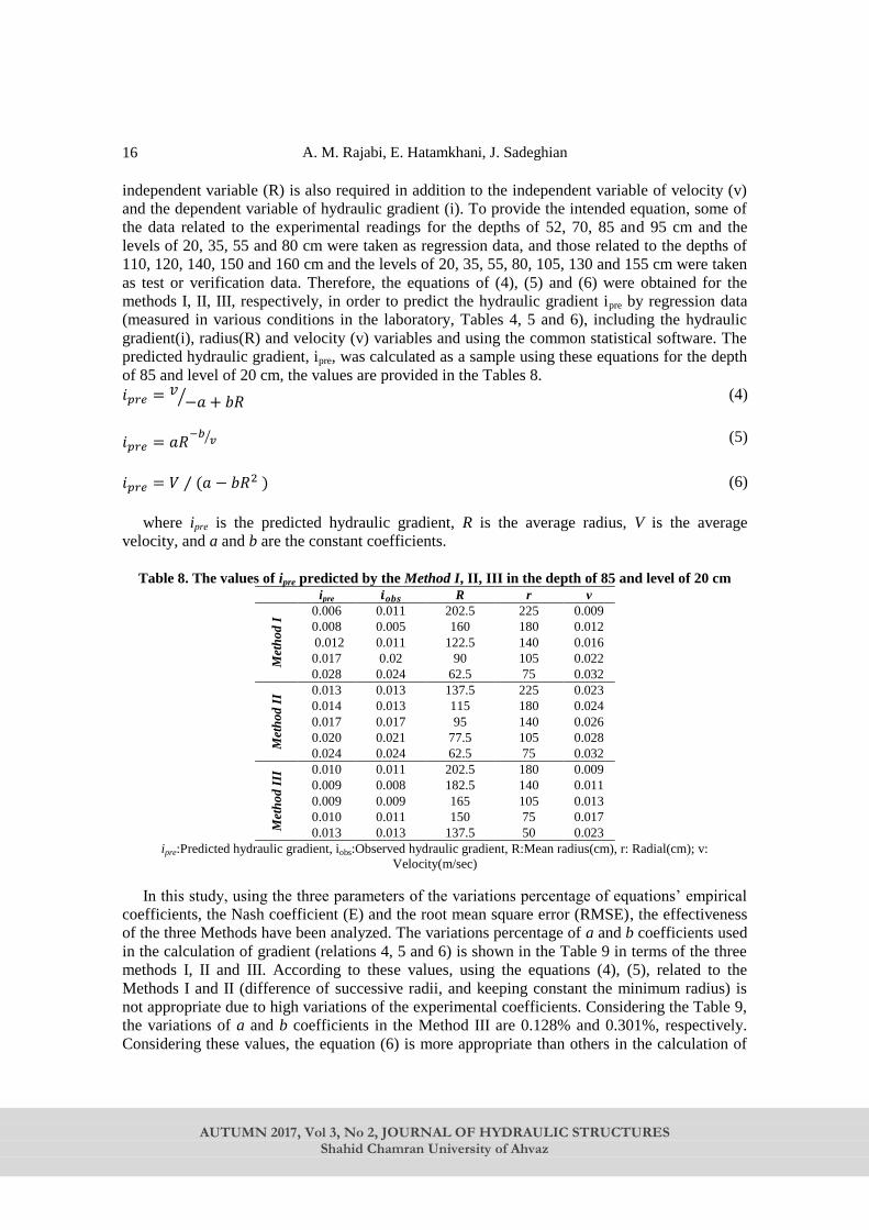
independent variable (R) is also required in addition to the independent variable of velocity (v)
and the dependent variable of hydraulic gradient (i). To provide the intended equation, some of
the data related to the experimental readings for the depths of 52, 70, 85 and 95 cm and the
levels of 20, 35, 55 and 80 cm were taken as regression data, and those related to the depths of
110, 120, 140, 150 and 160 cm and the levels of 20, 35, 55, 80, 105, 130 and 155 cm were taken
as test or verification data. Therefore, the equations of (4), (5) and (6) were obtained for the
methods I, II, III, respectively, in order to predict the hydraulic gradient ipre by regression data
(measured in various conditions in the laboratory, Tables 4, 5 and 6), including the hydraulic
gradient(i), radius(R) and velocity (v) variables and using the common statistical software. The
predicted hydraulic gradient, ipre, was calculated as a sample using these equations for the depth
of 85 and level of 20 cm, the values are provided in the Tables 8.
𝑖𝑝𝑟𝑒 = 𝑣−𝑎 + 𝑏𝑅⁄ (4)
𝑖𝑝𝑟𝑒 = 𝑎𝑅−𝑏
𝑣⁄ (5)
𝑖𝑝𝑟𝑒 = 𝑉 ⁄ (𝑎 − 𝑏𝑅2 ) (6)
where ipre is the predicted hydraulic gradient, R is the average radius, V is the average
velocity, and a and b are the constant coefficients.
Table 8. The values of ipre predicted by the Method I, II, III in the depth of 85 and level of 20 cm
v r R 𝒊𝒐𝒃𝒔 ipre
0.009 225 202.5 0.011 0.006
Met
ho
d I
0.012 180 160 0.005 0.008
0.016 140 122.5 0.011 0.012
0.022 105 90 0.02 0.017
0.032 75 62.5 0.024 0.028
0.023 225 137.5 0.013 0.013
Met
ho
d I
I
0.024 180 115 0.013 0.014
0.026 140 95 0.017 0.017
0.028 105 77.5 0.021 0.020
0.032 75 62.5 0.024 0.024
0.009 180 202.5 0.011 0.010
Met
ho
d I
II
0.011 140 182.5 0.008 0.009
0.013 105 165 0.009 0.009
0.017 75 150 0.011 0.010
0.023 50 137.5 0.013 0.013
ipre:Predicted hydraulic gradient, iobs:Observed hydraulic gradient, R:Mean radius(cm), r: Radial(cm); v:
Velocity(m/sec)
In this study, using the three parameters of the variations percentage of equations’ empirical
coefficients, the Nash coefficient (E) and the root mean square error (RMSE), the effectiveness
of the three Methods have been analyzed. The variations percentage of a and b coefficients used
in the calculation of gradient (relations 4, 5 and 6) is shown in the Table 9 in terms of the three
methods I, II and III. According to these values, using the equations (4), (5), related to the
Methods I and II (difference of successive radii, and keeping constant the minimum radius) is
not appropriate due to high variations of the experimental coefficients. Considering the Table 9,
the variations of a and b coefficients in the Method III are 0.128% and 0.301%, respectively.
Considering these values, the equation (6) is more appropriate than others in the calculation of

An experimental study on hydraulic behavior of free-surface …
AUTUMN 2017, Vol 3, No 2, JOURNAL OF HYDRAULIC STRUCTURES
Shahid Chamran University of Ahvaz
17
hydraulic gradient by keeping the maximum radius constant.
Table 9. Variation percentage of a and b coefficients in the three methods
b a Variation percentage
0.236 0.671 Method I
0.173 0.294 Method II
0.301 0.128 Method III
In this study, Nash coefficient (E) and Root Mean Square (RMS) are used to measure the
hydrological prediction ability as the equations (7) & (8).
(7)
𝐸 = 1 −∑ (𝑁𝑖(0) − 𝑁𝑖(𝑝))2𝑛
𝑖=1
∑ (𝑁𝑖(0) − 𝑁𝑚)2𝑛𝑖=1
(8) 𝑅𝑀𝑆𝐸 = √∑ (𝑁𝑖(0) − 𝑁𝑖(𝑝))2𝑛
𝑖=1
𝑛
In these equations, 𝑁𝑖(0), 𝑁𝑖(𝑝) and 𝑁𝑚 are the observed, predicted and mean values,
respectively, and n is the number of the data. The closer the E and RMSE to 1 and 0,
respectively, the more suitable the behavior of the model or equation. Table 10 shows the values
of E and RMSE to evaluate the three methods related to different depths and levels. According
to the Table 10, the values of E and RMSE related to the Method III are closer to 1 and 0,
respectively. Table 10. The values of E and RMSE in the three Methods (I, I and III)
E RMSE z Depth
(III) (II) (I) (III) (II) (I)
0.9989 0.7143 0.4762 0.0007 0.0007 0.0118 20 52
0.9993 0.4140 0.5760 0.0007 0.0013 0.0123 35 52
0.9989 0.5138 0.3759 0.0005 0.0009 0.0082 20 70
0.9971 0.2139 0.5759 0.001 0.0007 0.0093 35 70
0.9452 0.3144 0.3762 0.0219 0.0004 0.0071 55 70
0.9991 0.7145 0.4763 0.00061 0.0008 0.0949 20 85
0.95125 0.6141 0.7760 0.0005 0.0005 0.0057 35 85
0.9300 0.7137 0.8758 0.00028 0.0007 0.0041 55 85
0.9776 0.7144 0.3762 0.00057 0.0004 0.0053 80 85
0.8943 0.5142 0.8761 0.0003 0.0002 0.0044 20 95
0.9416 0.3143 0.9762 0.0005 0.0003 0.8354 35 95
0.9971 0.6141 0.5760 0.0005 0.0002 0.8372 55 95
0.9743 0.7145 0.0763 0.000629 0.0003 0.0043 80 95
D: Depth (cm); z: Water level (cm); RMSE: Root Mean Square; E: Nash Coefficient
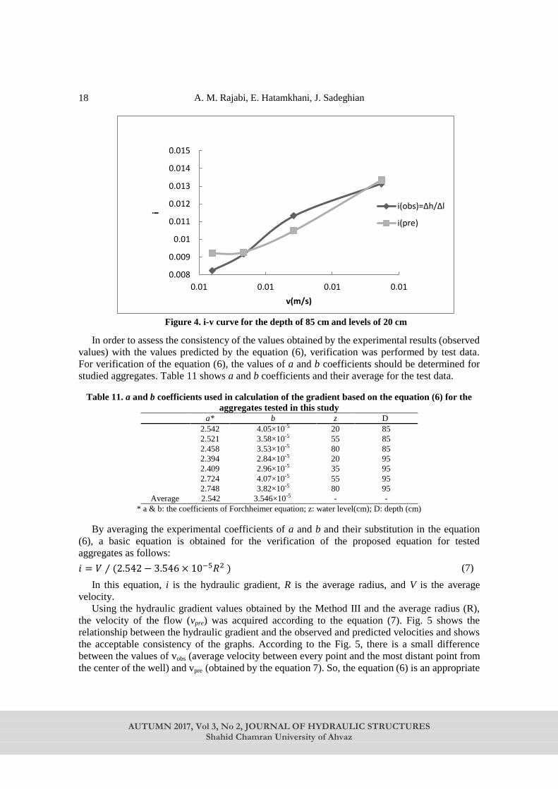
For example, the data in Table 6 for the Method III (Equation 6) is provided in Fig. 4 as a
relationship between ipre and iobs values and the average velocity. The values of RMSE and E
obtained by Table 10 are, respectively, 0.0006 and 0.9991, showing the closeness of ipre values to
iobs values using the equation (6). Then this equation would be an appropriate equation for the
description of free-surface radial flow behavior.
A. M. Rajabi, E. Hatamkhani, J. Sadeghian
AUTUMN 2017, Vol 3, No 2, JOURNAL OF HYDRAULIC STRUCTURES
Shahid Chamran University of Ahvaz
18
Figure 4. i-v curve for the depth of 85 cm and levels of 20 cm
In order to assess the consistency of the values obtained by the experimental results (observed
values) with the values predicted by the equation (6), verification was performed by test data.
For verification of the equation (6), the values of a and b coefficients should be determined for
studied aggregates. Table 11 shows a and b coefficients and their average for the test data.
Table 11. a and b coefficients used in calculation of the gradient based on the equation (6) for the
aggregates tested in this study D z b a*
85 20 4.05×10⁻⁵ 2.542
85 55 3.58×10⁻⁵ 2.521
85 80 3.53×10⁻⁵ 2.458
95 20 2.84×10⁻⁵ 2.394
95 35 2.96×10⁻⁵ 2.409
95 55 4.07×10⁻⁵ 2.724
95 80 3.82×10⁻⁵ 2.748
- - 3.546×10⁻⁵ 2.542 Average
* a & b: the coefficients of Forchheimer equation; z: water level(cm); D: depth (cm)
By averaging the experimental coefficients of a and b and their substitution in the equation
(6), a basic equation is obtained for the verification of the proposed equation for tested
aggregates as follows:
(7) 𝑖 = 𝑉 ⁄ (2.542 − 3.546 × 10⁻⁵𝑅2 )
In this equation, i is the hydraulic gradient, R is the average radius, and V is the average
velocity.
Using the hydraulic gradient values obtained by the Method III and the average radius (R),
the velocity of the flow (vpre) was acquired according to the equation (7). Fig. 5 shows the
relationship between the hydraulic gradient and the observed and predicted velocities and shows
the acceptable consistency of the graphs. According to the Fig. 5, there is a small difference
between the values of vobs (average velocity between every point and the most distant point from
the center of the well) and vpre (obtained by the equation 7). So, the equation (6) is an appropriate
0.008
0.009
0.01
0.011
0.012
0.013
0.014
0.015
0.01 0.01 0.01 0.01
i
v(m/s)
i(obs)=∆h/∆l
i(pre)

An experimental study on hydraulic behavior of free-surface …
AUTUMN 2017, Vol 3, No 2, JOURNAL OF HYDRAULIC STRUCTURES
Shahid Chamran University of Ahvaz
19
functional form for the analysis of the hydraulic behavior of the free surface radial flows.
Figure 5. i-v curve for the depth of 110 cm and the levels of 20 cm
4 Conclusions Equations of fluids in porous media are very useful in designing the rockfill dams, diversion
dams, gabions, breakwaters, and ground water reserves. The behaviors of the parallel and radial
flows are totally different. Of importance among the differences is the constant and variable
cross section of the flow in parallel and radial flows, respectively. This determines the type of
variations between the flow velocity and hydraulic gradient along the way, and also variations in
the profile of velocity-hydraulic gradient (i-v) curve. A new equation has to be developed which
is applicable for the course grained porous media due to the negative coefficient of the nonlinear
binomial Forchheimer equation in practical applications of the radial flows on the one hand, and
the invalidity of the mentioned equation for the description of the free surface radial flows in the
course grained porous media, on the other. Accordingly, in the present paper, a radial flow to the
center of a well was modeled by developing a semi cylindrical physical model. Thereafter,
different flow parameters were measured, including flow rate, hydraulic gradient, velocity, radial
distance from the center of the model and various levels. Then, choosing a series of data as
regression data, different equations were obtained for the prediction of hydraulic gradient by the
three methods of difference of successive radii, keeping constant the minimum radius and
keeping constant the maximum radius. The comparison of the attained the equations and
verification of results obtained by them was shown that the functional form of the equation
i = V ⁄ (a − bR2 ) is appropriate for the analysis of the hydraulic behavior of free surface radial
flows. This study was performed on a bed with a predetermined grain size and flow rate and in
the laboratory conditions. This phenomena is slightly different in nature than what has been
observed in the study. This study can be carried out in a porous medium with different
granulation, different flow rates and hydraulic gradients and compared to the results of this
study. Also, changing the dimensions of the physical model and therefore the boundary
conditions, can yield different results.
0.004
0.005
0.006
0.007
0.008
0.009
0.01
0.0060 0.0110 0.0160 0.0210
i
v(m/s)
v(obs)
v(pre)

A. M. Rajabi, E. Hatamkhani, J. Sadeghian
AUTUMN 2017, Vol 3, No 2, JOURNAL OF HYDRAULIC STRUCTURES
Shahid Chamran University of Ahvaz
20
5. References
1. Ahmed, N., Sunada, D.K.: Nonlinear flow in porous media. J. Hydra. Divi. ASCE. 95(6), 847-
1857 (1969)
2. Bazargan, J., Zamanisabzi, H.: Application of New Dimensionless Number for Analysis of
Laminar, Transitional and Turbulent Flow through Rock-fill Materials. Canadian Journal on
Environmental, Construction and Civil Engineering. 2(7), 2011
3. Bazargan, J., Byatt, H.: A new method to supply water from the sea through rockfill intakes.
Proceeding of 5th international conference on coasts, ports and marine structures
(ICOPMAS), October 14-17, Ramsar, Iran, PP.276-279 (2002)
4. Bazargan, J., Shoaie, M.: Non-Darcy flow analysis of rockfill materials using gradually varied
flow theory. Journal of Civil Engineering and Surveying, 44(2), 131-139 (2010)
5. Ferdos, F., Dargahi, B.: A study of turbulent flow in large-scale porous media at high
Reynolds numbers. Part I: numerical validation, Journal of Hydraulic Research. 54 (6), 663-
677 (2016 a)
6. Ferdos, F., Dargahi, B.: A study of turbulent flow in large-scale porous media at high
Reynolds numbers. Part II: flow physics, Journal of Hydraulic Research, 54 (6), 678-691
(2016 b)
7. Hansen, Garga, V.K., Townsend, D.R.: Selection and application of a one-dimensional non-
darcy flow equation for two dimensional flow through rockfill embankment. Can. Geotech. J.
33, 223-232 (1995)
8. Sadeghian, J., Khayat Kholghi, M., Horfar, A., Bazargan, J.: Comparison of Binomial and
Power Equations in Radial Non-Darcy Flows in Coarse Porous Media. JWSR Journal. 5 (1)
65- 75 (2013)
9. Li, B., Garga, V.K., Davies, M.H.: Relationship for non-Darcy flow in rockfill. J. Hydraul.
Eng., ASCE. 124(2), 206-212 (1998)
10. Mc Whorter, D.B., Sunada, D.K.: Groundwater Hydrology and hydraulics. Water Resources
Publication, Fort Collins, Colorado, USA, PP. 65-73 (1977)
11. Mc Corquodale J.A.: Finite Element Analysis of Non-Darcy Flow. Ph D Thesis, University
of Windsor, Windsor, Canada (1970).
12. Sedghi-Asl, M., Rahimi, H., Farhoudi, J., Hoorfar A., Hartmann, S.: One-Dimensional Fully
Developed Turbulent Flow through Coarse Porous Medium. Journal of Hydrologic
Engineering. 19(7), 2014.
13. Nasser, M.S.S.: Radial Non-Darcy flow through porous media. Master of Applies science
thesis, University of Windsor, Windsor, Canada (1970)
14. Reddy, N.B.: Convergence factors effect on non- uniform flow through porous media. IE(I)
Journal.CV. 86, (2006)
15. Reddy, N.B., Roma Mohan Rao, P.: Effect of convergence on nonlinear flow in porous
media.Hydr. Engrs ASCE. April 420-427 (2006)
16. Sadegian. J.: Nonlinear analysis of radial flow in coarse alluvial beds, Ph.D Thesis, College
of Agriculture, University of Tehran, Iran (2013)
17. Das, B.M, Sobhan, K.: Principles of Geotechnical Engineering, Eighth Edition, SI ,
Publisher, Global Engineering: Christopher M. Shortt; Printed in the USA (2012)
18. Thiruvengadam, M., Pradip Kumar G.N.: Validity of forchheimer equation in radial flow
through Coarse granular media. Journal of engineering mechanics, 123(7), (1997)
19. Venkataraman, P., Roma Mohan Rao, P.: Validation of Forchheimer law for flow through
porous Media with converging boundaries. J. of Hydr. Engrs. ASCE. Jan. 63-71 (2000)

An experimental study on hydraulic behavior of free-surface …
AUTUMN 2017, Vol 3, No 2, JOURNAL OF HYDRAULIC STRUCTURES
Shahid Chamran University of Ahvaz
21
20. Ward, J.C.: Turbulent flow in porous media. J. Hydra. Div. ASCE. 95 (6), 1-11 (1964)
21. Wright D.E.: Seepage Patterns Arising from Laminar, Transitional and Turbulent Flow
through Granular Media. Ph.D Thesis, University of London, UK 1958.

AUTUMN 2017, Vol 3, No 2, JOURNAL OF HYDRAULIC STRUCTURES
Shahid Chamran University of Ahvaz
Journal of Hydraulic Structures
J. Hydraul. Struct., 2017; 3(2): 22-31
DOI: 10.22055/jhs.2018.24654.1062
Three-dimensional numerical modeling of score hole in
rectangular side weir with finite volume method
Samira Ghotbi1
Azam Abdollahi2
Mehdi Azhdari Moghadam3
Abstract Local scouring in the downstream of hydraulic structures is one of the important issues in river
and hydraulic engineering, which involves a lot of costs every year, so the prediction of the rate
of scour is important in hydraulic design. Side weirs are the most important of hydraulic
structures that are used in passing flow. This study investigates the scouring due to falling jet
from side weir in downstream in side channel numerically. The simulation was done with finite
volume method. The comparison of numerical and experimental results of flow fields shows
agreement. Results show that from upstream to downstream of side weir located in side channel,
scoring is increased and the dimensions of the scour hole in the downstream of the rectangular
side weirs increase along it. In fact, at the downstream of the lower edge of side weirs in side
channel, scouring has the greatest dimensions; in particular the depth.
Keywords: Scour, Side weir, Three-dimensional Modeling, Finite volume method.
Received: 08 October 2017; Accepted: 06 November 2017
1. Introduction Side weirs are common hydraulic structures that are used to transfer water from the main
canal to the side channel, these structures are used to control flood and divert temporary flow. So
far, many studies have been conducted on the discharge coefficient ([1], to [4]) and changes in
the geometry of these side weirs ([5], to [7]) in a fixed bed. G. Michellazo, in an experimental
study investigated the effect of the moving bed in the main channel on the flow properties of
rectangular side weir. Finally, the results showed that the side weir in the moving bed for
deviating the flow is much more effective than in the fixed bed [8]. Scouring is a natural
1
Faculty of Civil Engineering, University of Sistan and Baluchestan, Zahedan, Iran,
[email protected] (Corresponding author) 2
Faculty of Civil Engineering, University of Sistan and Baluchestan, Zahedan, Iran,
Faculty of Civil Engineering, University of Sistan and Baluchestan, Zahedan, Iran,

Three-dimensional numerical modeling of score hole …
AUTUMN 2017, Vol 3, No 2, JOURNAL OF HYDRAULIC STRUCTURES
Shahid Chamran University of Ahvaz
23
phenomenon due to water flow on erosion bed’s rivers and canals. Also local scouring is part of
the morphological changes of the waterways, which is mainly due to various structures made by
human [9]. Up to now, a lot of study has carried out on the local scoring in the downstream of
the conserved bed. Farhoudi & Smith, examined the scour profiles in the downstream of
hydraulic jump and presented the scour hole according to dimensionless profiles [10].
Balachandar et al., investigated the effect of a tail water depth on scour hole development on a
loose bed of cohesion less sand material then provided diagrams for the development of the
scour hole at different times [11]. The outflow of hydraulic structures is often as a jet that may
causes significant changes in the topography of the river and surrounding these structures. It is
caused substantial damages and environmental effects. The jet with high speed creates a great
shear stress which often has a critical shear stress to start moving particles. Passing time, bed
scour increases scour depth also reduces shear stress that causes a reduction the rate of scour
[12]. With time, this leads to equilibrium a scour depth [13]. Equilibrating in the scour depth is
an approximation phenomenon [11]. Jo Jong-Song, in a 2D numerical model investigate the
local scour alteration in open channels of a tideland dike and concluded as the width of open
channel between tideland dikes decreased, due to increased flow velocity, the scoured depth
intensely increased [14]. M. Burkow, M. Griebel, investigate a 3D numerical simulation of fluid
flow and sediment transport at rectangular obstacle. Results show the typical vortex system for
the sediment transport and its interplay with shear stress and transport rates [15]. Török et al.,
offered a combined application of two bedload transport formulas that extends the application
usage. Consequently more suitable simulation results [16].
Figure1. Flow pattern of falling jet in score hole
Sediment transmission and Problems concerning its caused existence challenge in hydraulic
structures. This subject is studied by engineers and river morphologists. In recent years,
hydraulic and sediment science have progressed vastly. For the first time Shields examined the
threshold of sediment motion. He presented a diagram that is surveyed the stability of soil
channel and rivers. There are several insight for estimating the dimension of scour hole in the
downstream of hydraulic structures. Several analytical, experimental, and laboratory relationship
has been proposed to determine the depth, width and length of scour hole ([17], [18]). One of the
Relationships for estimating the depth of the scour hole in the downstream of Falling jet is
Veronese [19]:
(1)
That q is flow rate and H1 is the height of the cascade. The above relation is very simple and
just using these two parameters, the depth of the scour hole can be calculated and the effect of
0.54 0.225
11.9sd q H

S. Ghotbi, A. Abdollahi, M. Azhdari M.
AUTUMN 2017, Vol 3, No 2, JOURNAL OF HYDRAULIC STRUCTURES
Shahid Chamran University of Ahvaz
24
sediment properties is not considered. Another relationship to calculate the depth of scouring is
given that In addition to the the above parameters, also the physical properties of the sediment,
are considered [20].
(2)
g, dw and d, are Gravity acceleration, the depth of tail water depth, and the particle diameter
index respectively which, according to their suggestion, is the same as the average particle
diameter d50. According to the previews studies, Investigation of scouring in downstream of
side wires is unprecedented. Thus in this research a numerical model of scouring due to falling
jet from rectangular lateral side weir has been investigated. Although the prediction of scour
depth and the estimation of the final shape of the bed by laboratory models seems reasonable,
but from the point of view of cost and time, it is not affordable. Using a series of assumptions,
the governing equations of the flow and sediment can be simplified. In this research, a three
dimensional numerical model is used.
2. Mathematical modeling In this research, mathematical simulation of flow over the rectangular side weir and sediment
transport in the bed of side channel in downstream the side weir has been developed. For this
purpose, finite volume (VOF) method has been used for numerical solution of equations.
Rectangular cube cells grid has been used for the domain mesh generation. Selection of this grid
is because of easy to generation, the proper order and less memory need.
3. Governing equations: Sediment scouring models are sensitive to the turbulence model because the turbulence
model directly affects the viscosity. Using viscosity, the shear stress is calculated locally. Also,
for calculating the transport rate and erosion of the load, the local shear stress is used. The RNG
turbulence model is mainly recommended for scouring modeling in this software [21] that used
in this study. In the present study, following assumptions are used:
(a) An incompressible fluid (water) flows.
(b) The pressure distributed hydrostatically.
(c) Flow is shallow enough thus Vertical accelerations be neglected.
(d) The effects of wind and wave are ignored.
The governing equations for fluid flow in this study are the continuity and momentum
equations that are presented below.
Mass continuity equation:
(3)
Where VF is the volume fraction of the flow, ρ is the fluid density, R is the coefficient of the
cylindrical or Cartesian coordinates in the equation, DIFRis Disturbance phrase, and SORR
is the
mass source. u , v and w represent the velocity along x, y and z. xA ، yA
and zAEqual to the
fractions of the surface for flow along x, y and z. The first term on the right hand side of the
1
0.6 0.05 0.15
0.3 0.13.27
w
s
q H dd
g d
( ) ( ) ( ) xF x y z DIF SOR
uAV uA R vA wA R R
t x y z x

Three-dimensional numerical modeling of score hole …
AUTUMN 2017, Vol 3, No 2, JOURNAL OF HYDRAULIC STRUCTURES
Shahid Chamran University of Ahvaz
25
above equation is related to the disturbances and defined as:
( ) ( ) ( ) xDIF x y z
AR A R A A
x x y y z z x
(4)
And the second term on the right hand side of equation represents the change in density.
2
yx x SORF zvAuA uA RV wAP
Rc t x y z x
(5)
That P is the pressure and c is the velocity of the wave. The momentum equation in three
directions in three dimensions are: 2
1 1( )
y SORx y z x x x w s
F F F
A v Ru u u u PuA vA wA G f b u u u
t V x y z xV x V
(6)
1 1( )
y SORx y z y y y w s
F F F
A vu Rv v v v PuA vA wA G f b v v v
t V x y z xV y V
(7)
1 1( )SOR
x y z z z z w s
F F
Rw w w w PuA vA wA G f b w w w
t V x y z z V
(8)
xf ، yf
and zf parameters are the viscosity accelerations and xG
، yG and zG
are
Volumetric accelerations and xb ، yb
and zbare Flow drops in permeable environments.
4. Computational domain: In order to validate the numerical model in this study, the experimental results of rectangular
side weir were studied by Bagheri and Haydarpour [22], is used. The specifications of the
hydraulic structure are as follows. The main channel was designed with a length of 3 meters and
a width of 0.4 meters and a height of 35/0. The rectangular side weirs location is 1.8 meters from
the beginning of the channel. The side weirs specifications is presented in the table below. The
side channel is along the main channel with a same width to main channel. Bottom of the side
channel has been covered with aggregate materials. Sediment height at the bottom of the side
channel is 10 cm. The diameter of sediment aggregates in this study is equal to 0.005 mm and
their density is 2650 kg / m3.
Table1. Specifications of side weir [22]
(m3/s)inflow Length (cm) Height (cm)
0.042 30 15.4
Sediment characteristic parameters in the side channel are presented in table 2. The soil is
cohesion less. Table2. Specifications of sediment
Bed loading
Suspension
coeff.
Critical
shields
Bed
loading coeff. Angle (degree)
0.018 0.05 8 32
The coefficient of bed loading and bed loading in this numerical model are defined as the
sediment components. The first step in calculating the critical Shields number is to compute the

S. Ghotbi, A. Abdollahi, M. Azhdari M.
AUTUMN 2017, Vol 3, No 2, JOURNAL OF HYDRAULIC STRUCTURES
Shahid Chamran University of Ahvaz
26
dimensionless parameter*
iR.
(9)
Using the above equation, the critical Shields number is calculated from the following
equation.
(10)
5. Boundary Conditions: The boundary conditions for the walls in main and lateral channel are Wall no slip condition.
The symmetry boundary condition, for the water surface boundary, fixed velocity with the
specified head for the input channel and the continuative boundary condition for downstream
boundary is used. It is assumed that inlet flow is a fully developed flow. This assumption was
reasonable.
Figure2. scheme for computational domain and boundary conditions
6. Model Validation: Given that only at the bottom of the side weirs, i.e. in the sub-channel of sediment and there
is no deposition in the main channel, the flow conditions are precisely the same as the flow
field in the range of side weirs of laboratory without sediment models. And for validation, the
results of similar laboratory models can be used. To this purposes, Bagheri et al.'s [21]
laboratory model has been used. Therefore, it is used to confirm accuracy of flow velocity
profile on the side weir. As can be seen, the results are reasonable.
*0.52
, 2
* 3
0.10.054[1 exp( )]
10( )
icr i
i
R
R
, ,*
,
0.1( )s i f f s i
i s i
f
g dR d

Three-dimensional numerical modeling of score hole …
AUTUMN 2017, Vol 3, No 2, JOURNAL OF HYDRAULIC STRUCTURES
Shahid Chamran University of Ahvaz
27
Figure4. Comparison of the normalized velocity-length profiles obtained from the mathematical
and Bagheri et al.'s laboratory [22] model
7. Results and Discussion: Figure 5-7 shows the scour depth at the three upstream, downstream, and center points in the
channel cross-section. As you can see, the scouring rate in the downstream is increased by
moving from the top of the weirs to the end of it. This indicate increased eddy velocities during
the side weirs. The maximum scour at the lateral side of the side weir is 5.76 cm. The times are
relative and represent to the balance for scouring equilibrium.
t = 0.5 t = 1
Figure 5. Cross section of the channel at the upstream of side weir(x = 1.8 m)
0
0.2
0.4
0.6
0.8
1
1.2
1.4
1.6
0 0.2 0.4 0.6 0.8 1 1.2
Ux/
U
x/L
Experimental
Numerical

S. Ghotbi, A. Abdollahi, M. Azhdari M.
AUTUMN 2017, Vol 3, No 2, JOURNAL OF HYDRAULIC STRUCTURES
Shahid Chamran University of Ahvaz
28
Figure 6.- Cross section of the channel at the center of side weir (x = 1.95 m)
Figure 7. Channel cross section in downstream of side weir (x = 2.1 m)
Figure 8, which is related to scouring in the downstream of side weirs, Compared the
maximum depth of the scour hole in the three upstream, downstream, and center points of side
weirs. As it can be seen, at all three points in the downstream of the side weirs, the greatest
amount of scouring occurs in the initial times, and then the slope of the changes and the scouring
is reduced to equilibrium.
Figure 8. Comparison of maximum depth of the scour hole in upstream, downstream, and center
points of the side weirs
0
0.01
0.02
0.03
0.04
0.05
0.06
0.07
0 0.2 0.4 0.6 0.8 1
Time
X=1.8 m
X=1.95 m
X=2.1 m
max
imu
m d
epth
of
sco
ur
ho
le
(m)

Three-dimensional numerical modeling of score hole …
AUTUMN 2017, Vol 3, No 2, JOURNAL OF HYDRAULIC STRUCTURES
Shahid Chamran University of Ahvaz
29
As can be seen, Figure 9 shows the variation of scour along the sub channel during the
simulation. What emerges from this is that as time progresses, scour is increased and the
dimensions of the scour hole (length, width and depth) are increasing. There are also other points
around the hole that have scoured and have eroded in very small parts, due to the creating flow
of falling jet from the weir. Also, points with brown and red colors around the hole represent the
sedimentary hills caused by the sediment deposition in the downstream of weir. In fact, at these
points, the height of the bed is increasing. The negative sign in this figure indicates a decrease in
depth and scour, and a positive sign indicates an increase in the depth and formation of
sedimentary hills. Figure 10 shows the scouring pattern in the sub-channel. As can be seen, the
depth of the scour hole in the downstream of weir is higher at the lower edge than the other
points.
Figure 9. plan for scoring in lateral channel
Figure 10. score hole in downstream of side weir
As shown in Fig. 11, from the upstream to the downstream of the weir, due to the increase in
velocity, the kinetic energy is increased and has the highest value at the lower edge of the weir.
Also, over time, this amount has increased. In general, in areas where scouring occurs, the
amount of kinetic energy is higher than other areas. This figure is in agreement with previous
figures to scouring changes.

S. Ghotbi, A. Abdollahi, M. Azhdari M.
AUTUMN 2017, Vol 3, No 2, JOURNAL OF HYDRAULIC STRUCTURES
Shahid Chamran University of Ahvaz
30
Figure11. Turbulent kinetic energy in downstream of side weir in side channel
8. Conclusions The issue of sediment, its transmission and the problems due to its existence in hydraulic
structures is a serious subject studied by river engineers and morphologists. Side weirs are the
hydraulic structures used to transfer water from the main channel to the sub channel in order to
flood control and temporary flow transmission. At the downstream of these side weirs, due to
falling jet, erosion and scouring occur that results destruction in downstream and impose much
cost. Therefore, the investigation of the dimensions of the scour at the downstream of these
structures is very important and can be used in hydraulic design related to downstream
protection. The present study numerically investigated this issue with finite volume method and
RNG turbulence method. The results of simulations to scouring equilibrium indicate that the
dimensions of the scour hole in the downstream of the rectangular side weirs increase along it. In
fact, at the downstream of the lower edge of side weirs, scouring has the greatest dimensions and
in particular the depth. Also, sedimentary hills around the hole indicate the accuracy of this
result. This is due to the increase in the flow velocity over the weir from the upstream to
downstream, which increases the kinetic energy and, as a result, the shear stresses that arise at
the downstream are more than the critical shear stress of the sediment particles and consequently
erosion and scouring occur.
Three-dimensional numerical modeling of score hole …
AUTUMN 2017, Vol 3, No 2, JOURNAL OF HYDRAULIC STRUCTURES
Shahid Chamran University of Ahvaz
31
9. References 1. Swamee PK, Pathak SK, Ali MS, (1994). Side-weir analysis using elementary discharge coefficient.
Irrigation and drainage engineering, pp: 120(4):742-55.
2. Singh R, Manivannan D, Satyanarayana T, (1994). Discharge coefficient of rectangular side weirs.
Irrigation and Drainage Engineering, pp: 120(4):814-9.
3. Borghei SM, Jalili MR, Ghodsian MA, (1999). Discharge coefficient for sharp-crested side weir in
subcritical flow. Hydraulic Engineering, pp: 125(10):1051-6.
4. Ghodsian M, (2003). Supercritical flow over a rectangular side weir. Canadian Journal of Civil
Engineering, pp: 30(3):596-600.
5. Cheong HF, (1991). Discharge coefficient of lateral diversion from trapezoidal channel. Irrigation and
Drainage Engineering, pp: 117(4):461-75.
6. Emiroglu ME, Kaya N, Agaccioglu H, (2009). Discharge capacity of labyrinth side weir located on a
straight channel. Irrigation and drainage engineering, pp: 136(1):37-46.
7. Kaya N, Emiroglu ME, Agaccioglu H, (2011). Discharge coefficient of a semi-elliptical side weir in
subcritical flow. Flow Measurement and Instrumentation, pp: 22(1):25-32.
8. Michelazzo G, Minatti L, Paris E, Solari L, (2016). Side Weir Flow on a Movable Bed. Hydraulic
Engineering, pp: 142(6):04016007.
9. Hoffmans G. J. C. M, Pilarczyk K. W, (1995). Local scour downstream of hydraulic structures. Hydra.
Eng, pp: 121(4): 326-340.
10. Farhoudi J, Smith K. V. H, (1985). Local scour profiles downstream of hydraulic jump. Hydra. Res,
pp: 23(4): 343-358.
11. Balachandar R, Kells J. A, Thiessen R. J, (2000). The effect of tailwater depth on the dynamics of
local scour. Can. J. Civ. Eng, pp: 27, 138-150.
12. Kells J. A, Balachandar R, Hagel K. P, (2001). Effect of grain size on local channel scour below a
sluice gate. Can. J. Civ. Eng, pp: 28, 440-451.
13. Kurniawan, A., Altinakar, M. S. Graf, W. H. (2001). Flow pattern of an eroding jet. Proceedings of
XXIX IAHR Congress, Beijing, China.
14. Jo J. S, (2017). Numerical Simulation of Scour Depth in Open Channels of Tideland Dike. American
Journal of Naval Architecture and Marine Engineering, pp: 9(4):91-98.
15. Burkow M, Griebel M, (2015). A full three dimensional numerical simulation of the sediment
transport and the scouring at a rectangular obstacle. Preprint submitted to Elsevier.
16. Török G. T, Baranya S, Rüther N, (2017). 3D CFD Modeling of Local Scouring, Bed Armoring and
Sediment Deposition. Water, pp: 9(1):56.
17. Martins RB, (1975). Scouring of Rocky River beds by free jet spillways. Int. Water Power Dam
Constr, pp: 27(4):152-3.
18. Rajaratnam N, Mazurek K, (2003). Erosion of sand by circular impinging water jets with small
tailwater. Hydraulic Engineering, ASCE, pp: 129(3):225-229
19. Veronese A., Erosion of a bed downstream from an outlet, Colorado A & M College, Fort Collins,
United States, 1937. 20. Mason PJ, Arumugam K, (1985). Free jet scour below dams and flip buckets. Hydraulic Engineering,
pp: 111(2):220-35.
21. Brethour J, Burnham J, (2010). Modeling sediment erosion and deposition with the FLOW-3D
sedimentation & scour model. Flow Science Technical Note, FSI-10-TN85, pp: 1-22.
22. Bagheri S, Heidarpour M, (2011). Characteristics of flow over rectangular sharp-crested side weirs.
Irrigation and Drainage Engineering, pp: 138(6):541-7.

AUTUMN 2017, Vol 3, No 2, JOURNAL OF HYDRAULIC STRUCTURES
Shahid Chamran University of Ahvaz
Journal of Hydraulic Structures
J. Hydraul. Struct., 2017; 3(2):32-46
DOI: 10.22055/jhs.2018.24900.1065
Experimental Study of the Effect of Base-level fall at the
Beginning of the Bend on Reduction of Scour around a
Rectangular Bridge Pier Located in the 180 Degree Sharp Bend
Mohammad Vaghefi1
Mohammad Moghanloo2
Danesh Dehghan2
Arsalan Keshavarz2
Abstract Base-level fall in river beds occurs due to varying natural or unnatural causes. Base-level fall
causes the change in the behavior of flow at the location of drop in base-level. In such situations,
most of scour occur at the foot of the slope, and slope wall retreats in the upstream direction.
This phenomenon widens the wall of the river bank, thus leading to its destruction. The amount
of bed topography variations and scour around a rectangular bridge pier with an oblong nose
located in the 90 degree angle of a 180 degree sharp bend was studied in this work by generating
base-level fall at the beginning of the 180 degree sharp bend, and it was compared with a case
without a base-level fall. The results indicated that in the case of base-level fall at the upstream
side of the bridge pier, increase in flow depth, as well as reduction in velocity at the area around
the pier, is observed, and the maximum depth of scour hole and the volume of scour hole around
the pier respectively reduce by 73 and 97% in comparison with those in the case where no base-
level fall occurs.
Keywords: 180 degree sharp bend, base-level fall, scour, bridge pier, topography.
Received: 18 October 2017; Accepted: 25 November 2017
1. Introduction As in all the other natural phenomena, rivers tend to preserve their sustainability system.
Hence, any geometric or hydraulic change in rivers entails a dynamic response from the river in
order to restore equilibrium. Such a response is at times too widespread and uncontrollable.
Base-level drop and bed erosion in rivers result in an abrupt change in bed slope and generation
of knickpoints, all leading to base-level fall. In geomorphology, knickpoints are a part of rivers
1
Civil Engineering Department, Persian Gulf University, Bushehr, Iran. [email protected]
(Corresponding author) 2 Civil Engineering Department, Persian Gulf University, Bushehr, Iran.

Experimental Study of the Effect of Base-level fall …
AUTUMN 2017, Vol 3, No 2, JOURNAL OF HYDRAULIC STRUCTURES
Shahid Chamran University of Ahvaz
33
or channels, causing discontinuities on the slope and bed level of channels, and they occur
vertically or inclined on channel bed.
Figure 1. Inclined and vertical knickpoints (Julien, 2002)
Knickpoints make river beds unstable. River system confronts bed degradation and erosion
at the upstream, and sedimentation at the downstream sides of the knickpoint. This process
means expansion and migration of the knickpoint, damage to surrounding structures and lands,
and bed topography variations. Several studies have been conducted on bed level variations
before, a summary of which is presented in the following:
Brush and Wolman (1960) carried out an experimental study of the behavior of a drop in a
bed constituted of non-cohesive material. The generated knickpoints in these experiments
retreated from base-level fall. Consequently, the slope at the upstream side of the drop
sharpened, while the downstream slope reduced. Transported sediments settled in the form of
dunes at the downstream side of base-level fall. Holland and Pickup (1976) studied the
knickpoint transport at the layered and cohesive sedimentary bed by creating a base-level fall in
a laboratory flume. The results indicated that placing a thin sand layer through cohesive layers
reduces the retreat velocity of the knickpoint in upstream direction. Begin et al (1980) examined
knickpoint transport in upstream direction by making a base-level fall in a 15-meter-long
laboratory flume with a 1% slope. The results revealed that under constant discharge, the
velocity of knickpoint transport upstream is reduced in time. May et al. (1989) experimentally
analyzed knickpoint erosion under the influence of hydrodynamics and geology factors. Results
showed that knickpoint erosion depends on factors including knickpoint geometry, water
velocity, and the pressure developed at the downstream side of the knickpoint, so that the
occurrence of base-level fall as well as water velocity and pressure drop can help control bed
erosion at the downstream side of the knickpoint to a great extent. Garcia and Parker (1993)
conducted an experimental study of water jump resulting from a turbid flow by creating base-
level fall in a channel. The results indicated that varying the level in a turbid flow (converting a
supercritical flow into a subcritical flow due to water jump) leads to a great decrease in bed shear
stress at the downstream side of the water jump. Migeon et al. (2011) studied the effect of
changing the slope on turbid flows existing in nature by using field data. Their results
demonstrated that the hydraulic jump caused by slope reduction leads to a drop in velocity of the
turbid flow and in bed shear stress; thus the sediments of turbid flow in this zone suddenly settle.
Turmel and Locat (2012) created a base-level fall in a laboratory flume in order to examine
factors influencing the knickpoint displacement towards upstream under turbid flow conditions.
The results suggested that upstream movement of knickpoint in a turbid flow occurs as a result
of two erosive factors of turbid flow and the process of sedimentary material slippage at the
upstream side of the base-level fall area. Cantelli and Muto (2014) conducted an experimental
study on the effect of an abrupt drop at the base-level of the river on formation of knickpoints

M. Vaghefi, M. Moghanloo, D. Dehghan, A. Keshavarz
AUTUMN 2017, Vol 3, No 2, JOURNAL OF HYDRAULIC STRUCTURES
Shahid Chamran University of Ahvaz
34
migrating upstream. The drop caused numerous staircase knickpoints on the bed of the channel,
all of which retreated in upstream direction, and a hydraulic jump occurred on every stair. The
results indicated that an abrupt change in base-level led to conversion of the supercritical flow
into a subcritical flow at the downstream side of the slope, thus reducing bed shear stress of the
flow at the downstream side of the slope. Grimaud et al (2016) experimentally examined the
profile of river and knickpoint, and concluded that for a constant rate of base-level fall,
knickpoints of similar forms occur. Retreat velocity, the front slope angle, and the hole depth at
the downstream side of the knickpoint highly depend upon the structure of bed material. Also,
time intervals between knickpoint formations depend on bed thickness and rate of base-level
drop. Meandering rivers are the most common type of rivers in plan. However, a comprehensive
study is yet required to be conducted on base-level variations in a bend.
The current study experimentally addresses a method of preventing destruction of
downstream structures, and retreating erosion. In this method, the amount of local scour around
a rectangular bridge pier with an oblong nose located in the 90 degree position is examined by
dropping base level at the beginning of a 180 degree sharp bend and creating a base-level fall.
Bed topography variations, material displacement at the beginning of the bend and the sideway
banks, and the difference in the maximum scour, dimensions, and the volume of scour hole were
studied.
2. Materials and Methods Experiments were carried out in a bended channel with a 180 degree bend. Figure (2) depicts the
channel. This rectangular channel is 1 meter wide and 70 cm high at the section. The straight
upstream- and downstream-directed paths are respectively 6.5, and 5 meters long. The central
curvature radius of the bend is 2 meters. With a ratio of R/B=2, according to classification proposed
by Leschziner & Rodi (1979), this channel falls into the category of sharp bends, where R denotes
the central radius of the bend, and B the channel width. Considering the research efforts by Chiew
& Melville (1987), the standard deviation of sediment particles must be less than 1.3 in order to
preserve the effect of non-uniformity of particles on scour. Also, according to experiments
conducted by Raudkivi & Ettema (1983) aiming at prevention of ripple formation upstream, the
average diameter of the particles must not be smaller than 0.7 mm. Hence, particles with an average
diameter of 1.5 mm and standard deviation of 1.14 were employed in this laboratory. All the
experiments were conducted under inception motion conditions with a ratio of flow velocity to
critical velocity (U/Uc) equal to 0.97.According to Oliveto & Hager (2002), in order to prevent
roughness effects, the water depth must exceed 20 mm; therefore, a discharge capacity of 70 liters
per second and a depth of 18 cm were selected for conducting the experiments.
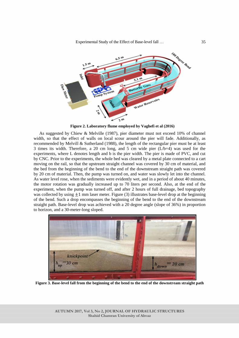
Experimental Study of the Effect of Base-level fall …
AUTUMN 2017, Vol 3, No 2, JOURNAL OF HYDRAULIC STRUCTURES
Shahid Chamran University of Ahvaz
35
Figure 2. Laboratory flume employed by Vaghefi et al (2016)
As suggested by Chiew & Melville (1987), pier diameter must not exceed 10% of channel
width, so that the effect of walls on local scour around the pier will fade. Additionally, as
recommended by Melvill & Sutherland (1988), the length of the rectangular pier must be at least
3 times its width. Therefore, a 20 cm long, and 5 cm wide pier (L/b=4) was used for the
experiments, where L denotes length and b is the pier width. The pier is made of PVC, and cut
by CNC. Prior to the experiments, the whole bed was cleared by a metal plate connected to a cart
moving on the rail, so that the upstream straight channel was covered by 30 cm of material, and
the bed from the beginning of the bend to the end of the downstream straight path was covered
by 20 cm of material. Then, the pump was turned on, and water was slowly let into the channel.
As water level rose, when the sediments were evidently wet, and in a period of about 40 minutes,
the motor rotation was gradually increased up to 70 liters per second. Also, at the end of the
experiment, when the pump was turned off, and after 2 hours of full drainage, bed topography
was collected by using ±1 mm laser meter. Figure (3) illustrates base-level drop at the beginning
of the bend. Such a drop encompasses the beginning of the bend to the end of the downstream
straight path. Base-level drop was achieved with a 20 degree angle (slope of 36%) in proportion
to horizon, and a 30-meter-long sloped.
Figure 3. Base-level fall from the beginning of the bend to the end of the downstream straight path
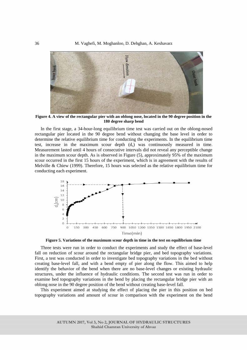
M. Vaghefi, M. Moghanloo, D. Dehghan, A. Keshavarz
AUTUMN 2017, Vol 3, No 2, JOURNAL OF HYDRAULIC STRUCTURES
Shahid Chamran University of Ahvaz
36
Figure 4. A view of the rectangular pier with an oblong nose, located in the 90 degree position in the
180 degree sharp bend
In the first stage, a 34-hour-long equilibrium time test was carried out on the oblong-nosed
rectangular pier located in the 90 degree bend without changing the base level in order to
determine the relative equilibrium time for conducting the experiments. In the equilibrium time
test, increase in the maximum scour depth (ds) was continuously measured in time.
Measurement lasted until 4 hours of consecutive intervals did not reveal any perceptible change
in the maximum scour depth. As is observed in Figure (5), approximately 95% of the maximum
scour occurred in the first 15 hours of the experiment, which is in agreement with the results of
Melville & Chiew (1999). Therefore, 15 hours was selected as the relative equilibrium time for
conducting each experiment.
Figure 5. Variations of the maximum scour depth in time in the test on equilibrium time
Three tests were run in order to conduct the experiments and study the effect of base-level
fall on reduction of scour around the rectangular bridge pier, and bed topography variations.
First, a test was conducted in order to investigate bed topography variations in the bed without
creating base-level fall, and with a bend empty of pier along the flow. This aimed to help
identify the behavior of the bend when there are no base-level changes or existing hydraulic
structures, under the influence of hydraulic conditions. The second test was run in order to
examine bed topography variations in the bend by placing the rectangular bridge pier with an
oblong nose in the 90 degree position of the bend without creating base-level fall.
This experiment aimed at studying the effect of placing the pier in this position on bed
topography variations and amount of scour in comparison with the experiment on the bend

Experimental Study of the Effect of Base-level fall …
AUTUMN 2017, Vol 3, No 2, JOURNAL OF HYDRAULIC STRUCTURES
Shahid Chamran University of Ahvaz
37
without a pier. The third test was conducted with the aim of examining the effect of drop on bed
topography of the bend and scour around the rectangular bridge pier. The results are addressed in
the following section.
3. Results and Discussion After determination of the relative equilibrium time, the experiment was conducted in an
empty bend without a pier in order to provide a better understanding of flow behavior and bed
topography variations in the bend. Bed topography after equilibrium time is presented in Figure
(6). As is evident in the figure, bed topography in the bend is accompanied by sedimentation at
the inner bank as well as erosion at the outer bank, due to formation of helical flows.
Figure 6. Bed topography variations in the case of empty bend (without a pier)
As noted in Figure (6), sedimentation in the vicinity of the inner wall began at the 35 degree
and lasted until the 145 degree angle. The maximum sedimentation has occurred for 8.7 cm
(equivalent to 0.087 times the channel width) in the 65 degree position. Further, the scour began
at the 35 degree angle and lasted until the 95 degree angle, as is observed in the figure. The
maximum scour also occurred for 4.2 cm (equivalent to 0.042 times the channel width) at the 65
degree angle. Results refer to the maximum degree of helical flow strengths at the 60 to 70
degree interval of the bend. Then, a better understanding of the effect of base-level fall in the
presence of the pier on bed topography of the bend is achieved by conducting the following
experiments and comparing their topographies with the experiment on the bend without a pier.
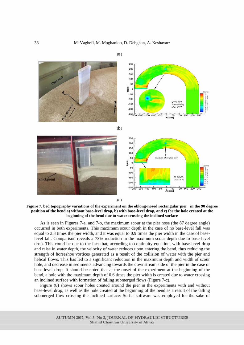
M. Vaghefi, M. Moghanloo, D. Dehghan, A. Keshavarz
AUTUMN 2017, Vol 3, No 2, JOURNAL OF HYDRAULIC STRUCTURES
Shahid Chamran University of Ahvaz
38
(a)
(b)
(c)
Figure 7. bed topography variations of the experiment on the oblong-nosed rectangular pier in the 90 degree
position of the bend a) without base-level drop, b) with base-level drop, and c) for the hole created at the
beginning of the bend due to water crossing the inclined surface
As is seen in Figures 7-a, and 7-b, the maximum scour at the pier nose (the 87 degree angle)
occurred in both experiments. This maximum scour depth in the case of no base-level fall was
equal to 3.3 times the pier width, and it was equal to 0.9 times the pier width in the case of base-
level fall. Comparison reveals a 73% reduction in the maximum scour depth due to base-level
drop. This could be due to the fact that, according to continuity equation, with base-level drop
and raise in water depth, the velocity of water reduces upon entering the bend, thus reducing the
strength of horseshoe vortices generated as a result of the collision of water with the pier and
helical flows. This has led to a significant reduction in the maximum depth and width of scour
hole, and decrease in sediments advancing towards the downstream side of the pier in the case of
base-level drop. It should be noted that at the onset of the experiment at the beginning of the
bend, a hole with the maximum depth of 0.6 times the pier width is created due to water crossing
an inclined surface with formation of falling submerged flows (Figure 7-c).
Figure (8) shows scour holes created around the pier in the experiments with and without
base-level drop, as well as the hole created at the beginning of the bend as a result of the falling
submerged flow crossing the inclined surface. Surfer software was employed for the sake of

Experimental Study of the Effect of Base-level fall …
AUTUMN 2017, Vol 3, No 2, JOURNAL OF HYDRAULIC STRUCTURES
Shahid Chamran University of Ahvaz
39
more precise calculations in measuring the volume of the hole, and drawing the figures. As
presented in Figures 8-a and 8-b, the volume of the hole created around the pier in the case of no
base-level drop and in the case of base-level drop, is respectively around 28750 and 750 𝑐𝑚3,
equal to 230 and 6 times the third power of the pier width. Also, according to Figure 8-c, due to
falling submerged flow crossing the knick point and the inclined surface, a wide hole of
3500𝑐𝑚3, equal to 28 times the third power of the pier width, is formed at the beginning of the
bend.
Figure (9) presents an instance of cross sections along the bend. Figure 9-a presents
sedimentation in the vicinity of the inner bank in the case of empty bend (without a pier), and the
case without base-level fall. This sedimentation may be due to the effect of the onset of the bend
and change in flow conditions under the influence of the sharp bend. Also, in the case of base-
level fall, because the base-level fall created at the beginning of the bend extended all through
the channel width, the width of the created hole in this area occupied 100% of the channel width,
forming a wide hole. Figure 9-b depicts a transverse profile of the channel at a distance equal to
17 times the pier depth in the upstream direction (the 65 degree position). As is observed, in the
cases of the bend without a pier, and no base-level fall, sedimentation in the vicinity of the inner
bank is respectively 1.65 and 1.15 times the pier depth, the fact which is due to the effect of the
secondary flows, their interaction with longitudinal flows, and formation of helical flows in the
bend. The maximum scour in this section occurs in the case of the bend without a pier. This
scour is 0.84 times the pier width, and occurs at a distance of 0.4 times the channel width from
the inner bank. Also, the bed in this section undergoes little change in the case of base-level fall.
Figure 9-c, the cross section is at a distance of 3 times the pier width towards the upstream side
of the pier. This section undergoes the maximum sedimentation in the case of empty bend. Such
sedimentation occurs at a distance of 0.05 times the channel width from the inner bank, at a
height of 0.38 times the pier width. The maximum scour in this section occurs in the case of no
base-level fall at a distance of 0.52 times the channel width from the inner bank at a depth of
2.68 times the pier width. This scour is a result of proximity to the pier, and presence of
horseshoe vortices. This section also undergoes little change in the case of base-level fall. As
provided in Figure 9-d, the scour hole, created at the pier nose, has occupied 60% of channel
width in the case of no base-level fall. However, after creating a base-level fall, the created hole
has occupied only 8% of channel width. Then it can be stated that base-level fall has led to 87%
decrease in the width of scour hole. The maximum scour depth in the cases with and without a
base-level drop is respectively 16.6 and 4.5 cm, equal to 3.32 and 0.9 times the pier width, i.e. a
73% reduction in the maximum scour depth due to base-level drop. The maximum sedimentation
of this section occurs for the empty bend, equal to the pier width at a distance of 0.05 times the
channel width from the inner bank.

M. Vaghefi, M. Moghanloo, D. Dehghan, A. Keshavarz
AUTUMN 2017, Vol 3, No 2, JOURNAL OF HYDRAULIC STRUCTURES
Shahid Chamran University of Ahvaz
40
(a)
(b)
(c)
Figure 8. Scour holes created a) around the bridge pier in the case of no base-level drop, b) around
the bridge pier in the case of base-level drop, and c) at the beginning of the bend in the case of base-
level drop
As is evident in Figure 9-e, sediments transported from the pier nose by horseshoe vortices
pile up at a distance of 3 times the pier width at the downstream side with a height of 0.16 times
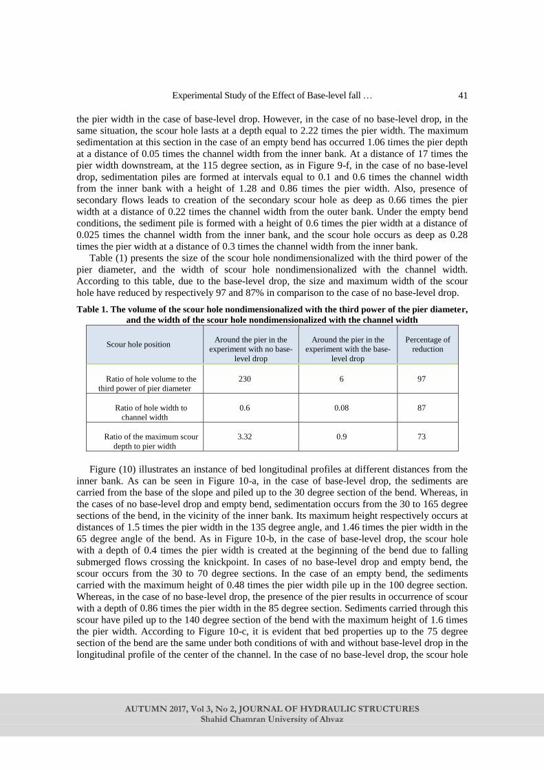
Experimental Study of the Effect of Base-level fall …
AUTUMN 2017, Vol 3, No 2, JOURNAL OF HYDRAULIC STRUCTURES
Shahid Chamran University of Ahvaz
41
the pier width in the case of base-level drop. However, in the case of no base-level drop, in the
same situation, the scour hole lasts at a depth equal to 2.22 times the pier width. The maximum
sedimentation at this section in the case of an empty bend has occurred 1.06 times the pier depth
at a distance of 0.05 times the channel width from the inner bank. At a distance of 17 times the
pier width downstream, at the 115 degree section, as in Figure 9-f, in the case of no base-level
drop, sedimentation piles are formed at intervals equal to 0.1 and 0.6 times the channel width
from the inner bank with a height of 1.28 and 0.86 times the pier width. Also, presence of
secondary flows leads to creation of the secondary scour hole as deep as 0.66 times the pier
width at a distance of 0.22 times the channel width from the outer bank. Under the empty bend
conditions, the sediment pile is formed with a height of 0.6 times the pier width at a distance of
0.025 times the channel width from the inner bank, and the scour hole occurs as deep as 0.28
times the pier width at a distance of 0.3 times the channel width from the inner bank.
Table (1) presents the size of the scour hole nondimensionalized with the third power of the
pier diameter, and the width of scour hole nondimensionalized with the channel width.
According to this table, due to the base-level drop, the size and maximum width of the scour
hole have reduced by respectively 97 and 87% in comparison to the case of no base-level drop.
Table 1. The volume of the scour hole nondimensionalized with the third power of the pier diameter,
and the width of the scour hole nondimensionalized with the channel width
Scour hole position
Around the pier in the
experiment with no base-
level drop
Around the pier in the
experiment with the base-
level drop
Percentage of
reduction
Ratio of hole volume to the
third power of pier diameter
230 6 97
Ratio of hole width to
channel width
0.6 0.08 87
Ratio of the maximum scour
depth to pier width
3.32 0.9 73
Figure (10) illustrates an instance of bed longitudinal profiles at different distances from the
inner bank. As can be seen in Figure 10-a, in the case of base-level drop, the sediments are
carried from the base of the slope and piled up to the 30 degree section of the bend. Whereas, in
the cases of no base-level drop and empty bend, sedimentation occurs from the 30 to 165 degree
sections of the bend, in the vicinity of the inner bank. Its maximum height respectively occurs at
distances of 1.5 times the pier width in the 135 degree angle, and 1.46 times the pier width in the
65 degree angle of the bend. As in Figure 10-b, in the case of base-level drop, the scour hole
with a depth of 0.4 times the pier width is created at the beginning of the bend due to falling
submerged flows crossing the knickpoint. In cases of no base-level drop and empty bend, the
scour occurs from the 30 to 70 degree sections. In the case of an empty bend, the sediments
carried with the maximum height of 0.48 times the pier width pile up in the 100 degree section.
Whereas, in the case of no base-level drop, the presence of the pier results in occurrence of scour
with a depth of 0.86 times the pier width in the 85 degree section. Sediments carried through this
scour have piled up to the 140 degree section of the bend with the maximum height of 1.6 times
the pier width. According to Figure 10-c, it is evident that bed properties up to the 75 degree
section of the bend are the same under both conditions of with and without base-level drop in the
longitudinal profile of the center of the channel. In the case of no base-level drop, the scour hole
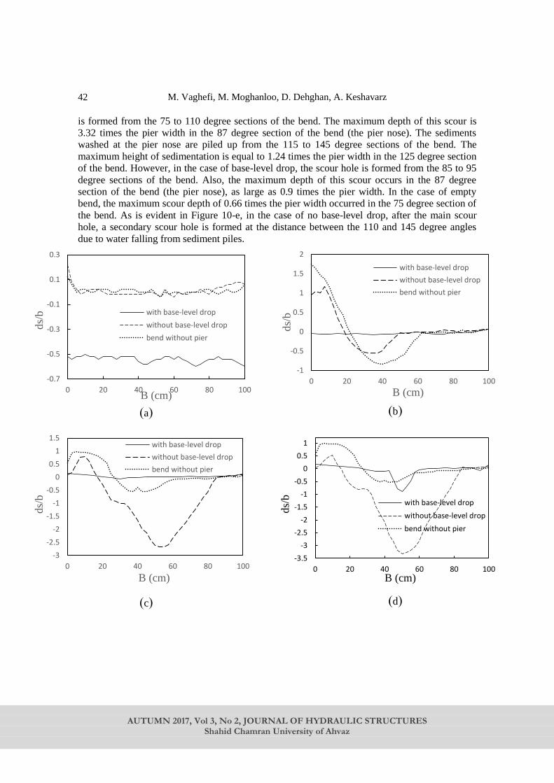
M. Vaghefi, M. Moghanloo, D. Dehghan, A. Keshavarz
AUTUMN 2017, Vol 3, No 2, JOURNAL OF HYDRAULIC STRUCTURES
Shahid Chamran University of Ahvaz
42
is formed from the 75 to 110 degree sections of the bend. The maximum depth of this scour is
3.32 times the pier width in the 87 degree section of the bend (the pier nose). The sediments
washed at the pier nose are piled up from the 115 to 145 degree sections of the bend. The
maximum height of sedimentation is equal to 1.24 times the pier width in the 125 degree section
of the bend. However, in the case of base-level drop, the scour hole is formed from the 85 to 95
degree sections of the bend. Also, the maximum depth of this scour occurs in the 87 degree
section of the bend (the pier nose), as large as 0.9 times the pier width. In the case of empty
bend, the maximum scour depth of 0.66 times the pier width occurred in the 75 degree section of
the bend. As is evident in Figure 10-e, in the case of no base-level drop, after the main scour
hole, a secondary scour hole is formed at the distance between the 110 and 145 degree angles
due to water falling from sediment piles.
(b)
(a)
(d)
(c)
-1
-0.5
0
0.5
1
1.5
2
0 20 40 60 80 100
ds/
b
B (cm)
with base-level drop
without base-level drop
bend without pier
-0.7
-0.5
-0.3
-0.1
0.1
0.3
0 20 40 60 80 100
ds/
b
B (cm)
with base-level drop
without base-level drop
bend without pier
-3.5
-3
-2.5
-2
-1.5
-1
-0.5
0
0.5
1
0 20 40 60 80 100
ds/
b
B (cm)
with base-level drop
without base-level drop
bend without pier
-3
-2.5
-2
-1.5
-1
-0.5
0
0.5
1
1.5
0 20 40 60 80 100
ds/
b
B (cm)
with base-level drop
without base-level drop
bend without pier

Experimental Study of the Effect of Base-level fall …
AUTUMN 2017, Vol 3, No 2, JOURNAL OF HYDRAULIC STRUCTURES
Shahid Chamran University of Ahvaz
43
(f) (e)
Figure 9. cross sections of a) the beginning of the bend, b) 17 times the pier width at the upstream side of the pier (65
degrees), c) 3 times the pier width at the upstream side of the pier (85 degrees), d) the pier nose, e) 3 times the pier width at
the downstream side of the pier (95 degrees), and f) 17 times the pier width at the downstream side of the pier (115
degrees)
(a)
(b)
-1
-0.5
0
0.5
1
1.5
0 20 40 60 80 100
ds/
b
B (cm)
with base-level drop
without base-level drop
bend without pier-2.5
-2
-1.5
-1
-0.5
0
0.5
1
1.5
0 20 40 60 80 100
ds/
b
B (cm)
with base-level drop
without base-level drop
bend without pier
-0.5
-0.1
0.3
0.7
1.1
1.5
1.9
0 20 40 60 80 100 120 140 160 180
ds/
b
Ɵ ( deg)
with base-level drop without base-level drop bend without pier
-1
0
1
2
0 20 40 60 80 100 120 140 160 180
ds/
b
Ɵ ( deg)
with base-level drop without base-level drop bend without pier

M. Vaghefi, M. Moghanloo, D. Dehghan, A. Keshavarz
AUTUMN 2017, Vol 3, No 2, JOURNAL OF HYDRAULIC STRUCTURES
Shahid Chamran University of Ahvaz
44
(c)
(d)
(e)
Figure 10. longitudinal sections at distances of a) 5, b) 25, c) 50, d) 75, and e) 95% of the channel
width from the inner bank
The maximum depth of the secondary scour hole, equal to 0.6 times the pier width, occurred
in the 115 degree section. In the case of base-level drop at the beginning of the bend, a scour
hole is created with the maximum depth of 0.56 times the pier width. In addition, the sediment
pile with a height of 0.2 times the pier width is formed in the 7 degree section of the bend. In the
case of empty bend, the bed variations along the bend are insignificant. According to Figure 10-
d, in the case of no base-level drop, a scour hole with the maximum depth of 0.36 times the pier
width is created in the 130 degree section of the bend, in the vicinity of the outer bank, under the
influence of the secondary flows, and their interaction with the longitudinal flow and formation
of a helical flow. In the case of base-level drop at the beginning of the bend, a scour hole has
occurred with a depth of 0.38 times the pier width, and bed variations after this scour hole are
insignificant to the end of the bend. Also, there have been few changes in the case of empty
bend.
-3.5-3
-2.5-2
-1.5-1
-0.50
0.51
1.5
0 20 40 60 80 100 120 140 160 180
ds/
b
Ɵ ( deg)
with base-level drop without base-level drop bend without pier
-1.2-1
-0.8-0.6-0.4-0.2
00.20.4
0 20 40 60 80 100 120 140 160 180
ds/
b
Ɵ ( deg)
with base-level drop without base-level drop bend without pier
-0.5
-0.3
-0.1
0.1
0.3
0 20 40 60 80 100 120 140 160 180
ds/
b
Ɵ ( deg)
with base-level drop without base-level drop bend without pier

Experimental Study of the Effect of Base-level fall …
AUTUMN 2017, Vol 3, No 2, JOURNAL OF HYDRAULIC STRUCTURES
Shahid Chamran University of Ahvaz
45
4. Conclusion This paper addressed the effect of base-level fall on scour around a rectangular bridge pier
located in the 90 degree angle of a 180 degree sharp bend. The most important findings are as
follows:
The maximum scour occurred for 16.6 cm, equal to 3.32 times the pier width at the pier nose
after installation of the pier in the intended position. However, with the position of the pier, after
applying base-level fall, the maximum scour depth occurred for 4.5 cm, equal to 0.9 times the
pier width, the fact which indicates a 73% reduction in the scour hole around the pier. In both
cases, the maximum scour depth occurred at the nose of the pier. After creating a base-level
drop, the volume of scour hole around the pier reduced by 97%, and a wide scour hole with a
size of 28 times the third power of the pier width, and the maximum depth of 0.6 times the pier
width formed at the downstream side of the slope.
5. Reference 1. Begin, Z. E. B., Schumm, S. A. and Meyer, D. F. (1980). "Knickpoint migration due to base
level lowering." Journal of the Waterway, Port, Coastal and Ocean Division, 106(3), 369-
388.
2. Brush, L.M. and Wolman, M.G. (1960 " (. Knickpoint behavior in non-cohesive material: A
laboratory study." Geological Society of America Bulletin, 71: 59-74.
3. Cantelli, A. and Muto T. (2014). "Multiple knickpoints in an alluvial river generated by a
single instantaneous drop in base level: experimental investigation." Earth Surf. Dynam, 2:
271–278.
4. Chiew, Y.M. and Melville, B.W. (1987). "Local scour around bridge piers." Journal of
Hydraulic Research, 25 (1), 15–26.
5. Garcia, M. H. and G. Parker. )1993(."Experimental on the entailment of sediment into
suspention by a dense bottom current." J. Geophys.Res. (Oceans) 98:4793-4807.
6. Grimaud, J.L., Paola1, C. and Voller, V. (2016). "Experimental migration of knickpoints:
influence of style of base-level fall and bed lithology." Earth Surf. Dynam, 4: 11–23.
7. Holland, W.N. and Pickup, G. (1976). "Flume study of knickpoint development in stratified
sediment." Geological Society of America Bulletin, 87: 76-82.
8. Julien, P. Y. (2002). "River mechanics." Cambridge University Press.
9. Leschziner, M. A. and Rodi, W. (1979). "Calculation of strongly curved open channel flow."
Journal of the Hydraulics Division, 105 (10), 1297–1314.
10. May, J.H. (1989). "Report 4: Geologic and hydrodynamic controls on the mechanics of
knickpoint migration." U.S. Army Engineer Waterways Experiment Station, Vicksburg, MS.
11. Melville, B.W. and Chiew, Y.M., (1999), "Time Scale for Local Scour Depth at Bridge
Piers." Journal of Hydraulic Engineering, ASCE, Vol.125, No.1, 59-65.
12. Melville B. W. and Sutherland A. J. (1988). "Design method for local scour at bridge piers."
American Society of Civil Engineering. Journal of the Hydraulics Division, Vol. 114, No. 10,
pp. 1210–1225.
13. Migeon, S., T. Mulder., B. Savoye. and F. Sage. (2011). "Hydrodynamic processes, velocity
structure and stratification in natural turbidity currents: results inferred from field data in the
turbidite system." J. Sedimen Geo. 245:48-62.
14. Oliveto, G. and Hager, W.H., (2002). "Temporal evolution of clear-water pier and abutment
scour." Journal of Hydraulic Engineering, 128 (9), 811–820.
15. Raudkivi, A.J. and Ettema, R., (1983). "Clear-water scour at cylindrical piers." Journal of
Hydraulic Engineering, 109 (3), 338–350.

M. Vaghefi, M. Moghanloo, D. Dehghan, A. Keshavarz
AUTUMN 2017, Vol 3, No 2, JOURNAL OF HYDRAULIC STRUCTURES
Shahid Chamran University of Ahvaz
46
16. Turmel, D., Locat, J. and Parker, G. (2012). "Upstream migration of knickpoints:
geotechnical considerations." In Submarine Mass Movements and Their Consequences (pp.
123-132).
17. Vaghefi, M., Akbari, M. and Fiouz, A. R. (2016). "An experimental study of mean and
turbulent flow in a 180 degree sharp open channel bend: Secondary flow and bed shear
stress." KSCE Journal of Civil Engineering, 20(4), 1582-1593.

AUTUMN 2017, Vol 3, No 2, JOURNAL OF HYDRAULIC STRUCTURES
Shahid Chamran University of Ahvaz
Journal of Hydraulic Structures
J. Hydraul. Struct., 2017; 3(2):47-61
DOI: 10.22055/jhs.2017.13490
Developing Optimal Operating Reservoir Rule-curves in
Drought Periods
Soroosh Alahdin1
Hamid Reza Ghafouri2
Abstract In this study, a simulation-optimization model is developed for deriving operational rule-curves
in drought periods. To each reservoir, two rule-curves with adjustable monthly levels are
introduced dividing the reservoir capacity into three zones between the normal water level and
minimum operation level. To each zone of the reservoir and for each month of the year a
hedging coefficient is introduced that determines the release from the reservoir. Accordingly, an
optimization problem is developed in which the objective is the minimization of water demands
deficits in drought and the decision variables are the rule-curves levels and hedging coefficients.
For optimization, a genetic algorithm equipped with a self-adaptive constraint handling strategy
is used. To evaluate the objective function and constraints violations, the flexible and widely-
used WEAP (Water Evaluation and Planning) simulation model is exploited and coupled with
the optimization solver. The model is then applied to the Zohreh three-reservoir system in the
southwest of Iran and compared to the Standard Operation Policy (SOP). According to the
sustainability indices for the system operated in drought, the obtained operating rule-curves are
found significantly superior to the SOP. As a result of applying the rule-curves, the modified
shortage index (MSI) and vulnerability (extent) of the system are respectively improved by 22%
and 28% compared to the SOP. Consequently, the developed policy application resulted in
longer periods of deficit (but less severe) as shown by decrease in reliability (5%) and resilience
(40%) indices.
Keywords: Operating policy, Rule-Curve, Sustainability Indices, Optimization Model, Hedging.
Received: 09 August 2017; Accepted: 20 November 2017
1 Ph.D. Candidate, Department of Civil Engineering, Engineering Faculty, Shahid Chamran University of
Ahvaz, Ahvaz, Iran, [email protected] (Corresponding author) 2 Professor, Department of Civil Engineering, Engineering Faculty, Shahid Chamran University of Ahvaz,
Ahvaz, Iran.

S. Alahdin, H.R. Ghafouri
AUTUMN 2017, Vol 3, No 2, JOURNAL OF HYDRAULIC STRUCTURES
Shahid Chamran University of Ahvaz
48
1. Introduction Handling the operational challenges has been always a serious concern for reservoirs
operators, but when a water resources system is suffering from water scarcity, demands are more
strongly competing for water and the system operation becomes even more complicated and
challenging.
Application of simulation and optimization models has shown great advances in planning and
management of water resources problems. Currently, there are several softwares like HEC3,
HEC5, HEC-ResSim, MIKEBASIN, RIBASIM, WATHNET, OASIS, ARSP, CalSim,
RiverWare, MODSIM, WRAP, SWD SUPER and WEAP that can simulate operation of a
reservoir system with its all components in details. A simulation model can evaluate the system
performance for any decision on the reservoirs releases and operations over a certain time period
and return the values of objective functions and constraint violations introduced to the system.
A reservoir system is operated following prescriptions on the system releases as a function of
time and available water. These prescriptions or more precisely rule-curves are traditionally
derived through intensive simulation techniques [1], but to derive optimum operating ones for a
multi-reservoir system, it is required to develop and solve optimization models. The optimization
systematically changes the operational parameters and the simulation model evaluates the effects
of each change on the system operation over a long period. This process continues until the best
feasible performance of the reservoir system is achieved. This is the main skeleton of every
simulation-optimization model that has recently become very popular and well-developed for
solving a variety of water resources problems. In this context, many researchers have tried to
cope with the challenges associated with the operation of reservoir systems in arid and semi-arid
areas as well as during drought periods. The existing approaches are different in concept ranging
from simplified rules of thumb to sophisticated model-based operating rules.
To minimize the impacts of a drought event, water is stored in the system for future even if
enough water exists to satisfy the current demands. The purpose of a hedging decision in a
reservoir operation is to lessen the burden of water scarcity in the future by distributing the
demands' deficits over an extended period of operation. In general, hedging rules can be
categorized into two main groups of continuous and discrete methods. Through the continuous
approach, the decisions on the amount of water to be rationed are mathematically represented by
a linear, nonlinear or fuzzy function [2-13]. Whereas, in the discrete methods the decisions are
made based on the discrete representation of the reservoir and water resources conditions [1, 14-
17]. Many investigations with the aid of simulation and optimization models were published to
extend and modify these approaches. These studies put forth and answered two key questions of,
"when to start rationing" and "how much rationing". However, this issue is highly case-
dependentandneedsathoughtfulinsightintothesystem’sobjectives,limitations,hydrologyand
other specifications.
An important concern in deriving hedging rules is the employment of proper solvers. The
applied methods are the mixed integer programming [1-2, 14-15], dynamic programming [10],
Markov Model [6, 7] and recently, heuristic nature-inspired algorithms [8-9, 11-12, 16-18]. For
the sake of dimensionality problems associated with the large-scale multi-reservoir systems,
some investigations were inevitably restricted to single-reservoir case studies or short-term time-
series [2-10, 14-15, 19].
Some studies were carried out based on surrogate simulation models rather than simulating
the system with all details. For example, to make the process of simulation-optimization more
efficient Dariane et al., [5], trained and substituted an artificial neural network for the system
simulation and Guo et al., [16], used an equivalent reservoir for a multi-reservoir system and

Developing Optimal Operating Reservoir Rule-curves in Drought Periods
AUTUMN 2017, Vol 3, No 2, JOURNAL OF HYDRAULIC STRUCTURES
Shahid Chamran University of Ahvaz
49
assumed constant weighting factors for different types of water supplies. However, issues like
the interaction between the reservoirs and other components of the system as well as the role of
long-term data encompassing different hydrological conditions are very significant in deriving
the system operating rules. Paying attention to these concerns, Taghian et al., [17], developed a
comprehensive long-term simulation model based on the ARSP for a three-reservoir system
facing with severe droughts. All water demands were also simulated in the model using the
network flow scheme. They proposed a discrete hedging rule by hybridizing a genetic algorithm
for hedging optimization and a linear programming model for allocation water to downstream
demands. In this context, the present study aims at developing a complete simulation-
optimization model for multi-reservoir systems in drought periods with some modifications. The
powerful, comprehensive and easy-to-use simulation software, WEAP is used to serve as
objective function and constraint values provider. Then, the problem is formulated as a
constrained nonlinear optimization problem and is solved using a self-adaptive Genetic
Algorithm (GA). The model is applied to a three-reservoir case study in Iran, and the results are
discussed and compared with those obtained by the SOP.
2. Case study and problem statement As a case study, drought-stricken Zohreh river system located in the south-western of Iran
with an area of 15460 squared kilometer is studied. The schematic of the system is shown in
Figure 1. The system comprises of three reservoirs, eight input stream flows, thirteen irrigation
networks, three public demands and two minimum flows. The conservation storage volumes for
Kosar, Chamshir, and Kheirabad reservoirs are respectively, 418, 1862, and 105 million cubic
meters (mcm) as presented in Table 1 in details.
Table 1. Properties of hydropower plants
Properties of dam Chamshir Kosar Kheirabad
Normal level (meter above sea level) 598 625 259.6
Minimum level of operation (meter
above sea level) 543.7 580 238
Volume storage in min. level (mcm) 454.5 74.2 0.93
Volume storage in normal level (mcm) 2316.7 492.8 106.3
Installed capacity (Mega Watt) 165 - 2.5
Plant factor (%) 25 - -
Plant efficiency (%) 91 - 85
Maximum turbine flow (cms) 144.4 - 7.26

S. Alahdin, H.R. Ghafouri
AUTUMN 2017, Vol 3, No 2, JOURNAL OF HYDRAULIC STRUCTURES
Shahid Chamran University of Ahvaz
50
A13
A12
A11
P3
P2
E2
P1
A9
A10
A8
A4
E1
A3
A2
A1
A7
A5A6
Chamshir
Kosar
Kheirabad
Reservoir
Demand
Minimum flow
Inflow
Persian Gulf
LEGENG
Return flow
Figure 1. Schematic configuration of the water supply system
Figure 2. Total annual inflow and demand of the system

Developing Optimal Operating Reservoir Rule-curves in Drought Periods
AUTUMN 2017, Vol 3, No 2, JOURNAL OF HYDRAULIC STRUCTURES
Shahid Chamran University of Ahvaz
51
The total annual inflow to the system (sum of all reservoirs' inflows) and the total demand are
depicted in Figure 2. The average value of total annual inflow is about 3247 mcm and the
average value of the last seven years (2007-2013) is 1330 mcm. Comparison of these two
average parameters reveals two long periods of drought in the initial and the last stages of the
time-series. Target values for demands are given based on the planned water demand for the
future horizon (2259 mcm), distributed as 73% for agriculture, 16% for the minimum flow, and
11% for public demands (Table 2).
Table 2. Characteristics of demands
Demand title Type Annual demand (mcm)
A1 Agriculture 20
A2 Agriculture 480
A3 Agriculture 60
A4 Agriculture 77
A5 Agriculture 49
A6 Agriculture 138
A7 Agriculture 114
A8 Agriculture 28
A9 Agriculture 38
A10 Agriculture 48
A11 Agriculture 365
A12 Agriculture 101
A13 Agriculture 132
P1 Public 32
P2 Public 10
P3 Public 210
E1 Minimum flow 315
E2 Minimum flow 41
SUM 2259
3. The simulation-optimization model After construction of large-scale water storage projects, attention must be on improving the
operational effectiveness and efficiency. To achieve this goal, a simulation-optimization model
is developed in this study as a general framework for drought management (Figure 3). To this
end, WEAP is embedded into a genetic algorithm and the hedging rule is included.
In addition to optimizing water allocation, this work aims at mitigating the drought
consequences in the reservoir system. The objective is to alleviate the effects of water shortage
by rationally distributing water in a longer horizon. In operation of this system, there are 74
decision variables including, two monthly rule-curves coordinates for each dam (Chamshir,
Kheirabad and Kosar dams) and two hedging factors for the whole system. The objective
function is to minimize the modified shortage index as Eq. 4. The performance constraints e.g.
rationing rule-curve attributes are added in the constraint handling procedure of optimization
algorithm. The physical constraints, mass balance, performance constraints and hedging rules are
the main components that are included. To solve the problem, a constrained optimization
algorithm is coupled with a standard simulation model as illustrated in Figure 3. All the physical
constraints like the maximum dam release, reservoir storage, and channel capacity are handled in
the general simulation model. To evaluate the long-term performance of reservoir system
operation, 58-year (from 1955 to 2013) time-series of monthly inflows are used, resulting in a
total of 696 months. In what follows, the simulation and optimization models are introduced in
details and the results of case study optimization are presented and discussed.

S. Alahdin, H.R. Ghafouri
AUTUMN 2017, Vol 3, No 2, JOURNAL OF HYDRAULIC STRUCTURES
Shahid Chamran University of Ahvaz
52
Optimization model
Simulation model
Time series
Demands
Reservoir attributes
System configuration
Rule-curve coordinates
Hedging factors
Objective function
Constraints violation
Figure 3. Conceptual model
3.1. Simulation Model (WEAP) Reservoir simulation models are based on the mass balance in the system of reservoirs and
demands. WEAP calculates water mass balance for every node and link in the system on a
monthly time step. Implementing hedging rules in the simulation model adds three constraints
(Equations 1, 2 and 3) to it. In drought periods, the inflow may not be adequate to keep the water
storage level (St) on or above the first rule-curve if the target demand is satisfied. Releasing
current available water from the reservoir to completely supply the target delivery may threat
safe supply in future. Therefore, rationing is introduced to diminish the current reservoir release,
and retain an adequate amount of water in storage for future consumption. When the initial
reservoir storage level is between the two rule-curves (in the first hedging zone, 𝑍𝑜𝑛𝑒1), the
reservoir releases water to meet the first phase of hedging (𝛼1𝐷𝑒𝑚𝑎𝑛𝑑, α1 is the first hedging
coefficient). For more severe droughts, when the beginning reservoir storage is below the second
rule-curve (in the second hedging zone, 𝑍𝑜𝑛𝑒2), less water is released from the reservoir to meet
the second phase of hedging ( 𝛼2𝐷𝑒𝑚𝑎𝑛𝑑 , α2 is the second hedging coefficient ). The
coordinates of the two rule-curves and hedging coefficients are decision variables which will be
optimized in the simulation-optimization procedure.
𝑖𝑓 𝑆𝑡 ∉ (𝑍𝑜𝑛𝑒1 𝐴𝑛𝑑 𝑍𝑜𝑛𝑒2) 𝑇ℎ𝑒𝑛 𝐷𝑒𝑚𝑎𝑛𝑑 = 𝐷𝑒𝑚𝑎𝑛𝑑 × 100% (1)
𝑖𝑓 𝑆𝑡 ∈ 𝑍𝑜𝑛𝑒1 𝑇ℎ𝑒𝑛 𝐷𝑒𝑚𝑎𝑛𝑑 = 𝐷𝑒𝑚𝑎𝑛𝑑 × 𝛼1 (2)
𝑖𝑓 𝑆𝑡 ∈ 𝑍𝑜𝑛𝑒2 𝑇ℎ𝑒𝑛 𝐷𝑒𝑚𝑎𝑛𝑑 = 𝐷𝑒𝑚𝑎𝑛𝑑 × 𝛼2 (3)
3.2. Optimization model The Genetic Algorithm starts with a randomly generated group of chromosomes known as
the population. In each chromosome, there are as many genes as the number of decision
variables. In this study the number of individuals in each generation was set to 104. In the first
step, the costs and associated chromosomes are ranked from lowest to highest for the population.
Survival of the fittest, is translated into discarding the chromosomes with higher costs.
Therefore, the better chromosomes are selected to continue, while the rest are deleted. The
selection rate (here 50%) is the fraction of the population that survives for the next step of
reproduction.
Mating is reproduction of one or more youngsters from the parents selected in the pairing

Developing Optimal Operating Reservoir Rule-curves in Drought Periods
AUTUMN 2017, Vol 3, No 2, JOURNAL OF HYDRAULIC STRUCTURES
Shahid Chamran University of Ahvaz
53
procedure. The most common form of mating involves two parents producing two children. The
uniform mating which is adopted here randomly assigns the gene from one parent to one
offspring and the gene from the other parent to the other offspring.
In the next step, random mutations alter a certain percentage of the genes in the list of
chromosomes. Mutation is the second way of a GA exploring a cost surface. It can introduce
traits, not in the original population and keeps the GA from converging too fast before sampling
the entire feasible space. The mutation rate was used for 2% of the genes of all the population.
After the occurrence of mutations, the costs associated with the offspring and mutated
chromosomes are calculated. The process described above is iterated. The number of generations
depends on whether an acceptable solution is reached or a number of iterations is exceeded.
After a while all the chromosomes and associated costs would become the same if it were not for
mutations. The flowchart in Figure 4 provides an overview of a constrained continuous GA. The
primary difference with the usual algorithm is the constraint handling procedure which is
discussed in the constraints section.
3.2.1. Objective Function In the past for drought management, many objective functions were suggested and used, but
the most used indices are SI and MSI. The shortage index (SI) was presented by the U.S. Army
Hydrologic Engineering Center [20-21]. Because the SI index is the average of the "annual"
deficit rate squared, to characterize the "monthly" fluctuations of the hydrologic time series, a
modified shortage index (MSI) is defined as the following,
𝑀𝑆𝐼 =100
𝑛∑ (
𝑇𝑆𝑡
𝑇𝐷𝑡)
2𝑛𝑡=1 (4)
Where 𝑇𝑆𝑡 is shortage in tth period; 𝑇𝐷𝑡 demand in tth period; and 𝑛 number of periods [22].
For the energy production, the success or failure in each time step is evaluated based on the
installed capacity of the hydropower plant. When the generated energy or the equivalent
minimum volume of water discharge considering plant factor and minimum operation head, in
that period is less than the installed capacity, a failure is counted. Then the deficit will be the
difference between the turbine flow and the flow requirement to generate energy as much as
installed capacity [23].
3.2.2. Constraints To make the derived rule-curves meet the operational and real situation standards, two points
must be noticed. First of all, the maximum difference between two consecutive operating
reservoir storage targets (rule-curve coordinates) must not be more than a defined value [24].
This is because refilling and emptying a reservoir and generally fluctuations in reservoirs in the
real world will follow a supply-demand pattern and its configuration could not be scattered. In
mathematical expression, this could be written as,
|𝑆𝑡 − 𝑆𝑡−1| ≤ 𝑆𝑎𝑙𝑙𝑜𝑤𝑒𝑑 (5)
Where 𝑆𝑡 and 𝑆𝑡−1 are corresponding to two consecutive operation rule-curve components
(storage or trigger value here), and 𝑆𝑎𝑙𝑙𝑜𝑤𝑒𝑑 is the maximum allowable difference. Second,
because at the end of the water year and the start of the new one, no significant hydrologic and
demand changes are expected to take place in the basin, it is not logical that the difference
between the first (𝑆1) and the last (𝑆12) components of a rule-curve be noticeable. Therefore, the
second constraint would be written as follows,

S. Alahdin, H.R. Ghafouri
AUTUMN 2017, Vol 3, No 2, JOURNAL OF HYDRAULIC STRUCTURES
Shahid Chamran University of Ahvaz
54
(1 − 𝜀) × 𝑆1 ≤ 𝑆12 ≤ (1 + 𝜀) × 𝑆1 (6)
Where, 𝜀 is a small number. To implement these constraints in the algorithm, a method based
on the preference of feasible solutions over infeasible ones called self-adaptive is used. This
method is implemented in the selection and ranking process in GA (Figure 4) and has the
following characteristics: 1) as long as no feasible solution is found, the constraint violation is
the rank determinant of the individuals; 2) once there is a combination of feasible and infeasible
solutions in the population, feasible solutions will be ranked higher; and 3) the feasible solutions
will be ranked based on their objective function values.
In addition, there are two other points that are considered in the algorithm. First, since no
project can survive with less than 20% of its demand supplied and on the other side, there is no
point in rationing with supply more than 80% of the demand, practical and operational view
suggests that the hedging coefficient cannot be less than 20 or greater than 80 percent. Although
in theory the allocation outside this range is possible. Second, lots of trial and errors with the
simulation-optimization model have shown that two rule-curves for each dam reservoir may
cross each other. Therefore, a mechanism must be devised to go around this issue. To do this in
the optimization routine after mutation process, the values of the second hedging rule-curve are
checked and forced to be less than the first phase (Figure 4).
4. Results In order to show the efficiency and clarify algorithm's performance in multi-reservoir system
mangement, in addition to the objective function value (MSI), other statistical measures like
reliability, resilience, and vulnerability are also calculated. These criteria are defined as,
𝑅𝑒𝑙𝑖𝑎𝑏𝑖𝑙𝑖𝑡𝑦 =𝑛𝑢𝑚𝑏𝑒𝑟 𝑜𝑓 𝑠𝑎𝑡𝑖𝑠𝑓𝑎𝑐𝑡𝑜𝑟𝑦 𝑣𝑎𝑙𝑢𝑒𝑠
𝑡𝑜𝑡𝑎𝑙 𝑛𝑢𝑚𝑏𝑒𝑟 𝑜𝑓 𝑣𝑎𝑙𝑢𝑒𝑠 (7)
𝑅𝑒𝑠𝑖𝑙𝑖𝑒𝑛𝑐𝑒 =𝑛𝑢𝑚𝑏𝑒𝑟 𝑜𝑓 𝑡𝑖𝑚𝑒𝑠 𝑎 𝑠𝑎𝑡𝑖𝑠𝑓𝑎𝑐𝑡𝑜𝑟𝑦 𝑣𝑎𝑙𝑢𝑒 𝑓𝑜𝑙𝑙𝑜𝑤𝑠 𝑎𝑛 𝑢𝑛𝑠𝑎𝑡𝑖𝑠𝑓𝑎𝑐𝑡𝑜𝑟𝑦 𝑣𝑎𝑙𝑢𝑒
𝑡𝑜𝑡𝑎𝑙 𝑛𝑢𝑚𝑏𝑒𝑟 𝑜𝑓 𝑢𝑛𝑠𝑎𝑡𝑖𝑠𝑓𝑎𝑐𝑡𝑜𝑟𝑦 𝑣𝑎𝑙𝑢𝑒𝑠 (8)
𝑉𝑢𝑙𝑛𝑒𝑟𝑎𝑏𝑖𝑙𝑖𝑡𝑦 (𝑒𝑥𝑡𝑒𝑛𝑡) = 𝑒𝑥𝑝𝑒𝑐𝑡𝑒𝑑 𝑒𝑥𝑡𝑒𝑛𝑡 𝑔𝑖𝑣𝑒𝑛 𝑢𝑛𝑠𝑎𝑡𝑖𝑠𝑓𝑎𝑐𝑡𝑜𝑟𝑦 𝑣𝑎𝑙𝑢𝑒𝑠 (9)
The system operation performances for the SOP and the developed rule are compared in the
next tables and figures; they display the long-term system performance and the annual system
performance during recent failure years.
Table 3. Long-Term System Performance during the Period 1955–2013
Index SOP Optimum rule-curve
α1 - 70.9
α2 - 35.2
MSI 5.35 4.13
Average reliability 69.3 65.5
Average resilience 26.5 15.8
Average vulnerability extent 8.7 6.2
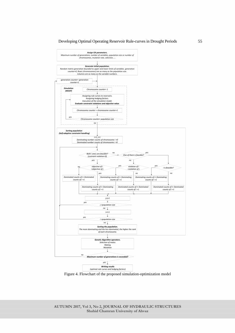
Developing Optimal Operating Reservoir Rule-curves in Drought Periods
AUTUMN 2017, Vol 3, No 2, JOURNAL OF HYDRAULIC STRUCTURES
Shahid Chamran University of Ahvaz
55
Generate initial population.Random matrix generation bounded to upper and lower limits of variables. generation
counter=0, Rows (chromosomes) are as many as the population size.Columns are as many as the variable numbers.
Chromosome counter= 1 Chromosome counter= 1
Assigning rule-curves to reservoirs.Assigning hedging factors.
Execution of the simulation model.Evaluate constraint violations and objective value.
Assigning rule-curves to reservoirs.Assigning hedging factors.
Execution of the simulation model.Evaluate constraint violations and objective value.
Chromosome counter = chromosome counter+1Chromosome counter = chromosome counter+1
Chromosome counter< population sizeChromosome counter< population size
no
yes
Both i and j are feasible?(costraint violation=0)
Both i and j are feasible?(costraint violation=0)
Genetic Algorithm operators.Selection of mates
MatingMutation
Genetic Algorithm operators.Selection of mates
MatingMutation
Sorting population (Self-adaptive constraint handling)
yes
no
Maximum number of generations is exceeded?Maximum number of generations is exceeded?
Writing results (optimal rule-curves and hedging factors)
Writing results (optimal rule-curves and hedging factors)
Dominating counts of i= Dominating counts of i +1
Dominating counts of i= Dominating counts of i +1
Simulation (WEAP)
objective of i <objective of j
objective of i <objective of j
violation of i<violation of j
violation of i<violation of j
Dominated counts of i= Dominated counts of i +1
Dominated counts of i= Dominated counts of i +1
yes
yes
i=1, j=1Dominating number counts of chromosome i =0Dominated number counts of chromosome i =0
i=1, j=1Dominating number counts of chromosome i =0Dominated number counts of chromosome i =0
j=j+1j=j+1
i=i+1i=i+1
i <population sizei <population size
j <population sizej <population size
Dominating counts of i= Dominating counts of i +1
Dominating counts of i= Dominating counts of i +1
Dominated counts of i= Dominated counts of i +1
Dominated counts of i= Dominated counts of i +1
no
no
no
yes
Sorting the population.The more dominating and the less dominated, the higher the rank
of each chromosome.
Sorting the population.The more dominating and the less dominated, the higher the rank
of each chromosome.
generation counter= generation counter+1
generation counter= generation counter+1
yes
yes
no
no
One of them is feasible? One of them is feasible? yes
no
i is feasible?i is feasible?
Dominating counts of i= Dominating counts of i +1
Dominating counts of i= Dominating counts of i +1
Dominated counts of i= Dominated counts of i +1
Dominated counts of i= Dominated counts of i +1
yes
no
Assign GA parameters.Maximum number of generations, number of variables, population size or number of
chromosomes, mutation rate, selection, ...
Figure 4. Flowchart of the proposed simulation-optimization model
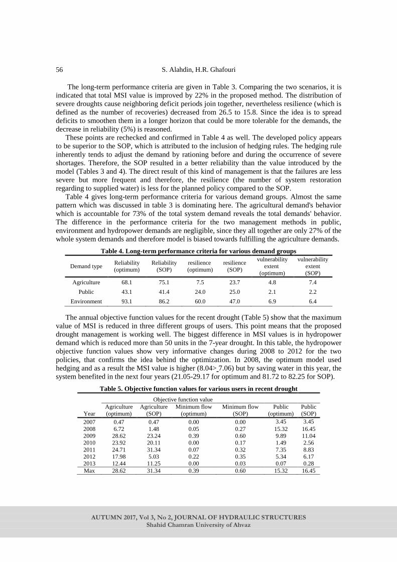
S. Alahdin, H.R. Ghafouri
AUTUMN 2017, Vol 3, No 2, JOURNAL OF HYDRAULIC STRUCTURES
Shahid Chamran University of Ahvaz
56
The long-term performance criteria are given in Table 3. Comparing the two scenarios, it is
indicated that total MSI value is improved by 22% in the proposed method. The distribution of
severe droughts cause neighboring deficit periods join together, nevertheless resilience (which is
defined as the number of recoveries) decreased from 26.5 to 15.8. Since the idea is to spread
deficits to smoothen them in a longer horizon that could be more tolerable for the demands, the
decrease in reliability (5%) is reasoned.
These points are rechecked and confirmed in Table 4 as well. The developed policy appears
to be superior to the SOP, which is attributed to the inclusion of hedging rules. The hedging rule
inherently tends to adjust the demand by rationing before and during the occurrence of severe
shortages. Therefore, the SOP resulted in a better reliability than the value introduced by the
model (Tables 3 and 4). The direct result of this kind of management is that the failures are less
severe but more frequent and therefore, the resilience (the number of system restoration
regarding to supplied water) is less for the planned policy compared to the SOP.
Table 4 gives long-term performance criteria for various demand groups. Almost the same
pattern which was discussed in table 3 is dominating here. The agricultural demand's behavior
which is accountable for 73% of the total system demand reveals the total demands' behavior.
The difference in the performance criteria for the two management methods in public,
environment and hydropower demands are negligible, since they all together are only 27% of the
whole system demands and therefore model is biased towards fulfilling the agriculture demands.
Table 4. Long-term performance criteria for various demand groups
Demand type Reliability
(optimum)
Reliability
(SOP)
resilience
(optimum)
resilience
(SOP)
vulnerability
extent
(optimum)
vulnerability
extent
(SOP)
Agriculture 68.1 75.1 7.5 23.7 4.8 7.4
Public 43.1 41.4 24.0 25.0 2.1 2.2
Environment 93.1 86.2 60.0 47.0 6.9 6.4
The annual objective function values for the recent drought (Table 5) show that the maximum
value of MSI is reduced in three different groups of users. This point means that the proposed
drought management is working well. The biggest difference in MSI values is in hydropower
demand which is reduced more than 50 units in the 7-year drought. In this table, the hydropower
objective function values show very informative changes during 2008 to 2012 for the two
policies, that confirms the idea behind the optimization. In 2008, the optimum model used
hedging and as a result the MSI value is higher (8.04> 7.06) but by saving water in this year, the
system benefited in the next four years (21.05-29.17 for optimum and 81.72 to 82.25 for SOP).
Table 5. Objective function values for various users in recent drought
Year
Objective function value
Agriculture
(optimum)
Agriculture
(SOP)
Minimum flow
(optimum)
Minimum flow
(SOP)
Public
(optimum)
Public
(SOP)
2007 0.47 0.47 0.00 0.00 3.45 3.45
2008 6.72 1.48 0.05 0.27 15.32 16.45
2009 28.62 23.24 0.39 0.60 9.89 11.04
2010 23.92 20.11 0.00 0.17 1.49 2.56
2011 24.71 31.34 0.07 0.32 7.35 8.83
2012 17.98 5.03 0.22 0.35 5.34 6.17
2013 12.44 11.25 0.00 0.03 0.07 0.28
Max 28.62 31.34 0.39 0.60 15.32 16.45
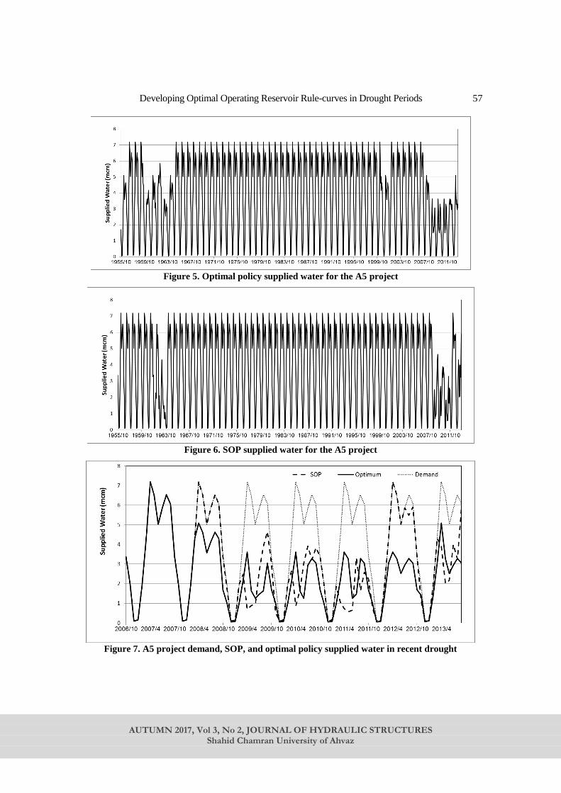
Developing Optimal Operating Reservoir Rule-curves in Drought Periods
AUTUMN 2017, Vol 3, No 2, JOURNAL OF HYDRAULIC STRUCTURES
Shahid Chamran University of Ahvaz
57
Figure 5. Optimal policy supplied water for the A5 project
Figure 6. SOP supplied water for the A5 project
Figure 7. A5 project demand, SOP, and optimal policy supplied water in recent drought

S. Alahdin, H.R. Ghafouri
AUTUMN 2017, Vol 3, No 2, JOURNAL OF HYDRAULIC STRUCTURES
Shahid Chamran University of Ahvaz
58
For A5 project which is located in Zohreh system downstream (see Figure 1), the details of
operation (water supplied) are presented by SOP and optimal rule-curves in Figures 5 and 6.
Visual comparison of two policies' performances (SOP and optimal rule-curve with hedging) are
illustrated in Figure 7. This figure graphically shows the superiority of the new routine through
the smooth behavior, good correlation with demand and less severe deficits.
Since this optimal operation policy is prescribed based on the whole 58-year historical
records, trigger water levels are general and synchronized for all hydrological conditions
experienced including successive droughts, particularly 9-year in the initial and 7-year recent
drought in the last stages of the record. But if in a particular event another policy performs better
(SOP in 1999-2000, Figures 5 and 6), it corresponds to the peculiar hydrologic attributes of that
event. However, it is known that in the SOP, if insufficient water is available to satisfy the
demands, the reservoir releases all the water available and becomes empty; if inflow is high, the
reservoir will fill and spill its excess water. Becuse this policy does not provide a mechanism for
decreasing release in the early stages or during indications of impending drought.
Optimal rule-curves coupling to hedging rules for Kheirabad, Kosar, and Chamshir reservoirs
are shown in Figs. 8–10. These monthly trigger levels of reservoir are optimized for
management during droughts.
Figure 8. Optimal rule-curves for Kheirabad
Figure 9. Optimal rule-curves for Kosar

Developing Optimal Operating Reservoir Rule-curves in Drought Periods
AUTUMN 2017, Vol 3, No 2, JOURNAL OF HYDRAULIC STRUCTURES
Shahid Chamran University of Ahvaz
59
Figure 10. Optimal rule-curves for Chamshir
The rule-curves structures illustrated in Figures 8-10 indicate that the implementation of
Formulas 5 and 6 in the developed model algorithm as constraints is logical. As a result, the
difference between two susequent coordinate points and the difference between the first and the
last month of water year is kept bounded based on the considerations and operational views of
the water resource managers.
5. Conclusion In this paper, a drought management simulation-optimization model was introduced to derive
the rule-curves and rationing factors for multi-purpose multi-reservoir systems. The system of
reservoirs and demands is mathematically simulated using a flexible and general WEAP model.
In the simulation model, all physical constraints of the case-study are systematically satisfied. In
a higher level, a self-adaptive GA is used to optimize the reservoirs rule-curves and hedging
factors with the objective function of modified shortage index (MSI). The model was applied to
a real three-reservoir drought-stricken system. After the optimization, the system performance
was compared to the results of the SOP. The rule-curves derived from the historical 58-year
period data systematically consider different climate conditions experienced by the system and
would be able to manage similar conditions in the future. The proposed operating rules can
mitigate the water shortage consequences by rationing current demands and saving water for
future uses in drought periods. In terms of agriculture, public and hydropower supply of
demands, with regard to the performance criteria, the model outperforms the SOP.
6. References 1. Tu M. Y., Hsu N. S., Yeh W. W. G., (2003). Optimization of reservoir management and
operation with hedging rules. Journal of Water Resources Planning and Management,
DOI: 10.1061/(ASCE)0733-9496(2003)129:2(86), 86–97.
2. Shih J. S., ReVelle C., (1994). Water-supply operations during drought: Continuous
hedging rule. Journal of Water Resources Planning and Management, DOI:
10.1061/(ASCE)0733-9496(1994)120:5(613), 613–629.
3. Srinivasan K., Philipose M. C., (1996). Evaluation and selection of hedging policies
using stochastic reservoir simulation. Water Resources Management, 10(3), 163–188.
4. Srinivasan K., Philipose M. C., (1998). Effect of hedging on over year reservoir
performance. Water Resources Management, 12(2), 95–120.

S. Alahdin, H.R. Ghafouri
AUTUMN 2017, Vol 3, No 2, JOURNAL OF HYDRAULIC STRUCTURES
Shahid Chamran University of Ahvaz
60
5. Draper A. J., Lund J. R., (2004). Optimal hedging and carryover storage value. Journal
of Water Resources Planning and Management, 130(1), 83– 87.
6. You J. Y., Cai X. M., (2008a). Hedging rule for reservoir operations. 1. A theoretical
analysis. Water Resources Research, 44(1), W01415.
7. You J. Y., Cai X. M., (2008b). Hedging rule for reservoir operations. 2. A numerical
model. Water Resources Research, 44(1), W01416.
8. Shiau J. T. (2009). Optimization of reservoir hedging rules using multi-objective genetic
algorithm. Journal of Water Resources Planning and Management, DOI:
10.1061/(ASCE)0733-9496(2009)135:5(355), 355–363.
9. Shiau J. T., (2011). Analytical optimal hedging with explicit incorporation of reservoir
release and carryover storage targets. Water Resources Research, VOL. 47, W01515,
DOI: 10.1029/2010WR009166.
10. Eum H., Kim Y., Palmer R.N., (2011). Optimal drought management using sampling
stochastic dynamic programming with a hedging rule. Journal of Water Resources
Planning and Management 137(1):113–122. DOI: 10.1061/(ASCE)WR.1943-
5452.0000095.
11. Dariane A., B., Karami F., (2014). Deriving Hedging Rules of Multi-Reservoir System
by Online Evolving Neural Networks. Water Resources Management. DOI:
10.1007/s11269-014-0693-0.
12. Ahmadianfar I., Adib A., Taghian M., (2016). Optimization of Fuzzified Hedging Rules
for Multipurpose and Multi-reservoir Systems. DOI: 10.1061/(ASCE)HE.1943-
5584.0001329.
13. Huang C., Zhao J., Wang Z., Shang W., (2016). Optimal Hedging Rules for Two-
Objective Reservoir Operation: Balancing Water Supply and Environmental Flow.
Journal of Water Resources Planning and Management, 04016053, DOI:
10.1061/(ASCE)WR.1943-5452.0000699.
14. Shih J. S., ReVelle C., (1995). Water supply operations during drought: A discrete
hedging rule. European Journal of Operational Research, 82(1), 163–175.
15. Tu M. Y., Hsu N. S., Tsai F. T. C., Yeh W. W. G., (2008). Optimization of hedging
rules for reservoir operations. Journal of Water Resources Planning and Management,
DOI: 10.1061/(ASCE)0733-496(2008)134:1(3), 3–13.
16. Guo X., Hu T., Zeng X., Li X., (2013). Extension of parametric rule with the hedging
rule for managing multi-reservoir system during droughts. Journal of Water Resources
Planning Management, 10.1061/(ASCE) WR.1943-5452.0000241, 139–148.
17. Taghian M., Rosbjerg D, Haghighi A., Madsen H., (2013). Optimization of
Conventional Rule-curves Coupled with Hedging Rules for Reservoir Operation. Journal
of Water Resources Planning and Management, DOI: 10.1061/(ASCE)WR.1943-
5452.0000355.
18. Ashrafi S.M., Ashrafi S.F., Moazami S., (2017). Developing Self-adaptive Melody
Search Algorithm for Optimal Operation of Multi-reservoir Systems. Journal of
Hydraulic Structures, 3(1):35-48, DOI: 10.22055/jhs.2017.13282.
19. Zhao J., Cai X., Wang Z., (2011). Optimality conditions for a two-stage reservoir
operation problem. Water Resources Research, 47, W08503, DOI:
10.1029/2010WR009971.
20. Hydrologic Engineering Center, Reservoir yield; generalized computer program, 23-J2-
L245. U.S. Army Corps of Engineers, Davis, Calif, 1966.

Developing Optimal Operating Reservoir Rule-curves in Drought Periods
AUTUMN 2017, Vol 3, No 2, JOURNAL OF HYDRAULIC STRUCTURES
Shahid Chamran University of Ahvaz
61
21. Hydrologic Engineering Center, Hydrologic engineering methods for water resources
development; Vol. 8, reservoir yield, U.S. Army Corps of Engineers, Davis, Calif, 1975.
22. Hsu S. K., (1995). Shortage indices for water-resources planning in Taiwan. Journal of
Water Resources Planning and Management, 121(2), 119–131.
23. Ahmadi Najl A., Haghighi A., Samani H.M.V., (2016). Deriving Optimum Trade-Off
between the Benefits and Costs of Inter-basin Water Transfer Projects. International
Journal of Optimization in Civil Engineering, 6(2):173-185.
24. Suen J. P., Wayland E. J., (2006). Reservoir management to balance ecosystem and
human needs; Incorporating the paradigm of the ecological flow regime. Water
Resources Research, VOL. 42, W03417, DOI: 10.1029/2005WR004314.
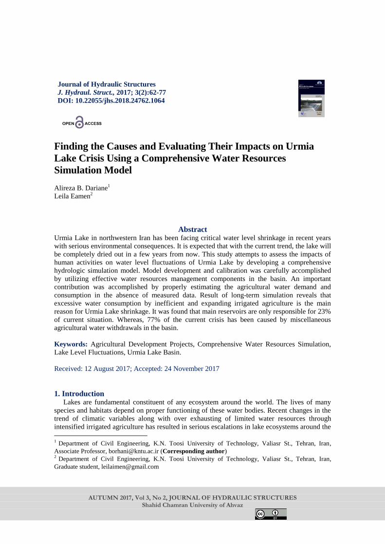
AUTUMN 2017, Vol 3, No 2, JOURNAL OF HYDRAULIC STRUCTURES
Shahid Chamran University of Ahvaz
Journal of Hydraulic Structures
J. Hydraul. Struct., 2017; 3(2):62-77
DOI: 10.22055/jhs.2018.24762.1064
Finding the Causes and Evaluating Their Impacts on Urmia
Lake Crisis Using a Comprehensive Water Resources
Simulation Model
Alireza B. Dariane1
Leila Eamen2
Abstract Urmia Lake in northwestern Iran has been facing critical water level shrinkage in recent years
with serious environmental consequences. It is expected that with the current trend, the lake will
be completely dried out in a few years from now. This study attempts to assess the impacts of
human activities on water level fluctuations of Urmia Lake by developing a comprehensive
hydrologic simulation model. Model development and calibration was carefully accomplished
by utilizing effective water resources management components in the basin. An important
contribution was accomplished by properly estimating the agricultural water demand and
consumption in the absence of measured data. Result of long-term simulation reveals that
excessive water consumption by inefficient and expanding irrigated agriculture is the main
reason for Urmia Lake shrinkage. It was found that main reservoirs are only responsible for 23%
of current situation. Whereas, 77% of the current crisis has been caused by miscellaneous
agricultural water withdrawals in the basin.
Keywords: Agricultural Development Projects, Comprehensive Water Resources Simulation,
Lake Level Fluctuations, Urmia Lake Basin.
Received: 12 August 2017; Accepted: 24 November 2017
1. Introduction Lakes are fundamental constituent of any ecosystem around the world. The lives of many
species and habitats depend on proper functioning of these water bodies. Recent changes in the
trend of climatic variables along with over exhausting of limited water resources through
intensified irrigated agriculture has resulted in serious escalations in lake ecosystems around the
1 Department of Civil Engineering, K.N. Toosi University of Technology, Valiasr St., Tehran, Iran,
Associate Professor, [email protected] (Corresponding author) 2 Department of Civil Engineering, K.N. Toosi University of Technology, Valiasr St., Tehran, Iran,
Graduate student, [email protected]

Finding the Causes and Evaluating Their Impacts on Urmia Lake Crisis …
AUTUMN 2017, Vol 3, No 2, JOURNAL OF HYDRAULIC STRUCTURES
Shahid Chamran University of Ahvaz
63
globe. Nevertheless, in some cases like the Aral Sea the consequence has been devastating
leaving a permanent damage without any hope of reconstructing the original system. Obviously,
the first step in solving any problem is to get a proper and sufficient knowledge of the problem
itself.
On the other hand, natural systems are very complicated and usually require extensive time,
expertise, and nationwide willingness to tackle the problem. This requires having a multi-
objective prospective of the problem so that a tradeoff could be made between the expansions of,
for example, water utilization projects and the wellbeing of the basin ecosystem. This is another
way of setting a balance between the short term benefits from water utilization projects and the
long term damages caused by altering the ecosystem of the basin. Through this process the
optimum level of developments could be established. Moreover, the consequences of
overexploitation of water resources of the basin on key components of the system can be
determined through these investigations. Therefore, a comprehensive study should consist of
modeling all factors that are important in shaping the future of the basin.
Human activities have a substantial impact on the quantity and quality of water resources of a
basin, mainly through extended irrigated agricultural practices. An ongoing population growth,
water pollution and lack of efficient water supply system along with competitions among
different water use sectors for maximizing their share of water consumption are main factors,
besides the climate change, that threaten the sustainability of water resources systems around the
world. As a result, the number of basins with water scarcity crisis and irreparable damages, like
the Aral Sea basin, is continuously increasing. Under these circumstances, proper management
and planning of water resources for allocating the scarce available water becomes very crucial.
On the other hand, basin planning that considers only one aspect of water use, such as the
agriculture, would eventually intensify the problem by neglecting the role of other sectors of the
system. Hence, the right solution would be through adopting an integrated water resources
management (IWRM) approach for the basin. Successful IWRM requires strong political
supports and is essential for sustainable use of water resources through environmental
considerations. One of the first steps in integrated water resources management is to evaluate the
amount of water resources and the demands of the basin and go through a long term simulation
to find out how the system behaves. This is accomplished by developing comprehensive
simulation models.
There are several basin wide simulation models that have been used in IWRM studies. Sulis
and Sechi (2013) made a comparison of five generic basin-wide simulating models including
AQUATOOL (Valencia Polytechnic University), MODSIM (Colorado State University),
RIBASIM (DELTARES), WARGI-SIM (University of Cagliari) and WEAP (Stockholm
Environmental Institute) [1]. There is wide range of researchers find the Water Evaluating and
Planning system (WEAP) a powerful tool to simulate water resources and demands of river
basins and investigate results of different development, water policy and other scenarios on
water balance of the basin including Raskin et al. (1992), Levite et al. (2003), Bharati et al.
(2009) and Mourad and Alshihabi (2016) [2,3,4,5]. Hashemi et al. (2010) proposed an integrated
methodological framework to implement IWRM in Urmia Lake basin [6].
Urmia Lake is a terminal lake without any outflow. Thus, evaporation is the only means for
the water loss through the Lake. Therefore, considering the large water surface area of the Lake,
any change in the evaporation rate would directly influence the Lake Water Level (LWL). The
only other means by which the LWL changes, is through the Lake inflow. Any change in
precipitation and temperature not only affects the evaporation rate from the Lake surface, but
also changes the demands for water throughout the basin and hence the inflows to the Lake. The

A. B. Dariane, L. Eamen
AUTUMN 2017, Vol 3, No 2, JOURNAL OF HYDRAULIC STRUCTURES
Shahid Chamran University of Ahvaz
64
continuous development of irrigated agricultural projects throughout the basin in the past
decades along with changes in the trend of precipitation and temperature have worked together
to dry up nearly 90% of the Lake surface today [7]. It is also interesting to note that the long
term mean LWL of the Lake Urmia, which was about 1276 metre (m) during 1976-1998 period,
dropped as much as 4.9 m during 1999-2009 decade [8].
Other studies also point out that the climate change and irrigated agriculture are the main
factors affecting Urmia Lake water level [e.g. 9,10,11]. A main problem with the past studies in
this basin is the lack of water demand and consumption, mainly agricultural, that made them to
use rough estimations. It is evident that without any reliable measured data, rough assumptions
could lead us to erroneous results. Therefore, this paper attempts to solve this problem through
developing a comprehensive basin-wide simulation model, which once calibrated could be used
for the evaluation of different planning scenarios. Also, it would be used to evaluate the impacts
of agricultural water use on the LWL by implementing different scenarios. Through this the role
of each water use sector (especially agriculture) in causing the current critical situation of the
Lake is determined. This information could be used for finding solutions to revive the Lake and
also for laying out the future plan of the basin.
1.1. Study Area Urmia Lake basin with an area of about 52 thousand square kilometres is located in
northwestern Iran. Three provinces sharing the basin are west Azerbaijan, east Azerbaijan and
Kurdistan. Main rivers discharging into the Lake are Zarrineroud, Simineroud, Ajichay,
Shahrchay, Sufichay, Mahabadroud, Godarroud, Ghalechay, Barandouzchay, Nazloochay,
Rozechay and Zoolachay. During recent decades various development projects were proposed in
the basin. Some of these projects are now in operation while some others are under construction
or feasibility study phases. In this study six main operational reservoirs are considered in the
simulation model, including Boukan, Mahabad, Shahrchay, Alavian, Hassanlou and Nahand
reservoirs. Figure (1) shows the location of Urmia Lake basin, main rivers and main operational
reservoirs.
Fig. 1 The location of Urmia Lake basin, main rivers and six operational reservoirs
Average annual mean temperature and precipitation of the basin shows the climatic condition

Finding the Causes and Evaluating Their Impacts on Urmia Lake Crisis …
AUTUMN 2017, Vol 3, No 2, JOURNAL OF HYDRAULIC STRUCTURES
Shahid Chamran University of Ahvaz
65
during 1966-2012 period (Figure 2). As it can be seen from Figure 2, during critical decade of
1995-2004, precipitation mostly remained below the long-term average (360 mm), while at the
same time above average temperatures (11°C) were observed, indicating a critical condition on
water resources of the basin. High temperatures result in increased agricultural water demand,
whereas low precipitations limit the amount of water production in the basin. Together, they can
cause severe drought and stressful condition as it was also observed during those years in the
region. Year 1995 is also the period where the shrinkage in the Lake Urmia began (see Figure 5)
and the lake level continued to fall up to now. It is also interesting to note that although after
2004 the precipitation began to rise above the long-term average (Figure 2), the lake level
decline did not stop and continued to fall to more sever lower levels (Figure 5), probably due to
persistent more higher than normal temperatures resulting in higher water demands throughout
the basin.
Fig. 2 Mean annual temperature and precipitation of the basin
Figure (3) shows total inflow to the Lake during the study period. As it can be seen from this
Figure, during critical period of 1995-2012 the inflow to the Lake is mostly below the long-term
average (solid line). We can divide the critical period beginning from 1995 into two distinct
period of 1995-2004 and 2004-2012. During the first decade-long critical period, precipitation is
considerably below average, temperature is slightly above average (Figure 2), and annual lake
inflow has sharply dropped below average (i.e., 2904 million cubic metre (mcm)) with an
exception in 2002 (Figure 3), probably as a result of consistent precipitation rise which began in
1998 and relatively near normal annual temperature during this year. During the second critical
period, temperature is even higher and well above the long-term average, but precipitation has
also increased to above normal levels (Figure 2). However, total inflow has continued to stay in
below average condition (Figure 3) regardless of higher precipitations, which could be attributed
to exceptionally higher temperatures during these years. Regardless of the aforementioned trends
and variations in the precipitation trend, the lake level has continued to drop sharply since 1995
throughout the last year in the study period (i.e., 2012).
150
200
250
300
350
400
450
500
550
600
650
7
8
9
10
11
12
13
14
15
19
66
19
68
19
70
19
72
19
74
19
76
19
78
19
80
19
82
19
84
19
86
19
88
19
90
19
92
19
94
19
96
19
98
20
00
20
02
20
04
20
06
20
08
20
10
20
12
Rai
nfa
ll (m
m)
Tem
pe
ratu
re ( C
)
Year
Temperature Temperature Average
Rainfall Rainfall Average

A. B. Dariane, L. Eamen
AUTUMN 2017, Vol 3, No 2, JOURNAL OF HYDRAULIC STRUCTURES
Shahid Chamran University of Ahvaz
66
Fig. 3 Total inflow to the Lake and its long term average (solid line)
2. Methods
2.1. Simulating Model Integrated approach in studying water resources systems requires the development of a proper
model which is capable of handling different components of the system with the needed
precision. In this study, WEAP software was used for developing a model to simulate the
interactions among water resources and demands on the one hand and the Urmia Lake level
fluctuations on the other. WEAP, developed at the Stockholm Environment Institute, is a policy
oriented simulating model which can be used for comprehensive water resources studies. It has
an integrated approach in simulating water resources systems [12]. The model, using a linear
programming algorithm, is capable of allocating available water among different demand sites
with user-defined priorities. In fact, the priorities could be set for both sources (i.e., reservoirs,
surface and groundwater) and sinks (i.e., water demand sites).
In this research, observed data during the historical period of 1966-2012 were used for the
development and evaluation of Urmia Lake basin model. Spatial information such as the basin
boundary, rivers and location of operational reservoirs were first generated in a Geographic
Information System (GIS) and then used in the WEAP model. Schematic of WEAP model for
Urmia Lake basin is shown in Figure (4).
Initial data required for modeling consists of surface and groundwater data, amounts of
agricultural, municipal and industrial water demands, and information on operational reservoirs
in the basin. The amount of agricultural water consumption, as the main water user in the basin,
was initially assumed and then estimated through calibration process for each sub-basin. The
initial assumption was made using the data obtained from the most recent Iranian agricultural
census [13], which is highly imprecise and does not represent the whole irrigated agriculture in
the basin. Moreover, the census data is available only for few specific years. Therefore, due to
uncertainties, monthly agricultural water demand for the whole historical period was estimated
during calibration process using a nonlinear development trend as explained in the following
section.

Finding the Causes and Evaluating Their Impacts on Urmia Lake Crisis …
AUTUMN 2017, Vol 3, No 2, JOURNAL OF HYDRAULIC STRUCTURES
Shahid Chamran University of Ahvaz
67
Fig. 4 Schematic of Urmia Lake basin water resources system model in WEAP
It should be mentioned that in most developing countries, like Iran, surveys and censuses are
not processed regularly each year but rather they are gathered every few years. Therefore, valid
information about the amounts and characteristics of water resources and demands, mostly for
agricultural use, are unavailable in a regular basis and estimating methods should be applied to
fill the gaps. Meanwhile, the surveys are very rough and mainly concentrate on large areas.
Noting that the size of agricultural fields in Iran is mainly small and unlike many countries
farmers own scattered small size fields, an accurate estimation of irrigated area is very
challenging.
2.2. Calibration Method Model calibration in a basin with many uncertainties that mainly arise from poor data, both
quantitatively and qualitatively, is a tedious task and becomes even more complicated by
realizing that there is not even a single reliable comprehensive set of data measurement during
the whole period. Agricultural water consumption data throughout the Urmia Lake basin is only
measured in certain limited locations with an amount which is only a fraction of the total
irrigation water use throughout the basin. In fact, there are many unregistered wells, diversion
canals, and even Qanats with unknown water yield in the basin which are not counted in
censuses data gathering. Therefore, it is not possible to determine a certain figure that accounts
for the amount of water demand and/or consumption in the area per each time period. Based on
our knowledge from the region, we used a nonlinear trend for the agricultural water consumption
during the study period (1966-2012) to overcome the problem. The trend was linearized by
realizing four distinct periods in the historical data (Figure 5) as explained in the following:

A. B. Dariane, L. Eamen
AUTUMN 2017, Vol 3, No 2, JOURNAL OF HYDRAULIC STRUCTURES
Shahid Chamran University of Ahvaz
68
Period 1: 1966-1976 (mean LW L: 1275.81 m)
Period 2: 1977-1990 (mean LWL: 1275.80 m)
Period 3: 1991-1997 (mean LWL: 1277.12 m)
Period 4: 1998-2012 (mean LWL: 1273.14 m)
Fig. 5 Linearized agricultural demand coefficients during four periods
The first period indicates the initial stage with the least development in the basin until 1977
when the Boukan (see Figure 1) as the first major reservoir began to operate. Period 2 includes
the beginning of Boukan reservoir operation until 1991 when the Lake water level started to rise
(Figure 5) due to increased precipitation (Figure 2) and increased lake inflow (Figure 3). 1977 to
1991 was also the period of imposed Iraq war on Iran where the trend of various project
developments including the agriculture was very slow due to the nations’ budgetary limitations.
The third period is the era of so called “reconstruction” after the war. It also represents a
duration of high water level in the Urmia Lake due to above normal precipitations (Figure 2),
below normal temperatures (Figure 2), and mostly above normal inflows (Figure 3). In 1998 the
Lake began to fall below its mean LWL of 1276.1 m by that time, a trend which has consistently
continued up to now. Thus, the fourth period resembles the period of Lake Urmia shrinkage and
desiccation. The calibration process determines both the level of initial agricultural water
consumption in year 1966 and the slopes of developments during the above mentioned four
periods as shown in Figure 5 through a trial and error process.
Other parameters used in calibrating the model include evaporation rate from the Lake
surface, groundwater recharge after continued drought periods, and adjustments on agricultural
water supply by the main reservoirs. As it was explained earlier, there are uncertainties on some
measurements because they are not available either for the period or at the location of interest.
Lake evaporation rate from freshwater can be estimated using either evaporation pan
measurements or through certain relationships. However, for saltwater it is not possible to
directly use these procedures. And although we were able to establish a relationship between
evaporation rate from fresh and salt water using limited available data, it would be only a rough
estimate since the density of salt is also a factor in determining the actual evaporation from
saltwater surface. On the other hand, since the area of Urmia Lake is considerable (between 4000
to 6000 km2) a small change in the evaporation rate would have a substantial impact on the

Finding the Causes and Evaluating Their Impacts on Urmia Lake Crisis …
AUTUMN 2017, Vol 3, No 2, JOURNAL OF HYDRAULIC STRUCTURES
Shahid Chamran University of Ahvaz
69
volume of the water losses through evaporation. Therefore, the mass balance equation of the
Lake is highly sensitive to the rate of evaporation, and in the absence of precise measurements
and concerning the uncertainties inherent in the process, must be determined through calibration
using the initially estimated values.
Groundwater recharge is another important parameter in the basin water balance model which
must be also determined through calibration process in the absence of any data. The effect of
recharging groundwater through precipitation and surface water was included through applying
reductions on the river flow as a function of continued droughts. Therefore, the amount of
surface water used for recharging groundwater is assumed to be a function of both drought
intensity and its persistence. A coefficient was defined and found by calibration to adjust the
amount of total water used for recharging the groundwater in each sub-basin under a defined
drought condition. Therefore, three main categories are used for accomplishing the model
calibration where each may involve several decision variables. These include adjustments on
agricultural water demand during each of the above mentioned periods, adjustments on
evaporation from lake’s surface (saltwater), and finally adjustments on groundwater recharge
rate as function of continued drought period.
The objective of the calibration process is to minimize the sum of errors between the
observed and simulated LWLs during the historical period (1966-2012). A trial and error method
is used for calibrating the model. Statistical criteria used for evaluating the performance of the
model during the calibration and test periods are coefficient of determination (Equation 1),
Nash-Sutcliffe efficiency (Equation 2) and Root Mean Square Error (Equation 3).
𝑅2 = (∑ ((𝑂𝐿𝑖−𝑂𝐿̅̅ ̅̅ )(𝑆𝐿𝑖−𝑆𝐿̅̅̅̅ ))𝑛𝑖=1
√∑ (𝑂𝐿𝑖−𝑂𝐿̅̅ ̅̅ )2∑ (𝑆𝐿𝑖−𝑆𝐿̅̅̅̅ )
2𝑛𝑖=1
𝑛𝑖=1
)
2
(1)
𝑁𝑆𝐸 = 1 −∑ (𝑂𝐿𝑖−𝑆𝐿𝑖)
2𝑛𝑖=1
∑ (𝑂𝐿𝑖−𝑂𝐿̅̅ ̅̅ )2𝑛
𝑖=1
(2)
𝑅𝑀𝑆𝐸 = √∑ (𝑆𝐿𝑖−𝑂𝐿𝑖)
2𝑛𝑖=1
𝑛 (3)
Where, OLi and SLi are the observed and simulated LWLs at the beginning of month i, and
𝑂𝐿̅̅̅̅ and 𝑆𝐿̅̅ ̅ are the average of observed and simulated LWL data, respectively. Figure 6 shows
the flowchart of the model and its calibration process.

A. B. Dariane, L. Eamen
AUTUMN 2017, Vol 3, No 2, JOURNAL OF HYDRAULIC STRUCTURES
Shahid Chamran University of Ahvaz
70
Fig. 6 Flowchart showing the simulation model structure and its calibration
Figure (7) shows the calibrated and observed LWL of Urmia Lake during the study period
(1966-2012). A visual comparison of modeled and observed LWL indicates a good fit.
Moreover, the performance of the calibrated model was evaluated by coefficient of
determination (R2), Nash-Sutcliffe Index (NSE) and root mean square error (RMSE), where their
corresponding values were found as 0.98, 0.97 and 0.005 respectively.
Fig. 7 Simulated and observed LWL of Urmia Lake (1966-2012)
Scatter plot of monthly observed and simulated water level of the Lake for the study period is
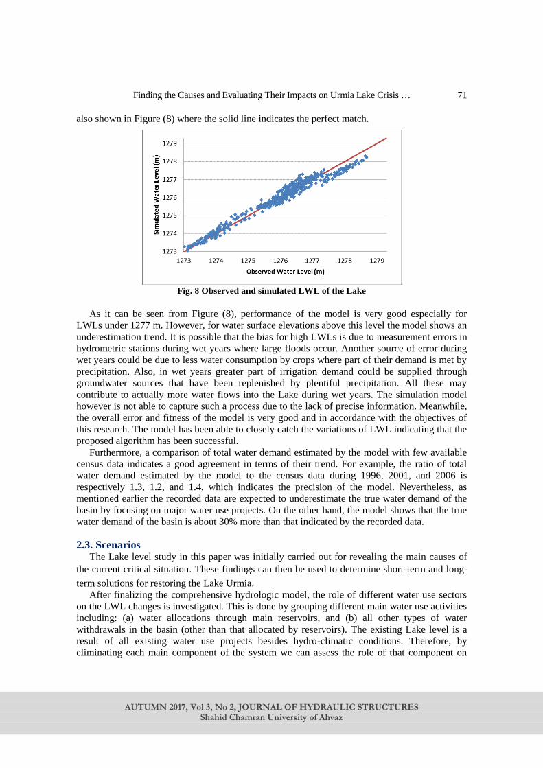
Finding the Causes and Evaluating Their Impacts on Urmia Lake Crisis …
AUTUMN 2017, Vol 3, No 2, JOURNAL OF HYDRAULIC STRUCTURES
Shahid Chamran University of Ahvaz
71
also shown in Figure (8) where the solid line indicates the perfect match.
Fig. 8 Observed and simulated LWL of the Lake
As it can be seen from Figure (8), performance of the model is very good especially for
LWLs under 1277 m. However, for water surface elevations above this level the model shows an
underestimation trend. It is possible that the bias for high LWLs is due to measurement errors in
hydrometric stations during wet years where large floods occur. Another source of error during
wet years could be due to less water consumption by crops where part of their demand is met by
precipitation. Also, in wet years greater part of irrigation demand could be supplied through
groundwater sources that have been replenished by plentiful precipitation. All these may
contribute to actually more water flows into the Lake during wet years. The simulation model
however is not able to capture such a process due to the lack of precise information. Meanwhile,
the overall error and fitness of the model is very good and in accordance with the objectives of
this research. The model has been able to closely catch the variations of LWL indicating that the
proposed algorithm has been successful.
Furthermore, a comparison of total water demand estimated by the model with few available
census data indicates a good agreement in terms of their trend. For example, the ratio of total
water demand estimated by the model to the census data during 1996, 2001, and 2006 is
respectively 1.3, 1.2, and 1.4, which indicates the precision of the model. Nevertheless, as
mentioned earlier the recorded data are expected to underestimate the true water demand of the
basin by focusing on major water use projects. On the other hand, the model shows that the true
water demand of the basin is about 30% more than that indicated by the recorded data.
2.3. Scenarios The Lake level study in this paper was initially carried out for revealing the main causes of
the current critical situation. These findings can then be used to determine short-term and long-
term solutions for restoring the Lake Urmia.
After finalizing the comprehensive hydrologic model, the role of different water use sectors
on the LWL changes is investigated. This is done by grouping different main water use activities
including: (a) water allocations through main reservoirs, and (b) all other types of water
withdrawals in the basin (other than that allocated by reservoirs). The existing Lake level is a
result of all existing water use projects besides hydro-climatic conditions. Therefore, by
eliminating each main component of the system we can assess the role of that component on

A. B. Dariane, L. Eamen
AUTUMN 2017, Vol 3, No 2, JOURNAL OF HYDRAULIC STRUCTURES
Shahid Chamran University of Ahvaz
72
LWL changes through long term model simulation.
Water use scenarios are defined as follows:
1. No Operational Reservoirs (NoRes): Impact of operational reservoirs and their water
demands (mainly agricultural) is evaluated in this scenario by eliminating them from the
system according to their starting operation date.
2. No Other Withdrawals (NoWdr): All other water withdrawals (mainly agricultural)
are eliminated to assess their role on Lake level fluctuations.
3. No Reservoirs and No Other Withdrawals (NoRes & Wdr): This scenario is
implemented to show the impact of combined actions. In fact, it shows a situation where
human related water use activities in the basin are removed and thus indicates the natural
and intact basin condition.
It is worthwhile to mention that in Urmia basin nearly 92% of water consumption is used by
agriculture, 6% by municipal, and the remaining 2% by industrial sectors. Therefore, agriculture
is the main water use sector in the area either through regulated reservoir releases or other types
of water withdrawals from surface and groundwater sources.
According to a study the minimum acceptable water level required for the Lake to survive
ecologically is found to be 1274 m [14]. The Lake is home to a unique brine shrimp species,
artemia urmiana, and supports many species of reptiles, amphibians and mammals [15]. Water
levels less than this elevation may cause serious hazards on ecology of the Lake including the
artemia population and the basin as well.
3. Results and Discussions The normal values are usually calculated using the whole study period, i.e., 1966-2012 in this
case. However, noting that the lake has entered a completely drying and abnormal situation more
than a decade ago, such a calculation would not represent the lake hydrology and the conclusions
derived from these figures could be erroneous. For example, long-term mean LWL would be
1275 meters using 1966-2012 period which indicates that years 1968 through 2000 (about
consecutive 32 years) are all above normal or otherwise wet periods. The mean LWL, surface
area and storage volume calculated using the whole period is 1275.15 m, 5076 km2, and 30335
mcm, respectively. This divides the lake into two distinct period of above normal 1966-2000 and
below normal 2001-2012. However, if only the healthy period of the lake is considered, using
the years 1966 through 2000 mean LWL, surface area and storage would be 1276.03 m, 5405
km2, and 34944 mcm, respectively. In this case, alternating above and below normal situations
are observed. Obviously in both cases the period after year 2000 is considered as abnormally
dry.
The calibrated model was used to evaluate the impacts of different human activities on water
level fluctuations of the Lake. As explained in the previous section, the role of different activities
including reservoir constructions and other miscellaneous water withdrawals on current Lake
crisis is investigated.
Water levels of Urmia Lake under different water resources development scenarios are found
by removing the corresponding activity and then simulating the system using the calibrated
WEAP model. As it can be seen from Figure (9), the impact of NoWdr scenario is considerably
greater than that of NoRes on Urmia Lake water level fluctuations. This is in contradiction to
what many environmental activists in Iran had been calling for, at least during the last decade
where the reservoir construction was blamed as the main source of Lake water shrinkage.

Finding the Causes and Evaluating Their Impacts on Urmia Lake Crisis …
AUTUMN 2017, Vol 3, No 2, JOURNAL OF HYDRAULIC STRUCTURES
Shahid Chamran University of Ahvaz
73
However, our investigation shows (not included in this paper) that also unlike what official
authorities have been claiming the climate change is not to be blamed for the extent of current
situation. The current situation is rather a direct consequence of ignoring the principles of
sustainable development in the region. At least in the last three decades the development of
agriculture industry with a goal of self-sufficiency has been the main objective in the country.
Therefore, it is not surprising to see the rapidly growing demand for water and the rushing
emergence of various water resources projects in the basin during the “reconstruction” era after
the early 1990s when Iran-Iraq war ended. A closer look at the slope of agricultural water
demand after 1992 (periods 3 and 4) in Figure 5 makes it clear that water consumption gained a
rapid slope after this date.
According to our results, by removing water consumption through “Other Withdrawals” (i.e.,
NoWdr scenario) the LWL would have risen by 5.2 meters (equivalent to 22,325 mcm in
volumetric measures) in 2012. Whereas, for removing water consumptions through operational
reservoirs (i.e., NoRes scenario) the rise in LWL would be only 1.9 meters (6,676 mcm of lake
water), which indicates much less impact than the aforementioned scenario. As it can be seen
from Figure (9), combined removal of “No Other Withdrawals” and “No Operational
Reservoirs” scenarios would increase the LWL by about 6.4 meters (29001 mcm of water) in
year 2012. Therefore, main reservoirs are only responsible for 23% of current situation.
Whereas, miscellaneous agricultural water withdrawals are responsible for 77% of the current
Lake Urmia crisis.
Fig. 9 Comparison of LWL under different water resources development scenarios
Observed and simulated LWL under different scenarios at the ending year of the four time
stages are shown in Figure 10. As it can be seen from this Figure, in all four years the water
withdrawal by means other than the operational reservoirs (i.e., NoWdr scenario) has the most
considerable impact on LWL. In addition, the impact of operational reservoirs (NoRes) becomes
more considerable as we proceed through the time as a consequence of new reservoir
construction. For example, removing reservoirs during periods 1 and 2 has insignificant impact
on LWL which is evident by comparing the observed and NoRes LWLs. However, the gap
becomes wider as we move to periods 3 and 4. It should be mentioned that in the first time stage
(1966-1976) no reservoir was yet built in the basin. Therefore, as it can be seen from Figure 10
the LWL for NoRes option is the same as the observed level. Moreover, the impact of water use

A. B. Dariane, L. Eamen
AUTUMN 2017, Vol 3, No 2, JOURNAL OF HYDRAULIC STRUCTURES
Shahid Chamran University of Ahvaz
74
by “other withdrawals” also increases with time as a result of increased water demand. While
removing other withdrawals (i.e., NoWdr) in the first stage raises the LWL by less than 3 meters,
in the second (1977-1990), third (1991-1997) and final stage (1998-2012) it raises the LWL by
about 3.6, 3.5, and 5.2 meters, respectively. A review of the gap between the observed LWL and
NoWdr scenario reveals the growing extent of miscellaneous water use projects in the basin
during these years.
Fig. 10 Comparison of LWL under water resources development scenarios at the ending year of
four time periods
Since Urmia is a shallow lake, small changes on the Lake level considerably affects its
surface area. Figure 11 compares the surface area of Urmia Lake under different water resources
development scenarios during the four periods. The observed surface area of the Lake was about
3.4 thousand square kilometers in 2012, while it would have reached to about 6 thousand square
kilometers if both operational reservoirs and all other withdrawals were removed from the
system. It is noteworthy to mention that in the same year only by eliminating other withdrawals
the Lake surface area would have reached to 5.4 thousand square kilometers, an increase of
about 1.9 thousand square kilometers. Thus, we would have seen a normal situation in Urmia
Lake even by having all the existing operational reservoirs but removing all other withdrawals.
On the other hand, under the situation of NoRes, as it is shown in Figure 11, the area of the Lake
would have increased only by 0.7 thousand square kilometers in 2012.
Finding the Causes and Evaluating Their Impacts on Urmia Lake Crisis …
AUTUMN 2017, Vol 3, No 2, JOURNAL OF HYDRAULIC STRUCTURES
Shahid Chamran University of Ahvaz
75
Fig. 11 Comparison of Urmia Lake surface area under different scenarios at the ending year of four
time periods
The results of this study reveal that the number one factor in causing the current Urmia Lake
crisis is the miscellaneous water withdrawals throughout the basin by means other than
reservoirs. These water withdrawals consist of legal and illegal surface and in specific
groundwater. In the surface water, there are also small reservoirs mostly without any
documentations and records that were constructed by local authorities mainly during the last
three decades. Since these reservoirs are very small and numerous, and mostly without any
documentation, we do not include them in “operational reservoirs” category which consists only
of large reservoirs in the basin. There are also many illegally constructed wells which are
scattered around the basin and in specific near the Lake shores. Nevertheless, the total water
utilized through these small projects has much considerable impact on the LWL than the main
reservoirs. These projects were made gradually through the time by local people without any
concern on their long-term impact. People in the region highly rely on these projects which are
twisted with their daily life. Therefore, there seems to be no short-term and quick solution to the
problem. However, noting that the current irrigation efficiency in the area is less than 35% and
that 92% of the total water utilization is by the agriculture, a long-term solution should aim at
modernizing the irrigation system and freeing more water into the Lake.
Unfortunately, the fact is that the current critical situation of the Urmia Lake is a direct
consequence of neglecting the Lake itself in various water resources projects and agricultural
developments in the basin during last half a century. In developing countries where private
sector has the least role in regional and national decision makings, local and national water and
agricultural authorities are mainly responsible for the crises created. Nevertheless, this study
shows that unless a comprehensive and integrated approach is followed and implemented, the
current critical condition of Urmia Lake will be even more escalated in the future considering the
climate change. The projected LWL reveals that the existence of this water body which is very
crucial for the whole northwestern Iran needs prompt and quick attention. The solution should
consist of short-term and long-term comprehensive action plans and should consider all effective
components in the region.

A. B. Dariane, L. Eamen
AUTUMN 2017, Vol 3, No 2, JOURNAL OF HYDRAULIC STRUCTURES
Shahid Chamran University of Ahvaz
76
4. Conclusion A simulation model was developed using WEAP software to study the water resources
system of Urmia Lake basin. A calibration procedure was proposed and carried out using the
historical data for 1966-2012 period with NSE equal to 0.97. Further analysis showed that the
miscellaneous water withdrawals (mainly through wells, Qanats, and river diversions) play an
important role on the hydrology of the Lake Urmia. The operational reservoirs and their
corresponding demand sites are the next important factor in causing the current critical situation
of the Lake. It was found that by removing other withdrawals (i.e., NoWdr scenario) the LWL
would have risen by 5.2 meters (equivalent to 22,325 mcm of lake storage) in 2012. Whereas,
for removing water consumptions through operational reservoirs (i.e., NoRes scenario) the rise
in LWL would be only 1.9 meters (equivalent to 6,676 mcm of lake storage), which indicates
much less impact than the aforementioned scenario. Therefore, main reservoirs are only
responsible for 23% of current situation. Whereas, miscellaneous agricultural water withdrawals
are responsible for 77% of the current Lake Urmia crisis.
It is suggested that the solution should consist of short-term and long-term comprehensive
action plans and should consider all the effective components in the basin.
5. References
[1] Sulis A, Sechi GM (2013) Comparison of generic simulation models for water resources
systems. Environmental Modeling & Software, 40, 214-225.
[2] Raksin P, Hansen E, Zhu Z, Stavisky D (1992) Simulation of water supply and demand
in the Aral Sea region. Water International, 17(2), 55-67.
[3] Levite H, Sally H, Cour J (2003) Testing water demand management scenarios in a
water-stressed basin in South Africa: application of the WEAP model. Physics and
Chemistry of the Earth,28, 779-786.
[4] Bharati L, Smakhtin VU, Anand BK (2009) Modeling water supply and demand
scenarios: the Godavari-Krishna inter-basin transfer, India. Water Policy, Supplement 1,
140-153.
[5] Mourad KA, Alshihabi O (2016) Assessment of future Syrian water resources supply and
demand by the WEAP model, Hydrological Science Journal, 61:2, 393-401.
[6] Hashemi M, O’Connell PE, Amezaga JM, Parkin G (2010) A socio-technical framework
for implementing Integrated Water Resources (IWRM) plan in Lake Urmia basin, Iran.
In: Managing Consequences of a Changing Global Environment, BHS Third
International Symposium, British Hydrological Society, 19-23 July 2010, Newcastle
University.
[7] MEHRNEWS (2014) http://www.mehrnews.com/detail/News/2343495, [Accessed 5
August 2014, In Farsi].
[8] Raveshty MA, Maruyama Y (2010) Study of Urmia Lake level fluctuations and predict
probable changes using multi-temporal satellite images and ground truth data period
(1976-2010). In: Map Asia 2010 & ISG 2010, 26-28 July 2010, Kuala Lumpur, Malaysia.
[9] Eimanifar A, Mohebbi F (2007) Urmia Lake (Northwest Iran): a brief review. Saline
Systems, 3:5. 1-8.

Finding the Causes and Evaluating Their Impacts on Urmia Lake Crisis …
AUTUMN 2017, Vol 3, No 2, JOURNAL OF HYDRAULIC STRUCTURES
Shahid Chamran University of Ahvaz
77
[10] Hassanzadeh E, Zarghami M, Hassanzadeh Y (2012) Determining the main factors in
declining the Urmia Lake level by using System Dynamics Modeling. Water Resources
Management,26, 129-145.
[11] Azizi G, Abbasi F (2013) The climate change technology and management in the
drying Lake Urmia. In: EIC Climate Change Technology Conference, 27-29 May 2013,
Concordia University, Montreal, Quebec.
[12] Sieber J, Purkey D (2011) WEAP User guide. Stockholm Environmental Institute, U.S.
Center.
[13] Mahab-Ghodss Consulting Engineering (2012) Integrated Water Resources
Management Study of Urmia Lake basin. (InFarsi).
[14] Regional Council of Lake Urmia Basin Management (2012) Drought risk management
plan for Lake Urmia basin. Working group on sustainable management of water
resources and agriculture. (In Farsi).
[15] United Nations Environment Programme (UNEP) (2012) The drying of Iran's Lake
Urmia and its environmental consequences, Technical report,Global Environmental Alert
Service (GEAS).

AUTUMN 2017, Vol 3, No II, JOURNAL OF HYDRAULIC STRUCTURES
تخصصینشریه
سازه های هیدرولیکی صاحب امتیاز: دانشگاه شهید چمران اهواز
مدیر مسئول: دکتر حمیدرضا غفوری
سردبیر: دکتر علی حقیقی
مدیر داخلی: دکتر سید محمد اشرفی
گروه مهندسی عمران، دانشکده مهندسی، دانشگاه شهید چمران
اهواز، اهواز، ایران
از وزارت علوم تحقیقات و فناوری علمی پژوهشی دارای اعتبار
Print ISSN: 2345-413x
Online ISSN: 2345-5156
اعضای هیأت تحریریه
دکتر حسین محمدولی سامانی
گروه مهندسی عمران، دانشکده مهندسی، دانشگاه شهید چمران اهواز
)تخصص: سازه های هیدرولیکی(
بجستان دکتر محمود شفاعی
آب، دانشگاه شهید چمران اهواز علوم مهندسی آبی، دانشکده های سازه گروه
(هیدرولیکی)تخصص: سازه های
دکتر علی حقیقی
گروه مهندسی عمران، دانشکده مهندسی، دانشگاه شهید چمران اهواز
)تخصص: آب و فاضلاب و هیدرولیک(
دکتر محمدسیروس پاکباز
دانشکده مهندسی، دانشگاه شهید چمران اهوازگروه مهندسی عمران،
)تخصص: ژئوتکنیک(
دکتر سعیدرضا صباغ یزدی
های صنعتی خواجه نصیرالدین طوسی )تخصص: سازهمهندسی عمران، دانشگاه دانشکده
(و مدلسازی عددیهیدرولیکی
دکتر مجتبی لبیب زاده
و )تخصص: سازه اهوازگروه مهندسی عمران، دانشکده مهندسی، دانشگاه شهید چمران
(سازه های هیدرولیکی
دکتر هلنا راموس
سیستم های تحت فشار لیسبون پرتغال )تخصص: هیدرولیک گروه مهندسی عمران، دانشگاه
و هیدروانفورماتیک(
دکتر عبدالرسول تلوری
آزاد اسلامی، واحد تهران شمالگروه مهندسی عمران، دانشگاه
(آب منابع و هیدرولوژی)تخصص:
دکتر آرش ادیب
گروه مهندسی عمران، دانشکده مهندسی، دانشگاه شهید چمران اهواز
)تخصص: هیدرولوژی و منابع آب(
دکتر سید عباس حق شناس
)تخصص: سواحل و بنادر( تهراندانشگاه موسسه ژئوفیزیک ، فیزیک فضاگروه
دکتر محمد واقفی
)تخصص: سازه های فارس خلیج دانشگاه مهندسی، و فنی دانشکده ،عمران مهندسی گروه
هیدرولیکی(
دکتر محمد ذونعمت کرمانی
(محاسباتی هیدرولیک )تخصص: کرمان باهنر شهید دانشگاه، آب مهندسی خشب
دکتر طاهر رجایی
محیط و آبقم )تخصص: دانشگاه مهندسی، و فنی دانشکده گروه مهندسی عمران،
(ستیز