Urban Climate xxx (2015) xxx–xxx

Contents lists available at ScienceDirect

Urban Climate

journal homepage: www.elsevier.com/locate/ucl im

Passive measurement of NO2 and applicationof GIS to generate spatially-distributed airmonitoring network in urban environment

http://dx.doi.org/10.1016/j.uclim.2014.12.0032212-0955/� 2014 Elsevier B.V. All rights reserved.

⇑ Corresponding author.E-mail address: saileshnb@gmail.com (S.N. Behera).

Please cite this article in press as: Behera, S.N., et al. Passive measurement of NO2 and application of GISerate spatially-distributed air monitoring network in urban environment. Urban Climate (2015),dx.doi.org/10.1016/j.uclim.2014.12.003

Sailesh N. Behera a,⇑, Mukesh Sharma b, P.K. Mishra c, Pranati Nayak b,Bruno Damez-Fontaine d, Renaud Tahon e

a Department of Civil and Environmental Engineering, National University of Singapore, Singapore 117576, Singaporeb Department of Civil Engineering, Indian Institute of Technology Kanpur, Kanpur 208016, Indiac Central Pollution Control Board, Lucknow 226010, Indiad INPG BURGEAP, Paris, Francee Inter-American Development Bank, 1300 New York Avenue, N.W. Washington, DC 20577, USA

a r t i c l e i n f o

Article history:Received 26 February 2014Revised 24 October 2014Accepted 14 December 2014Available online xxxx

Keywords:GISNitrogen oxidesPassive samplingVehicular pollutionMonitoring networkKriging method

a b s t r a c t

Nitrogen dioxide (NO2) plays an important role in atmospheric chem-istry through formation of secondary particulate nitrate that contrib-utes a major portion to the mass of particulate matter (PM) that hasseveral impacts on the environment in the scales of local, regionaland global. NO2 is regulated in most of the countries, because it actsas a precursor for nitrate formation and it shows significant negativeeffects on human health. The present study was conducted for mea-surement of NO2 concentration at 204 and 101 sampling locationsin two Indian large cities (population more than 4 million), Delhiand Kanpur, respectively by using passive samplers. From theexperimental results, an average concentration of 68.6 ± 20.1 lg/m3

was observed in Delhi and it was 36.9 ± 12.1 lg/m3 in Kanpur. Theobserved data from all sampling sites were utilized on the platformof Geographic Information System (GIS) to generate spatially distrib-uted pollution maps (using Kriging interpolation method) and mapsof probability of exceedences of air quality standards. Based on thesurvey results on emission activities, meteorology and pollutionmaps, this study proposed locations of air quality sampling sites fora long-term monitoring network in Delhi and Kanpur.

� 2014 Elsevier B.V. All rights reserved.

to gen-http://

2 S.N. Behera et al. / Urban Climate xxx (2015) xxx–xxx

1. Introduction

A fast growing population coupled with industrialization, urbanization and high levels of energyconsumptions is worsening the ambient air quality of urban areas, particularly in developing coun-tries (Bhati, 2000; Lawrence et al., 2007; Sharma et al., 2013). Out of several air pollutants, nitrogendioxide (NO2) (representative of nitrogen oxides, (NOx) = nitric oxide (NO + NO2), is originated fromboth primary sources and secondary transformation in the atmosphere. NO2 is regulated in most ofthe countries and is used as an indicator to assess the status of ambient air quality in the urbanenvironments (Baldasano et al., 2003; Ravindra et al., 2008). NOx is predominantly present as NO2

in the ambient air, whereas NO dominates at the emitting sources followed by its oxidation toNO2 in the ambient air. The important attribute of NO2 is to act as a precursor in the atmosphericchemistry leading to formation of secondary particulate nitrate, which in turn has major impacts onlocal, regional and global scales in the environment (Millstein and Harley, 2010; Stock et al., 2013).In the atmospheric system, various NO2

- related complex reactions take place which produce severalsecondary pollutants that are sometimes more harmful than NO2 (Vione et al., 2006; Stock et al.,2013). In addition, NO2 causes several adverse effects on human health, causing pulmonary edemaand damages to the central nervous system, tissues etc. (Lal and Patil, 2001; Kampa and Castanas,2008).

The major sources of NO/NO2 in urban environments are fuel combustion in motor vehicles, ther-mal power plants and industrial furnaces (Garg et al., 2006; Klimont et al., 2009; Bootdee et al., 2012).The motor transport system is increasing at an alarming rate in large cities of the world due to rapidgrowth in urbanization and modernization. For example, from 1981 to 2002, the total number ofmotorized two-wheelers raised from fewer than 3 million to 42 million in India, with a 14-foldincrease (Pucher et al., 2007; Behera et al., 2014). The fast growing transportation system causes rapidincrease in levels of ambient NO2 and other criteria pollutants in the large cities (Cohen et al., 2004;Gokhale and Raokhande, 2008). Therefore, it is pertinent to monitor ambient NO2 levels on regularbasis in the large cities, as a surrogate of other pollutants and to control NO2 emissions (Janssenet al., 2001; Maruo et al., 2003; Jackson, 2005).

The measurement of NO2 is normally conducted either through bubbling air in a chemical mediumor using real-time online analysers through chemiluminescence technique (Allegrini and Costabile,2002; Hadad et al., 2005). Both these methods require financial and human resources, however, pas-sive samplers require almost insignificant resources and can be installed at multiple locations simul-taneously (Krochmal and Kalina, 1997; Ferm and Svanberg, 1998; Briggs et al., 2000; Varshney andSingh, 2003). Several studies in the past measured NO2 levels using passive sampling diffusion tubesin different urban environments (e.g., Hansen et al., 2001; Lewne et al., 2004; Lozano et al., 2009;Salem et al., 2009; Ahmad et al., 2011). Most of these studies focused on presentation of results ofNO2 concentrations and their interpretation with respect to spatial distribution and meteorology.

The site selection for air quality monitoring depends largely on data availability on intensity of pol-lutant concentrations, distribution of emitting sources, meteorology and possible extent of humanexposure (Noll et al., 1977; Allegrini and Costabile, 2002). To develop a control strategy for effectivereduction of NO2 pollution, information on spatial distribution of NO2 levels is necessary. Spatial dis-tribution of NO2 concentration can be prepared from the measurements taken at several monitoringsites more than 50. The measurements at more sites can conveniently be done through installation ofa large number of inexpensive passive samplers (Hadad et al., 2005; Allegrini and Costabile, 2002).Preparation of pollution maps through the techniques of Geographic Information System (GIS)requires a spatial interpolation method that includes statistical or other methods to model the pollu-tion surface. Among relevant interpolation methods (e.g. trend surface analysis, moving windowmethods, Kriging method, spline interpolation), Kriging method is a linear interpolation procedurewhich is reliable and provides linear unbiased estimation for quantities at unsampled sites that varyin space (e.g., Oliver and Webster, 1990; Myers, 1994; Briggs et al., 1997). Several studies reported theapplications of Kriging method with various applications; e.g., Haas (1992) on design of continental-scale monitoring networks; Schaug et al. (1993) on acid precipitation; Campbell et al. (1994) onnational patterns of NO2 concentrations; Liu et al., 1995 on ozone concentrations. However, it is

Please cite this article in press as: Behera, S.N., et al. Passive measurement of NO2 and application of GIS to gen-erate spatially-distributed air monitoring network in urban environment. Urban Climate (2015), http://dx.doi.org/10.1016/j.uclim.2014.12.003

S.N. Behera et al. / Urban Climate xxx (2015) xxx–xxx 3

necessary to combine the results of passive air sampling with Kriging method to achieve some signif-icant applications, such as optimization of air quality networks.

The present study demonstrates a systematic approach on application of GIS through Kriginginterpolation method from the experimental outcomes of passive sampling to generate spatially-resolved maps of NO2 followed by identification of monitoring sites required for continuousmeasurement in two large cities (population more than 4 million) in the Ganga basin, India; i.e.Delhi (latitude 28�360N and longitude 77�130E) and Kanpur (latitude 26�280 N and longitude80�240E) (Fig. 1). The Ganga basin is the largest river basin in India, located between latitudes22�300N and 31�300N and longitudes 73�300E to 89�00E (Fig. 1), supporting more than 40% of India’spopulation and accounting for 26% of Indian landmass (Behera and Sharma, 2010; Behera et al.,2011). The findings of this study can also be implemented in other large cities of developing coun-tries (e.g., Mumbai, Kolkata, Dhaka, Lahore) and the methodology demonstrated in this study canalso be followed for other pollutants.

2. Materials and methods

2.1. Characteristics of the study areas

Fig. 1 shows the study areas; Delhi and Kanpur. These cities represent typical urban agglomerationand pollution patterns of the large cities in developing countries. The dotted marks in the maps ofDelhi and Kanpur show the sampling sites in both these cities, where passive sampling of NO2 wasundertaken.

Fig. 1. Map of India, Ganga basin, study areas (Delhi and Kanpur): dots in maps of Delhi and Kanpur show locations of samplingsites.

Please cite this article in press as: Behera, S.N., et al. Passive measurement of NO2 and application of GIS to gen-erate spatially-distributed air monitoring network in urban environment. Urban Climate (2015), http://dx.doi.org/10.1016/j.uclim.2014.12.003

4 S.N. Behera et al. / Urban Climate xxx (2015) xxx–xxx

2.1.1. DelhiDelhi, the capital city of India, situated on the banks of River Yamuna has an area of about 1500 km2

and population of 13,782,976 (2001 Census of India) and is the largest city in the Ganga basin. Thesources of air pollution in Delhi include vehicles, industries, power production, biomass burning, land-fills, sewage treatment plants etc. (Singh et al., 2011; Sharma et al., 2013). A significant rise in levels ofambient NO2 concentration during 1999 to 2004 can be attributed to rapid incremental trends in var-ious types of vehicles in Delhi (Fig. 2). It can be inferred from the findings of previous studies that thecause of increase in levels of ambient NO2 concentrations in urban areas is mainly due to rise in vehi-cle population (Jackson, 2005; Agarwal et al., 2006; Mallik and Lal, 2014).

2.1.2. KanpurKanpur, a large industrial city in the state of Uttar Pradesh, has a population of over 4.0 million

(2001 Census of India) and an area of about 500 km2. The sources of air pollution in Kanpur includemotor vehicles, industries, coal-based power plants, domestic cooking and biomass burning (Beheraand Sharma, 2010; Behera et al., 2011). The number of vehicles in Kanpur increased from 0.37 to0.47 million during 2001 to 2004, adding to increased air pollution (RTO, 2006; Behera et al., 2014).

2.2. Sampling site classification and site selection criteria

The United States Environmental Protection Agency (USEPA) has adopted a classification of micro,middle, neighborhood, urban, regional, national/global air quality stations, depending on the scale ofrepresentativeness of measurements (USEPA, 1994). Similar to USEPA, the EuroAirNet classifies mon-itoring stations based on three criteria including traffic, industrial and background (EEA, 1999). In thisstudy, a modified station typology was adopted based on convention of the prevailing European clas-sification that included (i) suburban, (ii) urban, and (iii) traffic.

Maps of Delhi and Kanpur were obtained from respective municipal authorities for preliminarysurveys and identification of the sampling sites. Initially, the whole study area was divided into sev-eral zones and the basis for generation of zones was population density. Hence, sizes of the zones inhighly populated areas were smaller compared to less populated areas. In the process of site selection,grids were constructed on the maps and sampling sites were identified considering emission sources,traffic flow and number of inhabitants in that particular locality. Overall, total area of Delhi wasdivided into twenty zones based on the grid sizes of 2 km � 2 km and passive samplers were installedat 204 locations. Kanpur was divided into seven zones based on the grid sizes of 1.5 km � 1.5 km andpassive samplers were installed at 101 locations. The purpose for selection of two different grid sizesof the study areas was on the hypothesis to accommodate equal number of grids surrounding eachsampling location. In other words, the distribution of sampling locations per grid would be uniformin both the cities. In that way, by adopting 2 km � 2 km grid size for Delhi and 1.5 km � 1.5 km grid

Fig. 2. Trends of increase in vehicular population and NO2 concentration in Delhi (Source:Motor Transport Statistics of India,2005 and Central Pollution Control Board (CPCB), 2006).

Please cite this article in press as: Behera, S.N., et al. Passive measurement of NO2 and application of GIS to gen-erate spatially-distributed air monitoring network in urban environment. Urban Climate (2015), http://dx.doi.org/10.1016/j.uclim.2014.12.003

S.N. Behera et al. / Urban Climate xxx (2015) xxx–xxx 5

size for Kanpur, Delhi and Kanpur were divided into 408 and 202 grids, respectively. Thus, the numberof grids presenting each sampling location was two grids in both cities.

While deciding the sampling locations, the following precaution measures were considered: (i)security of the samplers, (ii) the location of sampling site was at least 100 m away from heavy trafficroads and 40 m away from the minor traffic lanes, (iii) no instantaneous sources of air pollution (espe-cially responsible for NO2 pollution) were present close to the sampling location, and (iv) height of thesampler was maintained between 3–10 m above ground level with unrestricted air movement. Themeasurement campaign was conducted at Delhi and Kanpur during February–March, 2004 and theexposure time for passive sampling at each sampling site was two weeks.

2.3. Passive sampling and analysis of NO2

The principle of passive sampler is based on Fick’s diffusion law; as a pollutant from the ambient airgets accumulated in the sampling medium via gaseous diffusion (Shoeib and Harner, 2002; Bartkowet al., 2005). The driving force is the concentration gradient between the surrounding air and theabsorbing surface, where the pollutant concentration is initially zero. The air pollutant remains inthe absorbing medium after being absorbed by the medium. The advantages of using passive samplerscan be summarized as follows: it needs no field calibration and power supply or technical people atthe sampling sites for operation, and it can also be reused with 100% time coverage (Cruz et al.,2004; Harner et al., 2004; Hadad et al., 2005).

In this study, plastic Passam diffusion tubes (Passam Ag, Switzerland) of approximately 1 cm in diam-eter and 6 cm in length were used for NO2 sample collection. The principle of sampling and analysis werebased on Palmes et al. (1976). Molecules of NO2 diffused along the tube were trapped within the absor-bent (triethanolamine (TEA) impregnated mesh) by forming TEA–NO2 complex. After exposure of tubesfor the time period of two weeks, NO2 was quantified by chemically extracting nitrite (NO2

�), and analyz-ing it by colorimetric method. Due to limitation of resources, one tube was installed at each sampling sitein both the study areas except for duplicates and site repetitions. For quality assurance and quality con-trol (QA–QC) of the laboratory method for analysis, duplicate tubes were installed simultaneously at 10%locations of the total sampling sites in Delhi and Kanpur. These duplicates were blank samples and keptsealed during sampling. The break-up of number of sites in each category was: suburban – 31, urban – 85and traffic – 88 in Delhi; and suburban – 18, urban – 41 and traffic – 42 in Kanpur. As the sampling lastedfor two months, repetitions of sampling at few sites were done to collect samples. In other words, thesampling was continued during two months at these sampling sites. Hence, four sets of samples werecollected at each of those sites to assess the variations of NO2 concentrations with respect to time at aparticular site. For this purpose, the selected numbers of sites were: suburban – 1, urban – 4 and traffic– 4 in Delhi; and suburban – 1, urban – 2 and traffic – 2 in Kanpur.

The boxes (10 cm diameter and 17 cm length) closed at the top and open at the bottom were usedto protect the sampling tubes from direct sunlight and excessive aeration. The caps of tubes wereremoved and mounted vertically with the absorbent at the uppermost part of the tube with the open-ing pointing downwards to prevent the entry of rain water and dust particles. The time at the start andend of each exposure period (two weeks) was recorded accurately. At end of the exposure period, thesamples and blanks were collected, and were placed in air tight containers. These sealed samples werethen refrigerated at 4 �C and protected from sunlight until sent out for further analysis by colorimetricmethod. After sampling were done at all locations, sampled tubes, duplicate tubes and blank sampleswere shipped with air tight package containing dry ice to Passam Ag Laboratory, Switzerland for fur-ther analysis.

In this study, all chemicals used were of analytical grades from Sigma–Aldrich (USA) or Merck(Germany) and deionized water was used throughout the analysis. During sample preparation, a pre-mixed color reagent was prepared by adding sulphanilamide (20 g sulphanilamide reagent +50 mlconcentrated orthophosphoric acid diluted to 1000 ml with distilled water) and N-1-naphthylethylen-ediamine- dihydrochloride (NEDA; 0.5 g NEDA in 500 ml distilled water) in 1:1 proportion. Aftersampling and prior to analysis, 3 ml of the pre-mixed color reagent was added to each sample tube.The tube was then closed and was stirred with a vortex mixer for 10–15 seconds and left for 30 min.After formation of purple red azodye, absorbance was measured with an UV spectrophotometer at

Please cite this article in press as: Behera, S.N., et al. Passive measurement of NO2 and application of GIS to gen-erate spatially-distributed air monitoring network in urban environment. Urban Climate (2015), http://dx.doi.org/10.1016/j.uclim.2014.12.003

6 S.N. Behera et al. / Urban Climate xxx (2015) xxx–xxx

540 nm. The intensity of the azodye was proportional to the amount of NO2 absorbed over the samplingperiod. The mass of NO2

� present in the analyte was derived from the reference calibration curve pre-pared from the standard solutions of sodium nitrite.

From the mass of NO2�, the average ambient concentration of NO2 was estimated using Eq. (1):

Pleaseeratedx.doi

CðNO2Þ ¼ðMa �MbÞ � l

D� A� tð1Þ

where CðNO2Þ was the ambient concentration of NO2, Ma was the mass of NO2� absorbed in lg, Mb was

NO2� of blank in lg, l was the diffusion path or length of the tube in cm, A was the surface area of the

tube in cm2, D was the diffusion co-efficient of NO2 through air in cm2/s, t was time of exposure in s. Asuitable conversion factor was multiplied with the value of CðNO2Þ in Eq. (1) (i.e. lg/cm3) to get the con-centration of NO2 in lg/m3.

Before commencement of this measurement campaign, some passive sampling tubes were cali-brated against the active air sampler with calibration factor as 0.9939 with R2 value as 0.9604. Thedetection limit of NO2 measurement (i.e., 0.3 lg/m3) was determined by 3 times the standard devia-tion of the concentration of blank samples. The uncertainty and repeatability of laboratory analysiswere <20% and <10%, respectively.

2.4. Pollution mapping with geostatistics tool

In general, an air quality management plan (AQMP) describes the current state of air quality in anarea, the ways for its change over time and steps to be followed for better air quality in that region.The process of developing AQMP and implementing it effectively involves several steps that includegoal setting, baseline air quality assessment, air quality management system (AQMS), developmentand evaluation of policies for strategic reduction of air pollution, initiative for implementation ofaction plans, time to time evaluation of action plans and follow up. Among these steps, AQMS isthe central theme of the AQMP. AQMS involves several steps that include air pollution monitoring,development of emission inventory and air quality modeling. In this study, we focused on monitoringof NO2 at several places, acquiring of activity data from on-site surveying. These data were put on theGIS modeling system to generate spatially distributed pollution maps that helped in identification ofhotspots in Delhi and Kanpur.

For mapping the pollution levels of NO2, we used the ArcGIS geostatistical analysis tool due to itsability to manage a wide range of data formats that are represented by layers of digital maps of variousobservations within the framework of spatio-temporal analysis (Briggs et al., 1997; Behera et al., 2011).Ordinary Kriging method was adopted for interpolation to create a continuous surface from the data-base of measured concentration (at various locations) due to its capability of quick interpolation thatcan be extracted or smoothed depending on the measurement error model (Oliver and Webster,1990; Myers, 1994; Briggs et al., 1997). The generated surface was then used to predict the NO2 levelsat unmeasured locations. In addition to above facts, ordinary Kriging method predicted standard errorof indicators and probability of exceedance of certain pollution level.

In this study, the topographical maps of Delhi and Kanpur, issued by the Survey of India (preparedin 1977) having scale of 1:50,000 were geo-coded as the base map in the form of polygons for geo-ref-erencing other maps. The base map of each city was then transformed to Universal Transverse Mer-cator projection with Everest 1956 as the datum. The other two maps, (i) road network andintersections (from CPCB, Delhi), and (ii) ward (smallest political unit in a city) boundary (from Delhiand Kanpur Municipal Corporations) were geo-referenced with respect to the base map.

3. Results and discussion

3.1. Passive sampling of NO2

The statistics of observed results of NO2 concentration after 2 weeks of exposure through passivesamplers at 204 sampling sites in Delhi were as follows: mean 68.6 lg/m3; standard deviation of

cite this article in press as: Behera, S.N., et al. Passive measurement of NO2 and application of GIS to gen-spatially-distributed air monitoring network in urban environment. Urban Climate (2015), http://.org/10.1016/j.uclim.2014.12.003

S.N. Behera et al. / Urban Climate xxx (2015) xxx–xxx 7

20.1 lg/m3; minimum 27.9 lg/m3 and maximum 126.3 lg/m3 (Table 1). From Table 1, it was con-firmed that the concentrations at traffic sites were higher than urban sites, and the suburban siteshad least concentrations. The concentrations at urban sites located in the industrial areas were as highas the traffic sites (see Fig. 1 for land-use patterns of the study area). From the trends in levels of NO2

at various types of sites, it can be inferred that vehicles could be the predominant sources responsiblefor ambient NO2 concentration. Fig. 3a shows the frequency distribution of NO2 concentration in10 lg/m3 unit intervals which ranged from 0 to 130 lg/m3 in Delhi. The values of NO2 concentrationappeared most frequently in a range from 60 to 70 lg/m3 with a frequency of 23%, followed by a rangefrom 80 to 90 lg/m3 with a frequency of 18% and by a range from 50 to 60 lg/m3 with a frequency of16% (Fig. 3a). Overall, the existing levels of NO2 exceeded the 24-h Indian Standard of 80 lg/m3 at 24%of observed data. In other words, 24% monitoring sites in the city had levels of NO2 that exceeded the24-hr Indian standard.

Varshney and Singh (2002) measured ambient levels of NO2 along the north-west and south-easttransact of Delhi using passive samplers from November 1998 to June 1999 with two weeks of expo-sure at 9 traffic sites. They observed NO2 levels varied from 13 lg/m3 to 200 lg/m3, and NO2 levelsexceeded the Indian standard of 80 lg/m3 at 45% of the sites. The reason for difference in percentageof exceedence compared to our study could be due to the site characteristics. Looking into the percent-age of exceedence of only traffic sites in our study, it was found that 51% sites could not meet theIndian standard. The average NO2 concentration at traffic sites (85 lg/m3) was higher thanVarshney and Singh (2002) (i.e. 70 lg/m3) and that could be attributed to increase in vehicle popula-tion along with time. Our study has the advantage of observations at 204 sampling sites which gavethe overall pollution picture of the entire city, and these results were utilized in developing the pol-lution map through GIS techniques.

The statistics of NO2 concentration in Kanpur at 101 sampling sites can be summarized as follows:mean 36.9 lg/m3; standard deviation of 12.1 lg/m3; minimum 16.5 lg/m3 and maximum 68.8 lg/m3

(Table 1). Similar to Delhi, higher levels of NO2 were observed at traffic sites in Kanpur. In contrary toNO2 levels in Delhi, NO2 concentrations in Kanpur were less than the 24-h Indian standard (80 lg/m3)at all sites. Fig. 3b shows the frequency distributions of NO2 concentration in 10 lg/m3 unit intervalswhich ranged from 0 to 60 lg/m3. The values of NO2 concentration appeared most frequently in arange from 20 to 30 lg/m3 with a frequency of 29%, followed by a range from 30 to 40 lg/m3 witha frequency of 27% and by a range from 40 to 50 lg/m3 with a frequency of 22% (Fig. 3b).

As described in a previous section that the repetition of sampling was performed at few sites for theduration of two months to assess the variations in concentrations of NO2 with respect to time at a par-ticular site. From the results at those sites, it was observed that the standard deviation of the results at

Table 1Statistical summary of the measurement results in Delhi and Kanpur (NO2 concentration is in lg/m3).

Study area Statistical parameter Type of sampling sites Overall

SU U T

Delhi N* 31 85 88 204Mean 46.7 74.5 84.6 68.6SD 14.9 22.6 22.9 20.1Min 27.9 39.4 52.3 27.9Max 64.3 114.6 126.3 126.3

Kanpur N* 18 41 42 101Mean 24.9 34.9 50.7 36.9SD 7.5 15.2 13.4 12.1Min 16.5 18.2 33.2 16.5Max 33.7 53.4 68.8 68.8

SU: suburban site; U: urban site; T: traffic site.SD: standard deviation.Min: minium; Max: maximum.*N: number of observations and the results are presented from the observations of single samples collected at each of the sites(i.e., number of sampling sites is equal to number of observations).

Please cite this article in press as: Behera, S.N., et al. Passive measurement of NO2 and application of GIS to gen-erate spatially-distributed air monitoring network in urban environment. Urban Climate (2015), http://dx.doi.org/10.1016/j.uclim.2014.12.003

Fig. 3. Frequency distributions of NO2 concentrations observed from passive sampling in: (a) Delhi, and (b) Kanpur.

8 S.N. Behera et al. / Urban Climate xxx (2015) xxx–xxx

all categories of sites were less than 8% of the mean value at the respective sites. Therefore, it could beinferred that the distinctions in NO2 concentrations presented in Table 1 at all categories of sites weremore dependent on spatial variations.

Table 2 presents NO2 levels measured at various parts of the world through passive sampling tech-niques. It appears that Delhi is more polluted than other cities of the world and it is expected thatthere would be more pollution in future, unless any mitigation measure has been undertaken. Duringthe sampling campaign, meteorological parameters, such as temperature, relative humidity and windspeed were measured at sampling sites in both cities. Locally available potable wet and dry bulb ther-mometers were used for measurement of temperature and relative humidity, respectively. Windspeed was measured by potable anemometer. To assess the influence of meteorology on ambient lev-els of NO2 concentration, the results of correlation analysis of NO2 in relation to independent meteo-rological parameters including temperature, relative humidity and wind speed are presented in Tables3 and 4. Correlation analyses of meteorological parameters with NO2 levels indicated that NO2 wassignificantly associated with temperature, relative humidity and wind speed in Delhi and Kanpur.

3.2. Spatial variable analysis and pollution maps

In this study, the pollution mapping for the entire study area was done at two stages in the Kriginginterpolation method. In the first stage, spatial structure of the data was quantified to produce a vari-ogram that represented a spatial dependence model of the data. For prediction of concentrations atunknown locations, Kriging used the fitted model from the variogram, the spatial data configuration

Please cite this article in press as: Behera, S.N., et al. Passive measurement of NO2 and application of GIS to gen-erate spatially-distributed air monitoring network in urban environment. Urban Climate (2015), http://dx.doi.org/10.1016/j.uclim.2014.12.003

Table 2Comparison of the measurement results with other reported studies.

Study area Year of measurement NO2 (lg/m3) Reference

Urban area, Sweden 1989 24.4 Ferm and Svanberg (1998)Delhi, India 1998-99 70.0 Varshney and Singh (2002)Germany 1999-2000 28.8 Lewne et al. (2004)Netherland 1999-2000 28.9 Lewne et al. (2004)Sweden 1999-2000 18.5 Lewne et al. (2004)Shiraz, Iran 2003 >100.0 Hadad et al. (2005)Rawalpindi, Pakistan 2008 55.74 Ahmad et al. (2011)Malaga, Spain 2000-2001 22.8 Lozano et al. (2009)Al-Ain, UAE 2005-2006 59.3 Salem et al. (2009)Delhi, India 2004 68.6 This studyKanpur, India 2004 36.9 This study

Table 3Pearson correlation coefficients (r) between NO2 and meteorological parameters in Delhi.

NO2 concentration Temperature Relative humidity Wind speed

NO2 concentration 1.00Temperature �0.86 1.00Relative humidity 0.91 �0.94 1.00Wind speed �0.97 0.73 �0.87 1.00

Bold marked are statistically significant with p value <0.01.

Table 4Pearson correlation coefficients (r) between NO2 and meteorological parameters in Kanpur.

NO2 concentration Temperature Relative humidity Wind speed

NO2 concentration 1.00Temperature �0.91 1.00Relative humidity 0.89 �0.92 1.00Wind speed �0.93 0.82 �0.91 1.00

Bold marked are statistically significant with p value <0.01.

S.N. Behera et al. / Urban Climate xxx (2015) xxx–xxx 9

and the values of the measured sample points around the location of interest. We deduced the exper-imental variogram by averaging the variograms over all intervals that were required for the definitionof a lag value of 1 km. Then a theoretical variogram was fitted to the experimental variogram. The the-oretical variogram acted as a key tool for weighting the influence of different sampling points for eval-uating concentration at a node of the target grid.

For spatially-resolved pollution maps, all grids in the digitized maps of Delhi and Kanpur wereassigned conventional codes to locate respective sampling sites. The cells in grids falling over the areasof Delhi and Kanpur were digitized to convert each cell into an individual polygon. The continuoussurfaces created by interpolation technique were in greyscale. For creating color figures, the imageswere processed using the unsupervised classification method available in Geomatica to assign colorsto each pixel based on its data/emission value. To generate the spatial map showing probability ofpassing a concentration level, we preferred a reference mark of 40 lg/m3, as this value representedthe annual Indian National Standard of NO2. As a result, an overall view of the entire study area withstrategic point of view in long turn aspect could be assessed.

The probability Kriging method was used to create a probability map that exceeds a critical thresh-old value (40 lg/m3). Probability Kriging method assumes the model as follows:

Pleaseeratedx.doi

IðsÞ ¼ IðZðsÞ > ctÞ ¼ l1 þ e1ðsÞ ð2Þ

cite this article in press as: Behera, S.N., et al. Passive measurement of NO2 and application of GIS to gen-spatially-distributed air monitoring network in urban environment. Urban Climate (2015), http://.org/10.1016/j.uclim.2014.12.003

10 S.N. Behera et al. / Urban Climate xxx (2015) xxx–xxx

Pleaseeratedx.doi

ZðsÞ ¼ l2 þ e2ðsÞ ð3Þ

where l1 and l2 are unknown constants and I(s) is a binary variable created by using a threshold indi-cator, I(Z(s) > ct). It can be noticed about two types of random errors, e1(s) and e2(s), so there is auto-correlation for each of them and cross-correlation between them.

Probability Kriging method strives to do the same thing as indicator Kriging method, but it usescokriging in an attempt to do a better job (http://resources.arcgis.com/en/home/). For more informa-tion about the steps to follow, please refer the tutorials explained in the weblink (http://resources.arc-gis.com/en/home/) and the tutorial documented by Johnston et al. (2001).

Fig. 4a shows the spatial distribution map of NO2 in Delhi and it can be clearly seen that the con-centrations were at the highest levels near roadsides indicating that vehicles were largely responsiblefor NO2 emission. Next to roadside levels, industrial areas showed high levels of NO2 concentrationsalso. For checking the consistency of our results, we compared our spatial map with concentrationsat specific location measured at a few locations through active sampling by our team members atCPCB (Central Pollution Control Board, Delhi) for the study on national ambient air quality status(CPCB, 2004). From the comparison, it appeared that the trends in spatial variations of NO2 levels werequite similar in both the observations with the highest levels were observed in heavy traffic areas ofITO traffic intersection and Town Hall due to more traffic volumes and traffic congestion in theseareas. Fig. 4b shows the spatial distribution of NO2 which represents the probability of exceeding40 lg/m3. It could be inferred that most of the areas in Delhi were having higher chances with prob-ability of 0.9 to exceed the annual Indian standard.

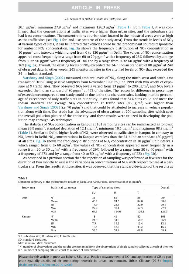
The spatial distribution of NO2 concentration in Kanpur is shown in Fig. 5a. In comparison to Delhi,Kanpur experienced less pronounced levels of pollution. Similar to Delhi, Kanpur had higher pollutionlevels near roadsides and industrial areas. Due to large commercial activities and more traffic conges-tions taking place in the city central area, this area could be considered as one of the hotspots of NO2

concentrations. The trends of spatial distributions of NO2 levels in this study were quite similar to thelevels, measured at a few locations through active sampling by our team members at CPCB (CPCB,2004). Fig. 5b shows the spatial distribution of NO2 that represented the probability to exceed40 lg/m3 concentrations in a locality. From Fig. 5b, it could be inferred that 50% area in Kanpur hadhigher chance with probability of 0.9 to exceed the annual Indian standard.

3.3. Proposing monitoring network for sampling sites

To examine the fact that control of NO2 can lead to reduce levels of other pollutants, we performeda linear correlation analysis between particulate matter with aerodynamic diameter 610 lm (PM10)and NO2 for 15 days average data during 2004 at national air quality sites that were maintained byour team members at CPCB in Delhi and Kanpur. As our passive sampling measurement was under-taken during February-March, 2004, we considered the observational data during these two monthsfrom national air quality sites for correlation analysis. The PM sampling was carried out using highvolume respirable dust sampler (APM-460 RDS, Envirotech, Delhi), which was equipped with acyclone to provide separation of PM10 particles with sharper cutoff (D50 at 10 lm) from the coarserparticles by centrifugal forces. When the suspended particles in air were drawn through the sampler,non-respirable particles (NRP) in air fell into the cyclone’s conical hopper and got collected in thecyclonic dust cup. The fine dust comprising the respirable fraction (PM10) passed through the cycloneand gets collected on the 20 � 25 cm Glass Microfibre Filter (GFF; Whatman grade). The sampling flowrate was maintained between 0.8 and 1.2 m3/min. The GFF filters and dust cups were pre-conditionedand post-conditioned at temperature �22 �C and RH �40% with controlled desiccators in the roommeant for conditioning for 24-hr. PM10 mass concentration (lg/m3) was determined gravimetricallyby the difference in mass of GFF after and before sampling (lg) divided by the volume of sampledair (m3). In a similar way to gravimetric method of PM10, the concentration of NRP was determinedfrom mass difference of respective dust cup after and before sampling and the volume of sampledair. The total suspended particle (TSP) concentration was calculated as the sum of PM10 collectedon the filter and NRP collected in the dust cup. In this study, we used the measurement data of

cite this article in press as: Behera, S.N., et al. Passive measurement of NO2 and application of GIS to gen-spatially-distributed air monitoring network in urban environment. Urban Climate (2015), http://.org/10.1016/j.uclim.2014.12.003

Fig. 4. Spatial distribution NO2 in Delhi: (a) map showing NO2 concentration in lg/m3, and (b) map showing possibility to pass40 lg/m3.

S.N. Behera et al. / Urban Climate xxx (2015) xxx–xxx 11

PM10 for interpretation. NO2 was measured by sampling through an absorbing solution in midget imp-inger system (connected in APM-460 RDS) followed by colorimetric method in the laboratory.

The number of national air quality sites being nine and six in Delhi and Kanpur, the pairs for linearcorrelation analysis were: n = 9 � 4 = 36 in Delhi and n = 6 � 4 = 24 in Kanpur. Fig. 6a and b shows the

Please cite this article in press as: Behera, S.N., et al. Passive measurement of NO2 and application of GIS to gen-erate spatially-distributed air monitoring network in urban environment. Urban Climate (2015), http://dx.doi.org/10.1016/j.uclim.2014.12.003

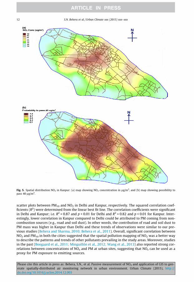
Fig. 5. Spatial distribution NO2 in Kanpur: (a) map showing NO2 concentration in lg/m3, and (b) map showing possibility topass 40 lg/m3.

12 S.N. Behera et al. / Urban Climate xxx (2015) xxx–xxx

scatter plots between PM10 and NO2 in Delhi and Kanpur, respectively. The squared correlation coef-ficients (R2) were determined from the linear best fit line. The correlation coefficients were significantin Delhi and Kanpur; i.e. R2 = 0.87 and p < 0.01 for Delhi and R2 = 0.82 and p < 0.01 for Kanpur. Inter-estingly, lower correlation in Kanpur compared to Delhi could be attributed to PM coming from non-combustion sources (e.g., road and soil dust). In other words, the contribution of road and soil dust toPM mass was higher in Kanpur than Delhi and these trends of observations were similar to our pre-vious studies (Behera and Sharma, 2010; Behera et al., 2011). Overall, significant correlation betweenNO2 and PM10 in both the cities suggested that the spatial pollution mapping of NO2 was a better wayto describe the patterns and trends of other pollutants prevailing in the study areas. Moreover, studiesin the past (Boogaard et al., 2011; Minguillón et al., 2012; Wang et al., 2013) also reported strong cor-relations between concentrations of NOx and PM at urban sites, suggesting that NOx can be used as aproxy for PM exposure to emitting sources.

Please cite this article in press as: Behera, S.N., et al. Passive measurement of NO2 and application of GIS to gen-erate spatially-distributed air monitoring network in urban environment. Urban Climate (2015), http://dx.doi.org/10.1016/j.uclim.2014.12.003

Fig. 6. Scatter plots between NO2 and PM and linear correlation from the best-fit line: (a) in Delhi, and (b) in Kanpur.

S.N. Behera et al. / Urban Climate xxx (2015) xxx–xxx 13

In the decision making process to propose the locations and numbers of sampling sites in these twolarge cities, maps showing spatial distributions of NO2 were examined to assess the most vulnerableareas through identification of hot spots. As described in a previous section, the current situation oftraffic volume, congestion and commercial activities were considered in addition to identifying thehotspots. In other words, the hotspots having higher probability of exceedance of critical thresholdvalue of 40 lg/m3 on NO2 concentration and with more traffic congestion were highly sensitive tohuman health risk due to more exposure of pollution. This should be noted that the sequence of plansfor making a proposal on location of monitoring sites was within the guidelines of EEA (1999). Hence,after identifying the critical areas, survey results on long-term meteorology, demographic patterns,and distribution of emitting sources were taken into account during the exercise in locating the sam-pling sites. It was observed that most populated districts in Delhi were (in decreasing order) as fol-lows: Northeast, Central, East, North and West. The site classifications were based on theconvention of three types; i.e. traffic, urban and suburban. The purpose for choosing suburban sitewas to get the background concentration and assess the effects of city pollution on the surroundingareas under downwind conditions.

Fig. 7a shows the locations of existing monitoring sites of national ambient air quality study main-tained by CPCB team during 2003–04. During decision making process, the existing sites of CPCB wereexamined for their suitability on the aspect whether to retain or reject. From this map, it was clear thatthe areas labelled with red color were extremely polluted and termed as hotspots for NO2 pollution.

Please cite this article in press as: Behera, S.N., et al. Passive measurement of NO2 and application of GIS to gen-erate spatially-distributed air monitoring network in urban environment. Urban Climate (2015), http://dx.doi.org/10.1016/j.uclim.2014.12.003

14 S.N. Behera et al. / Urban Climate xxx (2015) xxx–xxx

Based on source characteristics and population density, it was assessed that locating two traffic andthree urban monitoring sites would be more appropriate to present the data at such a highly pollutedarea of the city. The use of prevailing meteorology became paramount during finalization of samplinglocation of suburban sites. From the meteorological data during 2003–04, it was observed that thedirections of prevailing wind in Delhi were North to Northwest and East to Southeast. Therefore, allo-cating suburban sites at SE and NW would fulfil the purpose to represent the sites of background and

Fig. 7. Sampling network in spatial distribution map of Delhi: (a) existing NAMP sites, and (b) proposed monitoring sites.

Please cite this article in press as: Behera, S.N., et al. Passive measurement of NO2 and application of GIS to gen-erate spatially-distributed air monitoring network in urban environment. Urban Climate (2015), http://dx.doi.org/10.1016/j.uclim.2014.12.003

S.N. Behera et al. / Urban Climate xxx (2015) xxx–xxx 15

effects on city pollution flux on suburban region. For example under NW wind, NW suburban sitewould give background level characteristic of air in Delhi and SE suburban site would give levels ofpollution coming from city centre after photochemical transformation, where ozone (O3) levels areexpected to be the highest. This should be noted that during allocation of sampling sites, the trendsin levels of ambient O3 must be considered as the role of ambient O3 is very important in the atmo-spheric chemistry. From the observations of previous studies (Mavroidis and Ilia, 2012; Banan et al.,2013), it was believed that higher levels of O3 prevailing in the suburban regions could undergo trans-portation to reach the city area and would play significant role in atmospheric chemistry the city area.Therefore, as a future scope of work, it could be recommended that levels of tropospheric O3 at sub-urban regions should be monitored regularly. Fig. 7b shows the possible locations of automated sitesto be included in our proposed monitoring network in Delhi. In the decision making process for pro-posal of sampling sites, we considered to retain six sampling sites of national ambient air quality sitesand proposed nine more sites (total fifteen). Overall, these sites would present a complete pollutionscenario and the potential for population exposure to pollution over the city.

The prevailing wind direction in Kanpur was northwest to southeast. Approaches similar to Delhiwere adopted for decision making process on proposal of sampling sites (traffic, urban and suburban)in Kanpur for a monitoring network. Fig. 8 shows the proposed locations of the sampling sites. Twosuburban sites were proposed to represent both upwind and downwind characteristics of pollutionin the city. One sampling site was identified to account for industrial emissions (marked as industrialsite in Fig. 8 and it was urban type in nature). Based on the locations of hotspots, source characteristicsand population density, it was decided to allocate one traffic and two urban sampling sites in the citycentral area. Other possible locations were considered for traffic and urban set up at moderate pollu-tion levels. In addition, one urban sampling site was proposed to account for the second critical area inthe east side of Kanpur. Retaining location of the industrial site, traffic and urban sites in the city cen-tral area of the national ambient air quality study, we proposed five additional sampling sites. Hence,it appeared that by allocating eight sampling sites in Kanpur, overall pollution scenario of the citycould be represented.

The future scope of the research on proposal of monitoring network for measurement of airpollutants in urban environment could be extended through parallel measurement of O3, SO2 andNH3 along with NO2 using passive samplers. With the measurement results of these precursor gases,the trends of atmospheric chemistry could be studied in distinctions with time and space. The findingsfrom the role of atmospheric chemistry of these precursor gases on formation of secondary compo-nents of PM would improve the decision making process on allocation of sampling sites.

Fig. 8. Sampling network in spatial distribution map of Kanpur: proposed monitoring sites.

Please cite this article in press as: Behera, S.N., et al. Passive measurement of NO2 and application of GIS to gen-erate spatially-distributed air monitoring network in urban environment. Urban Climate (2015), http://dx.doi.org/10.1016/j.uclim.2014.12.003

16 S.N. Behera et al. / Urban Climate xxx (2015) xxx–xxx

4. Conclusions

The present study demonstrates a systematic approach that describes the application of GISthrough Kriging interpolation method with the experimental outcomes of passive sampling to gener-ate spatially-resolved maps of NO2 levels. These results were used in identification of monitoring sitesrequired for continuous long-term measurement in two megacities of India (Delhi and Kanpur). Pas-sive sampling of NO2 was conducted at 204 and 101 sampling locations in Delhi and Kanpur, respec-tively. It was observed that Delhi and Kanpur experienced an average NO2 concentration of68.6 ± 20.1 lg/m3and 36.9 ± 12.1 lg/m3, respectively. A significant correlation between NO2 andPM10 in both cities suggests that the spatial pollution mapping of NO2 is good enough to describethe patterns and trends that are also valid for other pollutants. On the basis of survey results on emis-sion activities, meteorology and guidelines for site selection criteria with its characteristics (urban,traffic and suburban types), this study proposes that Delhi and Kanpur need fifteen and eight numberof sampling sites to represent the complete pollution scenario. The study emphasizes on location ofsuburban or background sampling sites for overall assessment on the pollution levels and their expo-sure to the existing population.

Acknowledgements

This research study was part of the project ‘‘Air Quality Monitoring in India’’, conducted in collab-orative efforts among Central Pollution Control Board, Delhi, ETI group, BURGEAP, France, and IndianInstitute of Technology, Kanpur. We also thank two anonymous reviewers for their valuable com-ments that helped for substantial improvement of this article.

References

Agarwal, R., Jayaraman, G., Anand, S., Marimuthu, P., 2006. Assessing respiratory morbidity through pollution status andmeteorological conditions for Delhi. Environ. Monit. Assess. 114 (1–3), 489–504.

Ahmad, S.S., Biiker, P., Emberson, L., Shabbir, R., 2011. Monitoring nitrogen dioxide levels in urban areas in Rawalpindi, Pakistan.Water Air Soil Poll. 220, 141–150.

Allegrini, I., Costabile, F., 2002. A new approach for monitoring atmospheric pollution in urban environment, Global Conferenceon Building a Sustainable World, San-Paolo, Brasil.

Baldasano, J.M., Valera, E., Jiménez, P., 2003. Air quality data from large cities. Sci. Total Environ. 307 (1), 141–165.Banan, N., Latif, M.T., Juneng, L., Ahamad, F., 2013. Characteristics of surface ozone concentrations at stations with different

backgrounds in the Malaysian Peninsula. Aerosol Air Qual. Res. 13, 1090–1106.Bartkow, M.E., Booij, K., Kennedy, K.E., Muller, J.F., Hawker, D.W., 2005. Passive air sampling theory for semi-volatile organic

compounds. Chemosphere 60, 170–176.Behera, S.N., Sharma, M., 2010. Reconstructing primary and secondary components of PM2.5 composition for an urban

atmosphere. Aerosol Sci. Technol. 44 (11), 983–992.Behera, S.N., Sharma, M., Dikshit, O., Shukla, S.P., 2011. GIS-based emission inventory, dispersion modeling, and assessment for

source contributions of particulate matter in an urban environment. Water Air Soil Poll. 218, 423–436.Behera, S.N., Sharma, M., Nayak, P., Shukla, S.P., Gargava, P., 2014. An approach for evaluation of proposed air pollution control

strategy to reduce levels of nitrogen oxides in an urban environment. J. Environ. Plann. Manage. 57, 467–494.Bhati, K.R., 2000. In: Bose, R.K., Sundar, S., Nesamani, K.S. (Eds.), Performance of On-road Vehicles and Emission Standards in

Clearing the Air – Better Vehicles, Better Fuels. Tata Energy Research Institute, Delhi, pp. 49–54.Boogaard, H., Kos, G., Weijers, E.P., Janssen, N.A., Fischer, P.H., van der Zee, S.C., de Hartog, J.J., Hoek, G., 2011. Contrast in air

pollution components between major streets and background locations: particulate matter mass, black carbon, elementalcomposition, nitrogen oxide and ultrafine particle number. Atmos. Environ. 45 (3), 650–658.

Bootdee, S., Chalemrom, P., Chantara, S., 2012. Validation and field application of tailor-made nitrogen dioxide passive samplers.Int. J. Environ. Sci. Technol. 9, 515–526.

Briggs, D.J., Collins, S., Elliott, P., Fischer, P., Kingham, S., Lebret, E., Pryl, K., Reeuwijk, H.V., Smallbone, K., Veen, A.V.D., 1997.Mapping urban air pollution using GIS: a regression based approach. Int. J. Geogr. Inf. Sci. 11, 699–718.

Briggs, D.J., de Hoogh, C., Gulliver, J., Wills, J., Elliott, P., Kinghamc, S., Smallbone, K., 2000. A regression-based method formapping traffic-related air pollution: application and testing in four contrasting urban environments. Sci. Total Environ.253, 151–167.

Campbell, G.W., Stedman, J.R., Stevenson, K., 1994. A survey of nitrogen dioxide concentrations in the United Kingdom usingdiffusion tubes July–December 1991. Atmos. Environ. 28 (3), 477–487.

Cohen, A.J., Anderson, H.R., Ostro, B., Pandey, K.D., Krzyzanowski, M., Kuenzli, N., Gutschmidt, K., Pope, C.A., Romieu, I., Samet,J.M., Smith, K., et al, 2004. Mortality impacts of urban air pollution. In: Ezzati, m. (Ed.), Comparative Quantification of HealthRisks: Global and Regional Burden of Disease Attributable to Selected Major Risk Factors. World Health Organization,Geneva, pp. 1353–1434.

CPCB, 2004. National Ambient Air Quality Status 2004, Central Pollution Control Board, Delhi, India.

Please cite this article in press as: Behera, S.N., et al. Passive measurement of NO2 and application of GIS to gen-erate spatially-distributed air monitoring network in urban environment. Urban Climate (2015), http://dx.doi.org/10.1016/j.uclim.2014.12.003

S.N. Behera et al. / Urban Climate xxx (2015) xxx–xxx 17

Cruz, L.P.S., Campos, V.P., Silva, A.M.C., Tavares, T.M., 2004. A field evaluation of a SO2 passive sampler in tropical industrial andurban air. Atmos. Environ. 38, 6425–6429.

EEA, 1999. Criteria for EUROAIRNET – The EEA Air Quality Monitoring and Information Network. Technical Report No. 12.European Environment Agency, Copenhagen.

Ferm, M., Svanberg, P.-A., 1998. Cost-efficient techniques for urban- and background measurements of SO2 and NO2. Atmos.Environ. 32, 1377–1381.

Garg, A., Shukla, P.R., Kapshe, M., 2006. The sectoral trends of multigas emissions inventory of India. Atmos. Environ. 40, 4608–4620.

Gokhale, S., Raokhande, N., 2008. Performance evaluation of air quality models for predicting PM10 and PM2.5 concentrations aturban traffic intersection during winter period. Sci. Total Environ. 394 (1), 9–24.

Haas, T.C., 1992. Redesigning continental-scale monitoring networks. Atmos. Environ. 26A, 3323–3333.Hadad, K., Safavi, A., Tahon, R., 2005. Air pollution assessment in Shiraz by passive sampling techniques, Iran. J. Sci. Technol. 29

(A3), 471.Hansen, T.S., Kruse, M., Nissen, H., Glasius, M., Lohse, C., 2001. Measurements of nitrogen dioxide in Greenland using Palmes

diffusion tubes. J. Environ. Monitor. 3, 139–145.Harner, T., Shoeib, M., Diamond, M., Stern, G., Rosenberg, B., 2004. Using passive air samplers to assess urban–rural trends for

persistent organic pollutants. 1. polychlorinated biphenyls and organochlorine pesticides. Environ. Sci. Technol. 38, 4474–4483.

Jackson, M.M., 2005. Roadside concentration of gaseous and particulate matter pollutants and risk assessment in Dar-es-Salaam,Tanzania. Environ. Monit. Assess. 104 (1–3), 385–407.

Janssen, N.A., van Vliet, P.H., Aarts, F., Harssema, H., Brunekreef, B., 2001. Assessment of exposure to traffic related air pollutionof children attending schools near motorways. Atmos. Environ. 35 (22), 3875–3884.

Johnston, K., Ver Hoef, J.M., Krivoruchko, K., Lucas, N., 2001. Using ArcGIS Geostatistical Analyst, vol. 300. Esri, Redlands.Kampa, M., Castanas, E., 2008. Human health effects of air pollution. Environ. Pollut. 151 (2), 362–367.Klimont, Z., Cofala, J., Xing, J., Wei, W., Zhang, C., Wang, S., Kejun, J., Bhandari, P., Mathur, R., Purohit, P., Rafaj, P., Chambers, A.,

Amann, M., 2009. Projections of SO2, NOx and carbonaceous aerosols emissions in Asia. Tellus Ser. B 61, 602–617.Krochmal, D., Kalina, A., 1997. Measurements of nitrogen dioxide and sulphur dioxide concentrations in urban and rural areas of

Poland using a passive sampling method. Environ. Pollut. 96, 401–140.Lal, S., Patil, R.S., 2001. Monitoring of atmospheric behaviour of NOx from vehicular traffic. Environ. Monit. Assess. 68 (1), 37–50.Lawrence, M.G., Butler, T.M., Steinkamp, J., Gurjar, B.R., Lelieveld, J., 2007. Regional pollution potentials of megacities and other

major population centers. Atmos. Chem. Phys. 7 (14), 3969–3987.Lewne, M., Cyrys, J., Meliefste, K., Hoek, G., Brauer, M., Fischer, P., et al, 2004. Spatial variation in nitrogen dioxide in three

European areas. Sci. Total Environ. 332, 217–230.Liu, L.J.S., Rossini, A., Koutrakis, P., 1995. Development of co-Kriging models to predict 1- and 12-hour ozone concentrations in

Toronto. Epidemiology 6, S69.Lozano, A., Usero, J., Vanderlinden, E., Raez, J., Contreras, J., Navarrete, B., 2009. Air quality monitoring network design to control

nitrogen dioxide and ozone, applied in Malaga,Spain. Microchem. J. 93, 164–172.Mallik, C., Lal, S., 2014. Seasonal characteristics of SO2, NO2, and CO emissions in and around the Indo-Gangetic Plain. Environ.

Monit. Assess. 186 (2), 1295–1310.Maruo, Y.Y., Ogawa, S., Ichino, T., Murao, N., Uchiyama, M., 2003. Measurement of local variations in atmospheric nitrogen

dioxide levels in Sapporo, Japan, using a new method with high spatial and high temporal resolution. Atmos. Environ. 37 (8),1065–1074.

Mavroidis, I., Ilia, M., 2012. Trends of NOx, NO2 and O3 concentrations at three different types of air quality monitoring stationsin Athens,Greece. Atmos. Environ. 63, 135–147.

Millstein, D.E., Harley, R.A., 2010. Effects of retrofitting emission control systems on in-use heavy diesel vehicles. Environ. Sci.Technol. 44 (13), 5042–5048.

Minguillón, M.C., Rivas, I., Aguilera, I., Alastuey, A., Moreno, T., Amato, F., Sunyer, J., Querol, X., 2012. Within-city contrasts in PMcomposition and sources and their relationship with nitrogen oxides. J. Environ. Monitor. 14 (10), 2718–2728.

Myers, D.E., 1994. Spatial interpolation: an overview. Geoderma 62, 17–28.Noll, K.E., Miller, T.L., Narco, J.E., Raufer, R.K., 1977. An objective air monitoring site selection methodology for large point

sources. Atmos. Environ. 11, 1051–1059.Oliver, M.A., Webster, R., 1990. Kriging: a method of interpolation for geographical information systems. Int. J. Geogr. Inf. Sci. 4,

313–332.Palmes, E.D., Gunnison, A.F., Dimatto, J., Tomezyk, C., 1976. Personal sampler for nitrogen dioxide. Am. Ind. Hyg. Assoc. J. 37,

570–577.Pucher, J., Peng, Z.R., Mittal, N., Zhu, Y., Korattyswaroopam, N., 2007. Urban transport trends and policies in China and India:

impacts of rapid economic growth. Transport rev. 27, 379–410.Ravindra, K., Sokhi, R., Van Grieken, R., 2008. Atmospheric polycyclic aromatic hydrocarbons: source attribution, emission

factors and regulation. Atmos. Environ. 42 (13), 2895–2921.RTO, 2006. Annual Report on Vehicles Status in Kanpur, Regional Transport Office, Kanpur, India.Salem, A.A., Soliman, A.A., El-Haty, A.I., 2009. Determination of nitrogen dioxide, sulfur dioxide, ozone and ammonia in ambient

air using the passive sampling method associated with ion chromatographic and potentiometric analyses. Air Qual. Atmos.Health 2, 133–145.

Schaug, J., Iversen, T., Pedersen, U., 1993. Comparison of measurements and model results for airborne sulphur and nitrogencomponents with Kriging. Atmos. Environ. 27A, 831–844.

Sharma, S.K., Mandal, T.K., Saxena, M., Sharma, A., Gautam, R., 2013. Source apportionment of PM10 by using positive matrixfactorization at an urban site of Delhi, India. Urban Clim.. http://dx.doi.org/10.1016/j.uclim.2013.11.002.

Shoeib, M., Harner, T., 2002. Characterization and comparison of three passive air samplers for persistent organic pollutants.Environ. Sci. Technol. 36, 4142–4151.

Please cite this article in press as: Behera, S.N., et al. Passive measurement of NO2 and application of GIS to gen-erate spatially-distributed air monitoring network in urban environment. Urban Climate (2015), http://dx.doi.org/10.1016/j.uclim.2014.12.003

18 S.N. Behera et al. / Urban Climate xxx (2015) xxx–xxx

Singh, D.P., Gadi, R., Mandal, T.K., 2011. Characterization of particulate-bound polycyclic aromatic hydrocarbons and tracemetals composition of urban air in Delhi, India. Atmos. Environ. 45 (40), 7653–7663.

Stock, Z.S., Russo, M.R., Butler, T.M., Archibald, A.T., Lawrence, M.G., Telford, P.J., Abraham, N.L., Pyle, J.A., 2013. Modelling theimpact of megacities on local, regional and global tropospheric ozone and the deposition of nitrogen species. Atmos. Chem.Phys. 13 (24), 12215–12231.

U.S. Environmental Protection Agency (US EPA), 1994. Photochemical Assessment Monitoring Stations (PAMS) ImplementationManual. Office of Air Quality Planning and Standards, Report No. EPA-454/B-93-051.

Varshney, C.K., Singh, A.P., 2002. Measurement of ambient concentration of NO2 in Delhi using passive diffusion tube sampler.Curr. Sci. India 83 (6), 731–735.

Varshney, C.K., Singh, A.P., 2003. Passive samplers for NOx monitoring. Environmentalist 23, 127–136.Vione, D., Maurino, V., Minero, C., Pelizzetti, E., Harrison, M.A., Olariu, R.I., Arsene, C., 2006. Photochemical reactions in the

tropospheric aqueous phase and on particulate matter. Chem. Soc. Rev. 35 (5), 441–453.Wang, M., Beelen, R., Basagana, X., Becker, T., Cesaroni, G., de Hoogh, K., et al, 2013. Evaluation of land use regression models for

NO2 and particulate matter in 20 European study areas: the ESCAPE project. Environ. Sci. Technol. 47 (9), 4357–4364.

Please cite this article in press as: Behera, S.N., et al. Passive measurement of NO2 and application of GIS to gen-erate spatially-distributed air monitoring network in urban environment. Urban Climate (2015), http://dx.doi.org/10.1016/j.uclim.2014.12.003