Analysis of Complex Survey Data in Stata

Isabel CañetteSenior Statistician

StataCorp LP

2010 Mexican Stata Users Group meetingApril 29, 2010

Introduction

I Surveys are aimed to collect information to studycharacteristics on a fixed population

I Surveys (as opposed to census) are usually performed to cutcosts and time resources

I For the same reasons, researchers may opt for complex surveydesigns, as opposed to simple random samples (SRS)

I In some situations, SRS may be impossible due to lack of a listwith all the individuals.

Stata approach to survey data

In Stata, we separate the stage of the declaration of the designfrom the estimation stage. Once the design is declared (svyset), itwill be automatically taken into account every time we use the svyprefix.

If for i.i.d data we write:

regressproportion

Then, for survey data we write:

svy: regresssvy: proportion

Survey data characteristics

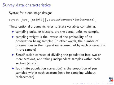
Syntax for a one-stage design:

svyset[psu

] [weight

] [, strata(varname ) fpc(varname )

]These optional arguments refer to Stata variables containing:

I sampling units, or clusters, are the actual units we sample.I sampling weight is the inverse of the probability of an

observation being sampled (in other words, the number ofobservations in the population represented by each observationin the sample)

I Stratification consists of dividing the population into two ormore sections, and taking independent samples within eachsection (strata).

I fpc (finite population correction) is the proportion of psusampled within each stratum (only for sampling withoutreplacement)

Using svyset for a SRS

If we have a SRS (without replacement), we will usually consider itas “standard” data. There are, however, cases in which we maywant to use svyset. We’ll use this setting to illustrate the use offpc and weight.

Using svyset for a SRS

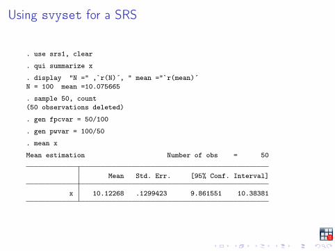
. use srs1, clear

. qui summarize x

. display "N =" ,`r(N)´, " mean ="`r(mean)´N = 100 mean =10.075665

. sample 50, count(50 observations deleted)

. gen fpcvar = 50/100

. gen pwvar = 100/50

. mean x

Mean estimation Number of obs = 50

Mean Std. Err. [95% Conf. Interval]

x 10.12268 .1299423 9.861551 10.38381

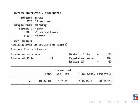
. svyset [pw=pwvar], fpc(fpcvar)

pweight: pwvarVCE: linearized

Single unit: missingStrata 1: <one>

SU 1: <observations>FPC 1: fpcvar

. svy: mean x(running mean on estimation sample)

Survey: Mean estimation

Number of strata = 1 Number of obs = 50Number of PSUs = 50 Population size = 100

Design df = 49

LinearizedMean Std. Err. [95% Conf. Interval]

x 10.04064 .1075293 9.824552 10.25673

Simple design with two strata

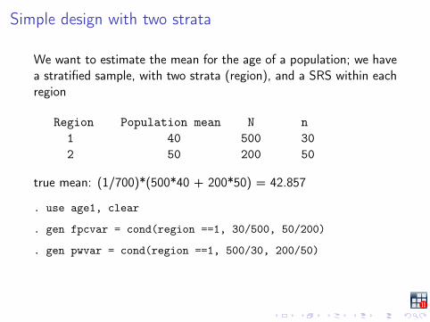
We want to estimate the mean for the age of a population; we havea stratified sample, with two strata (region), and a SRS within eachregion

Region Population mean N n1 40 500 302 50 200 50

true mean: (1/700)*(500*40 + 200*50) = 42.857

. use age1, clear

. gen fpcvar = cond(region ==1, 30/500, 50/200)

. gen pwvar = cond(region ==1, 500/30, 200/50)

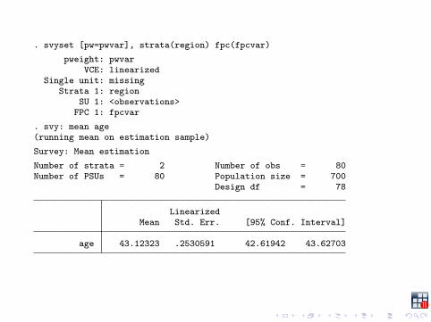
. svyset [pw=pwvar], strata(region) fpc(fpcvar)pweight: pwvar

VCE: linearizedSingle unit: missing

Strata 1: regionSU 1: <observations>

FPC 1: fpcvar. svy: mean age(running mean on estimation sample)Survey: Mean estimationNumber of strata = 2 Number of obs = 80Number of PSUs = 80 Population size = 700

Design df = 78

LinearizedMean Std. Err. [95% Conf. Interval]

age 43.12323 .2530591 42.61942 43.62703

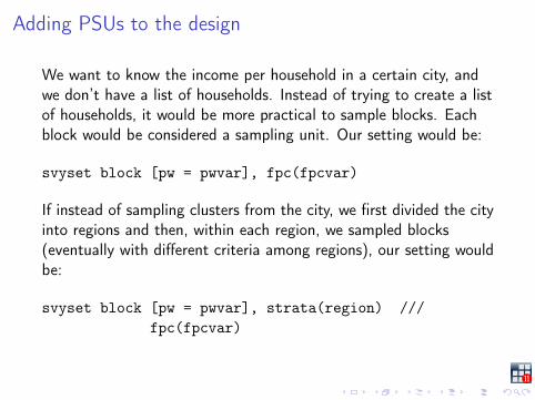
Adding PSUs to the design

We want to know the income per household in a certain city, andwe don’t have a list of households. Instead of trying to create a listof households, it would be more practical to sample blocks. Eachblock would be considered a sampling unit. Our setting would be:

svyset block [pw = pwvar], fpc(fpcvar)

If instead of sampling clusters from the city, we first divided the cityinto regions and then, within each region, we sampled blocks(eventually with different criteria among regions), our setting wouldbe:

svyset block [pw = pwvar], strata(region) ///fpc(fpcvar)

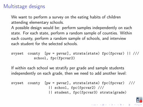
Multistage designs

We want to perform a survey on the eating habits of childrenattending elementary schools.A possible design would be: perform samples independently on eachstate. For each state, perform a random sample of counties. Withineach county, perform a random sample of schools, and intervieweach student for the selected schools.

svyset county [pw = pwvar], strata(state) fpc(fpcvar) || ///school, fpc(fpcvar2)

If within each school we stratify per grade and sample studentsindependently on each grade, then we need to add another level:

svyset county [pw = pwvar], strata(state) fpc(fpcvar) ///|| school, fpc(fpcvar2) ///|| student, fpc(fpcvar3) strata(grade)

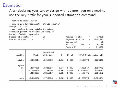
EstimationAfter declaring your survey design with svyset, you only need touse the svy prefix for your supported estimation command.. webuse nhanes2, clear. svyset psu [pw=finalwgt], strata(strata)(output omitted). svy: probit highbp weight i.region(running probit on estimation sample)Survey: Probit regressionNumber of strata = 31 Number of obs = 10351Number of PSUs = 62 Population size = 117157513

Design df = 31F( 4, 28) = 51.58Prob > F = 0.0000

Linearizedhighbp Coef. Std. Err. t P>|t| [95% Conf. Interval]

weight .0229814 .0016002 14.36 0.000 .0197178 .0262449

region2 -.1367888 .1321226 -1.04 0.309 -.4062547 .13267723 -.0568238 .1284056 -0.44 0.661 -.3187087 .20506114 -.1563827 .1255029 -1.25 0.222 -.4123475 .0995822

_cons -2.889106 .1712036 -16.88 0.000 -3.238278 -2.539934

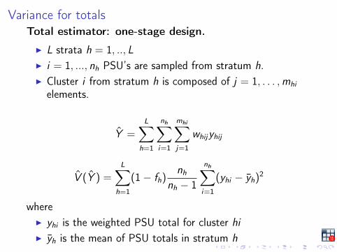
Variance for totalsTotal estimator: one-stage design.

I L strata h = 1, .., LI i = 1, ..., nh PSU’s are sampled from stratum h.I Cluster i from stratum h is composed of j = 1, . . . , mhi

elements.

Y =L∑

h=1

nh∑i=1

mhi∑j=1

whijyhij

V (Y ) =L∑

h=1

(1 − fh)nh

nh − 1

nh∑i=1

(yhi − yh)2

whereI yhi is the weighted PSU total for cluster hiI yh is the mean of PSU totals in stratum h

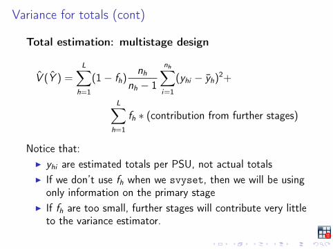
Variance for totals (cont)

Total estimation: multistage design

V (Y ) =L∑

h=1

(1 − fh)nh

nh − 1

nh∑i=1

(yhi − yh)2+

L∑h=1

fh ∗ (contribution from further stages)

Notice that:I yhi are estimated totals per PSU, not actual totalsI If we don’t use fh when we svyset, then we will be using

only information on the primary stageI If fh are too small, further stages will contribute very little

to the variance estimator.

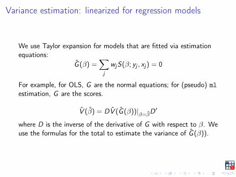
Variance estimation: linearized for regression models

We use Taylor expansion for models that are fitted via estimationequations:

G (β) =∑

j

wjS(β; yj , xj) = 0

For example, for OLS, G are the normal equations; for (pseudo) mlestimation, G are the scores.

V (β) = DV (G (β))|β=βD ′

where D is the inverse of the derivative of G with respect to β. Weuse the formulas for the total to estimate the variance of G (β)).

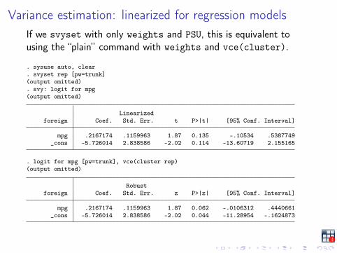
Variance estimation: linearized for regression modelsIf we svyset with only weights and PSU, this is equivalent tousing the “plain” command with weights and vce(cluster).

. sysuse auto, clear

. svyset rep [pw=trunk](output omitted). svy: logit for mpg(output omitted)

Linearizedforeign Coef. Std. Err. t P>|t| [95% Conf. Interval]

mpg .2167174 .1159963 1.87 0.135 -.10534 .5387749_cons -5.726014 2.838586 -2.02 0.114 -13.60719 2.155165

. logit for mpg [pw=trunk], vce(cluster rep)(output omitted)

Robustforeign Coef. Std. Err. z P>|z| [95% Conf. Interval]

mpg .2167174 .1159963 1.87 0.062 -.0106312 .4440661_cons -5.726014 2.838586 -2.02 0.044 -11.28954 -.1624873

Replication-based methods

I Allow us to compute variance estimates without having thewhole design information

I They use a set of variables containing weights: estimation isperformed using each variable weight, and all those results areused to compute the variance

I Different methods differ on how weights are computed, andtherefore on the formula used to compute the variance.

I Currently, we have two replication-based methods: jackknifeand brr (balanced repeated replications).

I In the near future, we will also have bootstrap and sdr(successive difference replications).

The bootstrap

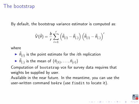
By default, the bootstrap variance estimator is computed as:

V (θ) =br

r∑i=1

(θ(i) − θ(.)

) (θ(i) − θ(.)

)′

whereI θ(i) is the point estimate for the ith replicationI θ(.) is the mean of {θ(1), . . . , θ(r)}

Computation of bootstrap vce for survey data requires thatweights be supplied by user.Available in the near future. In the meantime, you can use theuser-written command bs4rw (use findit to locate it).

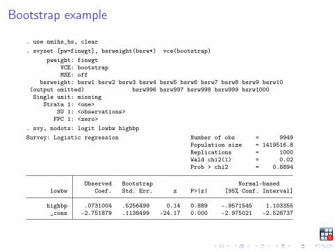
Bootstrap example

. use nmihs_bs, clear

. svyset [pw=finwgt], bsrweight(bsrw*) vce(bootstrap)pweight: finwgt

VCE: bootstrapMSE: off

bsrweight: bsrw1 bsrw2 bsrw3 bsrw4 bsrw5 bsrw6 bsrw7 bsrw8 bsrw9 bsrw10(output omitted) bsrw996 bsrw997 bsrw998 bsrw999 bsrw1000Single unit: missing

Strata 1: <one>SU 1: <observations>

FPC 1: <zero>. svy, nodots: logit lowbw highbpSurvey: Logistic regression Number of obs = 9949

Population size = 1419516.8Replications = 1000Wald chi2(1) = 0.02Prob > chi2 = 0.8894

Observed Bootstrap Normal-basedlowbw Coef. Std. Err. z P>|z| [95% Conf. Interval]

highbp .0731004 .5256499 0.14 0.889 -.9571545 1.103355_cons -2.751879 .1138499 -24.17 0.000 -2.975021 -2.528737

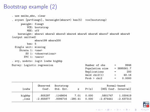
Bootstrap example (2). use nmihs_mbs, clear. svyset [pw=finwgt], bsrweight(mbsrw*) bsn(5) vce(bootstrap)

pweight: finwgtVCE: bootstrapMSE: off

bsrweight: mbsrw1 mbsrw2 mbsrw3 mbsrw4 mbsrw5 mbsrw6 mbsrw7 mbsrw8 mbsrw9(output omitted)

mbsrw199 mbsrw200bsn: 5

Single unit: missingStrata 1: <one>

SU 1: <observations>FPC 1: <zero>

. svy, nodots: logit lowbw highbpSurvey: Logistic regression Number of obs = 9946

Population size = 3895561.7Replications = 200Wald chi2(1) = 49.16Prob > chi2 = 0.0000

Observed Bootstrap Normal-basedlowbw Coef. Std. Err. z P>|z| [95% Conf. Interval]

highbp .805297 .1148604 7.01 0.000 .5801747 1.030419_cons -2.655877 .0094716 -280.41 0.000 -2.674441 -2.637313

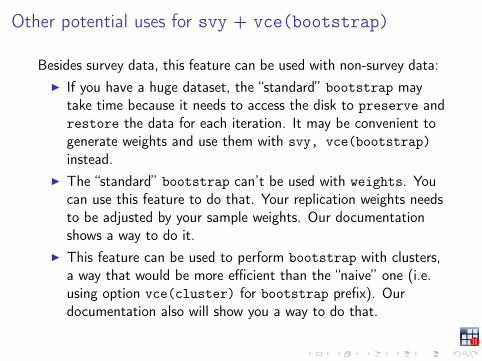
Other potential uses for svy + vce(bootstrap)

Besides survey data, this feature can be used with non-survey data:I If you have a huge dataset, the “standard” bootstrap may

take time because it needs to access the disk to preserve andrestore the data for each iteration. It may be convenient togenerate weights and use them with svy, vce(bootstrap)instead.

I The “standard” bootstrap can’t be used with weights. Youcan use this feature to do that. Your replication weights needsto be adjusted by your sample weights. Our documentationshows a way to do it.

I This feature can be used to perform bootstrap with clusters,a way that would be more efficient than the “naive” one (i.e.using option vce(cluster) for bootstrap prefix). Ourdocumentation also will show you a way to do that.

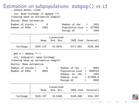
Estimation on subpopulations: subpop() vs if. webuse nmihs, clear. svy: mean birthwgt if agegrp ==1(running mean on estimation sample)Survey: Mean estimationNumber of strata = 6 Number of obs = 1652Number of PSUs = 1652 Population size = 477969

Design df = 1646

LinearizedMean Std. Err. [95% Conf. Interval]

birthwgt 3205.137 16.9503 3171.891 3238.384

. gen u = agegrp == 1

. svy, subpop(u): mean birthwgt(running mean on estimation sample)Survey: Mean estimationNumber of strata = 6 Number of obs = 9952Number of PSUs = 9952 Population size = 3898763

Subpop. no. obs = 1652Subpop. size = 477968.6Design df = 9946

LinearizedMean Std. Err. [95% Conf. Interval]

birthwgt 3205.137 18.5948 3168.688 3241.587

Estimation on subpopulations: Remarks

Unless you have a very good reason to do the opposite, always usesubpop() (not if/in) when working with svy data.

I if/in restricts the data to the subset of observations thatsatisfy the condition, and performs the estimation as if it werethe whole sample from a known “population”.

I It underestimates the variance, because it ignores the fact thatour sample was taken from the whole population (not from thesubset with the if condition in the population), and then werestricted the analysis to the observations that happened to bein the subset.

Postestimation commands

Most post-estimation commands are also available for survey data:lincom, nlcom, predict, predictnl, test, testnl, work thesame way as for “standard” estimations.When performing a Wald test after svy estimation, degrees offeedom for test are adjusted according to the survey design.The command test is particularly important for survey data, wherelikelihood-based commands (like lrtest) are not valid.

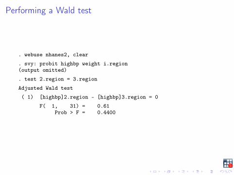
Performing a Wald test

. webuse nhanes2, clear

. svy: probit highbp weight i.region(output omitted)

. test 2.region = 3.region

Adjusted Wald test

( 1) [highbp]2.region - [highbp]3.region = 0

F( 1, 31) = 0.61Prob > F = 0.4400

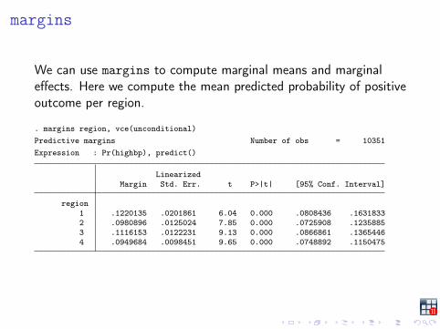
margins

We can use margins to compute marginal means and marginaleffects. Here we compute the mean predicted probability of positiveoutcome per region.

. margins region, vce(unconditional)Predictive margins Number of obs = 10351Expression : Pr(highbp), predict()

LinearizedMargin Std. Err. t P>|t| [95% Conf. Interval]

region1 .1220135 .0201861 6.04 0.000 .0808436 .16318332 .0980896 .0125024 7.85 0.000 .0725908 .12358853 .1116153 .0122231 9.13 0.000 .0866861 .13654464 .0949684 .0098451 9.65 0.000 .0748892 .1150475