Using Stata for Survey Data Analysis - Food Security Portal training... · Using Stata for Survey...
63
Using Stata for Survey Data Analysis Nicholas Minot International Food Policy Research Institute Washington, DC, USA 30 November 2009
Transcript of Using Stata for Survey Data Analysis - Food Security Portal training... · Using Stata for Survey...
Using Stata for Survey Data Analysis
Nicholas Minot
International Food Policy Research Institute
Washington, DC, USA
30 November 2009

Minot Using Stata for Survey Data Analysis
Table of Contents
SECTION 1: INTRODUCTION TO TRAINING GUIDE ............................................................... 1 Background ......................................................................................................................................... 1 Objectives ........................................................................................................................................... 1 Course requirements ........................................................................................................................... 1 Organization of the course .................................................................................................................. 1
SECTION 2: REVIEW OF SURVEY DATA CONCEPTS ............................................................ 3 List of useful terms ............................................................................................................................. 3 Structure of BLSS data files ............................................................................................................... 4
SECTION 3: INTRODUCTION TO STATA .................................................................................. 5 Menu bar ............................................................................................................................................. 5 Tool bar ............................................................................................................................................... 6 Stata windows ..................................................................................................................................... 6
SECTION 4: EXPLORING DATA FILES ...................................................................................... 9 cd ......................................................................................................................................................... 9 clear ..................................................................................................................................................... 9 use ....................................................................................................................................................... 9 describe ............................................................................................................................................. 10 list ...................................................................................................................................................... 10 summarize ......................................................................................................................................... 11 tabulate, tab1, tab2 ............................................................................................................................ 12 bysort prefix ...................................................................................................................................... 14 save ................................................................................................................................................... 14 in ....................................................................................................................................................... 15 help .................................................................................................................................................... 15 set ...................................................................................................................................................... 15 Exercises for exploring the BLSS ..................................................................................................... 15
SECTION 5: STORING COMMANDS AND OUTPUT .............................................................. 17 Using the Do-file Editor .................................................................................................................... 17 Saving the output .............................................................................................................................. 18 Using Stata output ............................................................................................................................. 20 Exercises for saving commands and output ...................................................................................... 21
SECTION 6: CREATING NEW VARIABLES AND ADDING LABELS ................................. 22 generate ............................................................................................................................................. 22 replace ............................................................................................................................................... 22 tabulate … generate .......................................................................................................................... 23 Using functions ................................................................................................................................. 26 recode ................................................................................................................................................ 26 xtile ................................................................................................................................................... 27 label variable ..................................................................................................................................... 28 label define ........................................................................................................................................ 28 label values........................................................................................................................................ 29 #delimit ............................................................................................................................................. 30 Exercises for creating variables and labels ....................................................................................... 31
Using Stata for Survey Data Analysis Minot
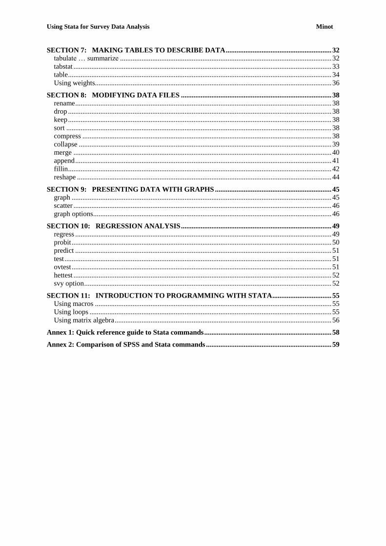
SECTION 7: MAKING TABLES TO DESCRIBE DATA ........................................................... 32 tabulate … summarize ...................................................................................................................... 32 tabstat ................................................................................................................................................ 33 table ................................................................................................................................................... 34 Using weights.................................................................................................................................... 36
SECTION 8: MODIFYING DATA FILES .................................................................................... 38 rename ............................................................................................................................................... 38 drop ................................................................................................................................................... 38 keep ................................................................................................................................................... 38 sort .................................................................................................................................................... 38 compress ........................................................................................................................................... 38 collapse ............................................................................................................................................. 39 merge ................................................................................................................................................ 40 append ............................................................................................................................................... 41 fillin ................................................................................................................................................... 42 reshape .............................................................................................................................................. 44
SECTION 9: PRESENTING DATA WITH GRAPHS ................................................................. 45 graph ................................................................................................................................................. 45 scatter ................................................................................................................................................ 46 graph options ..................................................................................................................................... 46
SECTION 10: REGRESSION ANALYSIS .................................................................................... 49 regress ............................................................................................................................................... 49 probit ................................................................................................................................................. 50 predict ............................................................................................................................................... 51 test ..................................................................................................................................................... 51 ovtest ................................................................................................................................................. 51 hettest ................................................................................................................................................ 52 svy option .......................................................................................................................................... 52
SECTION 11: INTRODUCTION TO PROGRAMMING WITH STATA ................................. 55 Using macros .................................................................................................................................... 55 Using loops ....................................................................................................................................... 55 Using matrix algebra ......................................................................................................................... 56
Annex 1: Quick reference guide to Stata commands ....................................................................... 58
Annex 2: Comparison of SPSS and Stata commands ...................................................................... 59


Using Stata for Survey Data Analysis Minot
Page 1
SECTION 1: INTRODUCTION TO TRAINING GUIDE
Background
This manual was prepared to be used as part of a one-week training course. Earlier versions of the
manual have been used in training courses in various countries. This manual describes how to use
Stata to store, describe, and analyze data. The emphasis is on the analysis of household survey data,
but Stata can be used with any database.
It should be noted that this course is not a lecture course, but rather it is a semi-structured hands-on
workshop in which trainees will use computers to learn different methods of analyzing data. Thus,
active participation of the trainees is expected and necessary to maximize the benefit from the
training.
The training modules focus on how to use computer software to implement a wide range of topics and
analytical methods. In order to cover this range of methods, the course cannot provide detailed
explanations of the all statistical methods themselves, so it is assumed that trainees have some
familiarity with statistical concepts.
At the end of the session, we will issue Certificates of Completion to trainees who have attended all
the sessions and mastered the concepts taught in the course.
Objectives
The objective of this training module is to improve the ability of the trainees to use Stata to generate
descriptive statistics and tables from survey data, as well as carry out multiple linear regression
analysis of those data. In particular, the course aims to train the participants in the following methods:
basic file management such as opening, modifying, and saving files
advanced file management such as merging, appending, and aggregating files
documenting data files with variable labels and value labels
generating new variables using various functions and operations
creating tables to describe the distribution of continuous and discrete variables
creating tables to describe the relationships between two or more variables
using regression analysis to study the impact of various variables on a dependent variable
testing hypotheses using statistical methods
Course requirements
In order to take full advantage of the materials taught in the course, trainees must have the following
background:
Conversational English that allows them to follow the instructions of the trainer
Basic statistics such as familiarity with the concepts of means, variance, frequency
distributions, and regression analysis
Familiarity with computers, including the keyboard and mouse
Organization of the course
The training course is divided into ten sections. We will cover some material in all 10 sections, but
we may not be able to cover all the material, depending on the background of the trainees.
Section 1: Introduction to training guide

Minot Using Stata for Survey Analysis
Page 2
Section 2: Review of survey data concepts
Section 3: Introduction to Stata
Section 4: Exploring data files
Section 5: Storing commands and output
Section 6: Creating new variables and adding labels
Section 7: Making tables to describe data
Section 8: Modifying data files
Section 9: Presenting data with graphs
Section 10: Regression analysis
Section 11: Introduction to programming with Stata
Each section will include some training in the use of Stata commands and a practical application of
these commands to the analysis of the 2003 Bhutan Living Standards Survey (BLSS). The 2003 BLSS
contains many files, but we will focus our attention on the following two files:
Table 1. Sample data programs from the 2003 BLSS
Questionnaire section Topic Level File name
Block 2.1 to 2.5 Characteristics of household and
head of household
Household households.dta
Block 8 Food consumption Food item foodexpend.dta
Note for SPSS users
Stata is quite similar to SPSS in some ways. To make it easier for SPSS users to learn Stata, this
training manual describes the SPSS commands that correspond to each new Stata command and
highlights some key differences. In addition, we include a quick-reference guide for comparing Stata
and SPSS command (see Annex 2).
There are a number of differences between the two software packages. Stata has a number of very
useful commands (such as egen, fillin, and reshape) that do not exist in SPSS. Furthermore, Stata is
more powerful in statistical analysis, programming, and matrix algebra. On the other hand, the tables
that Stata produces are less “polished” than those produced by SPSS.
Using Stata for Survey Data Analysis Minot
Page 3
SECTION 2: REVIEW OF SURVEY DATA CONCEPTS
List of useful terms
The following are some key concepts that will be used throughout this training module. Most of you
will be familiar with them, but it is worth reviewing the terms for those that may not know all of
them.
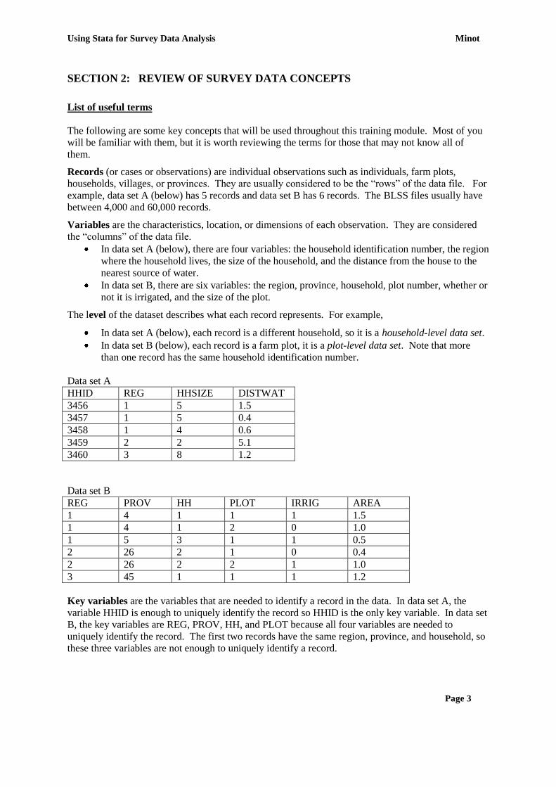
Records (or cases or observations) are individual observations such as individuals, farm plots,
households, villages, or provinces. They are usually considered to be the “rows” of the data file. For
example, data set A (below) has 5 records and data set B has 6 records. The BLSS files usually have
between 4,000 and 60,000 records.
Variables are the characteristics, location, or dimensions of each observation. They are considered
the “columns” of the data file.
In data set A (below), there are four variables: the household identification number, the region
where the household lives, the size of the household, and the distance from the house to the
nearest source of water.
In data set B, there are six variables: the region, province, household, plot number, whether or
not it is irrigated, and the size of the plot.
The level of the dataset describes what each record represents. For example,
In data set A (below), each record is a different household, so it is a household-level data set.
In data set B (below), each record is a farm plot, it is a plot-level data set. Note that more
than one record has the same household identification number.
Data set A
HHID REG HHSIZE DISTWAT
3456 1 5 1.5
3457 1 5 0.4
3458 1 4 0.6
3459 2 2 5.1
3460 3 8 1.2
Data set B
REG PROV HH PLOT IRRIG AREA
1 4 1 1 1 1.5
1 4 1 2 0 1.0
1 5 3 1 1 0.5
2 26 2 1 0 0.4
2 26 2 2 1 1.0
3 45 1 1 1 1.2
Key variables are the variables that are needed to identify a record in the data. In data set A, the
variable HHID is enough to uniquely identify the record so HHID is the only key variable. In data set
B, the key variables are REG, PROV, HH, and PLOT because all four variables are needed to
uniquely identify the record. The first two records have the same region, province, and household, so
these three variables are not enough to uniquely identify a record.

Minot Using Stata for Survey Analysis
Page 4
Discrete variables (or categorical variables) are variables that have only a limited number of different
values. Examples include region, sex, type of roof, and occupation. Yes/no variables such as whether
a household has electricity are also discrete variables.
Binary variables (or dummy variables) are a type of discrete variable that only takes two values.
They may represent yes/no, male/female, have/don‟t have, or other variables with only two values.
Continuous variables are variables whose values are not limited. Examples include per capita
expenditure, farm size, number of trees, rice consumption, coffee production, and distance to the road.
Unlike discrete variables, continuous variables are usually expressed in some units such as dollars,
kilometers, hectares, or kilograms. Also, continuous variables may take fractional values (4.56).
Variable labels are longer names associated with each variable to explain them in tables and graphs.
For example, the variable DISTWAT might have a label “Distance to water (km)” and the variable
REGION could have a label “Region of Bhutan”. Whenever possible, variable labels should include
the unit (e.g. km).
Value labels are longer names attached to each value of a categorical variable. For example, if the
variable REG has four values, each value is associated with a name. The value lables for REG=1
could be “Northern Region”, REG=2 could be the “Central Region”, and so on.
Structure of BLSS data files
The 2003 Bhutan Living Standards Survey was carried out from 5 April to 30 June 2003. The BLSS
had two types of questionnaires: a household questionnaire and a community-price questionnaire.
The household questionnaire consists of a number of sections, as described below:
Household identification
Household roster
Block 1: Housing
Block 2.1: Demographics
Block 2.2: Education
Block 2.3: Health
Block 2.4: Employment
Block 2.5: Information on parents
Block 3: Asset ownership
Block 4: Access and distance to services
Block 5: Remittances sent
Block 6: Priorities, opinions, and miscellaneous
Block 7: Main sources of income
Block 8: Food consumption
Block 9: Non-food consumption
Block 10: Home produced non-food items
Each file contains the data for one or more Blocks. Within each file, the many of the variables are
named according to the block and question question number. For example, in the variable b23_q8
refers to Block 2.3, question 8, a question about whether the individual has ever attended school.
Sometimes, the question has two related responses, such as the quantity and unit. An extra letter is
added to the variable name to distinguish the variables. For example, b24_q47m is the number of
hours devoted to working on the main occuption and b24_q47s is the number of hours in the
secondary occupation.

Using Stata for Survey Data Analysis Minot
Page 5
SECTION 3: INTRODUCTION TO STATA
When you open Stata, you will see a screen similar to the following:
Example 1: View of Stata when first opened
The top row is a menu bar with commands. Below the menu bar is a tool bar with buttons. And there
are four windows labeled Review, Variable, Results, and Command. Each is described briefly below,
along with other windows that can be opened.
Menu bar
The menu bar has lists of commands that can be opened by clicking on a word. There are too many
sub-commands to list here, but below is a list of the main operations that can be done with each
command. If you use Stata a lot, you probably will not use the menu bar often because the most
common tasks can be done with the buttons on the tool bar and key-strokes.
Minot Using Stata for Survey Analysis
Page 6
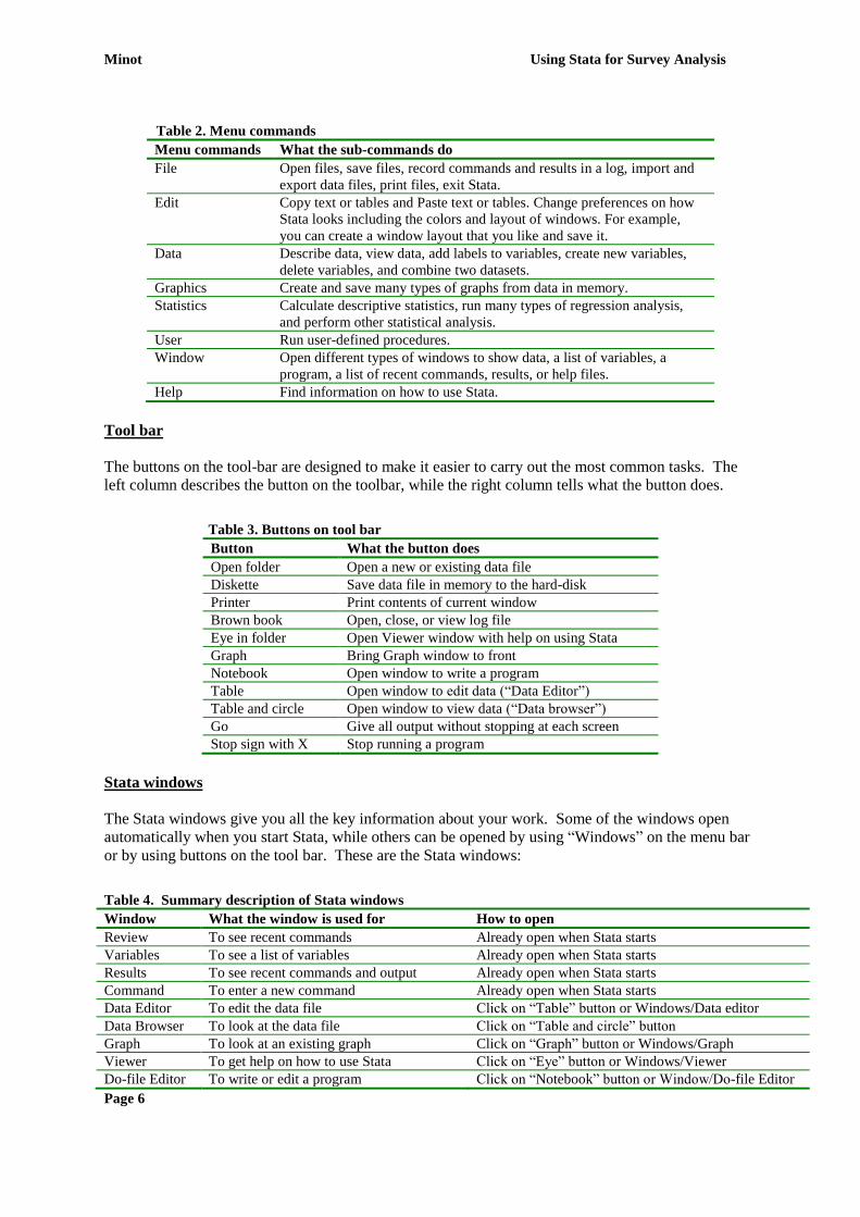
Table 2. Menu commands
Menu commands What the sub-commands do
File Open files, save files, record commands and results in a log, import and
export data files, print files, exit Stata.
Edit Copy text or tables and Paste text or tables. Change preferences on how
Stata looks including the colors and layout of windows. For example,
you can create a window layout that you like and save it.
Data Describe data, view data, add labels to variables, create new variables,
delete variables, and combine two datasets.
Graphics Create and save many types of graphs from data in memory.
Statistics Calculate descriptive statistics, run many types of regression analysis,
and perform other statistical analysis.
User Run user-defined procedures.
Window Open different types of windows to show data, a list of variables, a
program, a list of recent commands, results, or help files.
Help Find information on how to use Stata.
Tool bar
The buttons on the tool-bar are designed to make it easier to carry out the most common tasks. The
left column describes the button on the toolbar, while the right column tells what the button does.
Table 3. Buttons on tool bar
Button What the button does
Open folder Open a new or existing data file
Diskette Save data file in memory to the hard-disk
Printer Print contents of current window
Brown book Open, close, or view log file
Eye in folder Open Viewer window with help on using Stata
Graph Bring Graph window to front
Notebook Open window to write a program
Table Open window to edit data (“Data Editor”)
Table and circle Open window to view data (“Data browser”)
Go Give all output without stopping at each screen
Stop sign with X Stop running a program
Stata windows
The Stata windows give you all the key information about your work. Some of the windows open
automatically when you start Stata, while others can be opened by using “Windows” on the menu bar
or by using buttons on the tool bar. These are the Stata windows:
Table 4. Summary description of Stata windows
Window What the window is used for How to open
Review To see recent commands Already open when Stata starts
Variables To see a list of variables Already open when Stata starts
Results To see recent commands and output Already open when Stata starts
Command To enter a new command Already open when Stata starts
Data Editor To edit the data file Click on “Table” button or Windows/Data editor
Data Browser To look at the data file Click on “Table and circle” button
Graph To look at an existing graph Click on “Graph” button or Windows/Graph
Viewer To get help on how to use Stata Click on “Eye” button or Windows/Viewer
Do-file Editor To write or edit a program Click on “Notebook” button or Window/Do-file Editor

Using Stata for Survey Data Analysis Minot
Page 7
Each is described in more detail below.
Review window This window (in the upper left corner with a white background) lists all the recent
commands. If you click on one of the commands, it appears in the Command window and can be
executed by pressing the “Enter” key. The slide bar can be used to view earlier commands.
Variables window This window (in the lower left corner with a white background) lists all the
variables that exist in memory. When you open a Stata data file, it lists the variables in the file. If
you create new variables, they will be added to the list of variables. If you delete variables, they will
be removed from the list. You can insert a variable into the Stata Command window by clicking on it
in the Variables window.
Results window This window (on the right with a black backgound) shows all recent commands,
output, and error messages. The text is color-coded as follows:
white Stata commands
green General information and the frame and headings of output tables
blue Commands or error messages that can be clicked on for more information
yellow Numbers in output tables
red Error messages
The slide bar on the right side can be used to look at earlier results that are not on the screen.
However, unlike SPSS, the Stata results window does not keep all output generated. It will keep
about 300-600 lines of the most recent output, deleting earlier output. If you want to store output in a
file, you must use the log command.
Command window This window (at the bottom with a white background) allows you to enter
commands which will be executed as soon as you press the “Enter” key. You can also use recent
commands again by using the PageUp key (to go to the previous command) and PageDown key (to go
to the next command). If you click on a variable in the Variable window, it will appear in the
Command window.
Data Editor window This window shows all the data in memory and allows you to change the data.
We do not recommend using this window because you will have no record of the changes you make
in the data. It is better to correct errors in the data using a Do-file program that can be saved.
Data Browser window This window shows all the data in memory. To open the Data Browser, click
on the “table and circle” button. Unlike SPSS, when the Stata Browser is open, you cannot execute
any commands. In addition, you also cannot change any of the data. You can, however, sort the data
or hide certain variables using buttons at the top of the Data Browser window.
Graph window This window shows the results of recent graphs you have created. It can be opened
by clicking on the second “box” button or clicking on Windows/Graph.
Viewer window This window provides help on Stata commands and rules. To use the Viewer
window, type a command in the space at the top and the Viewer will give you the purpose and rules
for using that command, along with some examples. Any blue text in the Viewer can be clicked on
for more information about that command. You can also get help on a specific command by typing
“help [name of command]” in the Command window. The Viewer window can be opened by clicking
on Windows/Viewer.
Do-file Editor window This window allows you to write, edit, save, and execute a Stata program
(like the Syntax Editor window in SPSS). A Stata program (or Do-file) is simply a set of Stata
commands written by the user. The advantage of using the Do-file Editor rather than the Command
window is that the Do-file allows you to save, revise, and rerun a set of commands. Exploratory
analysis of the data can be done with the menu system or the Command window, but most data
Minot Using Stata for Survey Analysis
Page 8
analysis should be carried out using the Do-file Editor. The Do-File Editor can be opened by clicking
on Windows/Do-file Editor or by clicking on the “Notebook” button.
With so many windows, it is sometimes difficult to fit them all on the screen. You can adjust the size
and position of each window the way you like it and then save the layout by clicking on
Edit/Preferences/Manage Preferences/Save Preferences/New Preference Set. The next time you open
Stata, the windows will be arranged according to your preferred layout.
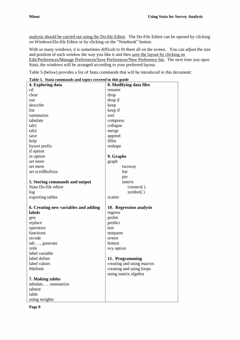
Table 5 (below) provides a list of Stata commands that will be introduced in this document:
Table 5. Stata commands and topics covered in this guide
4. Exploring data
cd
clear
use
describe
list
summarize
tabulate
tab1
tab2
save
help
bysort prefix
if option
in option
set more
set mem
set scrollbufsize
5. Storing commands and output
Stata Do-file editor
log
exporting tables
6. Creating new variables and adding
labels
gen
replace
operators
functions
recode
tab …, generate
xtile
label variable
label define
label values
#delimit
7. Making tables
tabulate … summarize
tabstat
table
using weights
8. Modifying data files
rename
drop
drop if
keep
keep if
sort
compress
collapse
merge
append
fillin
reshape
9. Graphs
graph
twoway
bar
pie
matrix
connect( )
symbol( )
scatter
10. Regression analysis regress
probit
predict
test
testparm
ovtest
hettest
svy option
11. Programming
creating and using macros
creating and using loops
using matrix algebra

Using Stata for Survey Data Analysis Minot
Page 9
SECTION 4: EXPLORING DATA FILES
This section covers commands that are used for preliminary exploration of data in a file. The
following commands and topics are described:
cd
clear
use
describe
list
summarize
tabulate
bysort prefix
if option
in option
save
help
set mem/ more/ scrollbufsize
cd
The cd (change directory) command can be used on its own to identify the directory you are currently
working in. The command, followed by a directory name, changes the directory you work in. Note
that if your directory path contains embedded spaces, you will need to put the path in double quotes.
clear
The clear command deletes all files, variables, and labels from the memory to get ready to use a new
data file. You can clear memory using the clear command or by using the clear subcommand as part
of the use command (see the use command). This command does not delete any data saved to the
hard-drive.
use
This command opens an existing Stata data file. It is equivalent to “get” in SPSS. The syntax is:
use filename [, clear ] opens new file
use [varlist] [if exp] [in range] using filename [, clear ] opens selected parts of file
where filename is the name of a file, varlist is a list of variables, and exp is an expression. The word
in bold are Stata commands, while the others are the names of files and variables and other words
If you do not include an extension, Stata assumes it is .dta.
If you do not include a path, Stata assumes it is in the current folder.
You can use a path name such as: use d:\data\foodexpend
If the path name has spaces, you must use double quotes: use “d:\data\food expenditure”
You can open a selected variables of a file using a variable list.
You can open selected records of a file using if or in.
Here are some examples of the use command:
use household, clear opens the file households.dta
use household 3 if stratum==1 opens data from one stratum (1=urban)
use household in 5/25 opens records 5 through 25 of file
use dzongkha town block in household opens 3 variables from houseold.dta
use d:\data\BLSS\household opens the file tblhousing.dta in the specified
folder
use “d:\data\BLSS\price data” use quotation marks if there are spaces
Minot Using Stata for Survey Analysis
Page 10
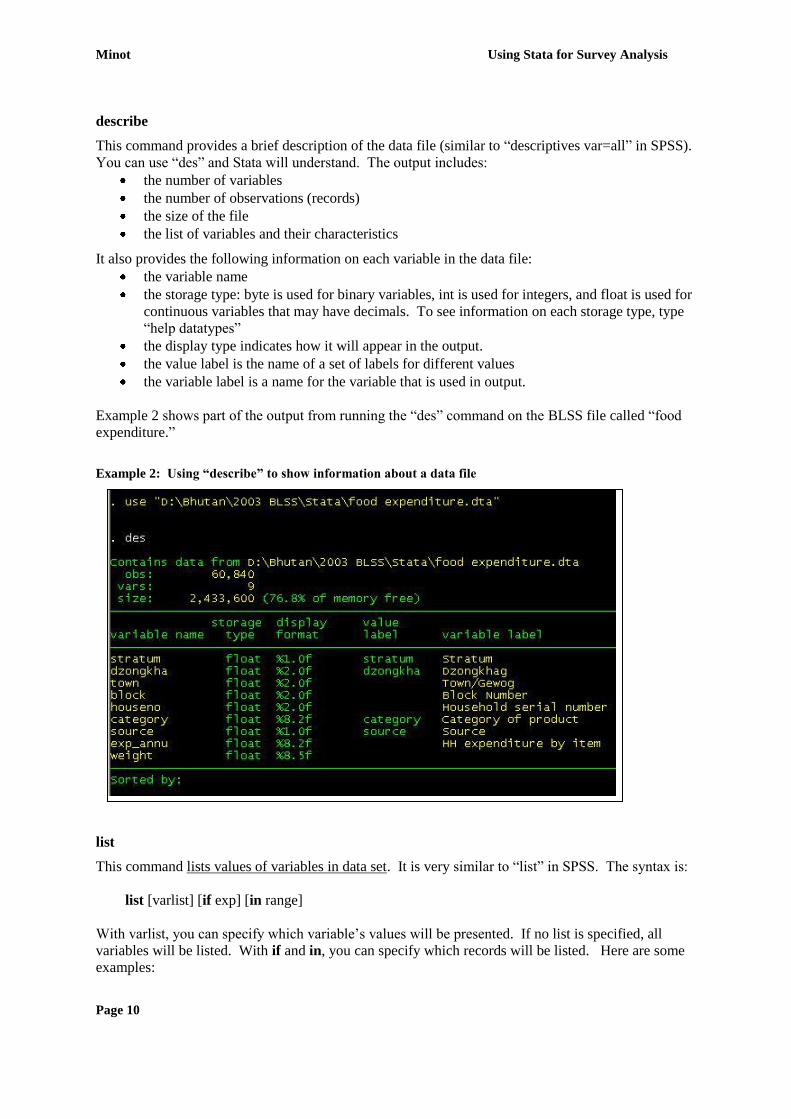
describe
This command provides a brief description of the data file (similar to “descriptives var=all” in SPSS).
You can use “des” and Stata will understand. The output includes:
the number of variables
the number of observations (records)
the size of the file
the list of variables and their characteristics
It also provides the following information on each variable in the data file:
the variable name
the storage type: byte is used for binary variables, int is used for integers, and float is used for
continuous variables that may have decimals. To see information on each storage type, type
“help datatypes”
the display type indicates how it will appear in the output.
the value label is the name of a set of labels for different values
the variable label is a name for the variable that is used in output.
Example 2 shows part of the output from running the “des” command on the BLSS file called “food
expenditure.”
Example 2: Using “describe” to show information about a data file
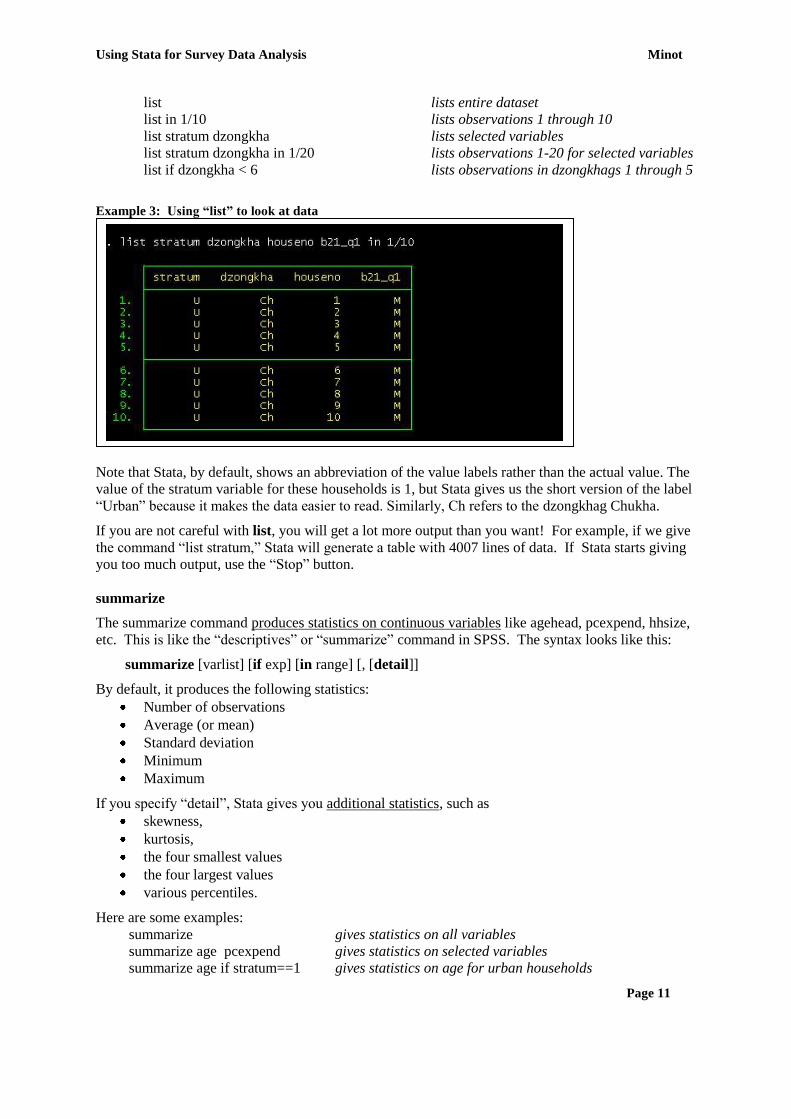
list
This command lists values of variables in data set. It is very similar to “list” in SPSS. The syntax is:
list [varlist] [if exp] [in range]
With varlist, you can specify which variable‟s values will be presented. If no list is specified, all
variables will be listed. With if and in, you can specify which records will be listed. Here are some
examples:
Using Stata for Survey Data Analysis Minot
Page 11
list lists entire dataset
list in 1/10 lists observations 1 through 10
list stratum dzongkha lists selected variables
list stratum dzongkha in 1/20 lists observations 1-20 for selected variables
list if dzongkha < 6 lists observations in dzongkhags 1 through 5
Example 3: Using “list” to look at data
Note that Stata, by default, shows an abbreviation of the value labels rather than the actual value. The
value of the stratum variable for these households is 1, but Stata gives us the short version of the label
“Urban” because it makes the data easier to read. Similarly, Ch refers to the dzongkhag Chukha.
If you are not careful with list, you will get a lot more output than you want! For example, if we give
the command “list stratum,” Stata will generate a table with 4007 lines of data. If Stata starts giving
you too much output, use the “Stop” button.
summarize
The summarize command produces statistics on continuous variables like agehead, pcexpend, hhsize,
etc. This is like the “descriptives” or “summarize” command in SPSS. The syntax looks like this:
summarize [varlist] [if exp] [in range] [, [detail]]
By default, it produces the following statistics:
Number of observations
Average (or mean)
Standard deviation
Minimum
Maximum
If you specify “detail”, Stata gives you additional statistics, such as
skewness,
kurtosis,
the four smallest values
the four largest values
various percentiles.
Here are some examples:
summarize gives statistics on all variables
summarize age pcexpend gives statistics on selected variables
summarize age if stratum==1 gives statistics on age for urban households

Minot Using Stata for Survey Analysis
Page 12
Example 4. Using “summarize” to study continuous variables
The first example gives the statistics for the whole sample of 4007 households, while the second gives
the statistics only for households in stratum 1, urban areas. The variable b21_q3ag refers to the age of
the head of household, so the tables above indicate that urban households are youger, richers, and
smaller than the average household in Bhutan.
tabulate, tab1, tab2
These are three related commands that produce frequency tables for discrete variables. They can
produce one-way frequency tables (tables with the frequency of one variable) or two-way frequency
tables (tables with a row variable and a column variables. These commands are similar to the
“frequency” and “crostab” commands in SPSS. How do the three commands differ?
tabulate or tab produce a frequency table for one or two variables
tab1 produces a one-way frequency table for each variable in the variable list
tab2 produces all possible two-variable tables from the list of variables
You can use several options with these commands:
all gives all the tests of association for two-way tables
cell gives the overall percentage for two-way tables
col gives column percentages for two-way tables
row gives row percentages for two-way tables
nofreq suppresses printing the frequencies
nol suppresses the use of value labels, showing the numeric values instead
chi2 provides the chi squared test for two-way tables
There are many other options, including other statistical tests. For more information, type “help
tabulate”.
Some examples of the tabulate commands are:
tabulate dzongkha produces table of frequency by dzonghka
tabulate dzongkha b21_q1 produces a cross-tab by dzongkhag and sex of head
tabulate dzongkha b21_q1, row produces the same cross-tab with row percentages
tab1 dzongkha b21_q1 hh_size produces three tables, a frequency table for each variable

Using Stata for Survey Data Analysis Minot
Page 13
tab2 dzongkha b21_q1 hh_size produces three tables, a cross-tab of each pair of variables
Each type of tabulate command gives somewhat different output:
In one-way tables, Stata gives the count, the percentage, and the cumulative percentage (see
first example in box).
In two-way tables, Stata gives the count only, unless you ask for other statistics (see second
example in box)
col, row, and cell request Stata to include percentages in two-way tables
Example 5 shows the output of three types of tab commands: a one-way frequency table, a two-way
frequency table, and a two-way frequency table with row and column percentages. Although the
stratum variable has the values 1 and 2, the table shows the labels associated with each value,
“Urban” and “Rural”, respectively. Section 6 describes how to create and work with labels.
Example 5. Using “tabulate” on categorical variables
Minot Using Stata for Survey Analysis
Page 14
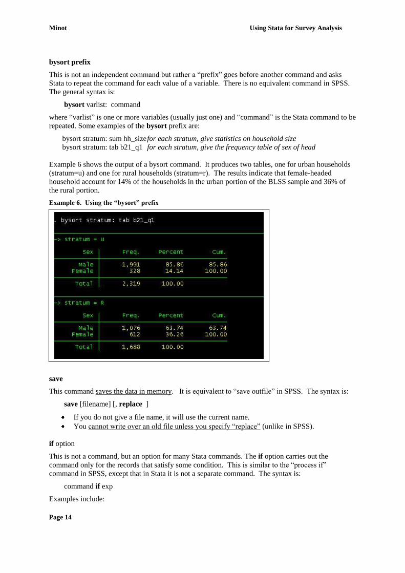
bysort prefix
This is not an independent command but rather a “prefix” goes before another command and asks
Stata to repeat the command for each value of a variable. There is no equivalent command in SPSS.
The general syntax is:
bysort varlist: command
where “varlist” is one or more variables (usually just one) and “command” is the Stata command to be
repeated. Some examples of the bysort prefix are:
bysort stratum: sum hh_size for each stratum, give statistics on household size
bysort stratum: tab b21_q1 for each stratum, give the frequency table of sex of head
Example 6 shows the output of a bysort command. It produces two tables, one for urban households
(stratum=u) and one for rural households (stratum=r). The results indicate that female-headed
household account for 14% of the households in the urban portion of the BLSS sample and 36% of
the rural portion.
Example 6. Using the “bysort” prefix
save
This command saves the data in memory. It is equivalent to “save outfile” in SPSS. The syntax is:
save [filename] [, replace ]
If you do not give a file name, it will use the current name.
You cannot write over an old file unless you specify “replace” (unlike in SPSS).
if option
This is not a command, but an option for many Stata commands. The if option carries out the
command only for the records that satisfy some condition. This is similar to the “process if”
command in SPSS, except that in Stata it is not a separate command. The syntax is:
command if exp
Examples include:

Using Stata for Survey Data Analysis Minot
Page 15
list hh_size if dzongkha<4 lists all household sizes for dzongkhags 1, 2, and 3
tab hh_size if stratum==2 gives number of rural households of each size
sum b21_q3ag if b21_q1==2 gives statistics on age for female-headed households
Note that “if” statements always use two equal symbols (==), not just one. Also note that | indicates
“or” while & indicates “and”.
in
This is not a command, but an option for many Stata commands. The in option carries out a command
only for records selected by the case number. The syntax is:
command in exp
For example:
list hh_size in 10 give the value of hh_size in observation number 10
summarize in 10/20 give mean, minimum, and maximum of all variables for observations
10-20 .
help
The help command gives you information about any Stata command or topic
help command
For example,
help tabulate gives a description of the tabulate command
help summarize gives a description of the summarize command
set
The set command is used to control the Stata operating environment. There are dozens of set
commands, but many of them are rarely used. Some of the more common ones are:
set mem XXm sets memory for Stata at XX megabytes. If you get the error message “No room to
add more observations”, this means the data file is too big for the memory allocated to Stata. This
command increases the memory allocated to Stata. You cannot set XX greater than the total RAM
memory in the computer – physical and virtual memory.
set more off/on is used to turn on and off the continuous scrolling of output. Use “set more off” if
you are not interested in the intermediate output, only the final result. Use “set more on” if you need
to be able to read the early output. Remember that the Results Window only stores the most recent
300-600 lines of output. Unlike SPSS, Stata does not automatically store all of your output.
set scrollbufsize XX is used to change the amount of output that Stata will store in the Results
window. XX is expressed in bytes. The default is 32,000 (32k) and the maximum is 500,000 (500k).
Type “help set” for a list of other settings in Stata.
Exercises for exploring the BLSS
Here are some questions that you can answer using the BLSS files provided on your computer and the
commands described in this section. The file households.dta contains summary variables calculated
from various other data files. It is at the household level. Open the file by entering “use household”
in the Command window and pressing “Enter.”
1. How many variables and how many records are in the file households.dta? (Hint: use
“describe”)
2. What percentage of households have female heads? (Hint: tab b21_q1)

Minot Using Stata for Survey Analysis
Page 16
3. Is there a statistically significant difference between the percentage of female-headed
households in urban and rural areas? (Hint: use tab command with the chi2 option)
4. What percentage of urban households are female headed household? (Hint: use “if
stratum==1” option)
5. What percentage of female households are in urban areas?
6. How does the percentage of female headed household vary across dzongkhags?
7. What is the average size of a household?
8. What is the average size of an urban household in Paro? (Hint: Paro is dzongkhag #3)
Note: The purpose of these exercises is to practice the Stata commands. To get the correct answers,
we would have to use the sample weights which are described in Section 7. The weights compensate
for the fact that some types of households are over-represented in the BLSS sample and others are
under-represented.

Using Stata for Survey Data Analysis Minot
Page 17
SECTION 5: STORING COMMANDS AND OUTPUT
In this section, we discuss how to store commands and output for later use. First, we describe how to
store commands a program (Stata calls it a Do-file) , how to edit the program, and how to run it.
Second, we present different ways of saving and using the output generated by Stata. The following
topics are covered:
using the Do-file Editor
log using
log off
log on
log close
set logtype
moving tables from Stata to Word and Excel
Using the Do-file Editor
As mentioned in Section 3, a Do-file is a file that stores a Stata program (a set of commands) so that
you can edit it and run it later. The Do-file Editor is like a simplified word processor for writing Stata
programs. Why use the Do-file Editor rather than the Command window or the menu system?
It makes it easier to check and fix errors,
it allows you to run the commands later,
it lets you show others how you got your result, and
it allows you to collaborate with others on the analysis.
In general, any time you are running more than 5-10 commands to get a result, it is easier and safer to
use a Do-file to store the commands.
To open the Do-file Editor, you can click on Windows/Do-file Editor or click on the “Notebook”
button on the Tool Bar. Within the Do-file Editor, there is a menu bar and tool bar buttons to carry
out a variety of editing functions. The menu is a simplified version of menus in MS Word and other
word processors. Here are some of the more important commands in the menu bar of the Do-file
Editor:
File/New to open a new, blank Do-file
File/Open to open an existing Do-file
File/Save to save the current Do-file
File/Save as to saving the current Do-file under a new name
File/Insert file to insert another file into the current one
File/Print to print the Do-file
File/Close to close the Do-file
Edit/Undo to undo the last command
Edit/Cut to delete or move the marked text in the Do-file
Edit/Copy to copy the marked text in the Do-file
Edit/Paste to insert the copied or cut text into the Do-file
Search/Find to find a word or phrase in the Do-text
Search/Replace to find and replace a word or phrase in the Do-file
Tools/Do to execute all the commands or the marked commands in the Do-file
Tools/Run to execute all the commands or the marked commands in the Do-file without
showing any output in the Stata Results window
The tool bar buttons can be used to carry out some of these tasks more quickly. For example, there
are buttons for File/New, File/Open, File/Print, Search/Find, Edit/Cut, Edit/Copy, Edit/Paste,

Minot Using Stata for Survey Analysis
Page 18
Edit/Undo, Do, and Run. Probably the button you will use most is the third-to-last one that shows a
page with text on it. This is the “Do” button for executing the program or the marked part of the
program.
Finally, many of the keyboard commands in MS Word work in the Do-file Editor. For example,
control-Z to undo, control-C to copy, control-V to paste, control-X to delete, and control-F to find.
To run the commands in a Do-file, you can click on the Do button (the third-to-last one) or click on
Tools/Do. If you want to run one or just a few commands rather than the whole file, mark the
commands and click on the Do button. You do not have to mark the whole command, but at least one
character in the command must be marked in order for the command to be executed (unlike SPSS, it is
not enough to have the cursor on a command).
Although layout is a matter of personal preference, it may be useful to have the Results window and
the other windows on one side of the screen and the Do-file Editor window on the other. This makes
it easy to switch back and forth. When you arrange the windows the way you like, you can save the
layout by clicking Prefs/Manage Preferences/Save Preferences. Each time you open Stata, it will use
your chosen layout.
Saving the output
As mentioned in Section 3, the Stata Results window does not automatically keep all the output you
generate. It only stores about 300-600 lines, and when it is full, it begins to delete the old results as
you add new results. You can increase the amount of memory allocated to the Stata Results window
(see “set scrollbufsize” in Section 3), but even this will probably not be enough for a long session with
Stata. Thus, we need to use log to save the output.
There are several different ways to control the log operations.
You can use the “Brown book” button on the tool bar.
You can click on File/Log to begin or close a log file (Suspend and Resume are to temporarily
turn off and on the log).
You can use “log” commands in the Command window
You can use “log” commands in a Do-file.
In this section, we describe the commands, which can be used in the Stata Command window or in a
do-file (program).
log using
This command creates a file with a copy of all the commands and output from Stata. The first time
you open a log, you must give a name to the new file to be created. The syntax is:
log using filename [, append replace [ text | smcl ] ]
where filename is that name you give the new file. The options are:
append adds the output to an existing file
replace replaces an existing file with the output
text tells Stata to create the log file in text (ASCII) format
smcl tells Stata to create the log file in SMCL format
Here are some examples:
log using temp22 saves output to a file called temp22
log using temp20, replace saves output to an existing file, replacing content
log using temp20, append saves output to an existing file, adding to contents
log using “d:/BLSS/temp24”, text saves output in specified file in specified folder in text format
Several points should be remembered in using this command:
Using Stata for Survey Data Analysis Minot
Page 19
if you use an existing file name but do not say “replace” or “append”, Stata will give an error
message that the file already exists
log files in text format can be opened with Wordpad, Notepad, the DOS editor, or any word
processor., but the file will not have any formatting (e.g. no colors, bold, italics, or
underlines)
smcl files have formatting (bold, colors, etc) but can only be opened with Stata
smcl format is the default
log off
This command temporarily turns off the logging of output, so that any subsequent output is not copied
to the log file. This is useful if you want to save some of the output but not all. “Log off” only works
after a “log using command.”
log on
This command is used to restart the logging, copying any new output to the log file that was already
defined. “Log on” only works after a “log using” and a “log off” command.
log close
This command is used to turn off the logging and save the file. How are “log off” and “log close”
different? “Log off” allows you to turn it back on easily with “log on,” continuing to use the same
log file. After a “log close” however, the only way to start logging again is with “log using.”
set logtype text
This command tells Stata to always save the log files in text (ASCII) format. It is the same as adding
the “text” subcommand to every “log using” command, but it is easier. If you prefer text format files
(as we do), this is the best way to make sure all the log files are in this format.
set logtype smcl
This command tells Stata to always save log files in SMCL format. It is the same as adding the
“smcl” subcommand to every “log using” command.
Example 7 shows how the log command can be used. First, the log is opened using the filename
“temp1.” Since no folder was specified, it saved the file to the current default folder. The results
from “tab urban” are saved in the log file. Then the log is turned off, so the results of “sum hhsize” is
not logged. Third, the log is turned on so the results from “sum agehead” are logged. Finally, the log
is closed.
Example 7 shows the operation of the log command. In order to save the table we are going to create,
we enter the command “log using hhtable, text”. By using the text option, we are telling Stata to save
the log file in text (ASCII) format. What ever is produced by Stata after this point will be recorded in
the log file. Later, we use the “log off” command to stop recording.

Minot Using Stata for Survey Analysis
Page 20
Example 7: Using “log” to save output
Using Stata output
To look at a log file, the easiest way is to click on File/Log/View. However, there are numerous other
ways to do it, including clicking on the Eye buttom, opening it from the Do-File Editor, and opening it
from WordPad.
To print output from the Results window, you can click File/Print Results.
To print output from a log file, you open the log file with Viewer (File/Log/View) and then click on
File/Print/Viewer.
Unfortunately, it is not easy to copy Stata output to other software such as word processors and
spreadsheets. It is best to copy tables from a log file or from the Results window using Edit/Copy
Table.
To move tables from a log file to an Excel table,
1) Open the log file by clicking on File/Log/View
2) Mark the table by dragging the cursor across it

Using Stata for Survey Data Analysis Minot
Page 21
3) Copy the table with Edit/Copy Table or Control-Shift C
4) Paste the table into Excel
To move tables from a log file to a Word table,
1) Open the log file by clicking on File/Log/View
2) Mark the table by dragging the cursor across it
3) Copy the table with Edit/Copy Table or Control-Shift C
4) Paste the table into Word with Control-V
5) Mark the table and then click Table/Insert/Table
To move tables from the Results window to Word or Excel, follow the above procedures starting with
step #2.
However, one problem with these procedures is that there has to be a clear division between columns.
If there is a heading that overlaps two columns, the two columns will be merged. To avoid this, you
can exclude the heading when you copy the table.
Exercises for saving commands and output
1) Open a do-file (program) to store commands and write a program that 1) opens the
households.dta data file and 2) produces a table showing the percentage of female-headed
households in urban and rural areas (hint: use the tab command). Run the program to make
sure it works. Save the program as “table1” and then exit.
2) Open the program “table1” and add a command to create a second table showing the number
of sample households in each dzongkhag. Run, save, and close.
3) Open the program “table1” and a log commands to save the output to a file called
“table1_results”. Be sure to include both a “log using..” command and a “log off” command.
4) Copy one of the tables into Excel using the Edit/Copy table menu command.
5) Copy the table into a Word file.

Minot Using Stata for Survey Analysis
Page 22
SECTION 6: CREATING NEW VARIABLES AND ADDING LABELS
In the previous sections, we described how to explore the data using existing variables. In this
section, we discuss how to create new variables and how to label them. When new variables are
created, they are in memory and they will appear in the Data Browser, but they will not be saved on
the hard-disk unless you use the save command.
In this section, we will cover the following commands and topics:
generate
replace
tab …, generate
using operators
using functions
recode
xtile
label variable
label define
label values
#delimit
generate
This command is used to create a new variable. It is similar to “compute” in SPSS. The syntax is:
generate newvar = expression [if exp]
where “expression” is a mathematical statement like “price*quant” or “quant_kg/1000”. Several
points about this command: :
Unlike “compute” in SPSS, you cannot use “generate” to change the definition of an existing
variable. If you want to change an existing variable, you need to use “replace,”
You can use “gen” as an abbreviation for “generate”
If the expression is an equality or inequality, such as (age>15), then the new variable will take
the values 0 if the expression is false and 1 if it is true
If you use “if”, the new variable will have missing values when the “if” statement is false
For example,
generate agehead2 = agehead*agehead create agehead squared variable
. gen yield = quant/area if area>0 create new yield variable if area is positive
gen price = value/quant if quant>0 create new price variable if quant is positive
gen highprice = (price>1000) creates a dummy variable equal to 1 if the price is
greater than 1000 and 0 otherwise
replace
This command is used to change the definition of an existing variable. The syntax is the same:
replace oldvar = expression [if exp] [in exp]
Some points to remember:
Replace cannot be used to create a new variable. Stata will give an error message if the
variable does not exist.
There is no abbreviation for “replace.” Stata wants to make sure you really want to change it.

Using Stata for Survey Data Analysis Minot
Page 23
If you use the “if” option, then the old values will be retained when the “if” statement is false
You can use the period (.) to represent missing values
For example,
replace price = avgprice if price > 100000 replaces high values with an average price
replace pcexpend =. if pcexpend<=0 replace negative pcexpend with missing value
replace agehead = 25 in 1007 replace age=25 in observation #1007
Example 8 shows the use of the gen and replace commands to create a new variable called region.
The new variables has three values: 1 for west, 2 for center, and 3 for east.
Example 8: Using “generate” and “replace” to create new variables
tabulate … generate
This command is useful for creating a set of dummy variables (variables with a value of 0 or 1)
depending on the value of an existing categorical variable. The syntax is:
tabulate oldvariable, generate(newvariable)
It is easier to explain with an example. Suppose we want to create three dummy variables that
indicate whether a household is in the west, center, or east of Bhutan. We can create three dummy
variables from the variable “region” as follows:
tab region, gen(reg)
This creates three new variables, defined as follows:
reg1=1 if region=1 and 0 otherwise
reg2=1 if region=2 and 0 otherwise
reg3=1 if region=3 and 0 otherwise
In the example below, notice that there are 1746 households in region 1 (west) and the same number
of households for which reg1 = 1.

Minot Using Stata for Survey Analysis
Page 24
Example 9: Using “tab…gen” to create dummy variables
egen
This is an extended version of “generate” to create a new variable by aggregating the existing data. It
is a powerful and useful command that does not exist in SPSS. To do the same thing in SPSS, you
would need to create a new file with “aggregate” and merge it with the original file using “match
files.” The syntax is:
egen newvar = fcn(argument) [if exp] [in range] , by(var)
where newvar is the new variable to be created
fcn is one of numerous functions such as:
count( )
max( )
min( )
mean( )
median( )
rank( )
sd( )
sum( )
argument is normally just a variable
var in the by() subcommand must be a categorical variable
Suppose you want to estimate the demand for rice using the BLSS data. You calculate a price
variable using the data, but some households do not buy rice. You can calculate dzongkhag-level
average price and replace missing values with that average price as follows:
egen avgprice = mean(price), by(province)
replace price=avgprice if price==.
Here are some other examples:
egen avg = mean(yield) creates variable of average yield over entire
sample
egen avg2 = median(pcexpend), by(sexhead) creates variable of median pcexpend for
each sex
egen regprod = sum(prod), by(reg4) creates variable of total production for each
region

Using Stata for Survey Data Analysis Minot
Page 25
In Example 10, we want to know which households have per capita expenditure (pc_t_mo) above the
dzongkhag average. First, we calculate the average expenditure for each villaged with the “egen”
command. Then we create a dummy variable based on the expression (pc_t_mo > avgexp). The list
output shows how the dzongkhag average is repeated for every household and confirms that the
dummy variable is correctly calculated.
Example 10: Using “egen” to calculate averages
Using operators
Operators are symbols used in equations. Most of the operators are obvious (e.g. + and -), but some
are not. Table 6 lists the most commonly used operators. They are similar to the operators in
SPSS, except that in Stata you cannot use words like “or”, “and”, “eq”, or “gt”.
Table 6. Key operators for writing equations in Stata
Operator Meaning Example
+ addition gen income = agincome + nonagincome
- subtraction gen netrevenue = revenue – cost
* multiplication gen value = price * quantity
/ division gen exppc = expenditure/hhsize
^ power gen agesquared = age^2
> greater than gen aboveavg = 1 if income > avgincome
< less than gen belowavg = 1 if income < avgincome
>= more than or equal gen child = 1 if age <=10
<= less than or equal gen adult = 1 if age >= 18
= equal (to set value) gen expend = foodexp + nonfoodexp
== equal (in “if” condition) gen femhead = 1 if sexhead==2
~= not equal gen error = 1 if value1 ~= value2
!= not equal gen error = 1 if value1 != value2
| or gen age=. if age==999 | age=9999
& and gen sexhead = 1 if sex==1 & relation==1
The most difficult rule to remember is when to use = and when to use ==.
Use a single equal symbol (=) when defining a variable.
Use a double equal symbol (==) when you are testing an equality, such as in an “if” statement
and when creating a dummy variable.
Here is a short-cut for creating dummy variables. Suppose you want you create a dummy variable
indicating households in Paro. One way is to write:
generate Paro = 0
Minot Using Stata for Survey Analysis
Page 26
replace Paro = 1 if dzongkha==3
Or you can get exactly the same result with just one command:
generate Paro = (dzongkha==3)
If the expression in parentheses is true, the value is set to 1. If it is false, the value is 0.
The “or” and “and” operators are useful if you want to impose more than one condition. For example,
suppose you want to create a dummy variable for female household heads in Paro. In other words, a
household must be both in the dzongkhag of Paro and be female headed to be selected.
gen Paro_fem = 0
replace Paro_fem = 1 if dzongkha==3 & b21_q1==2
or an easier way to do this would be:
gen Paro_fem = (dzongkha==3 & b21_q1 ==2)
Or suppose you wanted to create a dummy variable for households in the west and central regions.
This means a household can be in the west or it can be in the central Region to be selected. This
variable can be created with:
gen west_cent = 0
replace west_cent = 1 if region==1 | region==2
or by one command:
gen west_cent = (region==1 | region==2)
You can also combine conditions using parentheses. Suppose you wanted a dummy variable that
indicates if a household in one of these regions is headed by a woman. The command would be:
gen west_cent_FP = ((region==1 | region==2) & b21_q1==2)
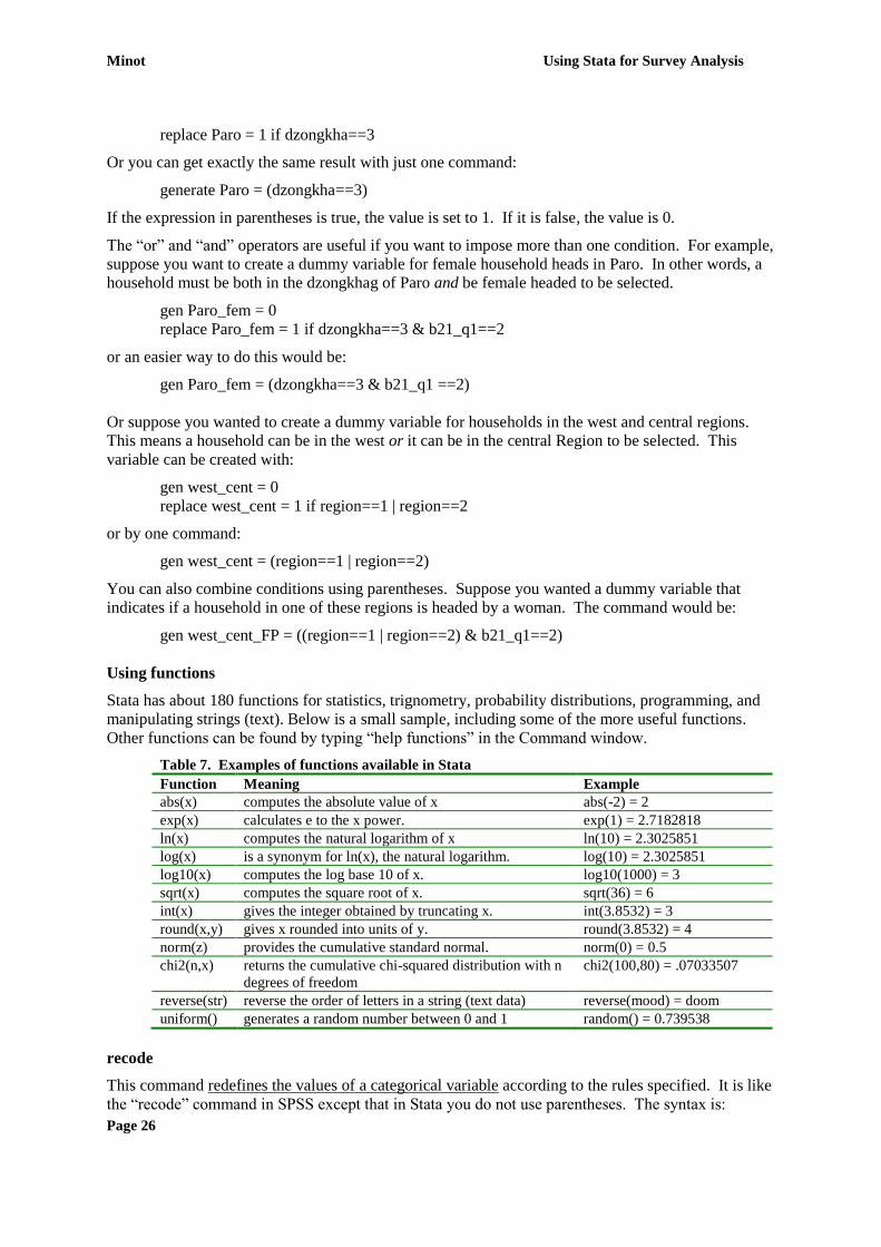
Using functions
Stata has about 180 functions for statistics, trignometry, probability distributions, programming, and
manipulating strings (text). Below is a small sample, including some of the more useful functions.
Other functions can be found by typing “help functions” in the Command window.
Table 7. Examples of functions available in Stata
Function Meaning Example
abs(x) computes the absolute value of x abs(-2) = 2
exp(x) calculates e to the x power. exp(1) = 2.7182818
ln(x) computes the natural logarithm of x ln(10) = 2.3025851
log(x) is a synonym for ln(x), the natural logarithm. log(10) = 2.3025851
log10(x) computes the log base 10 of x. log10(1000) = 3
sqrt(x) computes the square root of x. sqrt(36) = 6
int(x) gives the integer obtained by truncating x. int(3.8532) = 3
round(x,y) gives x rounded into units of y. round(3.8532) = 4
norm(z) provides the cumulative standard normal. norm(0) = 0.5
chi2(n,x) returns the cumulative chi-squared distribution with n
degrees of freedom
chi2(100,80) = .07033507
reverse(str) reverse the order of letters in a string (text data) reverse(mood) = doom
uniform() generates a random number between 0 and 1 random() = 0.739538
recode
This command redefines the values of a categorical variable according to the rules specified. It is like
the “recode” command in SPSS except that in Stata you do not use parentheses. The syntax is:

Using Stata for Survey Data Analysis Minot
Page 27
recode varname oldvalue=newvalue oldvalue=newvalue … [if exp] [in range]
Here are some examples:
recode x 1=2 changes all values of x=1 to x= 2
recode x 1=2 3=4 in the variable x, changes 1 to 2 and 3 to 4
recode x 1=2 2=1 in the variable x, exchanges the values 1 and 2
recode x 1=2 *=3 in the variable x, changes 1to 2 and all other values to 3
recode x 1/5=2 in the variable x, changes 1 through 5 to 2
recode x 1 3 4 5 = 6 in the variable x, changes 1, 3, 4 and 5 to 6
recode x .=9 in the variable x, changes missing to 9
recode x 9=. in the variable x, changes 9 to missing
Notice that you can use some special symbols in the recode command:
* means all other values
. means missing values
x/y means all values from x to y
x y means values x and y
In Example 11, we create a new variable called maritalstat that indicates whether a head of household
is 1) married or separated, 2) never married, or 3) divorced or widowed. It is based on the variable
b21_q4 in the households.dta data file.
Example 11. Using “recode “to define a new variable
xtile
This command creates a new variable that indicates which category a record falls into, when the
sample is sorted by an existing variable and divided into n groups of equal size. It is probably easier
to explain with examples. xtile can be used to create a variable that indicates which pcexpend quintile
a household belongs to, which decile in terms of farm size, or which tercile in terms of coffee
production. The syntax is:
xtile newvar = variable [if exp] [in range] , nq(#)

Minot Using Stata for Survey Analysis
Page 28
where
newvar is the new categorical variable created
variable is the existing variable used to create the quantile (e.g pcexpend, farm size)
# is the number of different categories (eg 5 for quintiles, 3 for terciles)
For example,
pctile incquint = pcexpend, nq(5)
pctile farmdec = farmsize, nq(10)
pctile coffeeter = coffarea, nq(3)
In the example below, we create a variable indicating the tercile of per capita expenditure, using the
variable pc_t_mo in the households.dta data file.
Example 12. Using “xtile” to create categories
label variable
This command is used to attach labels to variables in order to make the output easier to understand.
For example, we know that maritalstat indicates the marital status of the head of household and that
pcetercile means tercile of per capita expenditure. But other people using our tables may not know
this. So we may want to label the variables as follows:
label variable region “Region of country”
label variable pcetercile “Tercile of p.c. expenditure”
You can use the abbreviation “lab var”
If there are spaces in the label, you must use double quotation marks.
If there are no spaces, quotation marks are optional.
This command is like “variable label” in SPSS except that you can only label one variable per
command and Stata uses double quotation marks, not single
The limit is 80 characters for a label, but any labels over 30 characters will probably not look
good in a table.
label define
This command gives a name to a set of value labels. For example, instead of numbering the regions,
we can assign a label to each region. Instead of numbering the different sources of water, we can give
them labels. The syntax is:
label define lblname # "label" # "label" # “label” [, add modify]
Using Stata for Survey Data Analysis Minot
Page 29
where
lblname is the name given to the set of value labels
# are the value numbers
“label” are the value labels
add means that you want to add these value labels to the existing set
modify means that you want to change these values in the existing set
Note that:
You can use the abbreviation “lab def”
The double quotation marks are only necessary if there are spaces in the labels
Stata will not let you define an existing label unless you say “modify” or “add”
This command is similar to “value label” in SPSS except that in Stata you give the labels a
name and later attach it to the variable, while in SPSS you attach it to the variable in the same
command.
label values
This command attaches named set of value labels to a categorical variable. The syntax is:
label values varname lblname
where
varname is the categorical variable which will get the labels
lblname is a set of labels that have already been defined by label define
Here are some examples of labeling values in Stata.
label variable yield "Yield (tons/hectare)" gives label to variable yield
label define yesno 0 no 1 yes defines set of labels called yesno
label values electricity yesno attaches labels to the variable “electricity”
label define yesno 3 "perhaps", add adds new value label to existing set
label define yesno 3 "maybe", modify modifies existing value label
label define reglbl 1 West 2 Center 3 East defines regional labels
label values region reglbl attaches regional labels to region
label define reglbl 2 Central, modify modifies regional labels
Some additional commands that may be useful in labeling
label dir to request a list of existing label names
label list to request a list of all the existing value labels
label drop to delete a one or more labels
label save using to save label definitions as a Do-file
label data to give a label to a data file
More information is available by typing “help label” in the Stata Command window.
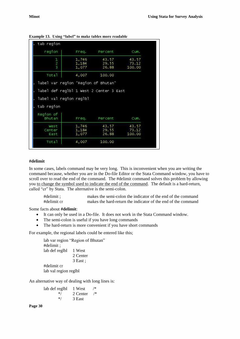
Example 13 shows a frequency table with and without labels. The first table has no labels. Then, the
“label var” command is used to give the “region” a label of “Region of Bhutan”. Next, the “label
define” command creates a label for each region and label values attaches those labels to the “reigon”
variable. The second table has both the variable label (in the upper left corner of the table) and the
labels for each regions.
Minot Using Stata for Survey Analysis
Page 30
Example 13. Using “label” to make tables more readable
#delimit
In some cases, labels command may be very long. This is inconvenient when you are writing the
command because, whether you are in the Do-file Editor or the Stata Command window, you have to
scroll over to read the end of the command. The #delimit command solves this problem by allowing
you to change the symbol used to indicate the end of the command. The default is a hard-return,
called “cr” by Stata. The alternative is the semi-colon.
#delimit ; makes the semi-colon the indicator of the end of the command
#delimit cr makes the hard-return the indicator of the end of the command
Some facts about #delimit:
It can only be used in a Do-file. It does not work in the Stata Command window.
The semi-colon is useful if you have long commands
The hard-return is more convenient if you have short commands
For example, the regional labels could be entered like this;
lab var region “Region of Bhutan”
#delimit ;
lab def reglbl 1 West
2 Center
3 East ;
#delimit cr
lab val region reglbl
An alternative way of dealing with long lines is:
lab def reglbl 1 West /*
*/ 2 Center /*
*/ 3 East

Using Stata for Survey Data Analysis Minot
Page 31
The #delimit command and the /* symbols can be used with any command, but they are often used
with value labels.
Exercises for creating variables and labels
1) Use the file households.dta. Create a variable called “region” using the commands in
Example 8. Now create a variable “region2” which is equal to 1 if the household is in the
west and 2 if the household is in center or east (hint: use the “recode” command). Then do a
frequency table of the new variable.
2) Create value labels for the two values of region2 (hint: use “lable def” and “label val”).
3) Using the same file, create a variable called “hhquint” that indicates the quintile of household
size (hint: use the “xtile” command and hh_size variable). Then do a frequency table on the
new variable.
4) Using the same file, create a dummy variable called “rurfem” that is equal to 1 if the
household is a rural female headed household and 0 otherwise (hint: use the “stratum” and
“b21_q1” variables).
5) Create a new variable “avgexp” which is equal to the regional average of expenditure
(pc_t_mo) (hint: use egen and the region variable created in Exercise #1). Then calculate a
new variable “diff” equal to the difference between the household expenditure and the
regional average expenditure.
6) Create a set of dummy variables called region1, region2, and region3 which are equal to 1 in
regions 1, 2, and 3 respectively and zero elsewhere (hint: use tab…gen).

Minot Using Stata for Survey Analysis
Page 32
SECTION 7: MAKING TABLES TO DESCRIBE DATA
In Section 4, we described some basic commands for exploring data. In this section, we introduce
three powerful and flexible commands for generating results from survey data. We also describe the
use of sampling weights in analyzing survey data. These are the commands and topics covered in
this section:
tabulate … summarize
tabstat
table
using weights
tabulate … summarize
This command creates one- and two-way tables that summarize continuous variables. The command
tabulate by itself gives frequencies and percentages in each cell (cross-tabulations). With the
“summarize” option, we can put means and other statistics of a continuous variable. The syntax is:
tabulate varname1 varname2 [if exp] [in range], summarize(varname3) options
where
varname1 is a categorical row variable
varname2 is a categorical column variable (optional)
varname3 is the continuous variable summarized in each cell
options can be used to tell Stata which statistics you want
Some notes regarding this command:
The default statistics are the mean, the standard deviation, and the frequency.
You can specify which statistics with options “means” “standard” and “freq”
You can use the abbreviation “tab…sum”
This command is similar to the Stata command “bysort var3: sum var3” except that the
“tab…sum” output is more attractive and “tab…sum” allows two categorical variables
This command is also similar to the SPSS command “means var3 by var1”
Some examples:
tab region, sum(pcexpend) gives the mean, std deviation, and frequency of per
capita expenditure for each region
tab stratum, sum(hhsize) mean gives the mean household size for urban and rural
households
tab sexhead stratum, sum(pcexpend) gives the mean, std deviation, and frequency of per
capita expenditure in each cell of a 2x2 table of
male/female headed and urban/rural households
In Example 14, we give the output for three “tab…sum” commands. First, “xtile” is used to create a
variable “pcetercile” which indicates whether a household is in the top, middle, or bottom third in
terms of per capita expenditure.
The first table is a one-way table (just one categorical variable) showing the mean, standard
deviation, and frequency of household size for each expenditure category
In the second table, we show per capita expenditure for each expenditure category. The
“mean” option ensures that only the mean is shown (the standard deviation and frequency are
removed).

Using Stata for Survey Data Analysis Minot
Page 33
In the third table, we add a second categorical variable (stratum) making it a two-way table.
Although we could have requested all the default statistics in the two-way table, it makes the
table difficult to read so we do not advise it.
Example 14: Using “tab…sum” to create tables
tabstat
This command gives summary statistics for a set of continuous variable for each value of a categorical
variable. The syntax is:
tabstat varlist [if exp] [in range] , stat(statname [...]) by(varname)
where
varlist is a list of continuous variables
statname is a type of statistic
varname is a categorical variable
Some facts about this command:
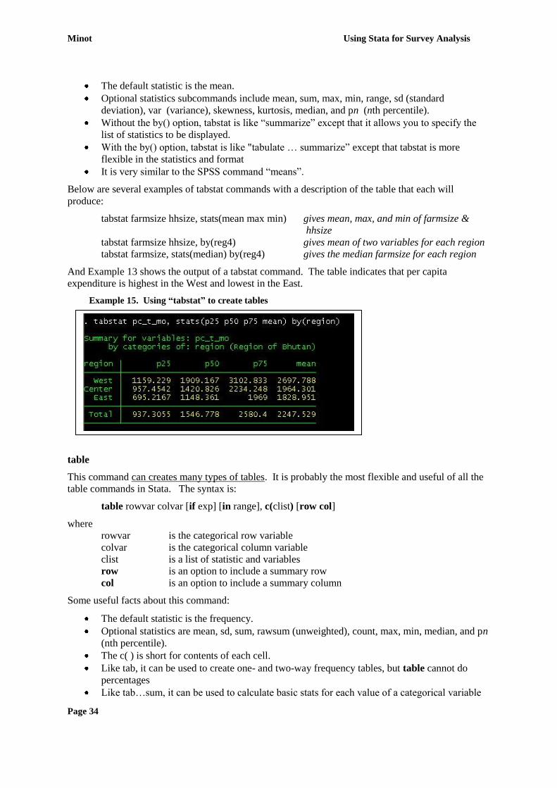
Minot Using Stata for Survey Analysis
Page 34
The default statistic is the mean.
Optional statistics subcommands include mean, sum, max, min, range, sd (standard
deviation), var (variance), skewness, kurtosis, median, and pn (nth percentile).
Without the by() option, tabstat is like “summarize” except that it allows you to specify the
list of statistics to be displayed.
With the by() option, tabstat is like "tabulate … summarize” except that tabstat is more
flexible in the statistics and format
It is very similar to the SPSS command “means”.
Below are several examples of tabstat commands with a description of the table that each will
produce:
tabstat farmsize hhsize, stats(mean max min) gives mean, max, and min of farmsize &
hhsize
tabstat farmsize hhsize, by(reg4) gives mean of two variables for each region
tabstat farmsize, stats(median) by(reg4) gives the median farmsize for each region
And Example 13 shows the output of a tabstat command. The table indicates that per capita
expenditure is highest in the West and lowest in the East.
Example 15. Using “tabstat” to create tables
table
This command can creates many types of tables. It is probably the most flexible and useful of all the
table commands in Stata. The syntax is:
table rowvar colvar [if exp] [in range], c(clist) [row col]
where
rowvar is the categorical row variable
colvar is the categorical column variable
clist is a list of statistic and variables
row is an option to include a summary row
col is an option to include a summary column
Some useful facts about this command:
The default statistic is the frequency.
Optional statistics are mean, sd, sum, rawsum (unweighted), count, max, min, median, and pn
(nth percentile).
The c( ) is short for contents of each cell.
Like tab, it can be used to create one- and two-way frequency tables, but table cannot do
percentages
Like tab…sum, it can be used to calculate basic stats for each value of a categorical variable

Using Stata for Survey Data Analysis Minot
Page 35
Its advantagehead over tab…sum is that it can do more statistics and it can take more than
one continious variable
Like tabstat, it can be used to calculate advanced stats for each value of a categorical variable
Its advantage over tabstat is that it can use do two- and three-way tables, but its disadvantage
is that it has fewer statistics.
It is similar to “table” in SPSS, but much easier to learn. On the other hand, it is less flexible
than the “table” command in SPSS.
Here are some examples:
. table region, row table of number of households in each
region, with a total row
. table region, c(mean pcexpend) table of average pcexpend by region
. table region, c(mean yield sd yield median yield) table of yield statistics by region
. table region, c(mean yield) format(%9.2f) table of average yields by region with format
. table region sexhead, c(mean yield) table of average yield by region and sex
. table region c(mean pcexpend mean yield) table of avg yield & pcexpend by region
The box below shows the output of three table commands. The first table shows the mean household
size in each region and in each stratum (urban and rural). The option format(%4.1f) means fixed
format with 4 digits and one to the right of the decimal point. The second table shows the mean per
capita expenditure for each region and for male and female-headed households. The option
format(%7.0fc) means that seven digits should be displayed, but none to the right of the decimal
period, in fixed comma format. The third table shows the mean household size and per capita
expenditure in each region.
Example 16 Using “table” to create tables

Minot Using Stata for Survey Analysis
Page 36
Using weights
What are sampling weights? Sampling weights are used to compensate for under- or over-
representing certain households in a sample, allowing it to reflect the population as a whole. Let‟s
take a simple example:
Suppose there are 200,000 households in the population, of which 160,000 live in rural areas.
A survey is carried out with a random sample of 2000 urban households and 2000 rural
households. Thus, the population is 80% rural but the sample is only 50% rural.
Suppose per capita income is 2800 in urban areas and 1400 in rural areas. The simple average
income across households in the sample would be 2100, but we know that the average income
across the country would be lower than this because rural households (who have lower
incomes) are under-represented in the sample.
We can compensate for this by using a weighted average, with weights equal to the ratio of
the population to the sample. The urban weight would be 20 (=40 thousand/2 thousand) and
the rural weight would be 80 (=160 thousand/2 thousand). The weighted average is
calculated as (80*1400 + 20*2800)/(20+80) = 0.8*1400 + 0.2*2800 = 1680.
The basic principle is that the sampling weight is the inverse of the probability of selection. Because
of clustering and sampling, virtually all random-sample surveys must use weights to make estimates
that are valid for the whole population. Furthermore, the calculation of sums, average, and
percentages must take into account the sampling weights.
Sampling weights in the BLSS The calculation of the sampling weights in the BLSS is more
complicated than the example given above, but the principle is the same. The NSB divided the
country into seven strata:
Thimphu
other urban areas in the west
urban areas in the center
urban areas in the east
rural areas in the west
rural areas in the center, and
rural areas in the east.
In each urban stratum, the NSB selected 60 blocks and about 10 households in each block, while in
each rural stratum, NBS selected 30 geogs and interviewed about 20 households in each geog (some
adjustments were necessary in implementation). Since more than half the BLSS sample is urban, it is
clear that urban areas were over-sampled (this is common practice in household surveys, based on the
idea that urban households are more diverse). In the BLSS, the sampling weight is called “weight” in
the file households.dta. The average value of “weight” is about 10 in urban areas: this means that the
BLSS interviewed about 10% (1/10) of the urban households and that each sample household
“represents” about 10 households in the urban population. The average value of “weight” in rural
areas is about 49. This implies that the BLSS interviewed about 2% (=1/49) of the rural households
and that each sample household “represents” 49 households in the rural population.
Using sampling weights in Stata The calculation of weighted sums and weighted average would be
very tedious, but fortunately survey software such as SPSS and Stata do this for us. In SPSS, you
turn on the weights and weights are used in all calculations until you turn it off. Stata is different in
that you tell Stata which commands should use weights.
Stata allows four kinds of weights:
1) fweights, or frequency weights, are weights that indicate the number of duplicated
observations.

Using Stata for Survey Data Analysis Minot
Page 37
2) pweights, or sampling weights, are weights that denote the inverse of the probability that the
observation is included due to the sampling design.
3) aweights, or analytic weights, are weights that are inversely proportional to the variance of an
observation;
4) iweights, or importance weights, are weights that indicate the "importance" of the observation
in some vague sense.
Here we will focus on pweights and fweights. The syntax for using weights is:
command ... [weight_type=varname] ...
In the case of the BLSS, we will generally be using the following syntax:
command … [aw=wt] …
Here are some examples:
tab region [aw=weight] gives the weighted frequencies in each region
sum hh_size [aw=wt] gives the weighted mean household size
tab b21_q1 [aw=wt], sum(pc_t_mo) gives table of weighted mean expenditure by sex of
head of household
tabstat hhsize [aw=weight], by(stratum) gives the weighted average household size for urban
and rural households
Example 17 shows the effect of weights. The first table gives the unweighted percentage of urban and
rural households in the sample. In the second table, the weights are turned on, showing the estimated
proportions in the country. Notice that the urban households represent almost 58% of the sample just
23% of the population. The third table confirms that the rural weights are larger than the urban
weights.
Type “help weights” in the Stata Command window for more information.
Example 17. Using weights in generating tables
Minot Using Stata for Survey Analysis
Page 38
SECTION 8: MODIFYING DATA FILES
This section describes a number of commands that are used to modify and combine data files in Stata.
We begin with a five simple commands and then move to five more complex ones.
rename
drop
keep
sort
compress
collapse
merge
append
reshape
fillin
rename
This command renames variables. Some examples:
rename oldname newname
rename b21_q1 sexhead
rename b21_q3ag agehead
drop
This command deletes records or variables. Examples are:
drop if agehead>140 deletes records in which age is greater than 140
drop if area==. deletes records in which area is missing
drop temp1 temp2 deletes variables temp1 and temp2
keep
This command deletes everything but specified observations or variables. Examples include:
keep if agehead <= 140 keeps only records in which age is 140 or under
keep hhid agehead pcexpend keeps only variables hhid, agehead, and pcexpend,
deleting all others
sort
This command sorts the records in the file according to the value of specified variables. It is the same
as “sort cases” in SPSS. Examples are:
sort region town sorts data file in order of region and town
sort urban sorts by the dummy variable urban
compress
This command reduces the size of the file by changing the data storage types. It will not make any
changes that would cause Stata to lose data. This command has no options or arguments.

Using Stata for Survey Data Analysis Minot
Page 39
collapse
This command is used to create a new data file by aggregating the existing one. It allows you to
change the level of the data file. Person-level data can be collapsed to the household level to calculate
the size of the household. Crop–level data, for instance, can be collapsed to the household-level to
calculate the value of agricultural production per household. The syntax is:
collapse (stat1) varlist1 (stat2) varilist2, by(varlist3)
where
stat1 refers to a statistic such as sum, mean, maximum or minimum
varlist1 are the variables to be aggregated using the first statistic
stat2 refers to a second statistic (optional)
varlist2 are the variables to be aggregated using the second statistic (optional)
varlist3 are the categorical variables which define the aggregation
Some points about the collapse command:
The default statistic is mean
Optional statistics are mean, sum, rawsum, count, max, min, median, and pn (the nth
percentile, where n is between 1 and 100)
The output file will have one record for each value of varlist3 in the by( ) option
If no by( ) option is given, then the data will be collapse to one record
This is similar to “aggregate” in SPSS except Stata does not require you to define a new name
for the aggregated variable (by default, it uses the old variable name).
Examples of the collapse command:
collapse agehead educ pcexpend, by(region) creates a dataset of provincial
means of age, education, and
pcexpend
collapse (median) pcexpend, by(region) creates a dataset of provincial
medians of pcexpend
collapse (mean) agehead (median) pcexpend, by(region) creates a dataset of regional means
of age and regional medians of
pcexpend
In Example 18, we use a different BLSS data file called “food expenditure.dta.” This file has
information on the value and source of food consumed by each household. It is at the household-food
type level, meaning that each observation has data on one food type for one household. The first
“sum” command shows that there are about 60 thousand observations in the file, which implies that
there are about 15 observations on average for the 4007 households in the BLSS. It also shows that
the average value of consumption is BTN 2274 per year per food type per household. Suppose we
want to calculate the average value of food consumption per household. We use the collapse
command to generate a household-level file with total value of food consumption for each household.
After the collapse, the second sum command indicates that there are just 4007 records, one per BLSS
household. It also shows that the average (unweighted) value of food consumption is BTN 34,835 per
year per household.

Minot Using Stata for Survey Analysis
Page 40
Example 18. Using “collapse” to calculate the value of food consumption per household
merge
This command combines two files with different variables into one file. Until now, all the commands
we have worked with used just one file. However, the BLSS consists of many data files, and often we
would like to combine data from different files. For example,
to calculate total expenditure, we would need to combine data from Block 8 (food
consumption) and Block 9 (non-food consumption).
to see if food consumption patterns vary depending on the education level of the head of
household, we need to combine data from Block 2.2 (education) and Block 8 (food
consumption).
The merge command combines files horizontally (side to side). In this case, the two files have
different variables and are linked by having the same observations (person, household, crop, etc.)
The files below have different variables but the same records (household). The command merge will
combine records with the same household identification number (hhid). This would allow an analysis
of how housing value (in the second file) varies according to expenditure level (in the first).
Two files before merge
hhid region urban exppc quint farm hhid housetype water elect value
101 101
102 102
103 103
201 201
202 202
203
║
║
▼
One file after merge
hhid region urban exppc quint farm housetype water elect value
101
102
103
201
202
203
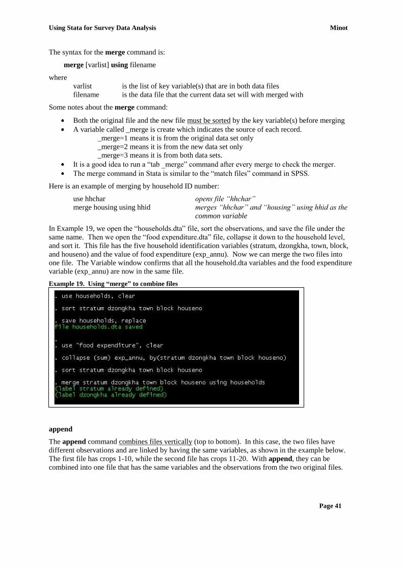
Using Stata for Survey Data Analysis Minot
Page 41
The syntax for the merge command is:
merge [varlist] using filename
where
varlist is the list of key variable(s) that are in both data files
filename is the data file that the current data set will with merged with
Some notes about the merge command:
Both the original file and the new file must be sorted by the key variable(s) before merging
A variable called _merge is create which indicates the source of each record.
_merge=1 means it is from the original data set only
_merge=2 means it is from the new data set only
_merge=3 means it is from both data sets.
It is a good idea to run a “tab _merge” command after every merge to check the merger.
The merge command in Stata is similar to the “match files” command in SPSS.
Here is an example of merging by household ID number:
use hhchar opens file “hhchar”
merge housing using hhid merges “hhchar” and “housing” using hhid as the
common variable
In Example 19, we open the “households.dta” file, sort the observations, and save the file under the
same name. Then we open the “food expenditure.dta” file, collapse it down to the household level,
and sort it. This file has the five household identification variables (stratum, dzongkha, town, block,
and houseno) and the value of food expenditure (exp_annu). Now we can merge the two files into
one file. The Variable window confirms that all the household.dta variables and the food expenditure
variable (exp_annu) are now in the same file.
Example 19. Using “merge” to combine files
append
The append command combines files vertically (top to bottom). In this case, the two files have
different observations and are linked by having the same variables, as shown in the example below.
The first file has crops 1-10, while the second file has crops 11-20. With append, they can be
combined into one file that has the same variables and the observations from the two original files.

Minot Using Stata for Survey Analysis
Page 42
Two files before append One file after append
hhid crop area quant value hhid crop area quant value
101 1 101 1
101 4 101 4
102 1 102 1
102 7 102 7
103 2 103 2
══► 101 16
hhid crop area quant value 102 12
101 16 102 13
102 12 103 11
102 13 103 16
103 11 103 19
103 16
103 19
The syntax for this command is:
append using filename
where filename is the name of the file to be added to the current data set. This command is similar to
“join files” in SPSS.
None of the sample files from the BLSS need to be appended, but here are several situations where
you might need to append files:
The housing data from a survey were entered by three different people, each creating a separate
file. You can use append to put them into one housing file with the following commands:
use housing1, clear
append using housing2
append using housing2
You have 20 files, each containing the crop data for one of the dzongkhags. You can use append
to combine them into one file.
A survey has crop production data for annual food crops, annual industrial crops, and tree crops in
three files. You can use append to combine the three files into one crop file.
In all three cases, the different files to be combined must have different observations but the same
variables.
fillin
This command inserts additional records into a file so that all combinations of two or more variables
are in the file. Again, it is easier to give an example than to describe it. Suppose we are working with
the food expenditure data. Data are collected on different food categories, but most households do not
consume all of them and records exist only for foods consumed by the household (this is how the
BLSS food expenditure data are organized). In the database below, there are five food categories but
each household only consumes 2-3 of them.

Using Stata for Survey Data Analysis Minot
Page 43
File in original form
hhid food quant value
1 1 3 3
1 3 1 1
1 5 1 1
2 1 1 1
2 5 1 1
3 1 2 2
3 4 1 1
3 5 4 4
If we calculate the average value for each food, it will give the average value among those consuming
the food. If we want the average value including the non-consumers, it is not easy to calculate. Stata
allows you to fill in the “missing” records of foods not consumed by each household. The syntax is
easy:
fillin varlist
where varlist is the list of variables, every combination of which we want to exist in the file. Using
our example above, the command would be
fillin hhid food
Stata will look for all the values of hhid and all the values of food in the file, then it will make sure
every hhid-food combination has a record. When it has to insert record, the values of the other
variables will be missing. The new file would look like this:
File after fillin command
hhid food quant value
1 1 3 3
1 2 . .
1 3 1 1
1 4 . .
1 5 1 1
2 1 1 1
2 2 . .
2 3 . .
2 4 . .
2 5 1 1
3 1 2 2
3 2 . .
3 3 . .
3 4 1 1
3 5 4 4
If we calculate the average value using this file, we will get the same answer as above. Because
missing values are not counted, the result will be the average among consumers. But if we replace the
missing values with zeros:
recode quant .=0
recode value .=0

Minot Using Stata for Survey Analysis
Page 44
then the average will include the zeroes. This is an extremely useful command, particularly for
dealing with food consumption, expenditure, and crop production data. SPSS does not have a similar
command.
reshape
The command changes a file from tall to wide or from wide to tall. What do we mean by “wide” and
“tall”? A wide file stores additional information as separate variables, while a tall file stores this
information using additional records. An example will be easier to understand. Food expenditure
data includes different types of foods and the value of expenditure on each. One way to store this data
is with a wide file, in which additional loans are stored in additional variables.
File in “wide” format
hhid food1 value1 food2 value2 food3 value3
1
2
3
4
5
The other way to store the data is with a tall file, in which each food item is stored as separate
observation.
File in “tall” format
hhid food value
1 1
1 2
1 3
2 1
2 2
2 3
3 1
3 2
3 3
4 1
4 2
4 3
5 1
5 2
5 3
Notice that both files have the same number of data points (30) for food type and value, they are just
arranged differently. The reshape command allows you to convert one type of file into the other. For
more information, type “help reshape” in the Stata Command window. For information on how to
implement reshape, type “help reshape.”
Using Stata for Survey Data Analysis Minot
Page 45
SECTION 9: PRESENTING DATA WITH GRAPHS
This section provides a brief introduction to creating graphs. In Stata, graphs are primarily made with
the graph command, followed by numerous subcommands for controlling the type and format of
graph. In addition to graph, there are many other commands that draw graphs. In this section, we
focus on four types of graph and a few options. These are the commands and subcommands covered
in this section:
graph
twoway
bar
pie
matrix
connect( )
msymbol( )
histogram
scatter
graph
This command generates numerous types of graphs and diagrams. The syntax is:
graph graphtype [varlist] [if exp] [in range] [, options]
where
graphtype is the type of graph
varlist is the list of variables to graph
if is used to limit observations that are included based on the exp condition
in is used to limit observations that are included based on the case number
options are commands to control the look of the graph
The main graph types drawn with the graph command are:
twoway Two-way graphs with two variables
matrix Matrix of two-way scatter-plot graphs
box Box-and-whisker plot
dot Dot chart
bar Bar chart of means or sums
pie Pie chart
Other graphs
Two commonly used graph types work as separate commands:
histogram Bar chart based on frequency
scatter Scatter plots based on two variables
histogram
This command generates a histogram, a bar chart showing the distribution of values of one variable.
The syntax is:
histogram varname [if exp] [in range] [weight] [, [continuous_opts | discrete_opts] options]
where
Minot Using Stata for Survey Analysis
Page 46
varname is the name of the variable to be graphed
if is used to limit observations that are included based on the exp condition
in is used to limit observations that are included based on the case number
weight is to give the weighted distribution
options are commands to control the look of the graph
scatter
This command generates a two-way scatter plot, showing a dot for each observation. The syntax is:
scatter varlist [if exp] [in range] [weight] [, options]
where
varlist is the list of variables to be graphed
if is used to limit observations that are included based on the exp condition
in is used to limit observations that are included based on the case number
weight is to give the weighted distribution
options are commands to control the look of the graph
graph options
There are too many options to describe here, but we describe how to make some of the more common
graphs.
Some options are common to many graph types:
title(“text”) specifies the title to use on the graph
xti(“text”) specifies title on X axis
yti(“text”) specifies title on Y axis
by(var1) repeat graph for each value of var1
Some options for histograms:
bin(#) specifies that the histogram will have # bars (# is a number)
freq label Y axis in terms of frequency
percent label Y axis in terms of percent
normal draws a normal curve with the means and standard deviation of the variable
Some options for two-way scatterplots:
connect( ) to specify how points are connected
msymbol( ) to specify what the marker look like
Some options for bar charts:
over(var1) plot y-variable for each value of var1 in one graph
stack stack the bars for each variable rather than putting them side by side
Here are some examples of the histogram, scatter, and graph commands:
histogram x histogram of x
histogram x, bin(5) histogram with 5 bars
scatter y1 y2 x scatter plot of y1 and y2 against x
scatter y x, by(region) scatter plots of y against x for each region
graph bar a b c bar graph of the means of a, b, and c
graph bar (sum) a b c bar graph of the sums of a, b, and c s
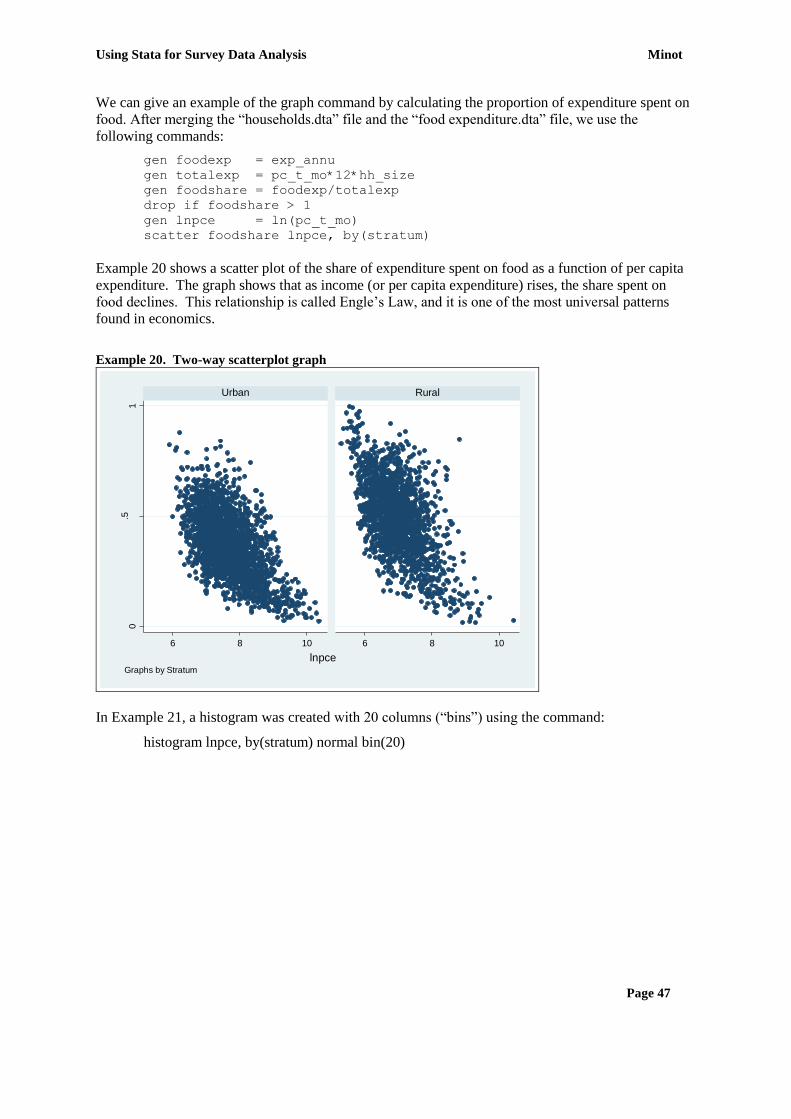
Using Stata for Survey Data Analysis Minot
Page 47
We can give an example of the graph command by calculating the proportion of expenditure spent on
food. After merging the “households.dta” file and the “food expenditure.dta” file, we use the
following commands:
gen foodexp = exp_annu
gen totalexp = pc_t_mo*12*hh_size
gen foodshare = foodexp/totalexp
drop if foodshare > 1
gen lnpce = ln(pc_t_mo)
scatter foodshare lnpce, by(stratum)
Example 20 shows a scatter plot of the share of expenditure spent on food as a function of per capita
expenditure. The graph shows that as income (or per capita expenditure) rises, the share spent on
food declines. This relationship is called Engle‟s Law, and it is one of the most universal patterns
found in economics.
Example 20. Two-way scatterplot graph
0.5
1
6 8 10 6 8 10
Urban Rural
foo
dsh
are
lnpceGraphs by Stratum
In Example 21, a histogram was created with 20 columns (“bins”) using the command:
histogram lnpce, by(stratum) normal bin(20)

Minot Using Stata for Survey Analysis
Page 48
Example 21. Histogram of per capita expenditure in Bhutan
0.2
.4.6
4 6 8 10 4 6 8 10
Urban Rural
Density
normal lnpce
Den
sity
lnpce
Graphs by Stratum
In Example 22, the bar graph of average per capita expenditure by stratum (urban/rural) and by sex of
head of household was created using the command:
graph bar pc_t_mo, over(b21_q1) over(stratum)
Example 22. Bar chart of per capita expenditure by region
0
1,0
00
2,0
00
3,0
00
4,0
00
me
an
of pc_
t_m
o
Urban Rural
Male Female Male Female
Using Stata for Survey Data Analysis Minot
Page 49
SECTION 10: REGRESSION ANALYSIS
This section describes the use of Stata to do regression analysis. Regression analysis involves
estimating an equation that best describes the data. One variable is considered the dependent
variable, while the others are considered independent (or explanatory) variables. Stata is capable of
many types of regression analysis and statistical tests. In this section, we touch on only a few of the
more common commands and procedures. The commands described in this section are:
regress
probit
predict
test, testparm
ovtest
hettest
svy option
regress
This command carries out a regression analysis on the variables specified. Regression analysis
estimates an equation of “independent” (or “explanatory”) variables that best explains variation in a
“dependent” variable. This command is used when the dependent variable is a continuous variable.
The syntax is:
regress depvar varlist [if exp] [in range] [options]
where
depvar is the dependent variable
varlist is the list of independent variables
The regress command has many options for specifying the type and format of the output. Type “help
regress” for more information. Some examples of the command:
regress y x1 x2 x3 x4 x5 regress y with x’s as independent variable
regress y x1 x2 x3 x4 x5 if region==1 same regression but only in one region
by region: regress y x1 x2 region* region* means all variables starting with region
Example 23 presents the results of a regression analysis of the determinants of food expenditure using
the merged data from the household.dta file and the food expenditure.dta file. The dependent variable
is the log of food expenditure per capita. The explanatory variables include the log of per capita
expenditure, stratum (whether or not the household is in an urban area), the household size, the sex of
the head of household, and two dummies to represent the west and central regions. For each
explanatory variable, the output includes six columns:
Coefficient: The effect of a one unit change in the explanatory variable on the
dependent variable.
Standard error A measure of the accuracy of the estimate of the coefficient
t statistics The coefficient divided by the standard error. Generally, any t
statistics greater than 2 is considered statistically significant.
P > |t| The probability that the coefficient is actually zero, given the data.
Any value of P less than .05 is considered statistically significant
95% confidence interval Two columns showing the lower and upper limit of 95% confidence
interval. This means the data indicate that we can be 95% sure that
the true value lies between the upper and lower limit.

Minot Using Stata for Survey Analysis
Page 50
The results in Example 23 indicate that food expenditure rises with per capita expenditure, that is
high-income people spend more on food than low-income people. Because both food expenditure and
per capita total expenditure are expressed in logs, the coefficient is the income elasticity of food. In
other words, a 1% increase in income (per capita expenditure) is associated with a 0.47 percent
increase in food expenditure. The fact that the elasticity is less than one means that food expenditure
rises more slowly than total expenditure, so the share of expenditure on food falls as income rises.
In addition, rural households spend somewhat more on food than urban households, after controlling
for other factors. The positive coefficients on reg_1 and reg_2 indicate that households in the west
and center spend more on food than households in the east. The t statistic in the sexhead is just 0.14,
smaller than 2, so we can say that the effect of sex of head of household on food expenditure is
statistically insignificant. Finally, larger households spend less on food, holding other factors
constant.
Example 23. Using “regress” to examine determinants of meat expenditure
probit
This command carries out a probit regression analysis of the specified variables. The syntax is:
probit depvar indepvars [if exp] [in range] [, options]
Probit analysis is used when the dependent variable is a binary variable (with only two values), such
as whether or not a household is poor. An alternative is the dprobit command which reports the
derivative of the probability with respect to each independent variable instead of the coefficient.
Examples include:

Using Stata for Survey Data Analysis Minot
Page 51
probit y x1 x2 x3 run a probit with y as dependent and x’s as independent
probit x1 x2 x3, robust run a “robust” probit (weaker assumptions about error)
dprobit y x1 x2 x3 if reg4 ==1 run the probit in one region only
predict
This command can be used to obtain predictions, residuals, etc., after regression analysis.
predict newvarname [if exp] [in range] [, options]
Two of the most common options are:
xb predicted values of y are put in newvarname
e residuals of the regression are put in newvarname
For example:
regress y x1 x2 x3
predict yhat, xb creates variable yhat with predicted values
predict e, resid creates variable e with residuals
probit poverty agehead sexhead housing
predict index, xb creates variable index with the value of sum of XB
predict phat creates variable phat with the predicted probability
test
This command tests hypotheses about the estimated parameters from the most recently estimated
model. For example,
regress y agehead female educ region1 region2 region3 region4
test region1=region2 test hypothesis that region1 coef = region2 coef
test educ=.1 test hypothesis that educ = 0.1
test region1 region2 region3 region4 test of hypothesis that four region dummies are zero
If you want to test the hypothesis that a set of related variables are all equal to zero, you can use the
related testparm command:
testparm region* test of hypothesis that all region* dummies are zero
ovtest
Regression analyis generates the best unbiased linear estimates of the “true” coefficients provided that
some assumptions are satisfied. One assumption is that there are no missing variables that are
correlated with the error term. This command performs a Ramsey RESET to test for omitted
variables (misspecification). The syntax is:
ovtest [, rhs]
This test is the same as estimating y = xb+zt+u and then testing t=0. If the rhs option is not specified,
powers of the fitted values are used for z . Otherwis, the powers of the indiependent variables are
used.. Examples of the test are:
regress y x1 x2 x3
ovtest tests significance of powers of predicted y
ovtest, rhs tests significance of powers of x1, x2, and x3

Minot Using Stata for Survey Analysis
Page 52
hettest
Another assumption behind regression analysis is that the variance of the error term is constant across
the sample. When this assumption is violated, the problem is called heteroskedasticity. This
command tests for heteroskedasticity.
hettest [varlist]
This command tests t=0 in Var(e)=s^2exp(zt). If varlist is not specified, the fitted
values are used for z. If varlist is specified, the variables specified are used for z.
This test is also known as the Breusch-Pagan test for heteroskedasticity. Examples are:
regress y x1 x2 x3
hettest test whether variance related to predicted y
hettest x3 test whether variance related to x3
Example 24 gives the result of some tests related to the regression analysis shown earlier. The
testparm command tests the hypothesis that both the region coefficients are equal to zero (that region
does not influence rice expenditure). The hypothesis is rejected, meaning that the regional
coefficients are jointly significant. The ovtest rejects the hypothesis that there are no omitted
variables, indicating that we need to improve the specification (prices would be a good start). And
finally, hettest indicates that there is heteroskedasticity which needs to be addressed.
Example 24. Using “test” to test hypotheses
svy option
The svy option is used with many statistical commands (including regress and probit) to adjust for the
effect of sample design when analyzing survey data. Most surveys are based on stratified cluster
samples rather than pure random samples. In Section 7, we saw that the sample design affects the
calculation of averages and percentages, so we need to calculate weighted averages and percentages to
compensate for the fact that some households are over-represented in the sample, while others are
under-represented. The sample design also affects the calculation of standard errors in regression
analysis. It does this in two ways:

Using Stata for Survey Data Analysis Minot
Page 53
Stratification: The goal of stratification is to over-represent groups of households that are highly
diverse in the variables of interest (e.g. income). If well done, stratification therefore increases the
accuracy of estimates (that is, it reduces the standard errors) compared to a simple random
sample.
Clustering: The goal of using clusters of households in samples is to reduce the cost of data
collection, but this reduces the accuracy of estimates (that is, it increases the standard error)
compared to a non-clustered random sample. To see this, imagine the difference between
interviewing 100 households dispersed across the country and interviewing 100 households in one
village. Clearly, estimates based on the latter would be less accurate.
The svyset command is used to describe the sample design. Then the svy: prefix is used before other
commands such as regress and probit. The syntax for svyset is organized according to each level in
the sample design.
In the case of the BLSS, for example, we need to first define the primary sampling unit. The primary
sampling unit is the block (in urban areas) or geog/town in rural areas, so we define the variable “psu”
to be equal to the block number in urban areas and the town/geog number in rural areas (first two
commands below). Next, we define the seven strata used for the BLSS (second two commands
below). Third, in the svyset command, we specify the primary sampling unit variable (psu), and the
sampling weight variable (weight), the strata variable (strata7). The two vertical lines followed by _n
indicate that in the second stage, the sampling was random.
gen psu = block if stratum==1
replace psu = town if stratum==2
gen strata7 = 10*stratum + region
replace strata7 = 10 if dzongkha==14 & stratum==1
svyset psu [pw=weight], strata(strata7) || _n
There is also a finite population correction if the number of units sampled is large compared to the
total number of units. For more information, type “help svyset” in the Stata Command window.
Once the sample design has been set, it can be used to run regression analyses that take the sample
design into account:
svy: regress y x1 x2 x3 x4 x5
svy: probit y x1 x2 x4 x4 x5
Example 25 shows the effect of adjusting for sampling design on the regression results. Compared to
the regression results in Example 23, the standard errors here are higher and the t statistics are lower.
The stratum (urban/rural) variable that was significant before is no longer significant after the
sampling method adjustments are made.
If the data set is saved after an svyset command, the sample design is saved with the data and is
available for use whenever the data are used in the future. The ability to correct for complex sample
designs in analyzing survey data is an important advantage of Stata.
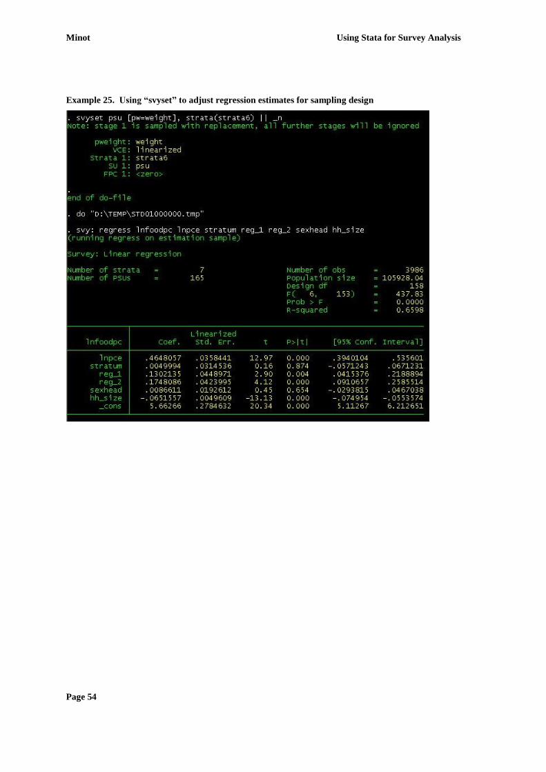
Minot Using Stata for Survey Analysis
Page 54
Example 25. Using “svyset” to adjust regression estimates for sampling design
Using Stata for Survey Data Analysis Minot
Page 55
SECTION 11: INTRODUCTION TO PROGRAMMING WITH STATA
This section provides a very quick introduction to the topic of programming with Stata. We touch on
three topics:
creating and using macros
creating and using loops
matrix algebra
The purpose here is not to provide a comprehensive description of how to program with Stata, but
rather to give you an idea of the kinds of things that can be done with Stata. To fully describe Stata
programming would require more space than is available here. In fact, it fills an entire book in the
Stata manuals.
Using macros
Macro assign a set of word or a number to a name. There are two types of macros.
“Global” macros stay in memory until you leave Stata
“Local” macros exist only with a program or a loop
The syntax is relatively simple:
global gmname = “ expression “
local lmname = “ expression “
To use these macros later, you must use special symbols to tell Stata they are macros:
$gmname
`lmname‟
One use of the global macro is to store the name of the folder with the data.
global path = “d:\Bhutan\2003 BLSS\Stata”
use “$path\food expenditure.dta”, clear
In addition to saving you some time, this macro is useful if you share the program with others who
have different names for the folders on their computer. By using the macro, your colleague can
change the global command once rather than trying to change the path in every command that opens a
file or saves a file.
Local macros are used (among other places) in loops with the while command, so we will discuss
them in the next section.
Using loops
This command starts a loop, allowing groups of Stata commands to be repeated until some condition
is met. The syntax is:
while exp {
commands
}
where exp is an expression. Stata repeats the commands as long as the expression is
true.
commands are any Stata commands that you want to repeat
{ } define the beginning and the ending of the commands to be repeated

Minot Using Stata for Survey Analysis
Page 56
This is an example of a loop that uses local macros to carry out a regression analysis of the
determinants of housing value for each region:
tab region, gen(reg_)
local r = 1
while `r' <= 4 {
regress housval roof floor wall room area water if reg_`r' == 1
local r = `r' + 1
}
The tab command creates a dummy variables for each region (region1, region2, etc). The first local
command creates a macro called “r” that is equal to 1. The while statement says that the commands
in brackets will be repeated until the condition r<=4 is no longer true. On each loop, the regress
command is carried out in one region (when r=3, the if statement is “if reg_3==1). The second local
command increases the value of r each time that the loop is completed. When r reaches 5, the loop
stops because the while condition is no longer true. Then Stata goes on to the next command after the
bracket.
Using matrix algebra
Stata has a special set of commands for matrix algebra. These can be used to implement custom
econometric procedures or for doing calculations on the output of regression analysis. This is a very
short summary of a very long list of complex commands. complex set of commands (type “help
matrix” for more information).
1. Creating matrices by hand
Examples:
matrix mymat = (1,2\3,4) commas separate elements, backslash indicates new row
matrix myvec = (1 5 3 1 3) creates a row vector
matrix mycol = (1/5/3/1/3) creates a column vector
2. Setting the maximum matrix size
For regular Stata, the default maximum matrix size is 40x40, but this can be increased up to 800x800
with the matsize command. For Stata SE, the default maximum is 400x400, but this can be increased
up to 11,000x11,000. The maximum matrix size can be changed using
set matsize 500 sets the maximum size for a matrix at 500x500
3. Manipulating matrices
Examples:
matrix D = B makes matrix D equal to matrix B
matrix beta = syminv(X'*X)*X'*y calculates beta using regression equation
matrix C = (C+C')/2 redefines C matrix in terms of old values
matrix sub = A[1..., 2..5]/2 defines matrix using sub-set of A matrix
matrix A[2,2] = B redefines subset of A matrix as equal to B
4. Converting variables into matrices and vice versa
Variables can be converted into matrices and likewise matrices can be converted into variables. Type
“help mkmat” for more information.

Using Stata for Survey Data Analysis Minot
Page 57
5. Using matrices created by Stata
Some Stata commands create matrices which can be retrieved and used. For example, all the
regression commands create the following:
e(b) coefficient vector
e(V) variance-covariance matrix of the estimates
And these matrices can be used as follows:
matrix beta = e(b) creates a vector called beta with the estimated coefficients
matrix cov = e(V) creates a matrix called cov with the estimated covariances
6. Accumulating cross-product matrices
Most statistical computations involve matrix operations such as X'X or X'WX. In many cases, X may
have a very large number of rows and a small number of columns. Stata has a special command for
calculating cross-products in these cases. Type “help matacum” for more information.
15. Matrix utilities
matrix dir lists the currently defined matrices
matrix list displays the contents of a matrix
matrix rename renames a matrix
matrix drop deletes a matrix

Minot Using Stata for Survey Analysis
Page 58
Annex 1: Quick reference guide to Stata commands
Command Description Command Description
Exploring data
cd
clear
use
describe
list
summarize
tabulate
tab1
tab2
save
help
bysort option
if option
in option
set more on
set more off
set mem XXm
set scrollbufsize
Storing commands and
output
scroll button
log using ..
log close
Creating new variables
gen
replace
operators
|
&
recode
tab …, generate
xtile
Making tables
label var
label def
label val
#delimit
tabulate … sum
tabstat
table
[pw = ]
change path
clear memory
open a data file
summarize file
list observations
summarize variables
make frequency table
make frequency table
make cross-tab table
save data file
get help on using Stata
repeat command
do if condition is true
do for selected records
output with pauses
non-stop output
set memory to XX Mb
set results window size
open Do-file Editor
start log of results
stop log of results
calculate new variable
redefine old variable
or
and
redefine values
create dummies
create terciles etc.
give label to a variable
define value labels
apply set of labels
set end-of-line symbol
table of statistics
table of statistics
table of statistics
use sampling weights
Graphs
graph
twoway bar
pie
matrix
histogram
scatter
Modifying files
drop
drop if
keep
keep if
sort
compress
collapse
merge
append
fillin
reshape
Regression analysis regress
probit
predict
test
testparm
ovtest
hettest
svyset
svy:
Programming
global
local
while
two-way graphs
bar charts
pie charts
matrix of scatter-plots
histogram graph
scatter plot
delete variables
delete records
keep variables
keep records
sort observations
reduce size of file
aggregate datafile
combine files horiz.
combine files vertically
insert missing rows
reshape datafile
run regression
run probit model
generate variables
test hypothesis
test hypotheses
test omitted variable
test heteroskedasticity
define sample design
adjust for sample des.
define global macro
define local macro
create loops to repeat

Using Stata for Survey Data Analysis Minot
Page 59
Annex 2: Comparison of SPSS and Stata commands
Description SPSS Stata
File manipulation
to open a file get file „filename‟. use “filename”
save a file save outfile „filename‟. save “filename”
[filename optional, add replace if
writing over old file]
combine files adding new variables match files /file filename /file
filename
/by varlist.
merge varlist using “filename”
[assumes you have one file open ]
combine files adding new records join files /file filename /file filename. append using “filename”
[assumes you have one file open]
aggregate file leaving fewer records aggregate outfile „filename‟
/break varlist /var = func(var).
collapse (func) varlist, by(varlist)
convert wide file format to long fomat
or vice versa
no equivalent command reshape wide var i(var) j(var)
reshape long var i(var) j(var)
sort records in file sort cases by varlist. sort varlist
select records for further processing sel if expression. keep if expression
Variable manipulation
create and define new variable compute var = expression. generate var = expression
redefine existing variable compute var = expression. replace var = expression
create aggregated variable in existing
file
no equivalent command,
must use aggregate and match files
egen var = function(varlist) by var1
change values of existing variable recode var (old=new) (old=new). recode varlist old=new old=new
Produce output
calculate an expression no equivalent command display expression
gives summary statistics on variables des varlist summarize varlist
lists values for each record for given
variables
list varlist. list varlist
gives frequency of each value of
variables
freq varlist. tab1 varlist
gives mean of first variable for each
value of second variable
mean var1 by var2.
tabulate var1, summarize(var2)
gives cros-tabulation crostab rowvarist colvarlist
[gives count by default, row and col
pct and other stats available]
tabulate rowvar colvar
[gives count by default, use row and col
to get percentages; other stats available]
tab2 varlist
[gives all 2-way tables]
creat a table (flexible format and
content) table table rowvar colvar c(func var) row col
[func can be n, sd, mean, etc]
Formatting and labeling
define format for variables format varlist format. format varlist (%format)
rename a variable rename oldvar newvar. rename oldvar newvar
give label to variable (eg region) variable label var „varname‟. label variables var1 “varname”.
give labels to values (eg Northern) value label 1 „label1' 2 „label2'. label define var1 lab 1 "lab" 2 "lab"
label values var1 var1lab
attach comments to variable or file no equivalent command notes var1 “comment”
notes “comment”


![New [SVY] Survey Datapublic.econ.duke.edu/stata/Stata-13-Documentation/svy.pdf · 2013. 6. 12. · Title intro — Introduction to survey data manual DescriptionRemarks and examplesAlso](https://static.fdocuments.us/doc/165x107/6045626b0da2e0044548e6b7/new-svy-survey-2013-6-12-title-intro-a-introduction-to-survey-data-manual.jpg)