Analyses using GLM - The University of Tennessee at ... · Web viewAnalyses Involving Only...

Analyses Involving Only Quantitative Factors

Example 1. Simple regression using GLM – predicting P5100 performanceData are valdat09.sav

Analyses Involving Quantitative Variables Using GLM - 1 9/22/3

Nominal Research factors (not group coding variables) go here.

Fixed Factors are those whose values represent the universe of possible values, such as Gender, Political Party.

Random Factors are those whose values represent a sample from the universe of possible values, such as Hospital or Work Group.

Continuous variables - the independent variables of traditional regression analysis - go here.

The Options I recommend are checked.

newform

Univariate Analysis of Variance

(The value of B, the slope, is .000447.)

Note that the Parameter Estimates box above gives you information not available in the REGRESSION output.But you also can get information from the REGRESSION Coefficients table that’s not in the above. Do both.


This output gotten by checking the “Parameter Estimates” box under Options. Note that the t for FORMULA is the square root of the F above.

Default Output. If you want output like that available in the Regression procedure, you have to obtain it from the "Parameter Estimates" box shown below.

This output gotten by checking the “Descriptive Statistics” box under Options.

This output gotten by checking the “Residual Plots” box under Options or /PLOT=RESIDUAL in syntax.

Example 2. Multiple Regression using GLM – Comparing validity of raw scores vs. percentile ranksA: Predicting core1st scores from UGPA, GREV, GREQ, and AW raw scores using GLM.

The core1st variable is the mean score (not grade) earned in the I-O core courses taught in the 1st year.It’s serving as the criterion in this validation study analysis. A better criterion would be scores in ALL the core courses across two years. I haven’t had the time to do that analysis. I don’t think the results would be much different than what follows.

The Output

UNIANOVA core1st WITH ugpa grev greq awrit /METHOD=SSTYPE(3) /INTERCEPT=INCLUDE /PRINT=OPOWER ETASQ DESCRIPTIVE PARAMETER /PLOT=RESIDUALS /CRITERIA=ALPHA(.05) /DESIGN=ugpa grev greq awrit.

Univariate Analysis of Variance[DataSet1] G:\MdbO\Dept\Validation\GRADSTUDENTS.sav


Relating the estimated coefficients to the formula coefficients:

Formula = 200*UGPA + 5*GREV + .5*GREQ

Ratio to Bugpa

---------------------Coef Formula Estimated Formula EstimatedBugpa 200 .070 1:1 1:1

Bgrev 0.5 .0003 1:400 1:265

Bgreq 0.5 .0003 1:400 1:200

This is the syntax that corresponds to the pull-down menu sequence illustrated above.

Descriptive Statistics

Dependent Variable: core1st Av of Z's of 506,512,516,(511+513)/2

Mean Std. Deviation N

-.0061 .78041 135

Tests of Between-Subjects Effects


Source Type III Sum of

Squares

df Mean Square F Sig. Partial Eta

Squared

Noncent.

Parameter

Observed Powerb

Corrected Model 26.896a 4 6.724 15.976 .000 .330 63.904 1.000

Intercept 23.102 1 23.102 54.889 .000 .297 54.889 1.000

ugpa 13.314 1 13.314 31.633 .000 .196 31.633 1.000

grev 2.524 1 2.524 5.998 .016 .044 5.998 .681

greq .641 1 .641 1.523 .219 .012 1.523 .232

awrit 3.495 1 3.495 8.303 .005 .060 8.303 .816

Error 54.715 130 .421

Total 81.616 135

Corrected Total 81.610 134

a. R Squared = .330 (Adjusted R Squared = .309)

b. Computed using alpha = .05

Note that all the predictors, with the exception of GREQ (!!!!!), contribute uniquely to the prediction of core1st. Although GREQ is always significant when PSY 5100 or PSY 5130 grades are the criterion, those courses were only about ¼ of the core1st variable. The other ¾ were from PSY 5160 (Training), PSY 5120 (Job Analysis) and PSY 5060 (Org Psych). I don’t believe any of these courses has a strong statistics/math emphasis. I need to speak to those professors.

R2 is .330, which means that R = .57. This is larger than the most of the validities reported in Schmidt & Hunter’s (1998) classic article on predictor validities. It’s particularly comforting given the fact that we’re working with a sample that exhibits restricted range.

The fact that the AWRIT test is uniquely significant validates ETS’s decision to add it to the GRE battery of tests – validates it at least for prediction of performance in our program.

Parameter Estimates


Parameter B Std. Error t Sig. 95% Confidence Interval Partial Eta

Squared

Noncent.

Parameter

Observed Powera

Lower Bound Upper Bound

Intercept -5.828 .787 -7.409 .000 -7.384 -4.272 .297 7.409 1.000

ugpa .991 .176 5.624 .000 .642 1.339 .196 5.624 1.000

grev .002 .001 2.449 .016 .000 .004 .044 2.449 .681

greq .001 .001 1.234 .219 -.001 .002 .012 1.234 .232


These are descriptive statistics on the dependent variable for all the groups specified in the analysis.

The mean is 0, since the dependent variable is a Z-score-like measure.

There is only one mean because there is only one group – no nominal (grouping) factors were specified.

!!!!!

awrit .254 .088 2.881 .005 .080 .429 .060 2.881 .816

a. Computed using alpha = .05

The B values are not too informative, although the fact that they’re all positive tells us that the relationships are in the expected directions. We would be given pause if one of the relationships was negative.


The plot of Observed vs. Predicted (circled) shows that the strong relationship was not due to outliers. If anything, the one possibly outlying point reduced R.


B: Predicting core1st scores from UGPA, GREV, GREQ, and AW percentile ranks using GLM.

This is an analysis of the same sample as in the previous analysis. The only difference is that percentile ranks, rather than raw scores, for the GRE tests were used. The reason for considering percentile ranks is to insulate us from any future changes in the GRE scoring system. The folks at ETS completely changed the scoring system for the GRE V and Q scores, from a mean=500, SD=100 to a mean=150,SD=10 system. This nullified our old formula score, and caused us to look for a way to avoid having to change it again, should ETS decide that mean=150, SD=10 was not going to work. I decided to look at percentile ranks, which don’t change as raw scores change as long as dimensions represented by the raw scores stay the same.

temporary.select if (p511yr <= 2011). Don’t have raw scores for 2012 students.UNIANOVA core1st WITH ugpa GREVPR GREQPR AWRITPR /METHOD=SSTYPE(3) /INTERCEPT=INCLUDE /PRINT=OPOWER ETASQ DESCRIPTIVE PARAMETER /PLOT=RESIDUALS /CRITERIA=ALPHA(.05) /DESIGN=ugpa GREVPR GREQPR AWRITPR.


[DataSet1] G:\MdbO\Dept\Validation\GRADSTUDENTS.sav


Dependent Variable: core1st Av of Z's of

506,512,516,(511+513)/2


-.0061 .78041 135




Squares


Squared

Noncent.

Parameter

Observed Powerb


Intercept 20.382 1 20.382 48.033 .000 .270 48.033 1.000

ugpa 14.190 1 14.190 33.441 .000 .205 33.441 1.000

GREVPR 3.220 1 3.220 7.589 .007 .055 7.589 .781

GREQPR .870 1 .870 2.051 .155 .016 2.051 .295

AWRITPR 2.668 1 2.668 6.287 .013 .046 6.287 .702

Error 55.162 130 .424

Total 81.616 135




The percentile rank prediction equation is not quite as valid as the raw score equation (R=.324 vs. R=.330), although I don’t believe the difference is significant. The pattern of “significances” is the same for the two analyses.


Parameter Estimates



Squared

Noncent.

Parameter

Observed Powera


Intercept -4.402 .635 -6.931 .000 -5.659 -3.146 .270 6.931 1.000

ugpa 1.020 .176 5.783 .000 .671 1.369 .205 5.783 1.000

GREVPR .008 .003 2.755 .007 .002 .014 .055 2.755 .781

GREQPR .005 .003 1.432 .155 -.002 .011 .016 1.432 .295

AWRITPR .006 .002 2.507 .013 .001 .011 .046 2.507 .702


The prediction equation is

Predicted core1st = 1.020*UGPA + .008*GREVPR + .005*GREQPR + .006*AWRITPR.

Multiplying everything by 100 . . .This is equivalent to 102.0*UGPA + .8*GREVPR + .5*GREQPR + .6*AWRITPR

This is roughly 100*UGPA + 1*GREVPR + 1*GREQPR + 1*AWRITPR which is what we’re using.


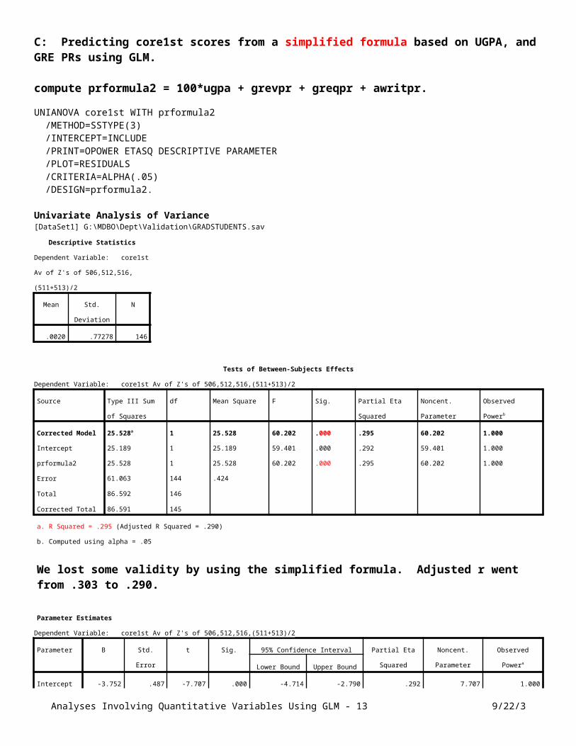
C: Predicting core1st scores from a simplified formula based on UGPA, and GRE PRs using GLM.

compute prformula2 = 100*ugpa + grevpr + greqpr + awritpr.

UNIANOVA core1st WITH prformula2 /METHOD=SSTYPE(3) /INTERCEPT=INCLUDE /PRINT=OPOWER ETASQ DESCRIPTIVE PARAMETER /PLOT=RESIDUALS /CRITERIA=ALPHA(.05) /DESIGN=prformula2.

Univariate Analysis of Variance[DataSet1] G:\MDBO\Dept\Validation\GRADSTUDENTS.sav


Dependent Variable: core1st Av of Z's

of 506,512,516,(511+513)/2


.0020 .77278 146




Squares


Squared

Noncent.

Parameter

Observed Powerb


Intercept 25.189 1 25.189 59.401 .000 .292 59.401 1.000

prformula2 25.528 1 25.528 60.202 .000 .295 60.202 1.000

Error 61.063 144 .424

Total 86.592 146




We lost some validity by using the simplified formula. Adjusted r went from .303 to .290.

Parameter Estimates



Squared

Noncent.

Parameter

Observed Powera


Intercept -3.752 .487 -7.707 .000 -4.714 -2.790 .292 7.707 1.000

prformula2 .008 .001 7.759 .000 .006 .010 .295 7.759 1.000



Aside: Convergent Validity of Personality QuestionnairesThis page is an aside. It was covered in PSY 5100. It’s FYI and an introduction to the analysis that follows.

The Big Five are five basic dimensions of normal personality.They are Extraversion, Agreeableness, Conscientiusness, Emotional Stability, and Openness to Experience.There are several questionnaires that measure the Big Five. One of the most popular is that called the NEO-FFI-3.

In the past 15 years, a group of psychologists has provided evidence for the existence of six basic dimensions.They are eXtraversion, Agreeableness, Conscientiousness, Emotional Stability, Openness to Experience and Honesty/Humility. There is one questionnaire that measures these six dimension, the HEXACO.

Note that five of the dimensions in the two questionnaires have the same name. The question addressed here is whether those with the same name exhibit convergent validity.

The data: 1195 students who responded to both the NEO-FFI-3 and the HEXACO-PI-R. The NEO is a 60-item questionnaire, 12 items per Big Five dimension. The HEXACO is a 100-item questionnaire, 16 items per dimension with 4 items representing a “filler” characteristic.

Cronbach alpha reliability estimates are in boldface on the diagonal. Convergent validity correlations are those in red. As can be seen, three of the measures – Extraversion, Conscientiousness, and Openness are measured similarly by the two questionnaires. Their convergent validities are nearly as large as their reliabilities. Most researchers would probably treat the two questionnaires as interchangeable with regard to those three dimensions.

But the HEXACO measures a different Stability than does the NEO. And the HEXACO measures a different Agreeableness than does the NEO. For these two dimensions, researchers have to decide which Stability they wish to measure and which Agreeableness they wish to measure.

Correlationsnx na nc ns no hx ha hc hs ho hh

nx Pearson .845 .298 .360 .376 .040 .781 .174 .185 -.052 -.026 .058na Pearson .298 .793 .339 .198 .184 .233 .532 .307 -.216 .105 .509nc Pearson .360 .339 .869 .370 .027 .326 .174 .763 -.003 -.048 .207ns Pearson .376 .198 .370 .826 -.114 .509 .348 .237 .444 -.023 .134no Pearson .040 .184 .027 -.114 .784 .035 .059 .077 -.086 .733 .118hx Pearson .781 .233 .326 .509 .035 .877 .251 .254 .077 .050 .069ha Pearson .174 .532 .174 .348 .059 .251 .830 .183 .181 .117 .325hc Pearson .185 .307 .763 .237 .077 .254 .183 .857 -.073 .043 .280hs Pearson -.052 -.216 -.003 .444 -.086 .077 .181 -.073 .823 .044 -.076ho Pearson -.026 .105 -.048 -.023 .733 .050 .117 .043 .044 .809 .145hh Pearson .058 .509 .207 .134 .118 .069 .325 .280 -.076 .145 809

OK, now back to regression analysis using GLM.


Example 3: Predicting Honesty/Humility scores from the NEO Big Five.Perhaps the HEXACO folks are all wrong. Perhaps Honesty/Humility is simply a combination of the Big Five, so that is’s completely predictable from the Big Five. If so, it’s not a separate dimension at all, it’s simply a composite of the existing Big Five dimensions.

To test the hypothesis that H/H is a real factor separate from the NEO Big Five, I regressed H/H scores onto the NEO Scale scores using both REGRESSION . . .

Model Summary

Model R R SquareAdjusted R

SquareStd. Error of the

Estimate1 .526a .277 .274 .67531a. Predictors: (Constant), no, nc, nx, na, ns

Coefficientsa

ModelUnstandardized Coefficients

Standardized Coefficients

t Sig.B Std. Error Beta1 (Constant) 1.835 .187 9.792 .000

nx -.132 .026 -.143 -5.085 .000na .517 .028 .511 18.752 .000nc .054 .026 .058 2.047 .041ns .060 .025 .069 2.452 .014no .035 .025 .035 1.393 .164

a. Dependent Variable: hh

and GLM.Tests of Between-Subjects Effects

Dependent Variable: hh

SourceType III Sum of Squares df

Mean Square F Sig.

Partial Eta Squared

Noncent. Parameter

Observed Powerb

Corrected Model

207.819a 5 41.564 91.140 .000 .277 455.702 1.000

Intercept 43.726 1 43.726 95.881 .000 .075 95.881 1.000nx 11.790 1 11.790 25.853 .000 .021 25.853 .999na 160.370 1 160.370 351.656 .000 .228 351.656 1.000nc 1.912 1 1.912 4.192 .041 .004 4.192 .534ns 2.742 1 2.742 6.013 .014 .005 6.013 .688no .885 1 .885 1.941 .164 .002 1.941 .286Error 542.234 1189 .456

Total 24232.496 1195

Corrected Total

750.053 1194

a. R Squared = .277 (Adjusted R Squared = .274)b. Computed using alpha = .05

Parameter EstimatesDependent Variable: hh

Parameter B

Std. Error t Sig.

95% Confidence IntervalPartial Eta Squared

Noncent. Parameter

Observed Powera

Lower Bound

Upper Bound

Intercept 1.835 .187 9.792 .000 1.468 2.203 .075 9.792 1.000nx -.132 .026 -5.085 .000 -.183 -.081 .021 5.085 .999na .517 .028 18.752 .000 .463 .571 .228 18.752 1.000nc .054 .026 2.047 .041 .002 .106 .004 2.047 .534ns .060 .025 2.452 .014 .012 .108 .005 2.452 .688no .035 .025 1.393 .164 -.014 .085 .002 1.393 .286a. Computed using alpha = .05


So, adjusted R2 is .255, which means that only about ¼ of the variance of H/H scores was predictable by the Big Five.

This leads me to conclude (along with Lee and Ashton, the HEXACO developers) that the H/H scale scores represent variation on a dimension that is different from any combination of dimensions of the NEO Big Five.

One thing this example illustrates is that any time you encounter a “new” personality characteristic, you should check to see whether or not it is simply a combination of already existing characteristics.


Analyses with Qualitative and Quantitative Variables

Three General situations involving Qualitative and Quantitative Factors . . .

1. Interest is on comparison of means of groups defined by Qualitative factors controlling for Quantitative factors. The quantitative factor is just there as a controlling variable.

I wish to compare the effectiveness of two training programs. I know that smarter people get better scores after training. There might be differences in intelligence between the participants in the two conditions of my research. So I wish to control for intelligence of the trainees when comparing the training programs.

What’s it mean to be a controlling variable? How would you feel if I said, “You mean nothing to me. You’re just a controlling variable. Quit crying!!” Name of a country song: “I’m just a controlling variable to you.”

In fact, variables that are controlling variables are real in every sense except our interest in them. That means we might not conduct the test of the main effect of a controlling variable. But we would include a controlling variable in the analysis when we test the main effects of variables we ARE interested in – that’s what “controlling for” is all about. Moreover, we should also test for the interaction of each variable with each controlling variable.Given that we’ve spent that much time with controlling variables, my recommendation is that we also test their main effects. In which case, we’re treated them exactly like we’ve treated every other variable.

2. Interest is on the relationship of the DV to the quantitative factors controlling for differences between groups. The different groups are just a nuisance.

I wish to assess the strength of the relationship of GPA to Conscientiousness. I have males and females in my study. Does GPA relate to Conscientiousness when controlling for Sex. Is the relationship the same for males as it is for females? Same questions for ethnic groups – Whites vs African-Americans vs Orientals vs Hispanics.

3. Interest is on both comparison of means and on the relationship of the DV to quantitative factors.


Example 1: Comparing Group means controlling for a Quantitative factor.Question: Who does better in the statistics course – I-O or RM students after controlling for formula score.

Data: VALDAT09 – data on 353 I/O and RM students in the Psych MS programs over nearly 15 years.

MS Program (prog= 1 vs. prog= 0) and Entering ability (newform) – the formula score used prior to 2010.Data are valdat09. N=353.

The analysis assessing both effects – formula and prog - using REGRESSION

Tests that must be made

1. Relationship of DV to prog.2. Relationship of DV to formula.3. Relationship of DV to interaction of prog and formula.

General Procedure to follow . . .

1) Test the significance of each interaction.2) If the interaction between two variables is NS, drop the interaction from further comparisons.3) Test main effects, i.e., individual variables controlling for all other main effects and significant interactions.

Specific Testing Sequence recommend if you’re using REGRESSION

1) Put all variables in the equation2) Remove the interaction variable(s).3) Add the interaction variable(s) back in and assess the significance of R2 change.4) Remove the first main effect variable(s).5) Add the first main effect variable(s) back in and assess the significance of R2 change.6) Remove the second main effect variable(s).7) Add the second main effect variable(s) back in and assess the significance of R2 change.

SPSS syntax for following this procedure using REGRESSION

compute prod = prog*newform. prod is the interaction variable.

regression variables = p511g newform prog prod /descriptives=default /statistics = default cha/dependent=p511g /enter newform prog prod /remove prod /enter prod/remove prog /enter prog/remove newform /enter newform.


Regression [DataSet3] G:\MDBO\Dept\Validation\Valdat09.sav

Descriptive StatisticsMean Std. Deviation N

p511g .8692 .08101 352newform 1180.54 94.960 352prog .84 .372 352prod 986.9114 446.14240 352

Variables Entered/Removeda

ModelVariables Entered

Variables Removed Method

1 prod, newform, progb

. Enter

2 .b prodc Remove3 prodb . Enter4 .b progc Remove5 progb . Enter6 .b newformc Remove7 newformb . Entera. Dependent Variable: p511gb. All requested variables entered.c. All requested variables removed.

Model Summary

Model RR

SquareAdjusted R

SquareStd. Error of the Estimate

Change StatisticsR Square Change

F Change df1 df2

Sig. F Change

1 .526a .277 .270 .06921 .277 44.336 3 348 .0002 .526b .276 .272 .06912 .000 .099 1 348 .753

3 .526c .277 .270 .06921 .000 .099 1 348 .7534 .526d .276 .272 .06912 .000 .128 1 348 .721

5 .526e .277 .270 .06921 .000 .128 1 348 .7216 .434f .188 .184 .07321 -.088 42.503 1 348 .000

7 .526g .277 .270 .06921 .088 42.503 1 348 .000a. Predictors: (Constant), prod, newform, progb. Predictors: (Constant), newform, progc. Predictors: (Constant), newform, prog, prodd. Predictors: (Constant), newform, prode. Predictors: (Constant), newform, prod, progf. Predictors: (Constant), prod, progg. Predictors: (Constant), prod, prog, newform

Coefficientsa (only the last model’s Coefficients are shown)



t Sig.B Std. Error Beta7 (Constant) .315 .085 3.721 .000

newform .000 .000 .547 6.519 .000prog .036 .101 .166 .358 .721prod -2.682E-5 .000 -.148 -.315 .753

a. Dependent Variable: p511g


prog

newform

prod

In this sequence, prod was controlled for in the test of each main effect, even though it was not significant.

Since it was not significant, many analysts would drop it when testing main effects.


SPSS Syntax for Excluding the nonsignificant interaction from the sequence

regression variables = p511g newform prog /descriptives=default /statistics = default cha/dependent=p511g /enter newform prog /remove prog /enter prog/remove newform /enter newform.

Here are the results of the tests of main effects with the nonsignificant prod removed . . .

I’ve put only the Model Summary table and the Coefficients table here, to save space.

Model Summary

Model R

R

Square

Adjusted R

Square

Std. Error of

the Estimate

Change Statistics

R Square

Change

F

Change df1 df2

Sig. F

Change

1 .526a .276 .272 .06912 .276 66.626 2 349 .000

2 .525b .276 .274 .06904 .000 .208 1 349 .649

3 .526c .276 .272 .06912 .000 .208 1 349 .649

p4 .034d .001 -.002 .08108 -.275 132.690 1 349 .000

5 .526a .276 .272 .06912 .275 132.690 1 349 .000

a. Predictors: (Constant), prog, newform

b. Predictors: (Constant), newform

c. Predictors: (Constant), newform, prog

d. Predictors: (Constant), prog

Coefficientsa

Model

Unstandardized Coefficients

Standardized

Coefficients

t Sig.B Std. Error Beta

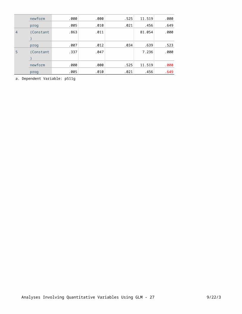
1 (Constant) .337 .047 7.236 .000

newform .000 .000 .525 11.519 .000

prog .005 .010 .021 .456 .649

2 (Constant) .340 .046 7.402 .000

newform .000 .000 .525 11.548 .000

3 (Constant) .337 .047 7.236 .000

newform .000 .000 .525 11.519 .000

prog .005 .010 .021 .456 .649

4 (Constant) .863 .011 81.054 .000

prog .007 .012 .034 .639 .523

5 (Constant) .337 .047 7.236 .000

newform .000 .000 .525 11.519 .000

prog .005 .010 .021 .456 .649


prog

newform

a. Dependent Variable: p511g


Key results –

1. There is no interaction of PROG and FORMULA. This can be interpreted as: “Formula is equally predictive for both programs.” or as “PROG difference is same at all ability levels.”

2. Controlling for FORMULA / Among persons equal on FORMULA, there is no significant difference in P511G performance between the two programs.

3. Controlling for Program / Among persons in the same program, there is a positive relationship of P511G to FORMULA.

Graphical representation of result:


1. Approximate parallelness of lines indicates nonsignificant PROD effect.

2. Approximate equal height of lines indicates nonsignificnt difference in Group means among persons equal on FORMULA.

3. Upward tilt of lines indicates significant relationship to FORMULA among persons in same Group.

Why did we have to use the stupid enter / remove /enter /remove sequence?

Any time that a research factor is represented by more than 1 variable, the enter / remove /enter sequence has to be used to insure that the error term is 1 – R2

All variables.

The first /enter puts ALL variables into the equation.

The remove takes just the variable or variables that are to be tested out.

Then the following enter adds the variables to be tested back into the equation, with the result being that the error term is 1 - R2

All variables because all variables are in the equation.

When do you NOT have to use the stupid enter / remove /enter sequence?

If EVERY research factor is represented by just one variable, then you can correctly assess the significance of each in just one model with all variables in the model.

That’s why the p-values of SPSS Model 7 above were exactly identical to the p-values associated with R2 change in the Model Summary Table – because in this particular example, all factors – prog, newform, and prog*newform – were one-variable factors.

So, any time each of your factors is represented by just one variable in a regression, you can simply put them all – main effects and interactions – into the equation and the tests will be appropriate.

But if even one factor needs two or more variables to represent it in regression, then I recommend using the enter / remove /enter sequence.


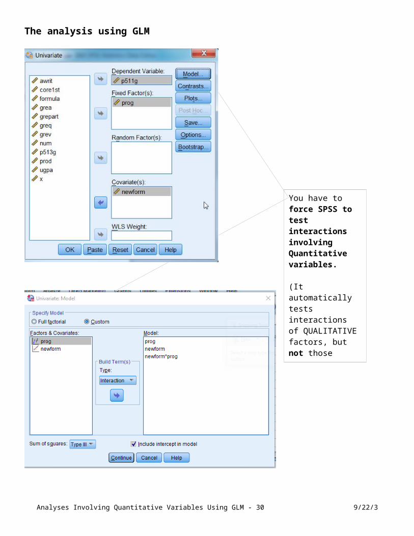
The analysis using GLM


You have to force SPSS to test interactions involving Quantitative variables.

(It automatically tests interactions of QUALITATIVE factors, but not those involving Quantitative variables.)


Estimated means are means, estimated assuming that all respondents have the same value for each covariate.

GET FILE='F:\MdbO\Dept\Validation\Valdat09.sav'.UNIANOVA p511g BY prog WITH newform /METHOD=SSTYPE(3) /INTERCEPT=INCLUDE /PLOT=PROFILE(prog) /EMMEANS=TABLES(prog) WITH(newform=MEAN) /PRINT=OPOWER ETASQ DESCRIPTIVE PARAMETER /CRITERIA=ALPHA(.05) /DESIGN=prog newform newform*prog.Univariate Analysis of Variance

Between-Subjects Factors

Value Label Nprog 0 RM 58

1 I/O 294

Descriptive StatisticsDependent Variable: p511gprog Mean Std. Deviation N0 RM .8630 .09211 581 I/O .8704 .07876 294Total .8692 .08101 352

Tests of Between-Subjects EffectsDependent Variable: p511g

SourceType III Sum of

Squares df Mean Square F Sig.Partial Eta Squared

Noncent. Parameter

Observed Powerb

Corrected Model .637a 3 .212 44.336 .000 .277 133.007 1.000Intercept .209 1 .209 43.544 .000 .111 43.544 1.000prog .001 1 .001 .128 .721 .000 .128 .065newform .541 1 .541 112.959 .000 .245 112.959 1.000prog * newform .000 1 .000 .099 .753 .000 .099 .061Error 1.667 348 .005Total 268.232 352Corrected Total 2.304 351


Parameter Estimates

Dependent Variable: p511g

Parameter B Std. Error t Sig.95% Confidence Interval Partial Eta

SquaredNoncent.

ParameterObserved

PowerbLower Bound Upper BoundIntercept .351 .055 6.386 .000 .243 .459 .105 6.386 1.000[prog=0] -.036 .101 -.358 .721 -.234 .162 .000 .358 .065[prog=1] 0a . . . . . . . .newform .000 4.637E-5 9.484 .000 .000 .001 .205 9.484 1.000[prog=0] * newform 2.682E-5 8.527E-5 .315 .753 .000 .000 .000 .315 .061[prog=1] * newform 0a . . . . . . . .a. This parameter is set to zero because it is redundant.


Estimated Marginal Means

progDependent Variable: p511g

prog Mean Std. Error95% Confidence Interval

Lower Bound Upper Bound0 RM .866a .009 .848 .8831 I/O .870a .004 .862 .878a. Covariates appearing in the model are evaluated at the following values: newform = 1180.54.


Struck through subcommands are default values.

We don’t have to follow the

Enter / remove /enter /remove sequence when using GLM because GLM automatically tests each effect with all other variables in the equation.

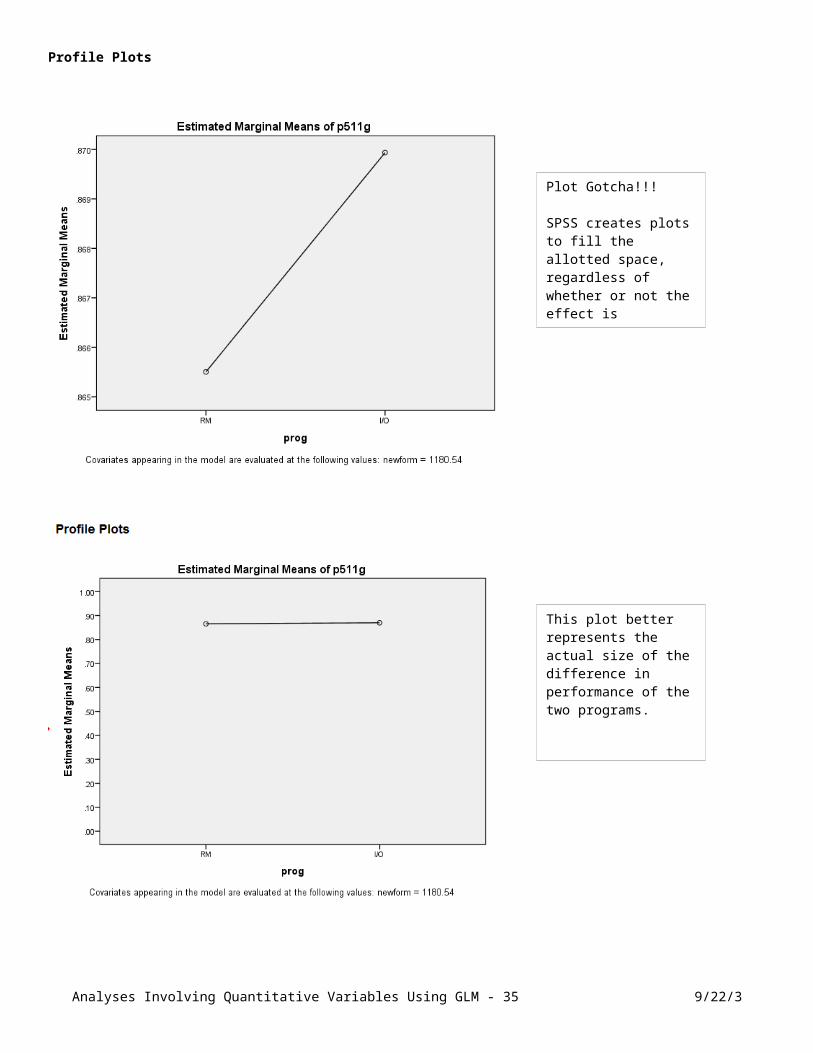
Profile Plots


Plot Gotcha!!!

SPSS creates plots to fill the allotted space, regardless of whether or not the effect is significant.

This plot better represents the actual size of the difference in performance of the two programs.

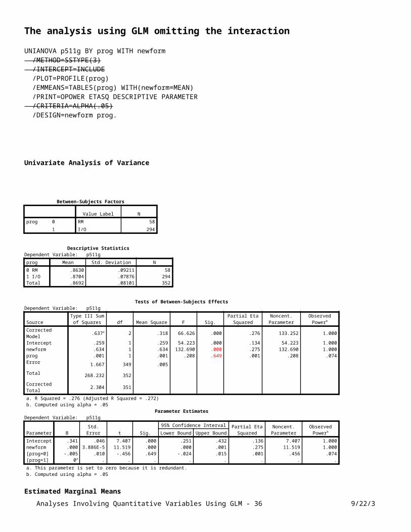
The analysis using GLM omitting the interactionUNIANOVA p511g BY prog WITH newform /METHOD=SSTYPE(3) /INTERCEPT=INCLUDE /PLOT=PROFILE(prog) /EMMEANS=TABLES(prog) WITH(newform=MEAN) /PRINT=OPOWER ETASQ DESCRIPTIVE PARAMETER /CRITERIA=ALPHA(.05) /DESIGN=newform prog.



Value Label Nprog 0 RM 58

1 I/O 294

Descriptive StatisticsDependent Variable: p511gprog Mean Std. Deviation N0 RM .8630 .09211 581 I/O .8704 .07876 294Total .8692 .08101 352

Tests of Between-Subjects EffectsDependent Variable: p511g

SourceType III Sum of

Squares df Mean Square F Sig.Partial Eta Squared

Noncent. Parameter

Observed Powerb

Corrected Model .637a 2 .318 66.626 .000 .276 133.252 1.000Intercept .259 1 .259 54.223 .000 .134 54.223 1.000newform .634 1 .634 132.690 .000 .275 132.690 1.000prog .001 1 .001 .208 .649 .001 .208 .074Error 1.667 349 .005Total 268.232 352Corrected Total 2.304 351


Parameter EstimatesDependent Variable: p511g

Parameter B Std. Error t Sig.95% Confidence Interval Partial Eta

SquaredNoncent.

ParameterObserved

PowerbLower Bound Upper BoundIntercept .341 .046 7.407 .000 .251 .432 .136 7.407 1.000newform .000 3.886E-5 11.519 .000 .000 .001 .275 11.519 1.000[prog=0] -.005 .010 -.456 .649 -.024 .015 .001 .456 .074[prog=1] 0a . . . . . . . .a. This parameter is set to zero because it is redundant.b. Computed using alpha = .05


progDependent Variable: p511g

prog Mean Std. Error95% Confidence Interval

Lower Bound Upper Bound0 RM .865a .009 .848 .8831 I/O .870a .004 .862 .878a. Covariates appearing in the model are evaluated at the following values: newform = 1180.54.


Profile Plots


Plot Gotcha!!!

SPSS creates plots to fill the allotted space, regardless of whether or not the effect is significant.

This plot better represents the actual size of the difference in performance of the two programs.

Example 2: Predicting GPA by Conscientiousness controlling for differences between experimental conditions. In Raven Worthy’s thesis, we assessed faking in three experimental conditions – 1: Honest condition - Participants were told to respond honestly.2: Instructed Faking condition – Participants were instructed to fake good to get a job.3: Incentives to Fake condition - Participants were given an incentive to fake.

We gave all participants the Big Five. About 1/3 of the participants were in each condition.

Our interest was on prediction of a criterion – GPA in this case – by conscientiousness, a quantitative factor.

So GPA was the dependent variable and Conscientiousness was the independent variable.Instructional Condition (Honest vs. Fake vs. Incentive) is a qualitative nuisance factor.

The interest here is on the relationship of GPA to conscientiousness.

We did not care about mean GPA differences between the three conditions, but since it was in the research design, we needed to control for any differences between groups that could cause variation in GPA that might obscure the relationships that we do care about – that of GPA to conscientiousness.

A more important issue associated with including the instructional condition groups in the analysis is whether the GPA to Conscientiousness relationship is the same from one group to another. This is an interaction question – Do Conscientiousness and Instructional Condition interact in the prediction of GPA?

So we include Instructional Condition as a factor in the analysis, mainly to determine whether or not the GPA to Conscientiousness relationship varies from one group to the next. If it does not, that means that Conscientiousness predicts GPA equally well regardless of the “mind set” of the respondents. If it does vary from one group to the next, that would mean that the validity of Conscientiousness depends on what the respondents are thinking when they take the personality test. That would be a problem for personality researchers.

This is essentially the opposite of a typical ANCOVA analysis. In a typical ANCOVA, we’re interested in mean differences between conditions and want to control for quantitative variables. Here, we’re interested in the relationships between two quantitative variables and want to control for differences between conditions.

Since cognitive ability is a predictor of GPA, we also controlled for it simply to increase power. This is a common “trick” that analysts use to increase the likelihood they’ll get significant results – controlling for factors that are unrelated to the predictors of interest, but related to the dependent variable. If they weren’t controlled for, the variance associated with differences in such variables would be in the denominator of the F statistic assessing significance of the predictors and would therefore reduce the value of F, making it less likely to be significant.

The complete analysis:

Regression of GPA onto Conscientiousness, Cognitive Ability, instructional condition and the interaction of Conscientiousness and Instructional Condition.

Thus we have 1) a continuous dependent variable, GPA, called eoygpa.2) a continuous research factor – Conscientiousness, called ContaminatedC here.3) a nominal research factor which we want to control for – Instructional Condition4) the interaction of ContaminatedC and Instructional Condition5) a continuous research factor which we want to control for – Cognitive Ability


Pre- analyses start here on 10/9/17.

Assessing the simple correlation of Contaminated C with GPA without controlling for anything.regression variables = eoygpa contaminatedC /dep=eoygpa /enter.[DataSet1] G:\MdbR\0DataFiles\Rosetta_CompleteData_110911.sav

Model Summary

Model R R SquareAdjusted R Square

Std. Error of the Estimate

1 .163a .027 .024 .6387a. Predictors: (Constant), contaminatedC

Coefficientsa



t Sig.B Std. Error Beta1 (Constant) 2.440 .178 13.683 .000

contaminatedC .100 .034 .163 2.981 .003a. Dependent Variable: EOYGPAThe relationship is significant, but r is only .163. It could be that r is suppressed by irrelevant variance due to faking.

The Analyses using REGRESSIONBasic Analysis with interaction– GPA regressed onto ContaminatedC, Instructional Condition, Cognitive Ability, and ContaminatedC * Instructional Condition – focusing on the interaction.

There were 3 groups, so two group-coding variables were required to represent them. The group codes were . . .

DCF: A contrast code comparing the honest condition vs the two faking conditions (1 vs 2&3), andDCI: A contrast code comparing Incentive faking with Instructed Faking (2 vs 3), with honest condition group set to 0.compute CxDCF = contaminatedC * DCF.compute CxDCI = contaminatedC * DCI.

Here an overview of the data.

Instructional CognitiveCondition GPA C DCF DCI CxDCF CxDCI AbilityHonest GPA C .667 0 C*.667 C*0 wptFake GPA C -.333 .5 C*-.333 C*.5 wptIncentive GPA C -.333 -.5 C*-.333 C*-.5 wpt

The Cognitive Ability variable is called wpt because the Wonderlic Personnel Test was used as the measure of cognitive ability.

I’m not sure why we used the names DCF and DCI. F and I stand for Faking and Incentive. I don’t remember what the DC is supposed to represent. It should be CC, for Contrast Codes, but no time to change all of the screen shots..


I computed interaction terms as products of the main effects.

Using the REGRESSION procedure to assess the significance of the interaction of Conscientiousness and Instructional Condition.

regression variables = eoygpa contaminatedC wpt dcf dci CxDCF CxDCI /sta=default cha/dep=eoygpa /enter/remove CxDCF CxDCI /enter CxDCF CxDCI.

Model Summary

Model RR

SquareAdjusted R

SquareStd. Error of the Estimate

Change StatisticsR Square Change

F Change df1 df2

Sig. F Change

1 .381a .145 .129 .6032 .145 9.084 6 321 .0002 .379b .144 .133 .6019 -.002 .301 2 321 .7403 .381c .145 .129 .6032 .002 .301 2 321 .740 a. Predictors: (Constant), CxDCI, dcF, wpt, contaminatedC, CxDCF, dcIb. Predictors: (Constant), dcF, wpt, contaminatedC, dcIc. Predictors: (Constant), dcF, wpt, contaminatedC, dcI, CxDCF, CxDCI

The interaction of ContaminatedC with Instructional Conditions was not significant. So the relationship of GPA to contaminatedC was the same across all three conditions.

Dropping the interaction term – focusing on the Conscientiousness -> GPA relationship

Does Conscientioiusness predict GPA when controlling for both Instructional Condition and Cognitive Ability?

This is a simple, simultaneous regression with all predictors entered at once.

Model Summary

Model R R Square

Adjusted R

Square

Std. Error of the

Estimate

1 .379a .144 .133 .6019

a. Predictors: (Constant), dcI, dcF, wpt, contaminatedC

Coefficientsa

Model

Unstandardized Coefficients

Standardized

Coefficients

t Sig.B Std. Error Beta

1 (Constant) 1.564 .216 7.247 .000

contaminatedC .117 .034 .190 3.475 .001

wpt .036 .006 .293 5.612 .000

dcF -.254 .073 -.185 -3.479 .001

dcI .148 .084 .093 1.762 .079

a. Dependent Variable: EOYGPA

The significant t value for ContaminatedC tells us that when controlling for both Instructional Condition and Cognitive ability, GPA is related to ContaminatedC. So this measure of Conscientiousness is robust with respect to the “mind set” of respondents and also with respect to the cognitive ability of the respondents.

Note that the significant dcF t value tells us that there was a significant difference in mean GPA between the honest and the two faking conditions. Since the assignment to conditions was made randomly, we attribute this difference to chance.


The analysis using GLM


I checked the Parameter Estimates box in the above dialog box, but I do not show it below in the interests of continuity and space.

UNIANOVA EOYGPA BY ncondit WITH contaminatedC wpt /METHOD=SSTYPE(3) /INTERCEPT=INCLUDE /PRINT ETASQ DESCRIPTIVE PARAMETER OPOWER /CRITERIA=ALPHA(.05) /DESIGN=ncondit contaminatedC contaminatedC*ncondit wpt.Univariate Analysis of VarianceBetween-Subjects Factors

N

ncondit 1 110

2 108

3 110

Descriptive StatisticsDependent Variable: EOYGPA

ncondit Mean Std. Deviation N

1 3.077 .5581 110

2 2.891 .7318 108

3 2.915 .6289 110

Total 2.962 .6464 328


Tests of Between-Subjects EffectsDependent Variable: EOYGPA

Source

Type III Sum of

Squares dfMean

Square F Sig.Partial Eta Squared

Noncent. Parameter

Observed Powerb

Corrected Model 19.829a 6 3.305 9.084 .000 .145 54.504 1.000Intercept 19.009 1 19.009 52.249 .000 .140 52.249 1.000ncondit .250 2 .125 .344 .709 .002 .688 .105contaminatedC 4.214 1 4.214 11.582 .001 .035 11.582 .924ncondit * contaminatedC

.219 2 .110 .301 .740 .002 .602 .098

wpt 11.436 1 11.436 31.435 .000 .089 31.435 1.000Error 116.783 321 .364

Total 3013.419 328



So the interaction term is not significant with the same p-value as we got using REGRESSION.

Some analysts would interpret the significant of ContaminatedC from the above table, which controls for the interacton.

Others would rerun the analysis, leaving out the interaction test, assessing the significance of ContaminatedC controlling for ncondit and wpt, but not controlling for the interaction.

The reason we would drop the interaction is because interaction terms are quite often highly correlated with the main effects.

If A and B are main effect, the interaction is A*B. Alas, A*B is correlated with A and also with B.

So, including the interaction includes a highly correlated variable as a controlling variable in the analysis. Since it’s not significant (we’ve already assessed that), it’s “stealing” variance in the dependent variable from A and also from B. Including it might make them not significant because recall that significance in a multiple regression is increase in R-square over and above the other variables.

For this reason, I’d say that the majority of analysts would drop a nonsignificant interaction.

Note that the GLM analysis did not give us the contrasts DCF and DCI that we got from REGRESSION.

It is possible to create contrasts using syntax in GLM, but it is quite time consuming unless you’re facile with syntax.


The analysis with GLM not including the interaction

Tests of Between-Subjects EffectsDependent Variable: EOYGPA

Source

Type III Sum of

Squares dfMean

Square F Sig.Partial Eta Squared

Noncent. Parameter

Observed Powerb

Corrected Model

19.610a 4 4.902 13.534 .000 .144 54.136 1.000

Intercept 19.025 1 19.025 52.520 .000 .140 52.520 1.000ncondit 5.265 2 2.633 7.268 .001 .043 14.535 .935contaminatedC 4.375 1 4.375 12.078 .001 .036 12.078 .934wpt 11.407 1 11.407 31.489 .000 .089 31.489 1.000Error 117.002 323 .362

Total 3013.419 328

Corrected Total

136.612 327


The good news for our sanity is that the significance of ContaminatedC does not change when the nonsignifica nt interation was dropped. So our conclusion that C predicts GPA controlling for instructonal condition and wpt is a robust one, that holds up whether or not the interaction is in the equation.


Example 3. Energy Usage predicted by Two Qualitative Factors and One Quantitative Variable

Factorial Analysis of CovarianceFrom Howell, p. 610. The data represent two factors - interest in a program to reduce electric bills.

GROUP: Group 1 enrolled in a program. Group 2 showed interest, but didn’t enroll. Group 3 showed no interest.

METER: Half the participants had a meter installed that showed daily electric power usage. The other half did not.

So GROUP and METER form a 3x2 factorial design.

COV: The quant factor was last year’s bill.

_

Y COV GROUP METER G1 G2 M G1xM G2xM G1xV G2xV MxV G1xMxV G2xMxV

58 75 1 0 .33 .50 -.50 -.17 -.25 24.75 37.50 -37.50 -12.38 -18.75 25 40 1 0 .33 .50 -.50 -.17 -.25 13.20 20.00 -20.00 -6.60 -10.00 50 68 1 0 .33 .50 -.50 -.17 -.25 22.44 34.00 -34.00 -11.22 -17.00 40 62 1 0 .33 .50 -.50 -.17 -.25 20.46 31.00 -31.00 -10.23 -15.50 55 67 1 0 .33 .50 -.50 -.17 -.25 22.11 33.50 -33.50 -11.06 -16.75 25 42 1 1 .33 .50 .50 .17 .25 13.86 21.00 21.00 6.93 10.50 38 64 1 1 .33 .50 .50 .17 .25 21.12 32.00 32.00 10.56 16.00 46 70 1 1 .33 .50 .50 .17 .25 23.10 35.00 35.00 11.55 17.50 50 67 1 1 .33 .50 .50 .17 .25 22.11 33.50 33.50 11.06 16.75 55 75 1 1 .33 .50 .50 .17 .25 24.75 37.50 37.50 12.38 18.75 60 70 2 0 .33 -.50 -.50 -.17 .25 23.10 -35.00 -35.00 -11.55 17.50 30 25 2 0 .33 -.50 -.50 -.17 .25 8.25 -12.50 -12.50 -4.13 6.25 55 65 2 0 .33 -.50 -.50 -.17 .25 21.45 -32.50 -32.50 -10.73 16.25 50 50 2 0 .33 -.50 -.50 -.17 .25 16.50 -25.00 -25.00 -8.25 12.50 45 55 2 0 .33 -.50 -.50 -.17 .25 18.15 -27.50 -27.50 -9.08 13.75 40 55 2 1 .33 -.50 .50 .17 -.25 18.15 -27.50 27.50 9.08 -13.75 47 52 2 1 .33 -.50 .50 .17 -.25 17.16 -26.00 26.00 8.58 -13.00 56 68 2 1 .33 -.50 .50 .17 -.25 22.44 -34.00 34.00 11.22 -17.00 28 30 2 1 .33 -.50 .50 .17 -.25 9.90 -15.00 15.00 4.95 -7.50 55 72 2 1 .33 -.50 .50 .17 -.25 23.76 -36.00 36.00 11.88 -18.00 75 80 3 0 -.67 .00 -.50 .34 .00 -53.60 .00 -40.00 26.80 .00 60 55 3 0 -.67 .00 -.50 .34 .00 -36.85 .00 -27.50 18.43 .00 70 73 3 0 -.67 .00 -.50 .34 .00 -48.91 .00 -36.50 24.46 .00 65 61 3 0 -.67 .00 -.50 .34 .00 -40.87 .00 -30.50 20.44 .00 55 65 3 0 -.67 .00 -.50 .34 .00 -43.55 .00 -32.50 21.78 .00 55 56 3 1 -.67 .00 .50 -.34 .00 -37.52 .00 28.00 -18.76 .00 62 74 3 1 -.67 .00 .50 -.34 .00 -49.58 .00 37.00 -24.79 .00 57 60 3 1 -.67 .00 .50 -.34 .00 -40.20 .00 30.00 -20.10 .00 50 68 3 1 -.67 .00 .50 -.34 .00 -45.56 .00 34.00 -22.78 .00 70 76 3 1 -.67 .00 .50 -.34 .00 -50.92 .00 38.00 -25.46 .00

The contrasts that would be required if we were to do the analysis using REGRESSION are shown above.The analysis could be conducted using REGRESSION, but I’ll illustrate the analysis using GLM below.

Group Contrast 1: Is the mean of Groups with any interest equal to mean of Group with no interest?Group Contrast 2: Is the mean of Group enrolled equal to mean of Group which just showed interest?

G1 x Meter: Is the difference between Groups with any interest and Group with no interest related to whether or not participants had a meter?G2 x Meter: Is the difference between Enrollees and those just showing interest related to whether or not participants had a meter?


GROUP x METERInteractionContrasts

MeterContrasts

GROUPContrasts

GROUP x COV

InteractionContrasts

METER x COV

InteractionContrasts

GROUP x METER x

COVInteractionContrasts

Part A: Analysis using GLM, with Interactions involving the Covariate

comment With covariate interactions.UNIANOVA y BY group meter WITH cov /METHOD = SSTYPE(3) /INTERCEPT = INCLUDE /CRITERIA = ALPHA(.05) /DESIGN = group meter cov group*meter cov*group cov*meter cov*group*meter .



Whew! The interactions are not significant. We don’t have to interpret them.

Getting the covariate interactions via. Dialog boxes.

Test s of Bet w een- Subj ect s Ef f ect s

Dependent Var iable: Y

4364. 926a 11 396. 811 16. 542 . 000

36. 555 1 36. 555 1. 524 . 233

188. 435 2 94. 217 3. 928 . 038

1. 080 1 1. 080 . 045 . 834

1766. 037 1 1766. 037 73. 623 . 000

3. 883 2 1. 942 . 081 . 923

75. 666 2 37. 833 1. 577 . 234

1. 175 1 1. 175 . 049 . 827

3. 794 2 1. 897 . 079 . 924

431. 774 18 23. 987

82521. 000 30

4796. 700 29

Sour ceCor r ect ed M odel

I nt er cept

G RO UP

M ETER

CO V

G RO UP * M ETER

G RO UP * CO V

M ETER * CO V

G RO UP * M ETER *CO V

Er r or

Tot al

Cor r ect ed Tot al

Type I I I Sumof Squar es df M ean Squar e F Sig.

R Squar ed = . 910 ( Adjust ed R Squar ed = . 855)a.

Part B: Analysis using GLM using GLM’s default approach with no interactions involving the covariate (since they were all NS).comment Without covariate interactions.UNIANOVA y BY group meter WITH cov /METHOD = SSTYPE(3) /INTERCEPT = INCLUDE /PLOT = PROFILE( group*meter ) /EMMEANS = TABLES(group) WITH(cov=MEAN) /EMMEANS = TABLES(meter) WITH(cov=MEAN) /EMMEANS = TABLES(group*meter) WITH(cov=MEAN) /PRINT = DESCRIPTIVE ETASQ OPOWER HOMOGENEITY /CRITERIA = ALPHA(.05) /DESIGN = cov group meter group*meter .




10

10

10

15

15

1.00

2.00

3.00

GROUP

.00

1.00

METER

N

De s c riptiv e Sta tis tic s

De p e n d e n t Va ria b l e : Y

4 5 .6 0 0 0 1 3 .3 9 0 2 9 5

4 2 .8 0 0 0 11 .7 3 4 5 6 5

4 4 .2 0 0 0 11 .9 6 1 0 5 1 0

4 8 .0 0 0 0 11 .5 1 0 8 6 5

4 5 .2 0 0 0 11 .6 0 6 0 3 5

4 6 .6 0 0 0 1 0 .9 9 6 9 7 1 0

6 5 .0 0 0 0 7 .9 0 5 6 9 5

5 8 .8 0 0 0 7 .5 9 6 0 5 5

6 1 .9 0 0 0 8 .0 0 6 2 5 1 0

5 2 .8 6 6 7 1 3 .6 6 8 8 7 1 5

4 8 .9 3 3 3 1 2 .1 4 4 7 6 1 5

5 0 .9 0 0 0 1 2 .8 6 0 9 3 3 0

METER.0 0

1 .0 0

To ta l

.0 0

1 .0 0

To ta l

.0 0

1 .0 0

To ta l

.0 0

1 .0 0

To ta l

GROUP1 .0 0

2 .0 0

3 .0 0

To ta l

Me a n Std . De v ia ti o n N

L e v e n e ' s T e s t o f Eq u a l i ty o f Erro r Va ria n c e sa

De p e n d e n t Va ri a b l e : Y

.4 9 1 5 2 4 .7 8 0F d f1 d f2 S i g .

T e s ts th e n u l l h y p o th e s i s th a t th e e rro r v a ri a n c e o f th e d e p e n d e n tv a ri a b l e i s e q u a l a c ro s s g ro u p s .

De s i g n : In te rc e p t+ COV+ GROUP+ MET ER+ GROUP * MET ERa .

The default GLM analysis



Te s ts o f Be twe e n-Subje c ts Effe c ts

De p e n d e n t Va ria b le : Y

4 2 8 3 .9 0 1 b 6 7 1 3 .9 8 3 3 2 .0 2 3 .0 0 0 .8 9 3 1 9 2 .1 4 1 1 .0 0 0

4 5 .4 6 9 1 4 5 .4 6 9 2 .0 3 9 .1 6 7 .0 8 1 2 .0 3 9 .2 7 8

2 3 0 4 .8 0 1 1 2 3 0 4 .8 0 1 1 0 3 .3 7 5 .0 0 0 .8 1 8 1 0 3 .3 7 5 1 .0 0 0

11 2 0 .8 7 2 2 5 6 0 .4 3 6 2 5 .1 3 7 .0 0 0 .6 8 6 5 0 .2 7 3 1 .0 0 0

1 7 2 .6 9 7 1 1 7 2 .6 9 7 7 .7 4 6 .0 11 .2 5 2 7 .7 4 6 .7 6 0

8 .2 4 6 2 4 .1 2 3 .1 8 5 .8 3 2 .0 1 6 .3 7 0 .0 7 5

5 1 2 .7 9 9 2 3 2 2 .2 9 6

8 2 5 2 1 .0 0 0 3 0

4 7 9 6 .7 0 0 2 9

So u rc eCo rre c te d Mo d e l

In te rc e p t

COV

GROUP

METER

GROUP *METER

Erro r

To ta l

Co rre c te d T o ta l

Ty p e III Su mo f Sq u a re s d f Me a n Sq u a re F Sig .

Pa rtia l EtaSq u a re d

No n c e n t.Pa ra me te r Ob s e rv e d Po we r

a

Co mp u te d u s in g a lp h a = .0 5a .

R Sq u a re d = .8 9 3 (Ad ju s te d R Sq u a re d = .8 6 5 )b .

1. GROUP

Dependent Variable: Y

42.990a 1. 498 39.891 46.089

51.779a 1. 578 48.515 55.042

57.931a 1. 543 54.739 61.124

GROUP1. 00

2. 00

3. 00

Mean St d. Error Lower Bound Upper Bound

95% Conf idence Interval

Evaluat ed at covariat es appeared in t he model: COV = 61.3333.a.

2. METER


53.302a 1. 220 50.779 55.826

48.498a 1. 220 45.974 51.021

METER.00

1. 00


95% Conf idence Interval

Evaluat ed at covariat es appeared in t he model: COV = 61.3333.a.

3. GROUP * METER


44. 826a 2. 113 40. 454 49. 197

41. 154a 2. 118 36. 773 45. 536

54. 050a 2. 194 49. 511 58. 588

49. 507a 2. 154 45. 052 53. 963

61. 031a 2. 147 56. 589 65. 474

54. 831a 2. 147 50. 389 59. 274

METER. 00

1. 00

. 00

1. 00

. 00

1. 00

GROUP1. 00

2. 00

3. 00


95% Conf idence I nt erval

Evaluat ed at covar iat es appeared in t he model: COV = 61. 3333.a.

Profile Plots

This shows that estimated means can be quite different from observed means.

The observed means, put there by me, are what they are – the actual means that we observed.

The expected means are what the means would have been had everyone used the same amount of power in the previous year – the covariate.

GLM automatically plots the expected means.


Nonmetered Observed mean

Metered Observed mean

Estimated Marginal Means of Y

GROUP

Showed no int erest iI nquired, but didn'tEnrolled in program

Es

tim

ate

d M

arg

ina

l M

ea

ns

70

60

50

40

METER

Nonmet ered

Met ered

Issues

1. Control – What other variables should be controlled for when assessing the main effect of a research factor or the interaction of two research factors?

General solution: For each variable, control for all other variables and all significant interactions of the variable with other variables.

Controlling for all means you’re assessing the unique relationship of the dependent variable to the variable of interest.

2. The error term.

Use as the error term 1 – R2All IV’s’s including interactions.

You have to check to make sure that all IVs are in the error term. This may require manual computations.

The error term represents variation in the dependent variable that you are unable to account for. So it’s random error. It is the standard against which all tests of significance are based.

So, if you’re hoping for “significance,” you should make the error term as small as possible. That will insure that you will be able to detect even small amounts of variation due to the variable of interest.

3. Interactions – What interactions should be created and tested for?

GLM automatically creates and tests for (and controls for) all interactions between qualitative research factors. It must be told to exclude interactions, if that’s what you want.

GLM does NOT create or test for interactions involving quantitative research factors. It must be forced to create them. Once they’re created, it can test for them.

This is unfortunate, because even in the simplest type of analysis involving qualitative and quantitative factors, perhaps especially in the simplest type, the test of the interaction of the qualitative research factor with the quantitative, called the test of equality of slopes, is an important test.

However, since it is common practice to NOT control for qualitative x quantitative interactions when testing significance of qualitative research factors, I believe that GLM’s rule is close to existing practice.


Analyses using GLM - The University of Tennessee at ... · Web viewAnalyses Involving Only...

Documents

Transcript of Analyses using GLM - The University of Tennessee at ... · Web viewAnalyses Involving Only...