An individual-based model for black bears in the

southern Appalachians

Rene A. Salinasa,∗, Louis J. Grossb, Frank T. van Manenc, Joseph D. Clarkc

aDepartment of Mathematical Sciences, Appalachian State University, Boone, North

Carolina 28608, USAbNational Institute for Mathematical and Biological Synthesis, University of Tennessee,

Knoxville, Tennessee 37996-1527, USAcUSGS Southern Appalachian Research Branch, University of Tennessee, Knoxville,

Tennessee 37901-1071, USA

Abstract

We describe an individual-based model for black bears (Ursus americanus)

in the southern Appalachians, which consists of Great Smoky Mountains

National Park (GSMNP), Cherokee (CNF), Pisgah (PNF), and Nantahala

(NNF) national forests, and most of eastern Tennessee and western North

Carolina. This model incorporates fall hard mast variation which determines

black bear reproductive success and movement. We evaluated the model with

existing empirical data on harvest, year-to-year variation, and reproductive

dynamics. To demonstrate the potential use of the model for spatial control,

we tested an alternative harvesting strategy in a subregion of the model to

address concerns regarding potential bear-human encounters. This model

has the capability to provide insight into the hard mast-driven dynamics of

the back bear population and test the effectiveness of different harvesting

∗Corresponding AuthorEmail addresses: salinasra@appstate.edu (Rene A. Salinas)URL: mathsci2.appstate.edu/∼ras (Rene A. Salinas)

Preprint submitted to Ecological Modelling December 8, 2011

strategies.

Key words: Individual-based, Black bear, Hard mast, Spatial control,

Harvest management, Bear-human encounters

1. Introduction

The establishment of Great Smoky Mountains National Park (GSMNP)

in the mid-1930s created a protected environment for many over-exploited

species. One of the species that benefited was the black bear (Ursus ameri-

canus), which became a source population for the surrounding region. GSMNP

is surrounded by numerous small tourist towns and sprawling suburban areas.

and the human population surrounding GSMNP has been increasing, partic-

ularly during the last three decades. This change in human population and

increase in the black bear population has led to an increase in bear-human

encounters and nuisance incidents (Delozier and Stiver, 2005).

There are two principal reasons bears leave GSMNP and other protected

regions: to establish a home range and search for food. During summer,

sub-adult bears leave their mothers and find areas where they can establish

home ranges. Female offspring usually establish home ranges near those of

their mother, whereas male offspring disperse further (Rogers, 1987; Costello,

2010). During the fall, bears may move greater distances searching for food

to build up fat reserves for hibernation (Quigley, 1982; Carr, 1983; Rogers,

1987). Their primary fall food source in the southern Appalachians is hard

mast, principally acorns (Beeman and Pelton, 1970; Eagle and Pelton, 1981;

Brody and Pelton, 1988), which can vary from year to year. During years

of hard mast failure, bears may move out of protected areas in search of

2

food. Variation in hard mast also affects female reproductive success. If a

female is unable to gain sufficient weight, lactation may be insufficient to

feed her litter, resulting in cub mortality during the denning period (Eiler

et al., 1989).

Bear conflicts are not unique to the southern Appalachians. Throughout

the range of the species, the successful recovery of black bear populations,

coupled with urban sprawl, has resulted in increased nuisance activity (Tim-

mins, 2005; Dente and Renar, 2005; Martin and Steffen, 2005; Ryan, 2005).

The importance of public opinion on wildlife management practices is well

documented (Decker and Chase, 1997), particularly if the public perceives a

species as dangerous, and they may be less and management agencies may

be less willing to promote conservation issues related to a particular species

if the public perceives it as dangerous. One option wildlife managers have is

to control wildlife populations through sport hunting, thereby reducing the

populations and the potential for harmful interactions. However, information

on optimal harvest strategies to carry out such controls is lacking.

Models are a powerful tool in the development of management strategies

(Miller, 1992; Schoen, 1992; McCullough, 1996). Most of the models that

have addressed black bear management have been deterministic Leslie-type

models accounting for demographics (Yodzis and Kolenosky, 1986; Burton

et al., 1994; McCullough, 1996). Such models are not able to address space

explicitly and are therefore limited in their management implications. Wie-

gand et al. (1998) developed a spatially explicit simulation model to deter-

mine the risk of extinction of brown bears (Ursus arctos) in Spain. However,

this model did not include intra-year dynamics of the bear population, which

3

is vital to assess management strategies.

Understanding the year-to-year dynamics of black bears, or any species

targeted for management, is vital to developing an effective harvesting strat-

egy. Harvest management, composed of effort, location, and time, is a spatial

control problem. Each of the components of harvesting can affect the pop-

ulation in different ways. Therefore, a model must have enough detail to

account for these effects. We address this issue by developing a spatially-

explicit individual-based model (IBM) for black bears in the southern Ap-

palachian region. IBMs involve modeling the life stages of each individual

via a set of rules based on life history data of the organism (DeAngelis and

Gross, 1992; Grimm and Railsback, 2005). To demonstrate the potential of

the model, we explore the effects of fall hard mast on population dynamics

and the effects of allowing hunting in a state-designated bear sanctuary on

black bear abundance and potential bear-human interactions.

2. Model Description

This section follows the protocol for describing IBMs proposed by Grimm

at al (2006).

2.1. Purpose

The main purpose of the model is to provide managers with a tool appli-

cable for assessment of management activity impacts on the dynamics of the

black bear population in the southern Appalachians. The model allows many

facets of the population to be studied. This paper focuses on the description

of the model, its evaluation, and an example of how the model can be used

4

as a tool for spatial control of harvesting to minimize potential bear-human

encounters.

2.2. State Variables and Scale

State variables for the model can be divided into two groups: those for

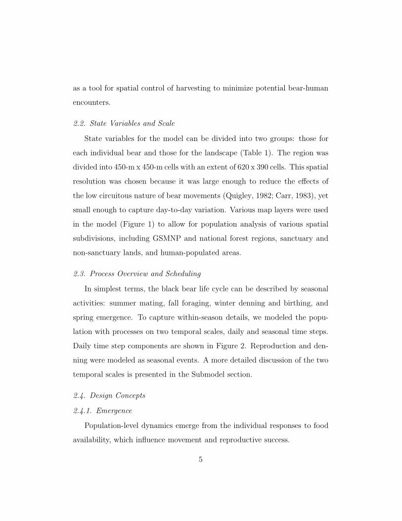
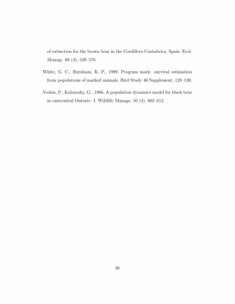
each individual bear and those for the landscape (Table 1). The region was

divided into 450-m x 450-m cells with an extent of 620 x 390 cells. This spatial

resolution was chosen because it was large enough to reduce the effects of

the low circuitous nature of bear movements (Quigley, 1982; Carr, 1983), yet

small enough to capture day-to-day variation. Various map layers were used

in the model (Figure 1) to allow for population analysis of various spatial

subdivisions, including GSMNP and national forest regions, sanctuary and

non-sanctuary lands, and human-populated areas.

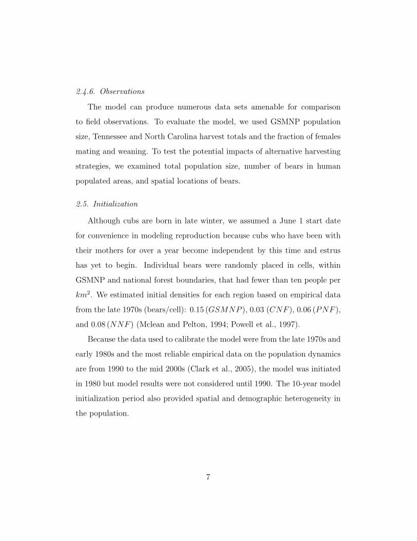
2.3. Process Overview and Scheduling

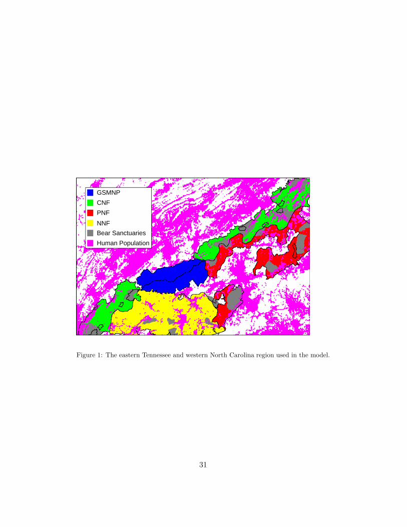
In simplest terms, the black bear life cycle can be described by seasonal

activities: summer mating, fall foraging, winter denning and birthing, and

spring emergence. To capture within-season details, we modeled the popu-

lation with processes on two temporal scales, daily and seasonal time steps.

Daily time step components are shown in Figure 2. Reproduction and den-

ning were modeled as seasonal events. A more detailed discussion of the two

temporal scales is presented in the Submodel section.

2.4. Design Concepts

2.4.1. Emergence

Population-level dynamics emerge from the individual responses to food

availability, which influence movement and reproductive success.

5

2.4.2. Adaptation

The model assumes bears adapt their movements based on two factors:

food availability and proximity to older bears. These factors are described

in detail in the movement submodel.

2.4.3. Sensing

Individual bears can sense the amount of food available around them up

to their maximum daily movement range. They also are aware of other bears

in the vicinity (see Submodel section).

2.4.4. Interaction

Two forms of direct interaction between individuals are included in the

model. Mating occurs during the summer and is determined by males finding

nearest females that are in estrus. Bear movement is partially determined

by interaction tolerances in which younger bears are less likely to go to a cell

with older bears. These tolerances are differentiated by sex and described in

detail in the movement submodel.

2.4.5. Stochasticity

All daily and seasonal event probabilities occur based on comparisons us-

ing a pseudorandom number generator. The inherent variation in the model

was assessed for each scenario through 20 iterations of the model with differ-

ent seeds for the pseudorandom number generator. The number of iterations

was chosen based on a comparison of the 95% CI for population size in

GSMNP which showed significant diminishing returns after 20 iterations.

6

2.4.6. Observations

The model can produce numerous data sets amenable for comparison

to field observations. To evaluate the model, we used GSMNP population

size, Tennessee and North Carolina harvest totals and the fraction of females

mating and weaning. To test the potential impacts of alternative harvesting

strategies, we examined total population size, number of bears in human

populated areas, and spatial locations of bears.

2.5. Initialization

Although cubs are born in late winter, we assumed a June 1 start date

for convenience in modeling reproduction because cubs who have been with

their mothers for over a year become independent by this time and estrus

has yet to begin. Individual bears were randomly placed in cells, within

GSMNP and national forest boundaries, that had fewer than ten people per

km2. We estimated initial densities for each region based on empirical data

from the late 1970s (bears/cell): 0.15 (GSMNP ), 0.03 (CNF ), 0.06 (PNF ),

and 0.08 (NNF ) (Mclean and Pelton, 1994; Powell et al., 1997).

Because the data used to calibrate the model were from the late 1970s and

early 1980s and the most reliable empirical data on the population dynamics

are from 1990 to the mid 2000s (Clark et al., 2005), the model was initiated

in 1980 but model results were not considered until 1990. The 10-year model

initialization period also provided spatial and demographic heterogeneity in

the population.

7

2.6. Submodels

2.6.1. Mast Layer

In the southern Appalachians, soft and hard mast are black bears’ prin-

cipal food sources for most of the year (Beeman and Pelton, 1970; Brody

and Pelton, 1988; Eagle and Pelton, 1981). Soft mast, which includes berries

and other fleshy fruits, provides most nutrition during summer. Hard mast,

which includes acorns and other dry fruits, provides vital nutrition during the

fall. Bears use hard mast to gain fat reserves for the winter denning period.

Fall hard mast failures occur, on average, every four to five years (Koenig

and Knops, 2000). It has been hypothesized that years of above average soft

mast abundance can compensate for hard mast failures (Inman and Pelton,

2002). There were no data on the variability of soft mast in the region, so a

constant soft mast availability was assumed.

Hard mast availability was simulated using a vegetation map layer that

included nine forest types and one non-forest type (urban). Kilocalories

(kcal) of available food throughout the year were estimated for each vegeta-

tion class using data derived for the northwestern section of GSMNP in 1995

(Inman and Pelton, 2002). The available kilocalories were updated every 2

weeks throughout the year. Because 1995 was an average fall mast year (In-

man and Pelton, 2002), the data were scaled to approximate maximum mast

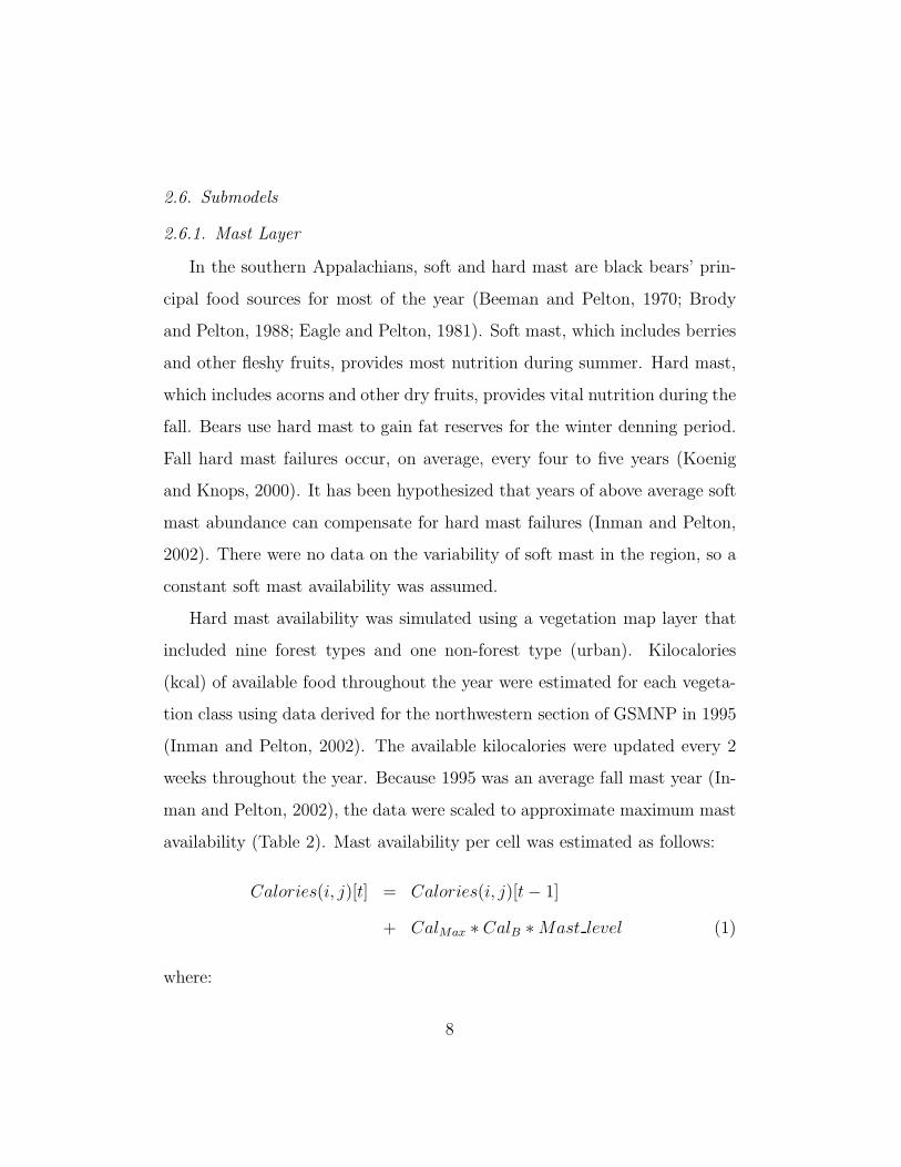
availability (Table 2). Mast availability per cell was estimated as follows:

Calories(i, j)[t] = Calories(i, j)[t − 1]

+ CalMax ∗ CalB ∗ Mast level (1)

where:

8

• i, j designate the coordinates of the cell.

• CalMax = Caloriesveg type[montht]/2, represents the number of kilo-

calories of the vegetation type in cell(i,j) for the month of time t. It is

divided by 2 because mast is replaced every 14 days in the model.

• CalB is the proportion of the kilocalories available to bears. Between

70 - 90% of mast is used by birds and small mammals (Darley-Hill

and Johnson, 1981; Steiner, 1996; Inman and Pelton, 2002). For the

summer, we assume 30% is available, whereas only 10% is assumed to

be available during the fall.

• Mast level =(

Mastyear(t) + randomunif

)

/10 represents the mast in-

dex value for that year. Mastyear(t) ranges from 1 - 4. An index value of

1.0 represents a failure and 4.0 represents maximum mast production.

Because no data were available on soft mast variation during summer,

we assumed Mastyear(t) = 3. During a given masting event, not all

trees produce the same amount of mast (Greenberg, 2000). Therefore,

to allow for spatial variability, the actual index value in each cell is uni-

formly distributed between [Index − 0.5, Index + 0.5]. The number is

then divided by 10 to represent the value as a proportion. For the data

we represent in this paper, the following years were considered mast

failure in GSMNP: 1992, 1997, and 2003.

Equation 1 does not represent the actual number of kilocalories in each cell.

Instead, it is a metric of available food.

9

2.6.2. Movement

Bears have a hierarchical dominance structure in which older, larger males

acquire home ranges that include the best food resources (Rogers, 1987; Pow-

ell, 1987). Older females have a similar advantage over younger females.

Movement was modeled solely based on food availability and this hierarchi-

cal dominance structure. The model assumed bears move to cells with the

most food. There are three components to bear movement: dominance, daily

range, and seasonal territories.

Dominance was defined by age and differentiated by sex. A male could

move into a cell if there were no older males within a one-cell radius, whereas

females (and their cubs) could enter a cell if there were no older females in

that cell (0-cell radius). The difference in this “tolerance” spacing between

males (1-cell radius) and females (0-cell radius) is supported by data suggest-

ing that females are more tolerant than males and often share home ranges

with offspring (Quigley, 1982; Carr, 1983).

Each bear searched outwardly from its current cell. Males could move as

far as four cells in one day, whereas females were limited to two (Quigley,

1982; Carr, 1983). If a bear was unable to find a suitable cell, it was randomly

placed in one of the cells in its outer daily movement range. Because the

cells are 450 m x 450 m, more than one bear can occupy the same cell.

The movement rules allow for this because older bears can move to any cell

despite the number of younger bears in it.

There are two seasonal movement patterns for black bears: Summer mat-

ing and Fall foraging. During the mating season, if a female is in estrus, the

nearest adult male is moved to her cell to copulate. Once copulation occurs,

10

both male and female move to find food according to the above rules.

On June 1st and September 1st, positions of each sub-adult and adult are

saved as a central location. As a bear moves closer to its maximum distance

(eight cells for males, five for females) from this central location, the search

region is skewed away from the maximum distance. For example, if a male is

six cells east of its center, its search region in the x-direction was restricted

to two cells to the east and four cells to the west (recall that males have

a maximum search range of eight cells.). This implemented a restriction

in uni-directional movement. When a bear reaches a cell at its maximum

distance, the central location is reset to that point to allow for long distance

movement, which has been observed in telemetry data (van Manen, 1994).

2.6.3. Update Food

The food bears eat during the year has been well studied (Beeman and

Pelton, 1970; Eagle and Pelton, 1981), but the seasonal variation of the

amount of food consumed is not as well documented. Because fall caloric

intake is vital for reproductive success and the model only assumes variation

in fall hard mast, the model keeps track of the food available during the fall

only. A slightly modified version of Nelson’s (1980) monthly fall caloric intake

estimates is used in the model. These values included (in kcal/day) 8,000

(Sept.), 10,000 (Oct.), 15,000 (Nov.), and 10,000 (Dec.). After movement,

the corresponding amount of kilocalories was removed from the cell for each

independent bear.

11

2.6.4. Update Food Reserve

Bear metabolic dynamics have been well documented (Brody and Pelton,

1988; Farley and Robbins, 1995; Hilderbrand et al., 1999; Maxwell et al.,

1988; Pritchard and Robbins, 1990). Because most of the data are on bears

in the western United States, which have a more carnivorous diet, we did not

attempt to model the weight of each bear. Rather, the model keeps track of

the net kilocalories stored.

Caltotal(t) = Caltotal(t − 1) + 0.4 ∗ intake(t)

− (costmb + costmove) , (2)

where costmb = 142 kcal is the daily metabolic energy loss (Eagle and Pelton,

1981; Brody and Pelton, 1988; Pritchard and Robbins, 1990; Farley and Rob-

bins, 1995). The value 0.4 corresponds to the proportion of the consumed

kilocalories that are converted to stored fat, also in kilocalories. It should be

emphasized that this was an approximation to capture the general dynamics,

not a specific estimate of actual kilocalories. Because of a lack of data on the

actual metabolic cost of movement, we assumed costmove = 1000 kcal.

2.6.5. Mortality

There are numerous sources of mortality for black bear. Ideally, it would

be best to explicitly model each type of mortality. However, limitations in

understanding the mechanisms of these mortalities makes modeling them

difficult. We restricted the model to three types of adult mortality: natural,

harvest, and other.

Natural mortality included deaths due to disease and other non-interactive

forms of mortality. This mortality is applied to every sub-adult and adult

12

bear daily and is estimated to be 0.00002 per day (McLean, 1991).

Because old age is not assumed to be part of this mortality type, this rate

is constant for every individual. The model assumes 20 years as a maximum

age for bears and removes all bears that reached that age. This assumption

was made based on limited data on the typical life expectancy of bears in

the southern Appalachians.

The “other” category incorporated poaching deaths plus other unknown

sources of mortality. However, poaching has likely declined in recent decades.

The model assumed that the probability of poaching was greater outside

federal lands. The probability was 0.0002 in GSMNP and national forests

and 0.002 outside these areas (Mclean and Pelton, 1994). This mortality was

implemented daily for all independent bears.

As mentioned previously, North Carolina and Tennessee had different

hunting seasons. Western North Carolina had a constant season across all

counties, from late October into mid-November, followed by the last two

weeks of December. The Tennessee harvest season varied among counties,

but we modeled the state season for all counties together; a one-week season

at the end of September and a two-week season in early December.

Both states had a mosaic of bear sanctuaries where harvesting is prohib-

ited (Figure 1). Harvesting was also prohibited in GSMNP. To approximate

the size restrictions in harvesting (75 lbs in TN and 50 lbs in NC), we as-

sumed bears three years and older can be harvested. Also, females with

cubs were not harvested. Harvest rates were estimated at 12% for each state

(Mclean and Pelton, 1994). The resulting daily harvest rates of 0.006 and

0.004 for Tennessee and North Carolina, respectively. These harvest rates

13

were implemented daily during each of the respective hunting seasons. In

2006, Tennessee introduced a longer archery season which was incorporated

in the model by adjusting the dates of hunting and effort.

Cubs were not subjected to the mortalities mentioned previously. We

assumed that mortality of a mother would result in mortality of her cubs.

Cub-specific mortality was modeled during the denning period and spring. If

a female did not consume enough calories to endure the denning period and

early spring, she lost her cubs. This was modeled by decreasing the stored

calories during denning based on the following equation:

Cal(t) = Cal(t − 1) − costmb − 400 ∗ num cubs, (3)

where costmb = 51 kcal. If Cal(t) < 80, 000 kcal, then all cubs were lost. As

before, this equation was estimated from data (Farley and Robbins, 1995),

but it was primarily used to capture the dynamics of lactation costs of fe-

males.

2.6.6. Update State Variables

The update state variables function updated all the relevant state vari-

ables at the end of each day. These variables included age, denning days,

days in estrus, and days weaning cubs. All the checks for timed variables

occurred at this point. For example, if a female had mated, the gestation

time was incremented by one. Once she reached the 220th day, she gave

birth according to the probabilities mentioned in the next section.

2.6.7. Denning

Hibernation is a common strategy to survive winters in which food is in

low supply (Watts et al., 1981). Winters in the southern Appalachian region

14

are not as long or as harsh as in the western U.S., resulting in a short hi-

bernation period of approximately three and a half months. Bears usually

enter dens from early December through mid-January. Consequently, for the

model, den-entry dates were randomly assigned so that 70% of females en-

tered dens during the first two weeks of December and the remaining 30%

during the last two weeks. Males entered dens uniformly from the last two

weeks of December through the first half of January. In the model, females

denned for 110 days and males for 90 days (Eiler et al., 1989). These val-

ues were constant from year to year. Denning bears were not subject to

harvesting or the “other” mortality function.

2.6.8. Reproduction

Reproduction in black bears is characterized by three distinct phases:

mating, birth, and nursing. Mating occurs during the summer between mid-

June and early August. Primiparity in females is most commonly age three,

although two-year-olds have been observed mating. We assumed three years

was the first age of reproduction. Starting dates for estrus were assigned to

adult females without cubs on June 1st. The dates were distributed such

that 30% started during the second half of June, 55% during the month

of July and 15% during the first two weeks of August (Eiler et al., 1989).

Females were in estrus for 14 days (Eiler et al., 1989) or until copulation

took place. Once copulation had occurred, a gestation timer was started for

the pregnancy. A 220-day gestation was assumed (Eiler et al., 1989) with

all births occurring during the denning period. The model assumed a 75%

probability for a successful birth to account for failed implantations. Litter

sizes varied from one to four cubs with the following probabilities: P(1) =

15

0.2, P(2) = 0.4, P(3) = 0.3, P(4) = 0.1 (Eiler et al., 1989).

After den emergence, mothers nursed their cubs through the spring, sum-

mer, and the first part of fall. During the spring, the primary food source

for bears are herbaceous plants, such as squawroot (Conopholis americana),

which are generally low in nutrition. Cub mortality via low calories available

to their mothers was still considered during this time. Equations 2 and 3 were

used to account for the caloric decrease. Once summer began (June 1st), it

was assumed there was enough food for cub survival and caloric intake was

no longer recorded.

Cubs are with their mother throughout the year and den with their moth-

ers the following fall. By this time, cubs are no longer nursing and have

developed their own fat reserves, and therefore, are not a metabolic burden

to their mothers during denning. To model this phenomenon, cubs followed

their mothers into denning and were abandoned the subsequent June 1st.

Those mothers were then assigned a new estrus date. All females that lost

cubs, newborns or yearlings during the denning period (or spring) started

estrus the following summer.

2.7. Implementation

The model was coded in C++ and compiled on a UNIX platform using

g++. A model run involved 20 independent replications, each with different

random number generator seeds. The resulting averages and 95% confidence

intervals were used to present the data (except for the spatial maps in which

a single simulation was used to create the images).

16

3. Results

3.1. Model Evaluation

Three elements of a population that should be addressed when evaluating

a model are magnitude, growth rate, and year-to-year variation. Given the

large spatial extent and detailed demographic output, we considered all three

elements.

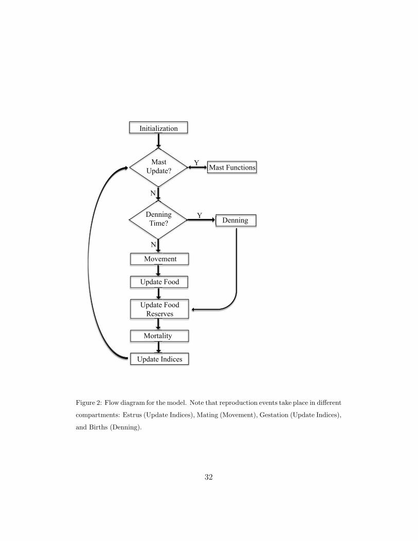
We analyzed data from live trapped black bears in Great Smoky Moun-

tains National Park using an open population estimator (Schwartz and Ar-

nason, 1996) in Program MARK (White and Burnham, 1999) to estimate

time-specific estimates of abundance. Figure 3 compares the 95% confidence

intervals for the IBM (solid) and mark-recapture estimates for males and

females in a sampling region in the NW quadrant of GSMNP. For males (A),

both sets of data show large fluctuations in the population and an overall

stable population. For females (B), both suggest smaller fluctuations and an

overall increase in the population.

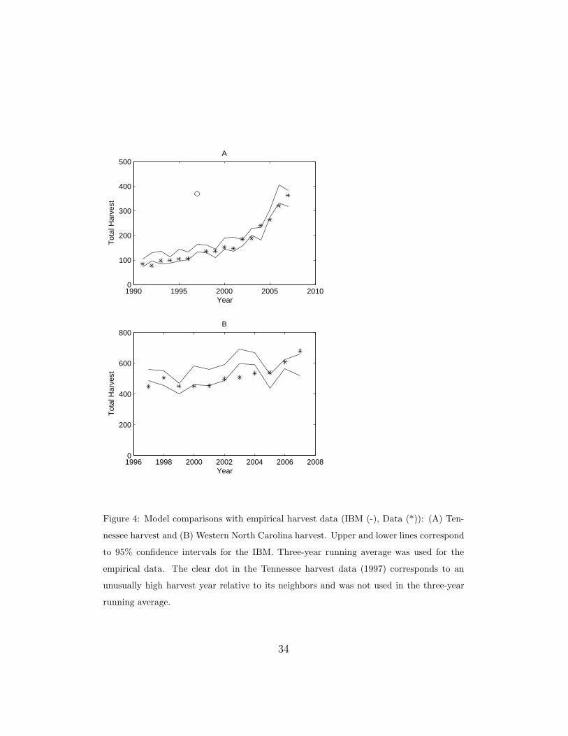
Figure 4 shows comparisons between empirical harvest data and model

output. Because the model assumes a constant harvest rate and cannot cap-

ture the annual variation in hunting effort associated with hunter behavior,

we took the three-year running average of the empirical data and compared

it to the 95% confidence intervals for the model. Graph (A) shows the Ten-

nessee harvest comparisons. The 1997 harvest data was a significant outlier

relative to the rest of the harvest data. Because the model cannot capture

that type of variation, we did not include it in the running average calcula-

tions. Although we did include it in the graph. The rapid increase in the

number of bears harvested after 2005 in Tennessee is due to the addition of

17

an archery season and an extended dog-hunting season. The model incor-

porated these changes by adding the new time periods for harvesting and

adjusting the harvest rate to account for the increased effort. Graph (B)

compares North Carolina harvest data with the model. The results indicate

that the model is capturing the magnitude of the harvest in both states.

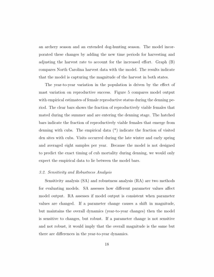
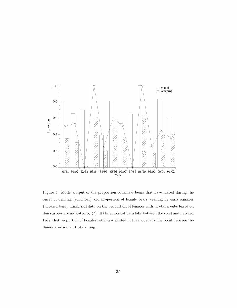
The year-to-year variation in the population is driven by the effect of

mast variation on reproductive success. Figure 5 compares model output

with empirical estimates of female reproductive status during the denning pe-

riod. The clear bars shows the fraction of reproductively viable females that

mated during the summer and are entering the denning stage. The hatched

bars indicate the fraction of reproductively viable females that emerge from

denning with cubs. The empirical data (*) indicate the fraction of visited

den sites with cubs. Visits occurred during the late winter and early spring

and averaged eight samples per year. Because the model is not designed

to predict the exact timing of cub mortality during denning, we would only

expect the empirical data to lie between the model bars.

3.2. Sensitivity and Robustness Analysis

Sensitivity analysis (SA) and robustness analysis (RA) are two methods

for evaluating models. SA assesses how different parameter values affect

model output. RA assesses if model output is consistent when parameter

values are changed. If a parameter change causes a shift in magnitude,

but maintains the overall dynamics (year-to-year changes) then the model

is sensitive to changes, but robust. If a parameter change is not sensitive

and not robust, it would imply that the overall magnitude is the same but

there are differences in the year-to-year dynamics.

18

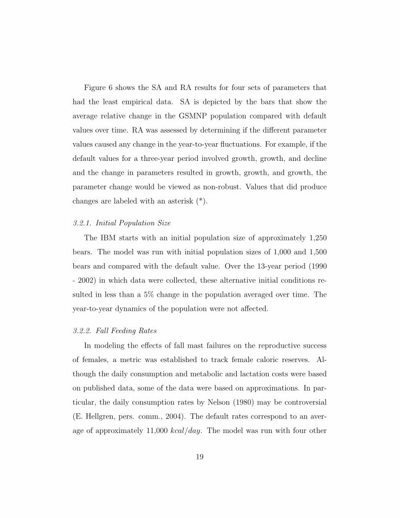
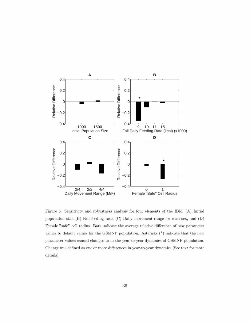
Figure 6 shows the SA and RA results for four sets of parameters that

had the least empirical data. SA is depicted by the bars that show the

average relative change in the GSMNP population compared with default

values over time. RA was assessed by determining if the different parameter

values caused any change in the year-to-year fluctuations. For example, if the

default values for a three-year period involved growth, growth, and decline

and the change in parameters resulted in growth, growth, and growth, the

parameter change would be viewed as non-robust. Values that did produce

changes are labeled with an asterisk (*).

3.2.1. Initial Population Size

The IBM starts with an initial population size of approximately 1,250

bears. The model was run with initial population sizes of 1,000 and 1,500

bears and compared with the default value. Over the 13-year period (1990

- 2002) in which data were collected, these alternative initial conditions re-

sulted in less than a 5% change in the population averaged over time. The

year-to-year dynamics of the population were not affected.

3.2.2. Fall Feeding Rates

In modeling the effects of fall mast failures on the reproductive success

of females, a metric was established to track female caloric reserves. Al-

though the daily consumption and metabolic and lactation costs were based

on published data, some of the data were based on approximations. In par-

ticular, the daily consumption rates by Nelson (1980) may be controversial

(E. Hellgren, pers. comm., 2004). The default rates correspond to an aver-

age of approximately 11,000 kcal/day. The model was run with four other

19

rates: 9,000, 10,000, 11,000, and 15,000. It was assumed that the rates were

constant throughout the fall. The results show that 9,000 kcal/day leads to

an essentially constant but low population size in which fall mast does not

determine the population size (i.e., not robust). A constant consumption

rate of 11,000 kcal/day was indistinguishable from the default rates. With a

consumption rate of 15,000 kcal/day, the population decreased, on average,

by 2% over the 13-year period. This was a result of bears needing more food

than is available which effectively decreased the carrying capacity.

3.2.3. Movement and Interaction Tolerance

Movement in the IBM were based on food availability. Bears moved to

the nearest cell with the most food. There were two components to this

movement: daily movement range and interaction tolerance.

The default values for daily movement range were a 4-cell radius for males

and a 2-cell radius for females (4/2). We compared the default values to 3

other sets of ranges: 2/4, 2/2, and 4/4. Female movement range was the

most sensitive parameter, but the model was robust to those changes.

In modeling interaction tolerance, the model assumed a “safe” cell radius

in which a bear can move into a cell. Results suggest that the model is

highly sensitive to the female interaction value. There was a 25% drop in the

population when the female interaction value was equal to 1 (default = 0).

This increased spacing forced more females to emigrate from the park. This

reduction in female bears resulted in a decreased effect of mast variation on

the population (smaller density). Because data supports the smaller terri-

torial association of female bears, the default assumptions provide a good

representation of the system.

20

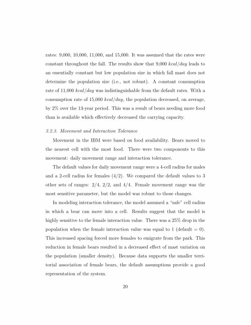
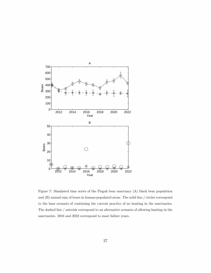
3.3. Example of Spatial Control

To look at the effects of alternative harvesting strategies on potential

bear-human encounters, we projected a mast time series through 2022. In

Figure 7, plot (A) shows the black bear population time series for the Pisgah

bear sanctuary. The solid line corresponds to the base scenario in which we

maintain the current harvesting regulations (no hunting in the sanctuaries)

while the dashed line shows a scenario that allows hunting. Plot (B) shows

the number of bears (summed over the year) in human-populated areas for

the no hunting (circle) and hunting (asterisk) strategies. The high circle val-

ues correspond to fall mast failure years. Note that opening the sanctuary to

hunting eliminated the bear-human encounters by decreasing the population

to a sustainable level.

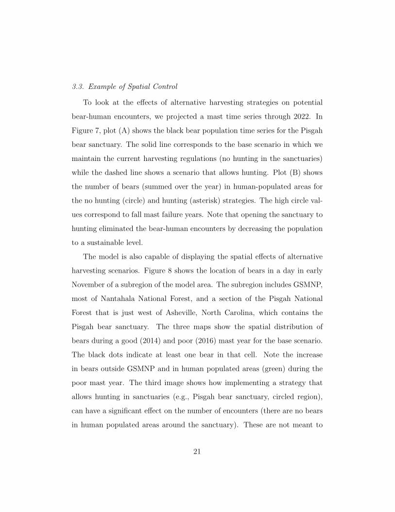
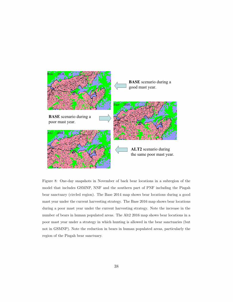
The model is also capable of displaying the spatial effects of alternative

harvesting scenarios. Figure 8 shows the location of bears in a day in early

November of a subregion of the model area. The subregion includes GSMNP,

most of Nantahala National Forest, and a section of the Pisgah National

Forest that is just west of Asheville, North Carolina, which contains the

Pisgah bear sanctuary. The three maps show the spatial distribution of

bears during a good (2014) and poor (2016) mast year for the base scenario.

The black dots indicate at least one bear in that cell. Note the increase

in bears outside GSMNP and in human populated areas (green) during the

poor mast year. The third image shows how implementing a strategy that

allows hunting in sanctuaries (e.g., Pisgah bear sanctuary, circled region),

can have a significant effect on the number of encounters (there are no bears

in human populated areas around the sanctuary). These are not meant to

21

suggest exact numbers or locations of bears during mast failure years, only

to represent a difference between abundant mast and mast failure years.

4. Discussion

4.1. Model Accuracy

We created an IBM of the black bear population of the southern Ap-

palachians to assist in the analysis of some of the growing concerns for this

population, particularly bear-human interactions. The flexibility of the IBM

allowed us to evaluate the model with the available empirical data sets. Based

on these evaluations, we conclude that the size, growth, and dynamics of the

model are realistic representations of population dynamics.

Despite the very encouraging evaluation results, the model has many

limitations. Two elements in the model with little empirical backing were

movement and caloric dynamics. We did not attempt to model all aspects

of bear movements explicitly. The movement rules in the model focus on

the effective movement dynamics for food consumption. Because there is

substantial home-range overlap among black bears (van Manen, 1994), the

spacing assumptions in the model seem to capture the general dynamics of

movement. The metabolic dynamics of reproductive females during fall are

a generalization of the actual dynamics. The lack of data for black bears

with similar diets and limitations in estimating mast availability led to these

simplifying assumptions. At some point between the onset of denning and

early summer movements, substantial cub mortality can occur, especially

after fall mast failures. Given the comparisons with empirical data not used

in developing the model or its parameters, we argue that our assumptions

22

are acceptable for applications of the model similar to the situations we

investigate.

4.2. Model Output

Models are often used for prediction. IBMs have the additional capabil-

ity of filling gaps in data to elucidate mechanisms for population dynamics.

Managers know that Fall hard mast variation is the main driver of black bear

population dynamics in the southern Appalachians, and limited data sug-

gests that fall mast affects movement and reproductive success. Our model

was able to provide further insight into how fall mast affects the black bear

population.

Figure 3 suggests a two-year decline in the population after a fall mast fail-

ure. The initial decline is caused by the movement of bears outside GSMNP

to search for food. The fraction of these bears that return to GSMNP is

unknown. The IBM can be used to extract life history data, like demograph-

ics, from these migrating bears and provide insight into how many of them

return. The second decline is associated with the loss of cubs during the

denning period following the mast failure. Because there is no new cohort,

the population declines, which becomes evident the second year. Because

most females will lose their cubs in years of severe mast failures, females are

able to reproduce again in the following summer. These females, coupled

with the females who just let their yearlings go, will all go into estrus that

summer resulting in reproductive synchrony. This has been seen empirically

(Figure 5). The effect is to produce a new large cohort three years after a

mast failure. Because of mortality, this synchrony is dampened over time

until the next hard mast failure. The IBM can be used to explore the long

23

term effects of these chort shifts on the population dynamics.

4.3. Model Applications

We demonstrated how the model can be used to look at the effects of

harvesting strategies on potential bear-human interactions. We focused on

how opening a bear sanctuary (Pisgah) to hunting would not eradicate the

population, but would maintain it at a level that would reduce potential

bear-human encounters. The IBM can be used to address the effectiveness

of individual sanctuaries with respect to size and location. For example,

what is the minimum size for a sanctuary so that it can maintain a source

population, or is an effective sanctuary size a function of its proximity to

another sanctuary? More specifically, spatial control problems related to the

location, magnitude, and timing of harvesting can be tested using the IBM.

Because of the versatility associated with IBMs, many other issues can

be addressed with this model. For a long-term perspective, the model can be

used to investigate how global warming might effect the black bear population

via changes in mast production. The model can also give managers better

insights into the population dynamics of the black bear population with

emphasis on demographics and movement among regions.

5. Acknowledgements

We thank NSF Award DMS - 0110920 to the University of Tennessee at

Knoxville for supporting this work. This work was assisted by attendance as

a Short-term Visitor at the National Institute for Mathematical and Biolog-

ical Synthesis, an Institute sponsored by the National Science Foundation,

the U.S. Department of Homeland Security, and the U.S. Department of

24

Agriculture through NSF Award EF-0832858, with additional support from

The University of Tennessee, Knoxville. Also, special thanks to Dr. Scott

Duke-Sylvester for help in the early process of developing the code and Bill

Stiver with the National Park Service at Great Smoky Mountains National

Park.

References

Beeman, L., Pelton, M., 1970. Seasonal foods and feeding ecology of the black

bear in the Smoky Mountains. Int. C. Bear 2, 75–107.

Brody, A., Pelton, M., 1988. Seasonal changes in digestion in black bears.

Can. J. Zoolog. 66, 1482–1484.

Burton, T., Koch, D., Updike, D., Brody, A., 1994. Evaluation of the poten-

tial effects of sport hunting on California black bears. Int. C. Bear 9 (1),

231–235.

Carr, P., 1983. Habitat utilization and seasonal movement of black bears in

the Great Smoky Mountains National Park. Master’s thesis, University of

Tennessee, Knoxville.

Clark, J., van Manen, F. T., Pelton, M. R., 2005. Bait stations, hard mast,

and black bear population growth in Great Smoky Mountains National

Park. J. Wildlife Manage. 69 (4), 1633–1640.

Costello, C., 2010. Estimates of dispersal and home-range fidelity in Ameri-

can black bears. J. Mammal. 91 (1), 116–121.

25

Darley-Hill, S., Johnson, W., 1981. Acorn dispersal by the blue jay

(cyanocitta cristata). Oecologia 50, 231–232.

DeAngelis, D., Gross, L., 1992. Individual-based Models and Approaches in

Ecology: Populations, Communities, and Ecosystems. Chapman and Hall.

Decker, D., Chase, L., 1997. Human dimensions of living with wildlife-

management challenge for the 21st century. Wildlife Soc. B. 25 (4), 788–

795.

Delozier, E. K., Stiver, W. H., 2005. Great Smoky Mountains National Park

black bear status report. In: 18th Black Bear Workshop. pp. 114–117.

Dente, C. R., Renar, E. A., 2005. New York black bear status report. In:

18th Black Bear Workshop. pp. 75–81.

Eagle, T., Pelton, M., 1981. Seasonal nutrition of black bears in the Great

Smoky Mountains National Park. Int. C. Bear 5, 94–101.

Eiler, J., Wathen, W. G., Pelton, M., 1989. Reproduction in black bears in

the southern Appalachian Mountains. J. Wildlife Manage. 53, 353–360.

Farley, S., Robbins, C., 1995. Lactation, hibernation and mass dynamics of

american black bears and grizzly bears. Can. J. Zoolog. 73, 2216–2222.

Greenberg, C., 2000. Individual variation in acorn production by five species

of southern Appalachian oaks. Forest Ecol. Manage. 132, 199–210.

Grimm, V., Berger, U., Bastiansen, F., Eliassen, S., Ginot, V., Giske, J.,

Goss-Custard, J., Grand, T., Heinz, S., Huse, G., Huth, A., Jepsen, J.,

26

Jørgensen, C., Mooij, W., Mller, B., Pe’er, G., Piou, C., Railsback, S.,

Robbins, A., Robbins, M., Rossmanith, E., Rger, N., Strand, E., Souissi,

S., Stillman, R., Vab, R., Visser, U., DeAngelis, D., 2006. A standard

protocol for describing individual-based and agent based models. Ecol.

Model. 198, 115–126.

Grimm, V., Railsback, S., 2005. Individual-based Modeling and Ecology.

Princeton University Press.

Hilderbrand, G., Jenkins, S., Schwartz, C., Hanley, T., Robbins, C., 1999.

Effects of seasonal differences in dietary meat intake on changes in body

mass and composition in wild and captive brown bears. Can. J. Zoolog.

77, 1623–1630.

Inman, R. M., Pelton, M. R., 2002. Energetic production by soft and hard

mast foods of American black bears in the Smoky Mountains. Ursus 13,

111–126.

Koenig, W., Knops, J., 2000. The behavioral ecology of masting in oaks. In:

McShea, W., Healy, W. (Eds.), Oak Forest Ecosystems. Johns Hopkins

University, pp. 129 – 148.

Martin, D., Steffen, D., 2005. Virginia black bear status report. In: 18th

Black Bear Workshop. pp. 136–150.

Maxwell, R., Thornkelson, J., Rogers, L., Brander, R., 1988. The field en-

ergetics of winter-dormant black bear in northeastern Minnesota. Can. J.

Zoolog. 66, 2095–2103.

27

McCullough, D., 1996. Spatially structured populations and harvest theory.

J. Wildlife Manage. 60 (1), 1–9.

McLean, P., 1991. The demographic and morphological characteristics of

black bears in the Smoky Mountains. Ph.D. thesis, University of Tennessee,

Knoxville.

Mclean, P., Pelton, M., 1994. Estimates of population density and growth of

black bears in the Smoky Mountains. Int. C. Bear 9, 253–261.

Miller, S., 1992. Population management of bears in North America. Int. C.

Bear 8, 357–373.

Nelson, R., Jr., G. F., Pfeiffer, E., Craighead, J., Jonkel, C., Steiger, D.,

1980. Behavior, biochemistry, and hibernation in black, grizzly, and polar

bears. Int. C. Bear 5, 284–290.

Powell, R., 1987. Black bear home range overlap in North Carolina and the

concept of home range applied to black bears. Int. C. Bear 7, 235–242.

Powell, R., Zimmerman, J., Seaman, D., 1997. Ecology and behavior of

North American black bears: home ranges, habitat, and social organi-

zation. Chapman & Hall.

Pritchard, G., Robbins, C., 1990. Digestive and metabolic efficiencies of griz-

zly and black bears. Can. J. Zoolog. 68, 1645–1651.

Quigley, H., 1982. Activity patterns, movement ecology, and habitat utiliza-

tion of black bears in the Great Smoky Mountains National Park, Ten-

nessee. Master’s thesis, University of Tennessee, Knoxville.

28

Rogers, L., 1987. Effects of food supply and kinship on social behavior, move-

ments, and population growth of black bears in northeastern Minnesota.

Wildlife Monogr. 97.

Ryan, C. W., 2005. West Virginia black bear status report. In: 18th Black

Bear Workshop. pp. 151–158.

Schoen, J., 1992. Bear habitat management: A review and future perspective.

Int. C. Bear 8, 143–154.

Schwartz, C. J., Arnason, A. N., 1996. A general methodology for the analysis

of capture-recapture experiments in open populations. Biometrics 52, 860–

873.

Steiner, K., 1996. Autumn predation of northern red oak seed crops. In:

Gottschalk, K., Fosbroke, S. (Eds.), 10th Central hardwood forest confer-

ence. U.S. Forest Service General Technical Report NE-197, pp. 489–494.

Timmins, A. A., 2005. New Hampshire black bear status report. In: 18th

Black Bear Workshop. pp. 63–74.

van Manen, F., 1994. Black bear habitat use in the Great Smoky Mountains

National Park. Ph.D. thesis, University of Tennessee, Knoxville.

Watts, P., Oritsland, N., Jonkel, C., Ronald, K., 1981. Mammalian hiberna-

tion and the oxygen consumption of a denning black bear. Comp. Biochem.

Physiol. 69a, 121.

Weigand, T., Naves, J., Stephan, T., Fernandez, A., 1998. Assessing the risk

29

of extinction for the brown bear in the Cordillera Cantabrica, Spain. Ecol.

Monogr. 68 (4), 539–570.

White, G. C., Burnham, K. P., 1999. Program mark: survival estimation

from populations of marked animals. Bird Study 46 Supplement, 120–138.

Yodzis, P., Kolenosky, G., 1986. A population dynamics model for black bear

in eastcentral Ontario. J. Wildlife Manage. 50 (4), 602–612.

30

GSMNP

CNF

PNF

NNF

Bear Sanctuaries

Human Population

Figure 1: The eastern Tennessee and western North Carolina region used in the model.

31

Initialization

Denning

Mast

Update?

Denning

Time?

Update Food

Reserves

Update Food

Movement

Mortality

Update Indices

Mast Functions

Y

Y

N

N

Figure 2: Flow diagram for the model. Note that reproduction events take place in different

compartments: Estrus (Update Indices), Mating (Movement), Gestation (Update Indices),

and Births (Denning).

32

1988 1990 1992 1994 1996 1998 2000 20020

100

200

300

400

Year

Pop

ulat

ion

Siz

e

A

1988 1990 1992 1994 1996 1998 2000 20020

50

100

150

200

Year

Pop

ulat

ion

Siz

e

B

Figure 3: (A) 95% CIs for POPAN population estimate for males in the NW sampling

region of GSMNP(Dash-dotted) and IBM output (solid line) and (B) corresponding female

data.

33

1990 1995 2000 2005 20100

100

200

300

400

500A

Year

Tot

al H

arve

st

1996 1998 2000 2002 2004 2006 20080

200

400

600

800B

Year

Tot

al H

arve

st

Figure 4: Model comparisons with empirical harvest data (IBM (-), Data (*)): (A) Ten-

nessee harvest and (B) Western North Carolina harvest. Upper and lower lines correspond

to 95% confidence intervals for the IBM. Three-year running average was used for the

empirical data. The clear dot in the Tennessee harvest data (1997) corresponds to an

unusually high harvest year relative to its neighbors and was not used in the three-year

running average.

34

90/91 91/92 92/93 93/94 94/95 95/96 96/97 97/98 98/99 99/00 00/01 01/02 Year

0.0

0.2

0.4

0.6

0.8

1.0

Prop

ortio

n

MatedWeaning

Figure 5: Model output of the proportion of female bears that have mated during the

onset of denning (solid bar) and proportion of female bears weaning by early summer

(hatched bars). Empirical data on the proportion of females with newborn cubs based on

den surveys are indicated by (*). If the empirical data falls between the solid and hatched

bars, that proportion of females with cubs existed in the model at some point between the

denning season and late spring.

35

1000 1500−0.4

−0.2

0

0.2

0.4A

Initial Population Size

Rel

ativ

e D

iffer

ence

9 10 11 15−0.4

−0.2

0

0.2

0.4

*

B

Fall Daily Feeding Rate (kcal) (x1000)

Rel

ativ

e D

iffer

ence

2/4 2/2 4/4−0.4

−0.2

0

0.2

0.4C

Daily Movement Range (M/F)

Rel

ativ

e D

iffer

ence

0 1−0.4

−0.2

0

0.2

0.4

*

D

Female "Safe" Cell Radius

Rel

ativ

e D

iffer

ence

Figure 6: Sensitivity and robustness analysis for four elements of the IBM. (A) Initial

population size, (B) Fall feeding rate, (C) Daily movement range for each sex, and (D)

Female ”safe” cell radius. Bars indicate the average relative difference of new parameter

values to default values for the GSMNP population. Asterisks (*) indicate that the new

parameter values caused changes to in the year-to-year dynamics of GSMNP population.

Change was defined as one or more differences in year-to-year dynamics (See text for more

details).

36

2012 2014 2016 2018 2020 20220

100

200

300

400

500

600

700

Bea

rs

Year

A

2012 2014 2016 2018 2020 20220

10

20

30

40

50

Bea

rs

Year

B

Figure 7: Simulated time series of the Pisgah bear sanctuary (A) black bear population

and (B) annual sum of bears in human-populated areas. The solid line / circles correspond

to the base scenario of continuing the current practice of no hunting in the sanctuaries.

The dashed line / asterisk correspond to an alternative scenario of allowing hunting in the

sanctuaries. 2016 and 2022 correspond to mast failure years.

37

BASE scenario during a

good mast year.

BASE scenario during a

poor mast year.

ALT2 scenario during

the same poor mast year.

Figure 8: One-day snapshots in November of back bear locations in a subregion of the

model that includes GSMNP, NNF and the southern part of PNF including the Pisgah

bear sanctuary (circled region). The Base 2014 map shows bear locations during a good

mast year under the current harvesting strategy. The Base 2016 map shows bear locations

during a poor mast year under the current harvesting strategy. Note the increase in the

number of bears in human populated areas. The Alt2 2016 map shows bear locations in a

poor mast year under a strategy in which hunting is allowed in the bear sanctuaries (but

not in GSMNP). Note the reduction in bears in human populated areas, particularly the

region of the Pisgah bear sanctuary.

38

Table 1: State variables for the model divided into individual and landscape level designations.

State Variable Units Description

Individual Bears

Age Days Bear’s age in days

Sex M/F Determined at birth with 1:1 ratio

Location (x,y) Coordinates based on cell location

Denning flag 0/1 Flags a denning individual

Denning days Days Daily counter to determine den emergence (see text)

Estrus flag 0/1 Flags a female in estrus

Estrus days Days Daily counter to determine mating (see text)

Weaning flag 0/1 Flags a female weaning cubs

Fall caloric reserves kilocalories (kcal) Food intake minus kilocalories burned (see text)

ID number Integer Non-repeating integer values to ID individuals

Mother’s ID Integer ID of an individual’s mother

Lanscape cells

State Integer Tennessee or North Carolina

Region Integer GSMNP or one of the National Forests (see Figure 1)

Sanctuary Integer Identifies whether a cell can be hunted

Human population People

km2 Human population density

Vegetation class Integer Vegetation type for each cell (See Table 2)

Kilocalories kcal Kilocalories available minus amount consumed (see text)

Bear Population Integer The total number of bears in a cell

39

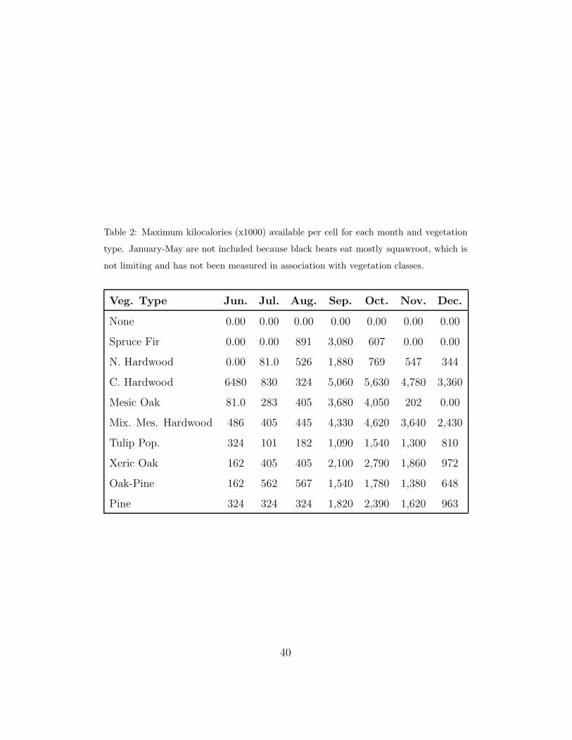
Table 2: Maximum kilocalories (x1000) available per cell for each month and vegetation

type. January-May are not included because black bears eat mostly squawroot, which is

not limiting and has not been measured in association with vegetation classes.

Veg. Type Jun. Jul. Aug. Sep. Oct. Nov. Dec.

None 0.00 0.00 0.00 0.00 0.00 0.00 0.00

Spruce Fir 0.00 0.00 891 3,080 607 0.00 0.00

N. Hardwood 0.00 81.0 526 1,880 769 547 344

C. Hardwood 6480 830 324 5,060 5,630 4,780 3,360

Mesic Oak 81.0 283 405 3,680 4,050 202 0.00

Mix. Mes. Hardwood 486 405 445 4,330 4,620 3,640 2,430

Tulip Pop. 324 101 182 1,090 1,540 1,300 810

Xeric Oak 162 405 405 2,100 2,790 1,860 972

Oak-Pine 162 562 567 1,540 1,780 1,380 648

Pine 324 324 324 1,820 2,390 1,620 963

40