Current and Future Challenges in Mathematical and Computational Biology

Louis J. GrossThe Institute for Environmental ModelingDepartments of Ecology and Evolutionary

Biology and MathematicsUniversity of Tennessee

ATLSS.orgwww.nih.gov

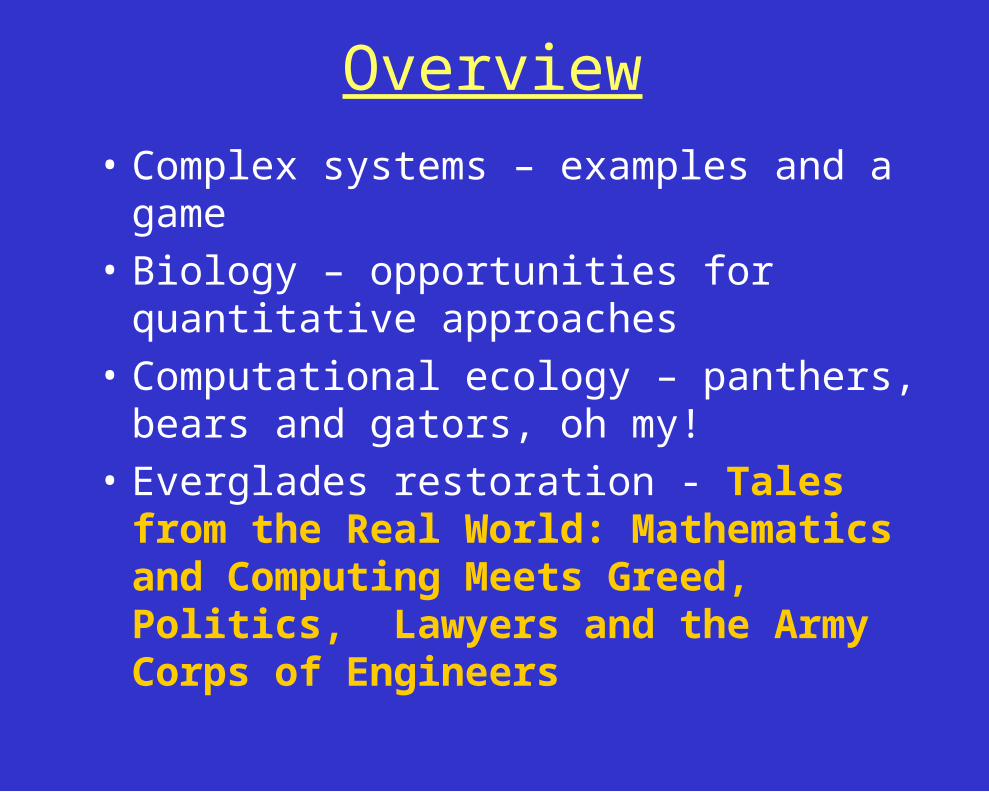
Overview• Complex systems – examples and a game• Biology – opportunities for quantitative

approaches• Computational ecology – panthers, bears

and gators, oh my! • Everglades restoration - Tales from

the Real World: Mathematics and Computing Meets Greed, Politics, Lawyers and the Army Corps of Engineers

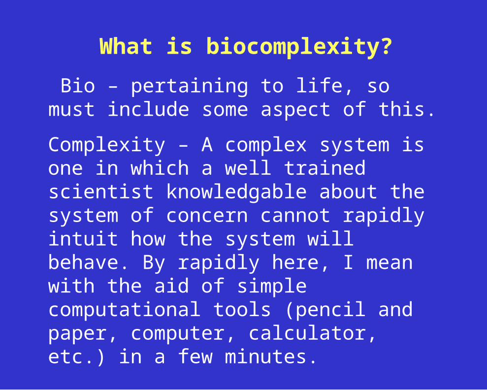
What is biocomplexity?

Bio – pertaining to life, so must include some aspect of this.

Complexity – A complex system is one in which a well trained scientist knowledgable about the system of concern cannot rapidly intuit how the system will behave. By rapidly here, I mean with the aid of simple computational tools (pencil and paper, computer, calculator, etc.) in a few minutes.

Routes to complexity

Complexity should include systems that may be quite easily described, but have underlying complicated responses (e.g. the chaotic dynamics models of single or multiple populations) that one cannot intuit easily, as well as systems that most of us would agree are complicated due to multiple interacting factors (food webs with many components, ecosystems with dynamic and spatial responses on multiple scales).

Music courtesy of Steve Kaufman, 3-time National Flatpicking champion

What is going on here?• This is an example of a Polya Urn scheme• If you think of what is happening in one particular cup,

this corresponds to the sample path or trajectory for a Stochastic Process (a collection of random variables, Xn which give the number of blue beads in the cup at time n)

• Each cup (or sample path) is independent of the others, and we describe the whole process by looking at the collection of sample paths at each time, and calculate the fraction of these having a particular value – this gives a histogram that describes the probability distribution at each time.

• We can simulate this and we see that each sample path approaches a particular fraction of beans in the cup of a particular color.

• When we look across all cups after a long period of time we see that the histogram approaches a particular distribution – in the case we did it is the Uniform distribution – each possible fraction between 0 and 1 is equally likely.

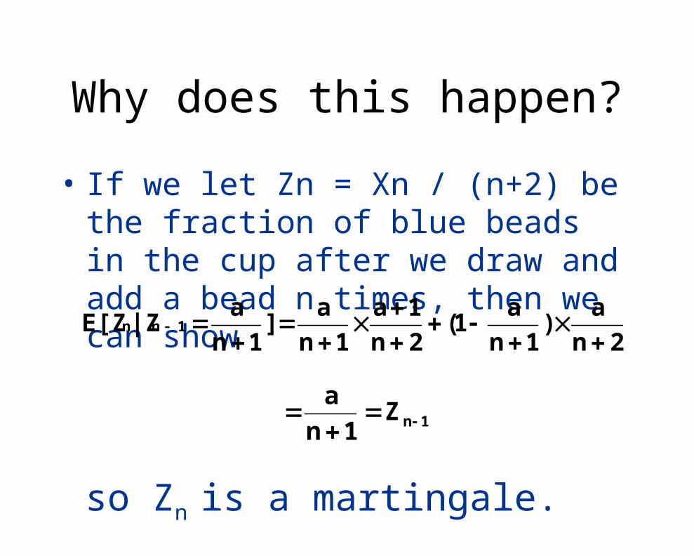
Why does this happen?

• If we let Zn = Xn / (n+2) be the fraction of blue beads in the cup after we draw and add a bead n times, then we can show

2na)

1na1(

2n1a

1na]

1na|ZE[Z 1nn

1nZ1n

a

so Zn is a martingale.

A martingale can be proved to have a limiting distribution so that

ZZlim nn

Where Z is the limiting random variable and it’s distribution is called the limiting distribution – this is the Uniform distribution in our cup experiment.

1

4

7

10S1

S4S7

S10

0

0.1

0.2

0.3

Urn Schemes and Null Models:

Cohen, Joel E. 1976. Irreproducible Results and the Breeding of Pigs (or Nondegenerate Limit Random Variables in Biology). BioScience 26:391-394.

For an ecological example of extensions of these ideas see The Unified Neutral Theory of Biodiversity and Biogeography. Stephen P. Hubbell. Princeton University Press. 2001.

For an evolutionary theory example of extensions see Gavrilets, S, R. Acton and J. Gravner. 2000. Dynamics of speciation and diversification in a metapopulation. Evolution 54:1493-1501

What is computational ecology?

An interdisciplinary field devoted to the quantitative description and analysis of ecological systems using empirical data, mathematical models (including statistical models), and computational technology. Focus includes: Data Management, Modeling, and Visualization (Helly et al., 1995)

Computational Ecology

• How do population and community properties arise from individual behaviors?

• How does spatial and temporal heterogeneity affect population and communities?

• How are distribution and abundance of species linked to spatio-temporal patterns of evolution?

• How do we link dynamic models with spatial data to aid natural system monitoring and management, including reserve design, water flow control, and harvesting schedules?

• How do we include socio-economic analysis with ecological models?

Theory development Applications

Environmental Modeling

Data sources

Models

Management input

Monitoring

Simulation Analysis

GIS map layers (Vegetation, hydrology, elevation),Weather, Roads, Species densities

Statistical

Differential equations

Matrix

Agent-based

Matlab, C++, Distributed, ParallelVisualization, corroboration, sensitivity, uncertainty

Harvest regulation

Water control

Reserve design

Species densities

Animal telemetry

Physical conditions

Overview• Everglades natural history• History of hydrology in South Florida• Restoration planning• Computational ecology

– Multimodeling– The ATLSS project and Everglades restoration

• Problems in spatial control– Reserves and individual-based models– Managing antibiotic resistance– Theory and intercropping

• What are some future challenges?

Key Points• Realistic modeling of natural systems requires

multiple linked approaches – multimodeling - and new methods are needed to develop and analyze these.

• Much of applied ecology deals with problems of spatial control – what to do, where to do it, when to do it, and how to monitor it – and these problems are not easily solved, opening up many new, fascinating problems in applied mathematics and computational science.

• It can be very rewarding for mathematicians to get involved in “big” multidisciplinary problems

Photos: South Florida Water Management District

Dry Season: November-April

Wet Season:May-October

Everglades Restoration

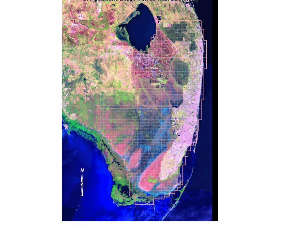
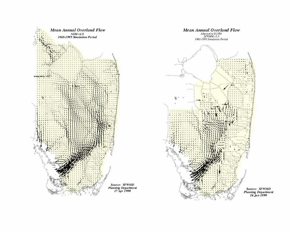
The Everglades and Big Cypress Swamp of South Florida are characterized by complex patterns of spatial heterogeneity and temporal variability, with water flow being the major factor controlling the trophic dynamics of the system. A key objective of modeling studies for these systems is to compare the future effects of alternative hydrologic scenarios on the biotic components of the systems.

Recent History of Everglades Restoration

C&SF Project facilities developed since 1940’s include 30 pumping stations, 212 control and diversion structures, 990 miles of levees, 978 miles of canals, 25 navigation locks, and 56 railroad bridges.

1992 - Congress authorizes Comprehensive Review Study (Restudy) of the C&SF Project to develop modifications to restore the Everglades and Florida Bay ecosystems while providing for the other water-related needs of the region.

1999 - Restudy Plan submitted to Congress on July 1. Restudy Objective: Develop a comprehensive plan for implementing changes needed to meet water supply needs through 2050 and restore over 2.4 million acres of the greater Everglades ecosystem

Agencies involved in Restudy: U.S. Army Corps of Engineers Environmental Protection Agency National Park Service National Marine Fisheries Service Natural Resources Conservation Service U.S. Fish and Wildlife Service Florida Department of Agriculture and Consumer Services Florida Department of Environmental Protection Florida Game and Fresh Water Fish Commission South Florida Water Management District Miccosukee Tribe Seminole Tribe plus input from numerous NGO's and individuals.

Plan includes:Reconnecting over 80 percent of the remaining Everglades by removing over 240 miles of internal levees and canals.

Reduce the average of 1.7 billion gallons of water wasted every day from discharges to the ocean

Additional land purchases of 47,000 acres as an addition to ENP

Approximate cost: $7.8 Billion over 20 years

What is computationally challenging in this?

• Space-time linkages• GIS very limited at dynamic modeling• Different components operate on different scales

(resolution required differs between components)• Model data can be huge

• Models are complex• Large state variable dynamical systems• Large numbers of interconnected agents• Models are not independent - multimodeling

Everglades natural system management requires decisions on short time periods about what water flows to allow where and over longer planning horizons how to modify the control structures to allow for appropriate controls to be applied.

•The control objectives are unclear and differ with different stakeholders.•Natural system components are poorly understood.•The scales of operation of the physical system models are coarse.

This is very difficult!

So what have we done?

Developed a multimodel (ATLSS - Across Trophic Level System Simulation) to link the physical and biotic components.Compare the dynamic impacts of alternative hydrologic plans on various biotic components spatially.Let different stakeholders make their own assessments of the appropriate ranking of alternatives.

http://atlss.org

What ATLSS attempts to do

• Provide a general methodology for regional assessment of natural systems by coupling physical and biotic processes in space and time using a mixture of modeling approaches.

• Utilize the best available science and intuition of many biologists with extensive field experience to construct models for particular system components and link these at appropriate spatial and temporal resolutions

What ATLSS attempts to do (con’d)

• Provide a method to compare the relative impacts of alternative management of the region on the natural systems, so different stakeholders can focus on sub-regions, species, or conditions of particular interest to them.

• Ensure that the structure of the multimodel is extensible so that as new models, data and monitoring information becomes available, it may be efficiently utilized.

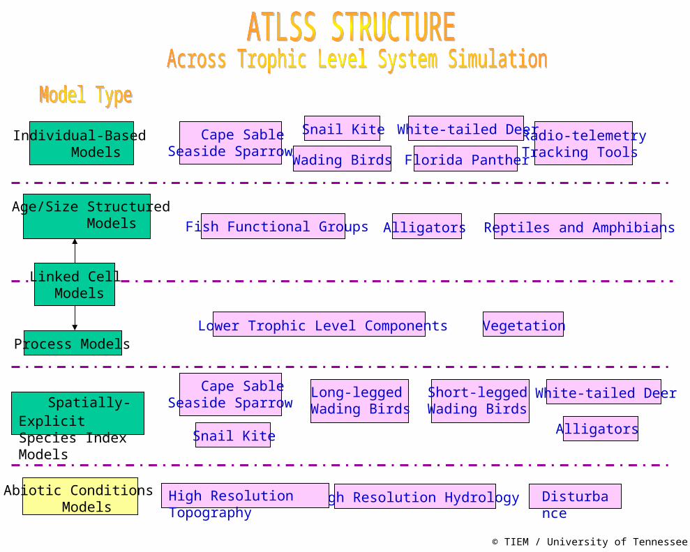
Radio-telemetryTracking Tools

Abiotic Conditions Models

Spatially-Explicit Species Index Models

Linked Cell Models

Process Models

Age/Size Structured Models

Individual-Based Models

High Resolution HydrologyHigh Resolution Topography Disturbance

Cape Sable Seaside Sparrow

Snail Kite

Long-legged Wading Birds

Short-legged Wading Birds

White-tailed Deer

Alligators

Lower Trophic Level Components Vegetation

Fish Functional Groups Alligators Reptiles and Amphibians

White-tailed Deer

Florida Panther

Snail Kite

Wading Birds

© TIEM / University of Tennessee 1999

Cape Sable Seaside Sparrow

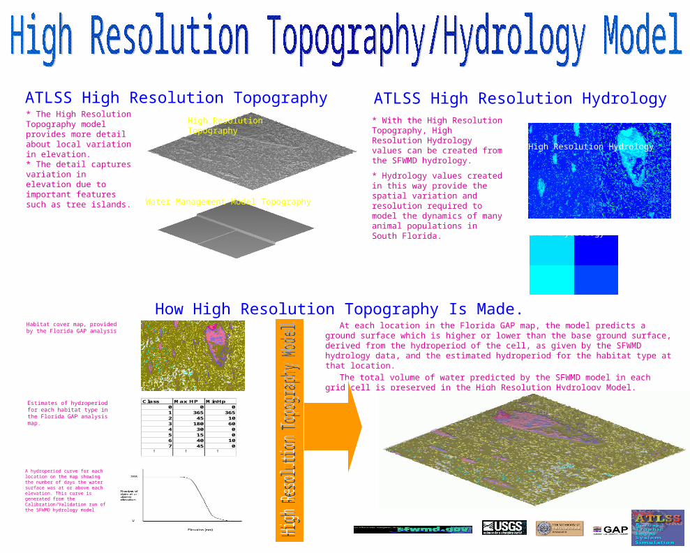
ATLSS High Resolution TopographyHigh Resolution Topography

* The High Resolution Topography model provides more detail about local variation in elevation.* The detail captures variation in elevation due to important features such as tree islands.

ATLSS High Resolution Hydrology* With the High Resolution Topography, High Resolution Hydrology values can be created from the SFWMD hydrology.

* Hydrology values created in this way provide the spatial variation and resolution required to model the dynamics of many animal populations in South Florida.

High Resolution Hydrology

SFWMD Hydrology

How High Resolution Topography Is Made.

Class Max HP MinHp0 0 01 365 3652 45 103 180 604 30 05 15 06 40 107 45 0…

.

….

….

Habitat cover map, provided by the Florida GAP analysis

Estimates of hydroperiod for each habitat type in the Florida GAP analysis map.

A hydroperiod curve for each location on the map showing the number of days the water surface was at or above each elevation. This curve is generated from the Calibration/Validation run of the SFWMD hydrology model.

At each location in the Florida GAP map, the model predicts a ground surface which is higher or lower than the base ground surface, derived from the hydroperiod of the cell, as given by the SFWMD hydrology data, and the estimated hydroperiod for the habitat type at that location.

The total volume of water predicted by the SFWMD model in each grid cell is preserved in the High Resolution Hydrology Model.

Water Management Model Topography

4 miles

4 m

iles

4 miles

4 m

iles

4 miles4 miles

4 miles4 miles

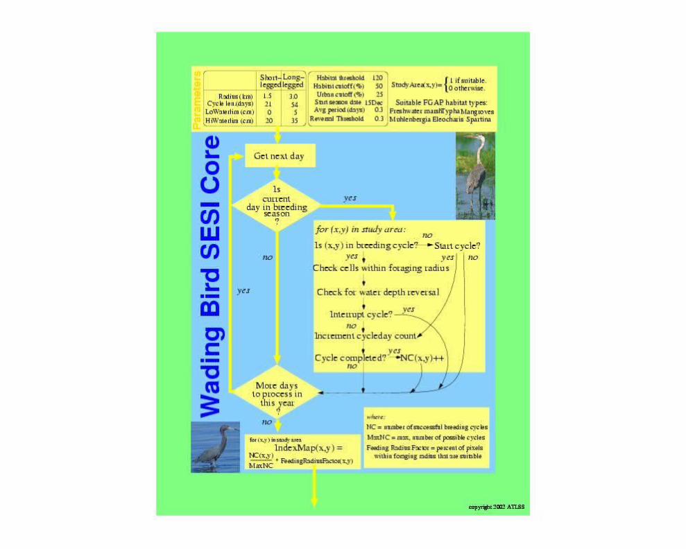
Spatially-Explicit Species Index (SESI) Models

The simplest of the ATLSS models, they are designed as extensions of habitat suitability index models, to provide yearly assessments of the effects of within and between year hydrology variation on basic requirements for foraging and breeding in a spatially-explicit manner. They allow comparisons of alternative scenarios, and allow different stakeholders to focus on their own criteria.

ATLSS SESI Models

Implement and Execute the Models for a Hydrology Scenario

Objectives: Integrate SESI components into a cohesive computational framework and apply the models to a hydrology scenario.

Hydrology Scenario

Distribute water over high resolutiontopography

Standard Output Generation/Visualization Tools

Daily Water Depth

Cape SableSeaside Sparrow

SnailKite

Wading Birds White-tailedDeer

AmericanAlligator

SESI ModelsHigh Resolution Hydrology

Are the nestsflooded duringegg incubation?

Is there high groundto build a nest on?

Is breeding disrupted byhigh waterlevels?

Are water depths inthe correct range forthe fish they eat?

Are conditionsfavorable for theapple snails theydepend on?

Fish biomass is one of the most important components of the Everglades system. To produce projections of fish biomass

ATLSS uses a... 

… spatially explicit size-structured dynamic simulation model, ALFISH.

 ALFISH simulates the number, size-structure and biomass

densities of “small fish” and “large fish” functional groups in the freshwater marsh on 5-day time steps.

 This represents the temporally and spatially varying food base

for wading birds. 

ALFISH has been evaluated through comparisons to some sites in Shark Slough and WCA3.

ATLSS Fish Functional Group Dynamics Model

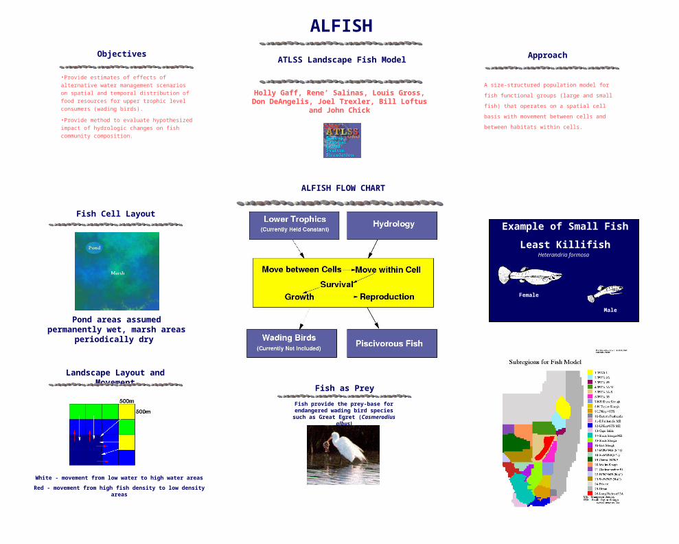
ATLSS Landscape Fish Model

ALFISH

Holly Gaff, Rene’ Salinas, Louis Gross, Don DeAngelis, Joel Trexler, Bill Loftus and John

Chick

Example of Small FishLeast Killifish

Heterandria formosa

Female

Male

ALFISH FLOW CHART

Objectives

•Provide estimates of effects of alternative water management scenarios on spatial and temporal distribution of food resources for upper trophic level consumers (wading birds).•Provide method to evaluate hypothesized impact of hydrologic changes on fish community composition.

A size-structured population model for fish functional groups (large and small fish) that operates on a spatial cell basis with movement between cells and between habitats within cells.

Approach

Fish provide the prey-base for endangered wading bird species

such as Great Egret (Casmerodius albus)

Fish as Prey

Fish Cell Layout

Pond areas assumed permanently wet, marsh areas

periodically dry

Landscape Layout and Movement

White - movement from low water to high water areasRed - movement from high fish density to low density

areas

Fish Available as Prey during a High Rainfall

Year

Fish Available as Prey during a Typical Rainfall

Year

Average Fish Available as Prey from 1965 - 1995

Distribution of Sizes for Fish in WCA 3A

Total Fish Densities through 31-year Model

Run

Total Fish Densities for Certain Years in Given

Areas

Average Fish Available as Prey during Breeding Season for Wading Birds

Fish Available as Prey during a Low Rainfall

Year

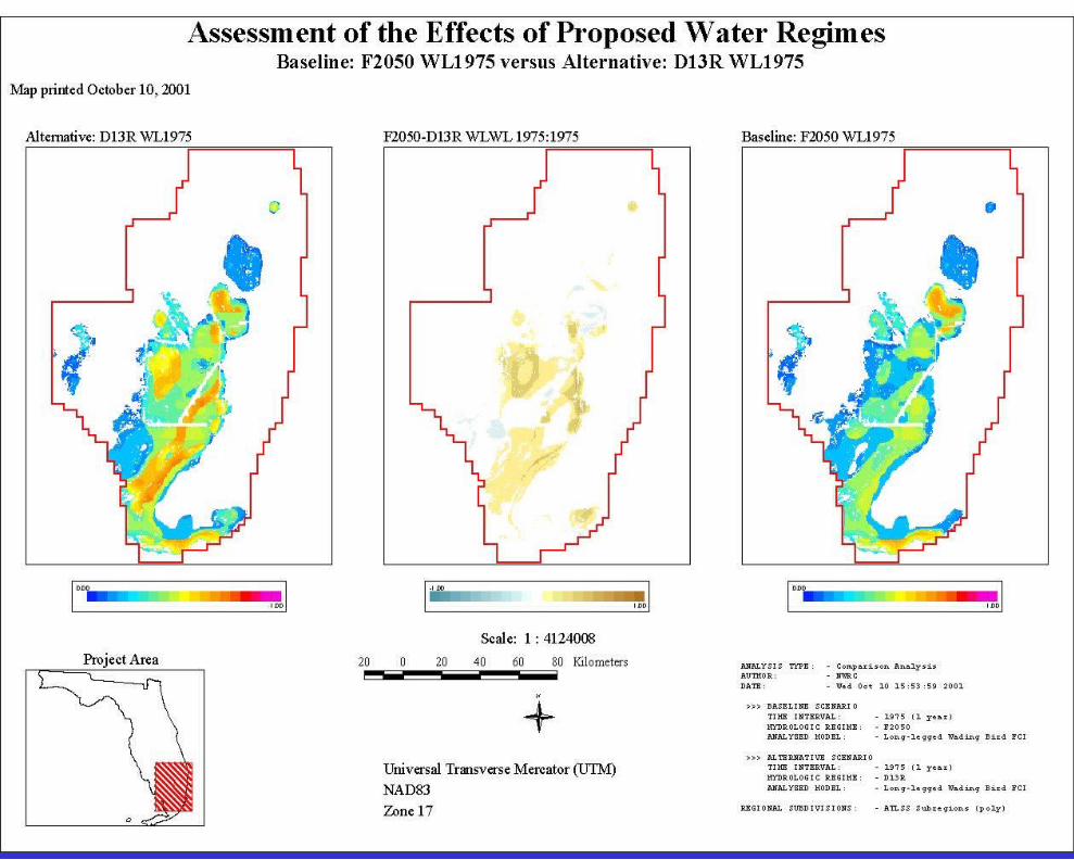
ALFISH MODEL EXAMPLE RESULTS - Alt D13r4 compared to F2050Base

 The ATLSS SESI models can provide considerable information

about spatial and temporal patterns of habitat conditions affecting breeding and foraging. They can indicate how one

scenario differs from another, but no demographics are included. To include demographics and thus project population-level

dynamics, ATLSS uses... 

… spatially explicit individual-based (SEIB) demographic models:

Snail kite, Cape Sable seaside sparrow, Florida panther/white-tailed deer

 These contain life cycle and behavioral information and they

allow the user to simulate population levels, structure and growth.

 

ATLSS Individual-Based Demographic Models

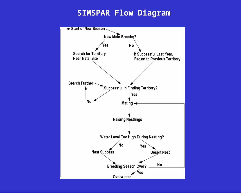
SIMSPAR Flow Diagram

Projected Population Size Fledgling Productivity

Maps

Take-Home Messages• Realistic modeling of natural systems requires multiple linked approaches –

multimodeling.• ATLSS has been successful in providing a flexible structure in which new

models can be included, and new data taken into account to modify existing models

• ATLSS has provided a rational approach, based upon the best available science, for providing multiple stakeholders with some of the tools they need to have input into regional planning

Collaborations in ATLSSIn addition to various Federal and State cooperators, ATLSShas involved researchers at

Florida International University   Southwestern Louisiana University   University of Florida University of Maryland   University of Miami University of Tennessee University of Washington National Wetland Research Center (USGS) The Institute for Bird Populations Everglades Research Group Netherlands Institute of Ecology

Some other spatial control problems•Bears and hunting preserves – an application of individual-based modeling (Rene’ Salinas)

•Controlling antibiotic resistance – numerically intensive spatial modeling (Scott Duke-Sylvester)

•Intercropping – a theoretical approach coupling reaction-diffusion and ODE models (Suzanne Lenhart)

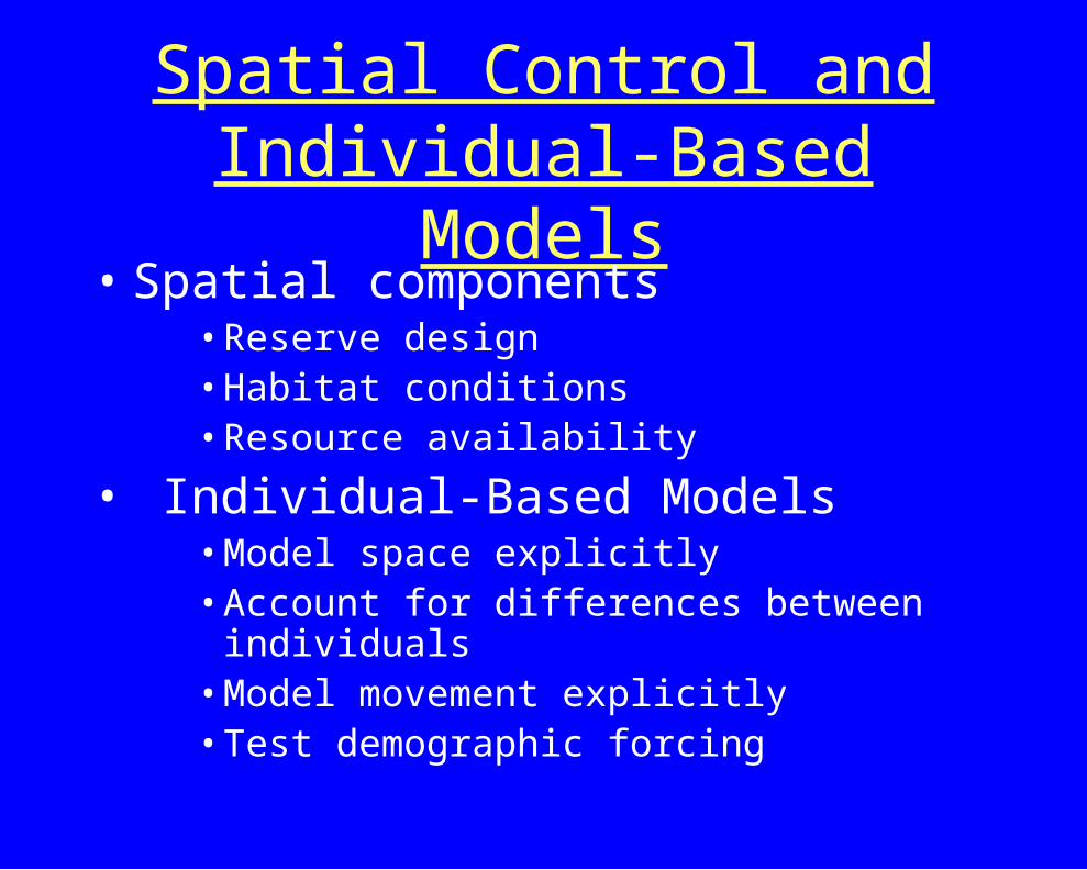
Spatial Control and Individual-Based Models

• Spatial components• Reserve design• Habitat conditions• Resource availability

• Individual-Based Models• Model space explicitly• Account for differences between individuals• Model movement explicitly• Test demographic forcing

American Black Bear (Ursus americanus)

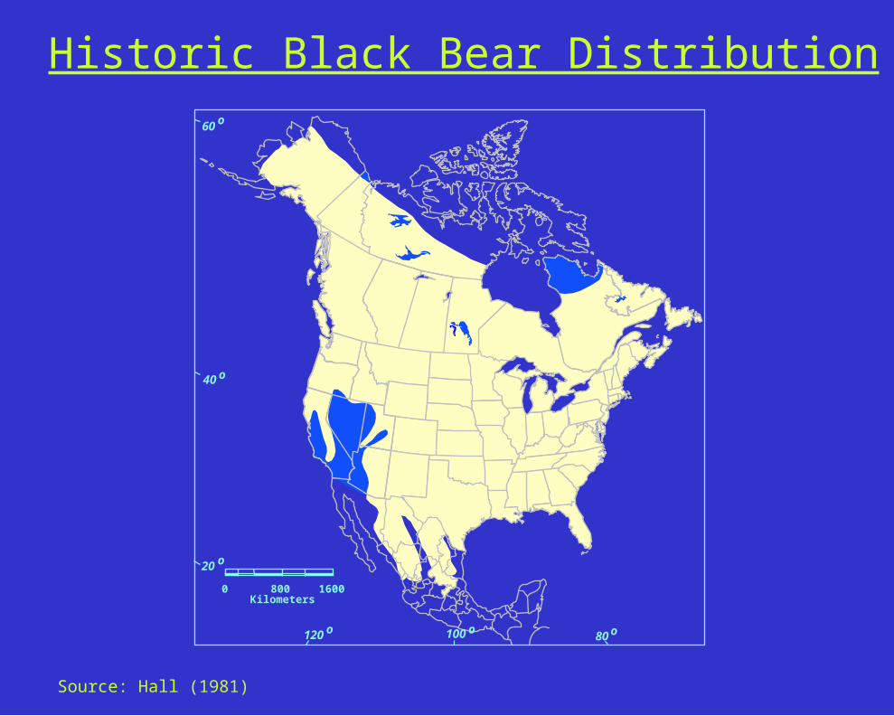
Historic Black Bear Distribution

Source: Hall (1981)

100 o

60 o

40 o

o

120 o 80 o

20

16000 800Kilometers

100 o

60 o

40 o

o

120 o 80 o

20

0 800Kilometers

1600

Current Black Bear Distribution

Source: Pelton and van Manen (1994)

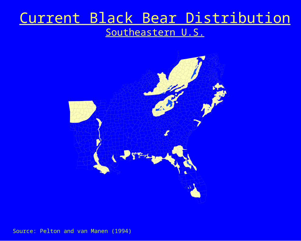
Current Black Bear DistributionSoutheastern U.S.

Source: Pelton and van Manen (1994)

Model Description

• Individual-Based• Time

• Daily time step• Length of run is user defined

• Area• 450m x 450m Cells• 279 Km x 175.5 Km (effective area is smaller)

• Allows for variation in various spatial components.• Sanctuaries• Park and forest boundaries

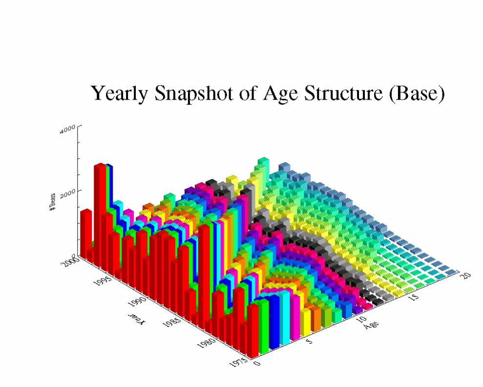
State Variables

• Age• Sex• Location• Denning • Estrus• Mating Status• Cubs

Flow DiagramInitialization

Set Mast Values? Mast Functions Yes

No

Movement

Update Food

Mortality

Update Indices

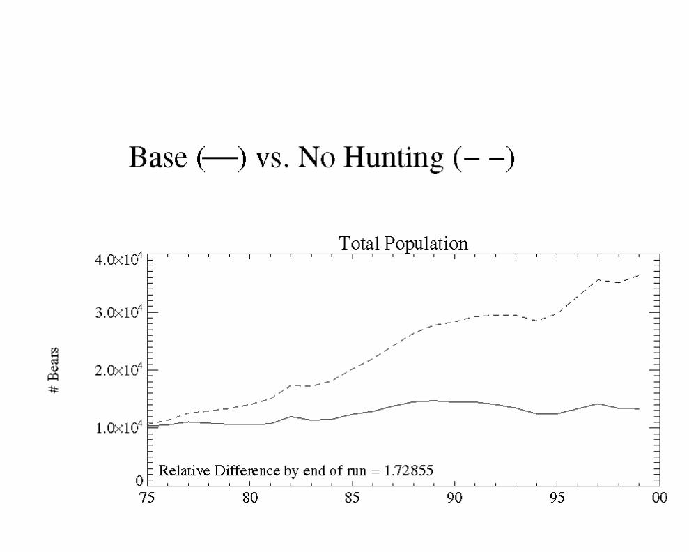
Harvesting

• Tennessee Season• Dec. 1- Dec. 14• No cubs or females with cubs.

• North Carolina Season• Oct.14 - Nov. 21 and Dec. 14 - Dec. 31• No cubs or females with cubs.

• No harvesting in GSMNP or bear sanctuaries.• One bear limit per calendar year

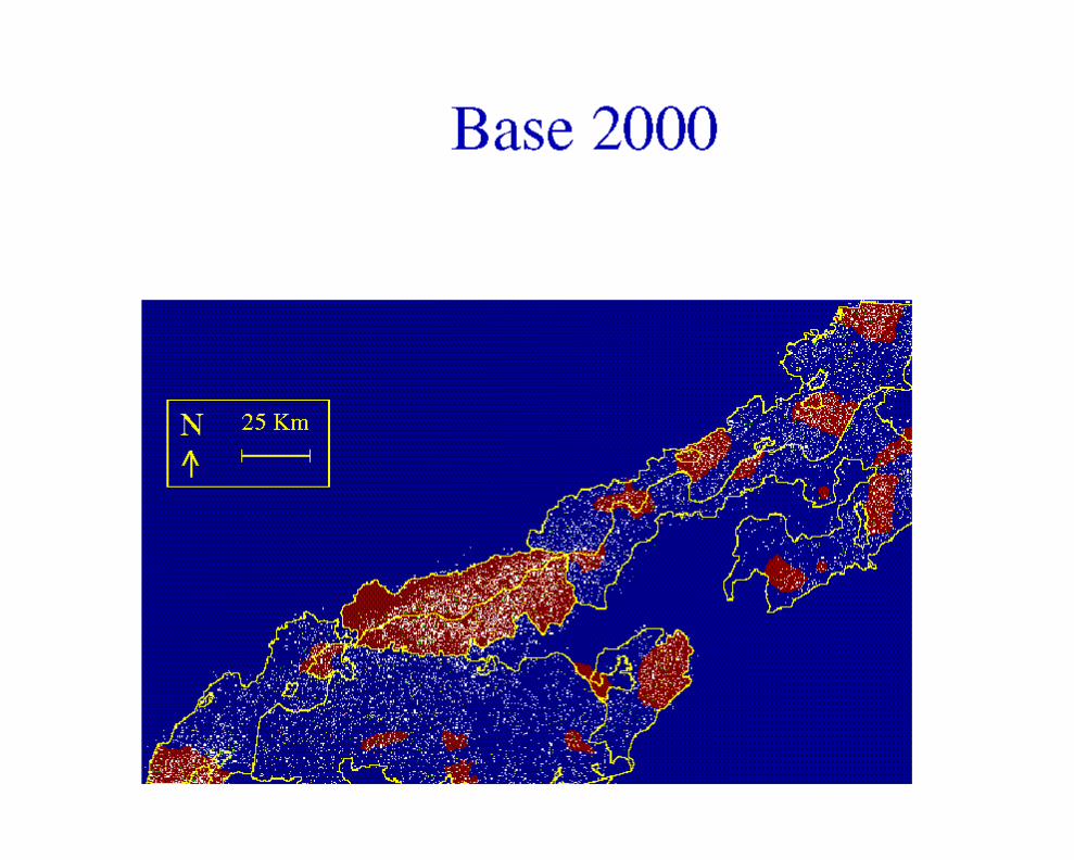
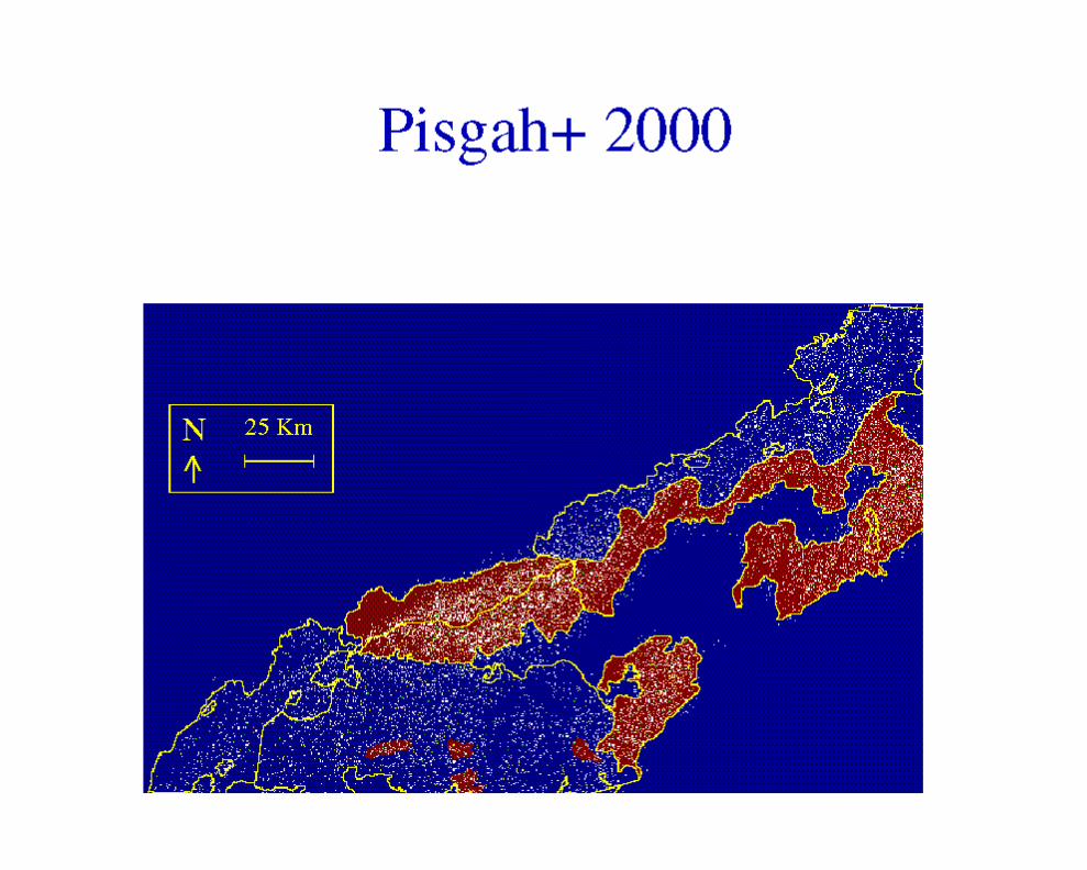
Variation in Spatial layout of Sanctuaries

• Nantahala• All of Nantahala National Forest is a sanctuary.• Aside from GSMNP, there are no other sanctuaries.

• Pisgah+• All of Pisgah National Forest is a sanctuary plus the present

sanctuaries in Nantahala.• Aside from GSMNP, there are no other sanctuaries.

• Each has approximately the same sanctuary area.

Spatial Control of Antibiotic Resistance • Assumption: Limitations on the application of

certain antibiotics can be viewed in a spatial context which, if effectively implemented, could extend the time period of utility of a particular antibiotic treatment.

• Question: Under what circumstances would a spatial control policy be preferable to a policy of uniform spatial rotation or a policy of local choice with no overall spatial management?

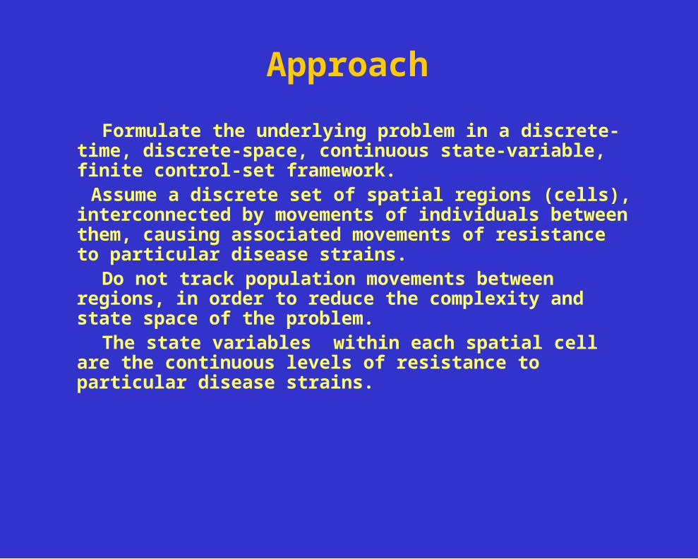
Approach

Formulate the underlying problem in a discrete-time, discrete-space, continuous state-variable, finite control-set framework.

Assume a discrete set of spatial regions (cells), interconnected by movements of individuals between them, causing associated movements of resistance to particular disease strains.

Do not track population movements between regions, in order to reduce the complexity and state space of the problem.

The state variables within each spatial cell are the continuous levels of resistance to particular disease strains.

Intercropping and Pathogen Dispersion • Assumption: There are two crop varieties, one of which is

more resistant to a pathogen but which has an associated higher cost or lower yield than the crop with lower resistance.

• Question: How might we analyze the spread of the pathogen linked to the growth of the crop and produce optimal spatial planting patterns which maximize yield, or minimize cost.

• Approach: Develop a general theory for boundary-control of reaction-diffusion type equations linked to ordinary differential equations for local crop growth.

vpcKvvr

dtdv

upcKuur

dtdu

pvpcupcpp xxt

2

2

2

1

1

1

22111

)1(

)1(

d

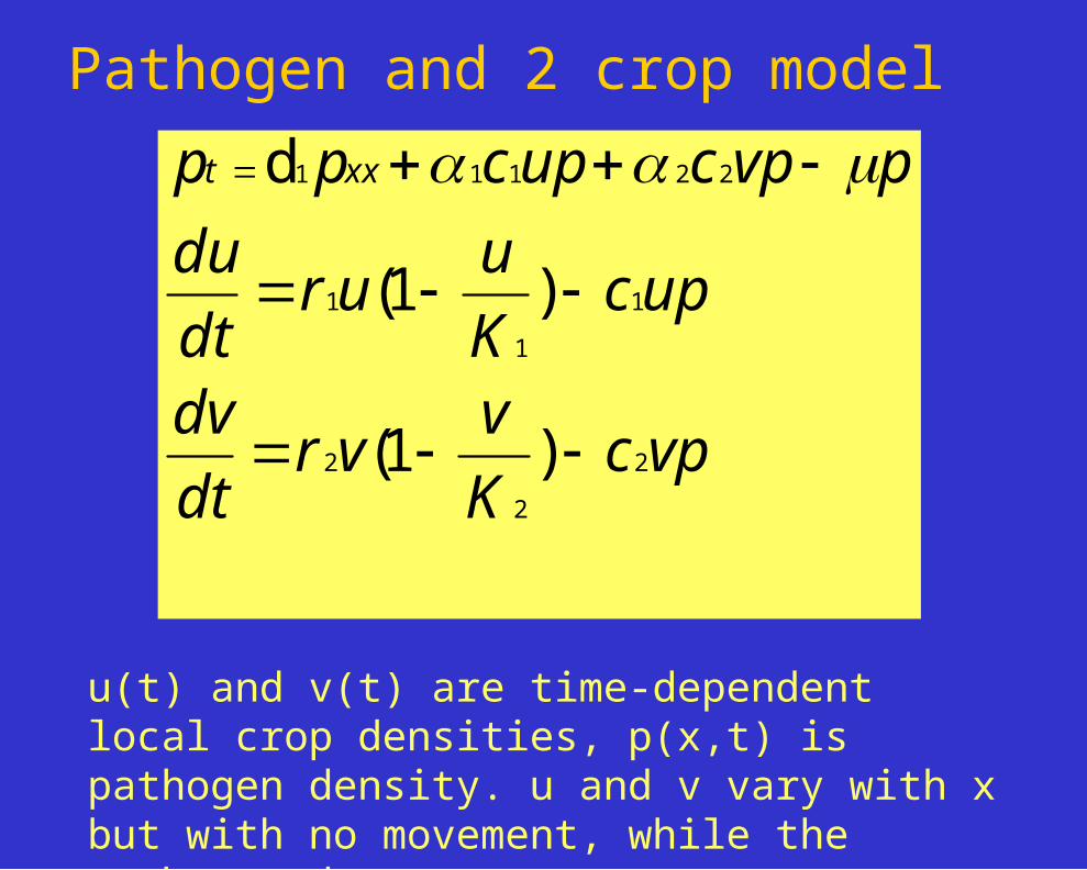
Pathogen and 2 crop model

u(t) and v(t) are time-dependent local crop densities, p(x,t) is pathogen density. u and v vary with x but with no movement, while the pathogen does move.

dxTxvAuAuJ )],)([(max)(1

0

210

Objective function is:

And choose u0(x) + vo(x) < K the maximum initial planting density. Assume Dirichlet boundary conditions for the pathogen, some initial pathogen distribution, and assume the spatial domain is [0,1]. Then with appropriate assumptions it is possible to develop optimal solutions.

We are also working on spatial control for integro-difference equations models of population spread.

Take-Home Messages• Realistic modeling of natural systems requires multiple linked

approaches – multimodeling - and new methods are needed to develop and analyze these.

• Much of applied ecology deals with problems of spatial control – what to do, where to do it, when to do it, and how to monitor it – and these problems are not easily solved, opening up many new, fascinating problems in applied mathematics and computational science.

Acknowledgements

• USGS Biological Resources Division• National Science Foundation• UT Center for Information Technology

Research• UT Scalable Intra-Campus Network Grid