An equilibrium model for spot and forward pricesof commoditiesI

Michail Anthropelosa,1, Michael Kupperb,2, Antonis Papapantoleonc,3

ABSTRACT

We consider a market model that consists of financial investors andproducers of a commodity. Producers optionally store some produc-tion for future sale and go short on forward contracts to hedge theuncertainty of the future commodity price. Financial investors take po-sitions in these contracts in order to diversify their portfolios. The spotand forward equilibrium commodity prices are endogenously derivedas the outcome of the interaction between producers and investors. As-suming that both are utility maximizers, we first prove the existence ofan equilibrium in an abstract setting. Then, in a framework where theconsumers’ demand and the exogenously priced financial market arecorrelated, we provide semi-explicit expressions for the equilibriumprices and analyze their dependence on the model parameters. Themodel can explain why increased investors’ participation in forwardcommodity markets and higher correlation between the commodityand the stock market could result in higher spot prices and lower for-ward premia.

KEYWORDS: Commodities, equilibrium, spot and forward prices, for-ward premium, stock and commodity market correlation.

AUTHORS INFOa University of Piraeus, 80 Karaoli and Dim-itriou Str., 18534 Piraeus, Greeceb University of Konstanz, Universitätstraße10, 78464 Konstanzc Institute of Mathematics, TU Berlin, Straßedes 17. Juni 136, 10623 Berlin, Germany1 anthropel@unipi.gr2 kupper@uni-konstanz.de3 papapan@math.tu-berlin.de

PAPER INFO

AMS CLASSIFICATION: 91B50, 90B05

JEL CLASSIFICATION: Q02, G13, G11, C62

1. Introduction

Since the early 2000s, the futures and forward contracts written on commodities have been awidely popular investment asset class for many financial institutions. As indicatively reportedin [17], the value of index-related futures’ holdings in commodities grew from $15 billion in2003 to more than $200 billion in 2008.1 This significant inflow of funds has coincided, up to

IWe are grateful to Ulrich Horst, Kasper Larsen, Dilip Madan, Christoph Mainberger, Steven Shreve, Ronnie Sir-car and Stathis Tompaidis for helpful discussions and suggestions. We thank two anonymous referees for theirvaluable comments that have significantly improved the paper. We also thank seminar participants at CarnegieMellon University, the 11th German Probability and Statistics Days in Ulm, the Workshop in New Directionsin Financial Mathematics and Mathematical Economics in Banff, the Workshop on Stochastic Methods in Fi-nance and Physics in Crete, the International Conference in Advanced Finance and Stochastics in Moscow, theConference on Frontiers in Financial Mathematics in Dublin, the Conference on Stochastics of Environmentaland Financial Economics in Oslo, the 8th World Congress of the Bachelier Finance Society in Brussels, and theSeminar in Stochastic Analysis and Stochastic Finance in Berlin for their comments. Financial support from theIKYDA project “Stochastic Analysis in Finance and Physics” is gratefully acknowledged.

1According to a recent estimation by Barclays Capital, the total commodity-linked assets were around $325 billionat the end of June 2014 (see Barclays Investment Bank 2014 and [33]).

1

arX

iv:1

502.

0067

4v3

[q-

fin.

EC

] 2

1 Ja

n 20

17

2008, with a steep increase in the spot and futures prices of the majority of commodities, espe-cially the ones included in popular commodity indices. The comovement of amounts invested incommodity-linked securities and the prices of the associated commodities continued even duringthe prices’ bust in 2008 and their recovery which started in 2009; see e.g. the empirical studiespresented in Singleton [57], Tang and Xiong [60] and Buyuksahin and Robe [10].2 Furthermore,several statistical studies have found that the correlation between commodity prices and the stockmarket has grown during the last years. As an example, [10] argues that the correlation of theU.S. stock market (weekly) returns and the returns of the GSCI commodity indices varies from-38% to 40% depending on the period, and stays positive and away from zero after 2009; fur-ther statistical evidence on the increased correlation are given in [60], [57] and in Singleton andThorp [56]. Therefore, the investment strategies of financial institutions on stock and commoditymarkets should be considered in the same optimization problem and not independently.

The booms and busts of the prices of major commodities during the last decade has naturallycaptured the interest of the academic community. The main question addressed is whether thebehavior of commodities’ prices is caused by the (enhanced by the financialization) positions ofspeculators or by the fluctuations of fundamental economic factors (i.e. increased demand andweakend supply).3 Even though there exist several empirical studies, the theoretical approachesthat link spot and forward prices of commodities with the rest of the investment assets are scarce.

The main goal of this paper, is to establish an equilibrium model that allows to endogenouslyderive both the spot and the forward price of a commodity, and is flexible and general enoughto include not only the randomness of the commodity demand and the commodity holders’storage option, but also risk averse agents and correlation between the stock and the commoditymarket. In our model, equilibrium commodity prices are formed as the outcome of the interactionbetween market participants, and simultaneously clear out the spot and the forward market.The forces that lead to the market equilibrium are the producers’ goal to maximize their spotrevenues and optimally hedge the risk of the future commodity price, and the investors’ goalto achieve an optimal portfolio strategy that, besides the stock market, includes also a positionin the commodity’s forward contracts. The model offers new insights on how specific modelinputs, such as the agents’ risk aversion, the correlation of the stock and commodity market andthe uncertainty of the future commodity price, influence the equilibrium prices and the relatedrisk premia.

1.1. Model description

We consider a model of two points in time: the initial one and a given (short-term) future horizonT . We assume that the main market participants are the representative agents of the commodity’s

2In [57], it is shown that investors’ index positions in crude oil are highly correlated with crude oil prices, while[10] provides statistical evidence which indicates that the excess speculation in U.S. Commodity Futures Marketsincreased from 11% in 2000 to more than 40% in 2008. In theoretical terms, this correlation affects heavily theagents’ optimization problems (see among others [11]).

3The opinion that speculative forces are the main reason for the booms and busts of commodity prices (especially inoil and gas markets) is supported by the empirical studies in [33, 57, 60], while [10, 32, 52, 59] provide statisticaltests that are in favor of the fundamental economic reasoning (see also [39, 44]). For a more detailed literaturesurvey on this debate, we refer the reader to [33] and [52].

2

holders/suppliers and the financial investors/speculators, who shall hereafter be called produc-ers4 and investors5 respectively.

The producers’ source of income are the revenues from spot and future sales. While the com-modity spot price could be determined by the spot commodity demand function, the future priceis subject to demand shocks. Assuming that producers are risk averse, their goal is not only tomaximize their spot revenues, but also to reduce their risk exposure to the future commodityprice by maximizing their expected utility.6 If the production schedule at the initial and futuretime is a predetermined pair of units, producers have two decisions to make: what amount of theproduction to supply in the spot market (inventory management) and what position to take in theforward contract (hedging strategy). Provided they know the demand function of the commod-ity’s consumers at the initial time, they can determine the commodity spot price by choosing theamount of the inventory they will hold up to the terminal time. However, random demand shocksat time T will shift the whole demand function to lower or higher levels (for instance, in Section4 we suppose that the random shift of the demand function is driven by a vector of stochasticmarket factors). Producers hedge the risk which stems from the future time demand function bytaking a short position in forward contracts written on the same commodity and with maturityequal to T . The fact that the inventory will also be sold at time T makes the forward hedgingposition even more important for the producers.7

The producers’ hedging demand is covered by financial investors, who take the opposite po-sition in the forward commodity contracts and thus share some of the future price uncertaintyrisk, possibly against a premium. They invest optimally in an exogenously priced stock market8

and are willing to take the future commodity price risk in order to better diversify their portfolio.Indeed, as mentioned above, the correlation between commodity and stock market indices hasbeen shown to be away from zero. This correlation could be incorporated in a model where thestock market price is driven by the same stochastic factors that drive the evolution of the com-modity demand function. Given this correlation, the optimal investment strategy in the stock andthe commodity market should be considered in the same optimization problem. As in the pro-ducers’ side, we assume that the investors are represented by an agent who is a utility maximizer

4We refer to the commodity sellers as producers by following the related literature (see e.g. [1, 6, 52]). Some authorsimpose that the representative agent of the supply side is the commodity refiners or storage managers who holdthe production and in some cases control its supply in the market (see for instance [24, 49]). In our model, theproduction schedule is a given input and the spot revenues of the producers come only from the commodity sales,thus our findings apply directly in case the refiners are the ones that distribute the commodity in the market.

5As highlighted in [45], it is rather difficult to identify whether the long position in the commodity forward contractsis taken by investors who just want to diversify or by speculators who invest based on specific predictions aboutthe move of commodity prices. As a matter of fact, the holders of a long position in the forward contract can alsobe called insurers, since they undertake some of the producers’ risk. Without attempting to enter in this debate,we will call the producers’ counterparties in the forward contract investors.

6The massive use of derivatives by natural gas and crude oil producers presented in Table 1 of [1] is a clear evidencethat commodity producers are indeed risk averse regarding their future revenues.

7The significance of the inventory policy in the spot and forward price fluctuations has been highlighted by manyauthors, see e.g. [31, 44, 51, 57] for detailed discussions and statistical evidence, especially in the popular exampleof crude oil prices.

8Here, exogenously means that investors in the commodity forward contract are price takers in the stock market.This implies that the volume in the commodity forward contracts is not so large to influence the price of the stockmarket, an assumption that is supported by the corresponding market volumes.

3

and whose investment choices are the (possibly dynamic) trading strategy in the stock marketand the position in the forward commodity contract.

The optimization choices of both producers and investors clearly depend on the forward com-modity price. We define as equilibrium forward price the price that clears the forward marketand at which both participants’ expected utilities are maximized. Given the forward price, theproducers optimally choose the inventory policy, which in turn gives the initial commodity sup-ply and thus determines the spot price through the initial demand function of the consumers.Therefore, by deriving the equilibrium forward commodity price, the equilibrium spot price aswell as the producers’ optimal inventory policy are also endogenously derived in our model.

1.2. Findings and contributions

The main mathematical result of this work is to prove, under CARA preferences and upon someminor technical assumptions, that equilibrium spot and forward commodity prices exist. In thisproof, we use standard duality arguments to show that both producers’ and investors’ optimiza-tion problems are well-defined and admit finite solutions. The existence of the forward commod-ity equilibrium price is first proved for every fixed producers’ storage choice. Then, we show thatthis equilibrium is stable with respect to the storage choice, which in turn guarantees the exis-tence of the commodity market equilibrium. In fact, this stability result is interesting in its ownright, since it shows that the market clearing is stable with respect to any control variable whichbelongs to a closed set of real numbers.

The constructive nature of the aforementioned proof allows us to derive implicit formulasfor spot and forward prices, which can be used to investigate how the main model parametersinfluence the commodity market. We illustrate this using two examples with factors driven byLévy processes; first a Brownian motion and then a jump-diffusion process. The main results aregiven below.

Focusing first on the equilibrium spot price, our results imply it is monotonic with respect tothe agents’ risk aversion coefficient; it is increasing for producers and decreasing for investors(see Figures 5.1 and 5.2). When producers are more concerned about the commodity futureprice uncertainty, they increase their position in the forward contract and hence lock the sellingprice at the terminal time. As long as the hedging position is counterpartied by the investors,high risk averse producers can increase their certain revenues today and at the same time hedgetheir future price risk. What is very important in this monotonicity is the correlation between thestock market and the demand random shocks. As it is illustrated in Section 5, when correlationis away from zero, the equilibrium spot price is pushed upwards. This is mainly because highercorrelation means that investors are able to better hedge their risk exposure in the commoditymarket by adjusting their investments in the stock market. Hence, they are willing to receive alower forward premium, thus making hedging cheaper for the producers. In particular, when theinvestors are more risk averse, they reduce their share in the future commodity price risk; thus,producers cannot hedge their future price risk which forces them to increase their supply in thespot market. Therefore, the spot price is a decreasing function of investors’ risk aversion (all elseequal). Also, it follows that the producers’ ability to hedge their risk tends to increase the spotequilibrium prices. Moreover, our model yields that the existence of a forward contract in thecommodity market stabilizes spot prices when there is scarcity of the commodity at the terminal

4

time; in particular, the presence of forward contracts increases the current spot and decreases theexpected future spot price of the commodity.

The monotonicity of the spot price with respect to risk aversions could also be used to explainhow the participation of investors in the commodity forward markets could result in an increaseof spot commodity prices. Indeed, under CARA preferences the more investors participate in themarket, the higher the aggregate risk tolerance becomes or, equivalently, the lower the represen-tative risk aversion’ coefficient becomes (see, among others, Wilson [61]). As discussed above,this implies higher spot commodity price, a result that is consistent with the observed marketdata (see e.g. [10] and Henderson et al. [33]). Similarly, we verify that more producers (of thesame total production) implies lower spot price.

Besides equilibrium commodity spot prices, our model allows to endogenously derive quanti-ties that characterize the two major, and not mutually exclusive, theories of forward commoditymarkets: the theory of storage and the theory of normal backwardation. Based on the ideas intro-duced in Kaldor [40], Working [62] and Brennan [9], the theory of storage states that the holdersof the commodity inventories get an implicit benefit, called convenience yield, which implies thevalue of the spot commodity consumption. This yield can be approximated by the difference be-tween the spot and the forward price minus the cost of storage. Our equilibrium model verifiesthat the convenience yield is increasing with respect to the producers’ risk aversion, meaningthat the more sensitive about the risk the producers are, the more commodity forward units theyhedge depressing the forward price (see Figure 5.6 for the Brownian motion example). A similarincreasing relation holds for the investors (these relations, in particular, generalize the resultsof Proposition 1 in Acharya et al. [1]). However, the convenience yield is not always mono-tonic with respect to the correlation coefficient. As discussed in Section 4, there are two effectsof opposing direction on the convenience yield, one coming from the decrease of the effectiveinvestors’ risk aversion and other from the corresponding increase on the spot price. The totaleffect mainly depends on the level of the agents’ risk aversions and the (uneven) productionlevels at initial and terminal time (see Figures 5.6 and 5.7).

On the other hand, the theory of normal backwardation (see the seminal works by Keynes [43]and Hicks [34]), states that there is a positive premium required by the investors in order to sat-isfy the producers’ hedging demand in forward contracts. This premium, usually called forwardor insurance premium, is given as the percentage difference between the expected commodityprice at maturity and its forward price. As expected, this premium is increasing (decreasing)with respect to investors’ (producers’) risk aversion.

In contrast to the existing literature, our model includes as an input the correlation between thestock market and the commodity demand shock. Several empirical studies have shown that thiscorrelation is indeed non-zero and, as our results demonstrate, it does influence the equilibriumprices heavily. In particular, as it is shown in Section 5, the effective investors’ risk aversioncoefficient is decreasing in the presence of non-zero correlation. This simply reflects the factthat higher correlation means better hedging of the forward contract position by trading in thestock market (provided there are no short-selling constraints on the investors’ trading strategies).Hence, non-zero correlation has in principle the same effect on the equilibrium as a decrease inthe investors’ risk aversion (see Figures 5.1, 5.2 and 5.5). For instance, higher correlation (inabsolute values) means higher spot commodity price, a result that is also consistent with theobserved market data (see e.g. [60]). A similar effect is caused by an increased variance of the

5

demand shock, which can be due to the presence of jumps (see Figure 5.5).

1.3. Relation with the existing literature

Equilibrium pricing models in markets that consist of utility maximizing agents have been re-cently addressed by a number of authors in mathematical finance; see, among others, Anthro-pelos and Žitkovic [4], Barrieu and El Karoui [7], Cheridito et al. [15], Filipovic and Kupper[25], Horst and Müller [37] and Karatzas et al. [42]. The results in this literature however do notcover the case of commodity forward contracts, not only because a commodity has a consump-tion value which is reflected by the consumers’ demand function, but also due to the producers’specific storage choice. To the best of our knowledge, this paper is the first to apply a utility max-imization criterion for spot and forward equilibrium prices of commodities, while consideringalso the existence of a correlated stock market.

Theoretical studies of the equilibrium relationship between spot and forward commodityprices go back to Anderson and Danthine [3], Stoll [58] and Hirshleifer [35, 36]. The resultsof these seminal works are limited regarding the agents’ risk preferences, which are assumedto be mean-variance, while recent extensions of this setting have followed different approachesthan ours. For instance in Baker [6], mean-variance optimization problems are imposed in adiscrete time dynamic model, where investors are the ones that have the storage option and theconsumers (the households) get utility from consumption and the wealth (numéraire units). InRoutledge et al. [51] and Pirrong [49], investors are assumed to be risk neutral and without ac-cess to other financial markets, while forward prices are simply the expectations of future spotprices. The interaction between the optimal storage and the investors’ optimal position in theforward contract and its effect to spot and forward equilibrium prices are also studied in Ekelandet al. [24]. However, in contrast to our model the investors trade only in forward contracts, whilethe preferences are mean-variance, which means that they are not monotonic with respect tofutures revenues. More recently, endogenous commodity supply under asymmetric informationand limited participation has been developed in Leclercq and Praz [48]. Static mean-variancemodels have been also studied and statistically tested in Acharya et al. [1] and Gorton et al.[30], however neither the investors nor the producers trade in any other market outside of thecommodity market9. Hence, their theoretical results cover only a very special case of our model,namely, when the stock and the commodity market are uncorrelated and the demand randomshift is normally distributed.10

The main novelties of our approach compared to the related literature are the consideration ofan exogenous stock market available in the investors’ trading set, the risk aversion of the agents’preferences and the much richer family of processes that model the market factors.11 Indeed, as

9In [1] investors are assumed risk neutral, but the imposed capital constraints eventually lead to a mean-varianceoptimization criterion, while in [30] there is a random supply shock at the terminal time, which however does notchange the general idea of the equilibrium setting.

10Continuous time dynamic models with random demand shocks and exogenously given spot prices have beendeveloped in [8] and [13].

11The seminal works [58] and [35] also include a correlated risky asset in the investors’ set of strategies, forming anequilibrium framework. However, our results are more general regarding not only the utility preferences and thestochasticity of the market model, but also the set of investors’ trading strategies.

6

has already been discussed, both the correlation between the stock and commodity market andthe jump component do influence the equilibrium prices.

This paper is structured as follows: Section 2 sets up the general framework for our equilib-rium model. The well-posedness of the agents’ optimization problems and the existence of anequilibrium are proved in Section 3. Section 4 studies a model with continuous trading underLévy dynamics, where semi-explicit formulas for equilibrium quantities are derived and dis-cussed. Finally, Section 5 focuses on two examples that permit the illustration and a furthereconomic interpretation of the results. Technical proofs of Section 5 are placed in Appendix A.

2. A general framework for commodity prices

We start by describing a general modeling framework where the interaction of market partici-pants determines the spot and forward prices of commodities. The model consists of a pair ofrepresentative agents12: the producers produce the commodity, supply part of the productionat the spot market and store the rest, while they hedge their exposure to price fluctuations us-ing forward contracts on the commodity. The investors invest in financial markets and, in orderto diversify their portfolio, they also invest in the commodities forward market. Moreover, themodel includes consumers who consume the commodity at the spot market. The goal is to de-termine the price of the commodity that makes the forward market clear out, assuming that bothproducers and investors are utility maximizers.

More specifically, the producers produce π0 units of the commodity at the initial time 0 andπT units at the terminal time T ; both π0 and πT are assumed to be deterministic13. They offerπ0 − α units at the spot market at time 0 and store the rest for time T . Furthermore, they hedgetheir exposure by investing in the forward market. Therefore, their position at time T is

w(α, hp) = P0(π0 − α)(1 +R) + PT (πT + α(1− ε)) + hp(PT − F ), (2.1)

where P0 and PT denote the spot price at times 0 and T respectively, R the discretely com-pounded interest rate, ε ∈ [0, 1] the cost of storage considered as percentage of the stored units14,F the forward price and hp the amount of forward contracts held by the producers. A positivehp indicates a long position in the forward contract, while a negative hp amounts to a short one.The producers’ utility is assumed to be exponential, henceforth their preferences are describedby

Up(v) = − 1

γplogE

[e−γpv

], (2.2)

where γp > 0. As in Anderson and Danthine [2, 3], their problem is to find an optimal storagestrategy α ∈ [0, π0] and an optimal hedging strategy hp ∈ R that maximize the utility of their

12The representation by a unique agent is widely used in this literature, see [1, 8, 24, 30, 57] among others.13This assumption means that the producers control the supply of their commodity only through the inventory man-

agement and not by changing their production plans, which can be prohibitively costly in the short-term (see alsothe related comment in [1]).

14The representation of the storage cost as percentage is common in the related literature, see e.g. [1] and [30]. Theconstant cost rate ε is usually referred to as the depreciation rate.

7

position (2.1). Therefore, their utility maximization problem is

Πp := supα∈[0,π0], hp∈R

Up(w(α, hp)

). (2.3)

The spot price of the commodity is the price at which the consumers’ demand equals theproducers’ supply. The consumers’ demand at the initial time is given by a strictly decreasingand linear function15

ψ0(x) = µ−mx, (2.4)

where µ ∈ R and m ∈ R+, while x denotes the price. The parameter m is a measure of theelasticity of demand for the commodity. The demand at the terminal time is random and dependson the factors driving the commodities market, which are incorporated in a random variable X .The demand function at the terminal time is of the form

ψT (x) = ψ0(x) +X. (2.5)

In other words, we assume that the shape and the elasticity of the demand function remain thesame, however there is a random shift16 acting on it. This shift may be, for example, the resultof an increase or decrease in the prices of the competitive commodities, of fluctuations in adominated currency, or of an exogenous increase in the demand for every price level. Since thedemand function is linear, the inverse demand function is also linear and equals

φ0(y) =µ− ym

and φT (y) =µ+X − y

m. (2.6)

Henceforth, if the producers store α units at the initial time, the spot price of the commodity,determined by the equilibrium condition between demand and supply, equals

P0 = φ0(π0 − α) = φ0(π0) +α

m, (2.7)

while the commodity spot price at the terminal time is

PT = φT(πT + α(1− ε)

)= φ0(πT )− α(1− ε)

m+X

m. (2.8)

The producers control the spot price by choosing the inventory policy. By storing more com-modity units they increase the spot price, but they also increase their exposure to the variationof the future spot price since the stored units will be supplied at the next time period.

The investors take a position hs in the forward contract and invest in an exogenously17 pricedfinancial market. Their position at time T equals

w(G, hs) = hs(PT − F ) +G, (2.9)

15The linearity of the demand function is imposed to facilitate the analysis. The limitation of this assumption doesnot exclude from our study the main characteristics of the demand, namely its elasticity and its random natureat terminal time. Let us also mention, that for a short time horizon a first order approximation of the demandfunction should suffice (see also the related discussion in [1, 24]).

16A similar random shift has already been used in the literature, see for instance [49].17In other words, the investors are price-takers when they invest in the financial market.

8

for G ∈ G, where G is a set of random variables that models discounted trading outcomes at-tainable with zero initial wealth. This general formulation allows to consider different scenariossimultaneously.

Example 2.1. The simplest scenario is G = 0, whence the investors can only invest in theforward contract. Another scenario is to consider an asset price process S and denote byG(θ) =∫ ·

0 θudSu the gains process for a trading strategy θ. In that case, the set of trading outcomes G isgiven by

G = GT (θ) : θ ∈ Θ,

for a set Θ of admissible, self-financing trading strategies. Transaction costs can be easily incor-porated as well by setting

G = GT (θ)− k(θ) : θ ∈ Θ,

where k : Θ→ R is a concave function. ♦

We assume that the investors’ utility is also exponential with γs > 0, that is, their preferencesare described by

Us(v) = − 1

γslogE

[e−γsv

], (2.10)

therefore their utility maximization problem reads as

Πs := suphs∈R, G∈G

Us(hs(PT − F ) +G

). (2.11)

The maximization problem of both participants depends on the forward price F . This price isdetermined by the equilibrium in the forward market, which is defined below.

Definition 2.2. A triplet (α, h, F ) is called an equilibrium if it satisfies the following conditions:

• Market clearing: the forward market clears out in the sense that

h := hp(F ) = −hs(F ). (2.12)

• Optimality: the pair (α, h) is optimal for the producers’ problem Πp and h is optimal forthe investors’ problem Πs.

The price F = F (α) is called the equilibrium commodity forward price at maturity T . Theinduced price P0 := P0(α) derived by (2.7) is called the equilibrium commodity spot price at 0.

Remark 2.3. The utility maximization problems of both agents are equivalent to risk minimiza-tion problems relative to the entropic risk measure; see e.g. Barrieu and El Karoui [7]. The riskmeasure point of view is more natural for certain agents, such as a corporation managing its riskexposure.

9

3. Equilibrium in the general framework

The aim of this section is to show that an equilibrium exists in the general modeling frameworkdescribed above, under mild assumptions on the random variable X and the set of trading out-comes G. Let (Ω,F ,P) be a probability space where F = FT . In the sequel all equalities andinequalities between random variables are understood in the P-almost sure sense. The interiorand the boundary of a set K are denoted by K and ∂K, respectively, and the domain of afunction f by domf .

We denote the set of exponential moments of X by UX = u ∈ R : E[euX ] <∞ and definethe cumulant generating function of X by

κX(u) = logE[euX

], u ∈ UX . (3.1)

The following conditions will be used throughout this work:

(EM) 0 ∈ UX .

(COE) If ∂UX = ±∞ then the following limit holds:

limz→±∞

κX(z)

|z|= +∞.

The next lemma summarizes some useful properties of the cumulant generating function.

Lemma 3.1. The cumulant generating function κX is convex and lower semicontinuous.

Proof. Convexity follows directly from Hölder’s inequality; for p, q ∈ (0, 1) conjugate, we havethat

κX(pu+ qv) = logE[epuXeqvX

]≤ log

(E[euX ]

)p(E[evX ])q

= pκX(u) + qκX(v).

In order to show lower semicontinuity, consider a sequence un → u; then eunx is a sequence ofpositive functions. Applying Fatou’s lemma, we get

lim infun→u

κX(un) = lim infun→u

logE[eunX

]≥ logE

[lim infun→u

eunX]

= κX(u).

3.1. Producers’ optimization problem

The first step is to consider the producers’ optimization problem and show that it admits a maxi-mizer under mild assumptions. The producers’ position, using the spot market equilibrium con-

10

ditions (2.7) and (2.8), can be written as

w(α, hp) = P0(π0 − α)(1 +R) + PT (πT + α(1− ε)) + hp(PT − F )

(2.7)=

(2.8)

(φ0(π0) +

α

m

)(π0 − α)(1 +R)− hpF

+(πT + α(1− ε) + hp

)(φ0(πT )− α(1− ε)

m+X

m

)=: q(α, hp) + `(α, hp)X, (3.2)

where q is a quadratic function18 in α and hp of the form

q(α, hp) = −α2 1 +R+ (1− ε)2

m+ α

2(1 +R)π0 − 2(1− ε)πT − (R+ ε)µ

m

− αhp 1− εm− hp

(F − µ− πT

m

)+ πTφ0(πT ) + π0φ0(π0)(1 +R), (3.3)

while ` is a bilinear function in α and hp given by

`(α, hp) =α(1− ε) + hp + πT

m. (3.4)

Using the translation invariance of the exponential utility function, the producers’ utility takesthe form

Up(w(α, hp)

)= − 1

γplogE

[exp

(− γp

q(α, hp) + `(α, hp)X

)]= q(α, hp)− 1

γplogE

[exp

(− γp`(α, hp)X

)]= q(α, hp)− 1

γpκX(− γp`(α, hp)

), (3.5)

assuming that −γp`(α, hp) ∈ UX . In the sequel, we will work with the extended producers’utility Up(w(α, hp)) which is defined as follows:

Up(w(α, hp)

)=

Up(w(α, hp)

), if (α, hp) ∈ UX ,

−∞, otherwise,(3.6)

where UX =

(x1, x2) ∈ R2 : −γp`(x1, x2) ∈ UX

. The producers’ optimization problem (2.3)can then be written as follows

Πp = supα∈[0,π0]

suphp∈R

Up(w(α, hp)

)= sup

α∈[0,π0]suphp∈Rup(α, hp)− hpF = sup

α∈[0,π0]−u∗p(α, F ), (3.7)

18It follows directly from (3.2) (see also the associated formulas in subsection 5.1), that if the parameter µ is suf-ficiently small, then producers may have motive to discard the commodity, in the sense that the total optimalsupply is less than the total production, even if the demand function is deterministic. We can avoid such cases, byassuming that the parameter µ is sufficiently large. Note that µ could be considered as the consumers’ demandwhen the commodity has zero price, hence assuming large values for µ is a reasonable assumption.

11

where

up(α, hp) =

q(α, 0)− 1

γpκX(− γp`(α, hp)

)− hp`(α,−µ), if (α, hp) ∈ UX ,

−∞, otherwise,(3.8)

while u∗p(α, ·) denotes the conjugate function of up(α, ·), for every α ∈ [0, π0].

Proposition 3.2. Assume that conditions (EM) and (COE) hold. Then, for every F ∈ R thereexists a maximizer (α, hp) for the producers’ problem Πp such that (α, hp) ∈ UX .

Proof. The function Up(w(α, hp)) in (3.5) is upper semicontinuous, strictly concave in α andconcave in hp, since q is quadratic, ` is linear and κX is convex and lower semicontinuous inits arguments; see Lemma 3.1 and (3.3)–(3.4). Observe that α takes values in a bounded set.If the set UX is also bounded, then the existence of a maximizer follows by the concavity andthe upper semicontinuity of Up(w(a, hp)). Otherwise, if UX is unbounded, using Assumption(COE), the linearity of ` in α and that α belongs to a bounded set, we get that

limhp→±∞

infα∈[0,π0]

κX(− γp`(α, hp)

)|hp|

= +∞. (3.9)

Therefore, Up(w(α, hp)) is coercive in hp resulting in the existence of a maximizer. Finally, if(α, hp) does not belong to UX , then the utility of the producers is not maximized, see (3.6).

Corollary 3.3. Assume that conditions (EM) and (COE) hold. Then, the function up(α, ·) isconcave and upper semicontinuous for every α ∈ [0, π0]. In addition, it is coercive uniformly inα, that is

limhp→±∞

supα∈[0,π0]

up(α, hp)

|hp|= −∞. (3.10)

Remark 3.4. It follows from (3.3), that small production at time T raises the producers’ desireto store, even when the future demand function is deterministic. This occurs because a possiblescarcity of the commodity at time T would result in higher future spot prices, hence producerswould be better off storing some production and selling it at time T . On the other hand, higherfuture production decreases the optimal storage choice. Hence, the producers’ desire to balanceuneven productions is an important feature that influences the optimal storage choice.

3.2. Investors’ optimization problem

The second step is to analyze the structure and properties of the investors’ optimization problem.Although we cannot prove the existence of a maximizer at this level of generality, the results weobtain are sufficient to show the existence of an equilibrium in the next subsection.

Let Q be a probability measure on (Ω,F). The relative entropy H(Q|P) of Q with respect toP is defined by

H(Q|P) =

EQ[

ln(

dQdP)], if Q P,

+∞, otherwise.

12

Given α ∈ [0, π0], the spot price of the commodity PT = PT (α) is provided by (2.8). Definethe function

us(α, hs) := sup

G∈GUs(hsPT +G

), (3.11)

for a convex set G of FT -measurable random variables that contains 0. In order to prove theexistence of an equilibrium we will make use of the following assumption:

(USC) The function hs 7→ us(α, hs) is upper semicontinuous for every α ∈ [0, π0].

The function hs 7→ us(α, hs) is also concave for every α ∈ [0, π0], while the investors’ opti-

mization problem can be expressed as follows

Πs = suphs∈R

supG∈G

Us(hs(PT − F ) +G

)= sup

hs∈Rus(α, hs)− hsF . (3.12)

Throughout this section, we will also make use of the sets

MG :=Q P : H(Q|P) <∞ and EQ[G] ≤ 0 for all G ∈ G

and

QX :=Q P : EQ[|X|] <∞.

The financial market is free of arbitrage if MG 6= ∅. This is a sufficient condition, but notnecessary, since it also requires the entropy to be finite. In the sequel, we also need the existenceof at least one probability measure inMG that belongs to QX19. We state these requirements inthe following condition:

(NA) MG ∩QX 6= ∅.

Proposition 3.5. Assume that (NA) holds. Then, for each α ∈ [0, π0] there exists F = F (α) ∈R such that

lim suphs→±∞

us(α, hs)

|hs|< +∞, (3.13)

and−u∗s(α, F ) := sup

hs∈Rus(α, hs)− hsF < +∞. (3.14)

Proof. Fix Q ∈ MG ∩ QX . Using (NA) and (2.8) we get that PT = PT (α) ∈ L1(Q) for allα ∈ [0, π0]. According to Föllmer and Schied [26, Lemma 3.29], for each G ∈ G, hs ∈ R andn ∈ N it holds that

Us([hsPT +G] ∨ (−n)

)= − 1

γslogE

[exp

− γs

([hsPT +G] ∨ (−n)

)]≤ EQ

[(hsPT +G) ∨ (−n)

]+

1

γsH(Q|P). (3.15)

19As we will see later on, this assumption is needed in order to guarantee that the commodity spot price PT (α) ∈L1(Q) for at least one Q ∈ MG and α ∈ [0, π0], which eventually implies that the investors’ utility is boundedfrom above. In the market model of Section 4, this assumption implies, in particular, that the investor’s indiffer-ence price of the commodity is bounded from above; see also Remark 4.6.

13

Since (PT +G)+ ∈ L1(Q) and EQ[G] ≤ 0, monotone convergence implies that

us(α, hs) = sup

G∈G

− 1

γslogE

[exp

− γs(hsPT +G)

]≤ hsEQ[PT ] +

1

γsH(Q|P),

which yields (3.13). Finally, defining F := EQ[PT ] we obtain that

suphs∈R

us(α, h

s)− hsF≤ 1

γsH(Q|P) < +∞. (3.16)

3.3. Existence of equilibrium

We are now ready to show that under mild assumptions an equilibrium exists in the generalmodeling framework described in Section 2. Explicit, and easily verifiable, conditions for theuniqueness of the equilibrium are also provided. We start with some preparatory results fromconvex analysis before stating and proving the main theorem.

According to (3.7), the producers’ optimization problem is described by

Πp = supα∈[0,π0]

suphp∈R

up(α, hp)− hpF = − infα∈[0,π0]

infhp∈R

hpF − up(α, hp)

= supα∈[0,π0]

−u∗p(α, F ). (3.17)

Similarly, from (3.12) and (3.14) the investors’ optimization problem is described by

Πs = suphs∈R

us(α, hs)− hsF = −u∗s(α, F ). (3.18)

In the sequel we will make use of several results from convex analysis; we refer the reader toRockafellar [50] for a comprehensive introduction. We define the sup-convolution of up and usvia

u(α, h) := suphp+hs=h

up(α, hp) + us(α, hs) , (3.19)

and we know that its conjugate function satisfies

u∗(α, F ) = infh∈RhF − u(α, h) = u∗p(α, F ) + u∗s(α, F ); (3.20)

cf. [50, Theorem 16.4]. Moreover, it holds that

u(α, h) = infF∈RhF − u∗(α, F ) (3.21)

and we know that F belongs to the supergradient of u(α, h), denoted by ∂u(α, h), if the equality

u(α, h) = hF − u∗(α, F ) (3.22)

is satisfied; see [50, Theorem 23.5]

14

Theorem 3.6. Assume that conditions (EM), (COE), (USC) and (NA) hold, and suppose that

−γp`(π0, 0) ∈ UX . (3.23)

Then there exists an equilibrium (α, h, F ).

Remark 3.7 (Uniqueness). The equilibrium in Theorem 3.6 is not unique in general, since thesupergradient ∂u(α, 0) is not a singleton. However, if the functions hp 7→ up(α, h

p) and hs 7→us(α, h

s) are differentiable for all α ∈ [0, π0], then the equilibrium commodity forward priceis unique. Indeed, the proof of Theorem 3.6 yields that any equilibrium commodity forwardprice F satisfies F ∈ ∂u(α, 0) for the unique optimizer α ∈ [0, π0]. If up(α, ·) and us(α, ·) areboth differentiable then it follows, for instance from Lemma 1.6.5 in Cheridito [14], that u(α, ·)is differentiable at 0, in which case ∂u(α, 0) is a singleton. Moreover, if hp 7→ up(α, h

p) andhs 7→ us(α, h

s) are strictly concave, then also the optimal strategy h is unique. These conditionscan be easily verified in the examples; see Sections 4 and 5.

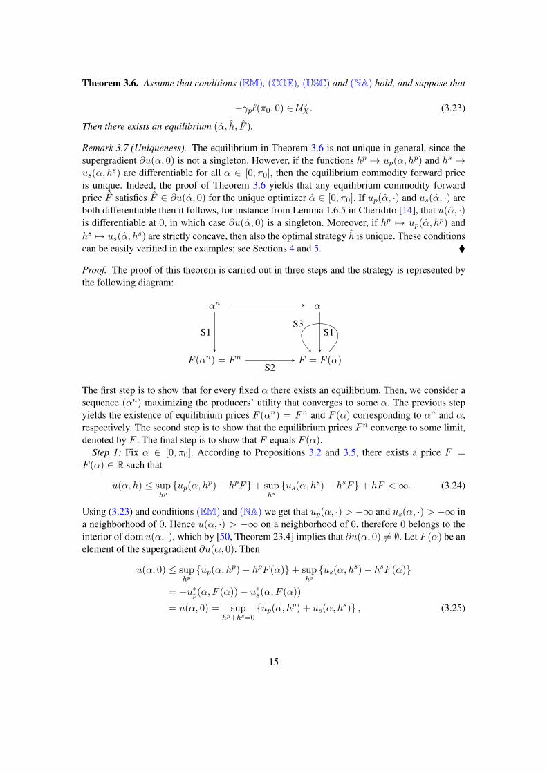
Proof. The proof of this theorem is carried out in three steps and the strategy is represented bythe following diagram:

αn α

F (αn) = Fn F = F (α)

S1

S2

S1S3

The first step is to show that for every fixed α there exists an equilibrium. Then, we consider asequence (αn) maximizing the producers’ utility that converges to some α. The previous stepyields the existence of equilibrium prices F (αn) = Fn and F (α) corresponding to αn and α,respectively. The second step is to show that the equilibrium prices Fn converge to some limit,denoted by F . The final step is to show that F equals F (α).

Step 1: Fix α ∈ [0, π0]. According to Propositions 3.2 and 3.5, there exists a price F =F (α) ∈ R such that

u(α, h) ≤ suphpup(α, hp)− hpF+ sup

hsus(α, hs)− hsF+ hF <∞. (3.24)

Using (3.23) and conditions (EM) and (NA) we get that up(α, ·) > −∞ and us(α, ·) > −∞ ina neighborhood of 0. Hence u(α, ·) > −∞ on a neighborhood of 0, therefore 0 belongs to theinterior of domu(α, ·), which by [50, Theorem 23.4] implies that ∂u(α, 0) 6= ∅. Let F (α) be anelement of the supergradient ∂u(α, 0). Then

u(α, 0) ≤ suphpup(α, hp)− hpF (α)+ sup

hsus(α, hs)− hsF (α)

= −u∗p(α, F (α))− u∗s(α, F (α))

= u(α, 0) = suphp+hs=0

up(α, hp) + us(α, hs) , (3.25)

15

where the second to last equality follows from (3.20) and (3.22) using that h = 0. By meansof Corollary 3.3 and Proposition 3.5 we deduce that the function h 7→ up(α, h) + us(α,−h)is concave and tends to −∞ as h → ±∞; see in particular (3.10) and (3.13). Therefore, thesupremum in (3.25) is attained for hp(α), hs(α) ∈ R with hp(α) + hs(α) = 0. Moreover, itfollows from (3.25) that

hp(α) = argmax up(hp, α)− hpF (α) and hs(α) = argmax us(hs, α)− hsF (α) .

In other words, for every fixed α ∈ [0, π0] there exists an equilibrium.Step 2: Consider an optimizing sequence (αn) for the producers’ utility converging to α, then

−u∗p(αn, Fn) −−−→n→∞

supα−u∗p(α, F (α)), (3.26)

where Fn = F (αn) is the sequence of equilibrium prices corresponding to αn. Let us nowprove that both the equilibrium prices Fn and the optimal strategies hn = hp(αn) = −hs(αn)are bounded; henceforth hn → h and Fn → F by possibly passing to a subsequence.

The upper semicontinuity of up, condition (USC) and the definition of the sup-convolutionyield that

lim supn→+∞

u(αn, 0) ≤ lim supn→+∞

up(αn, hn) + us(αn,−hn) ≤ up(α, h) + us(α,−h) ≤ u(α, 0),

which is finite by (3.24). Moreover, due to condition (3.23) there exists a neighborhood V of 0such that

infhp∈V

infn∈N

up(αn, hp) > −∞.

Hence, there exist constants c1 ∈ R and c2 > 0 such that

−u∗p(αn, Fn) = suphp∈R

up(αn, hp)− Fnhp ≥ c1 + c2|Fn|

and similarly−u∗s(αn, Fn) ≥ c1+c2|Fn|. Therefore, 2c1+2c2|Fn| ≤ supn∈N u(αn, 0) < +∞showing that (Fn) is bounded. Since

−u∗p(αn, Fn) = up(αn, hn)− hnFn,

it follows from Corollary 3.3 that (hn) is also bounded.Step 3: Finally, the goal is to identify F as the desired equilibrium price, that is, prove that

F = F (α). We start by showing that

u∗p(αn, Fn) −−−→

n→∞u∗p(α, F ). (3.27)

Indeed, by continuity of up(α, hp) in α we get that hpFn − up(αn, hp) → hpF − up(α, hp).Thus, by the definition of the conjugate u∗p(α, F ) = infhphpF − up(α, hp), it follows that

lim supn→∞

u∗p(αn, Fn) ≤ u∗p(α, F ).

16

Moreover, equilibrium prices belonging to the supergradient of u, ensures that

lim infn→∞

u∗p(αn, Fn) = lim inf

n→∞hnFn − up(αn, hn) ≥ hF − up(α, h) ≥ u∗p(α, F )

and thus lim infn→∞ u∗p(α

n, Fn) ≥ u∗p(α, F ). Hence (3.27) holds. The same argumentationimplies that u∗s(α

n, Fn)→ u∗s(α, F ).Next, we show that u(αn, 0)→ u(α, 0). On the one hand, there exists an h′ ∈ R such that

u(α, 0) = up(α, h′) + us(α,−h′) = lim

n→∞up(αn, h′) + us(α

n,−h′) ≤ lim infn→∞

u(αn, 0).

The first equality holds since the supremum is attained, the second follows from the continuityof up and us in α and the last one by (3.19). On the other hand, (hn) converging to h implies

lim supn→∞

u(αn, 0) = lim supn→∞

up(αn, hn) + us(αn,−hn) ≤ up(α, h) + us(α,−h) ≤ u(α, 0),

making use of the same argumentation for each equality as above.Summarizing, using the convergence of the sup-convolutions, (3.22), (3.20) and the conver-

gence of the conjugates, we arrive at

u(α, 0) = limn→∞

u(αn, 0) = limn→∞

−u∗p(αn, Fn)− u∗s(αn, Fn) = −u∗p(α, F )− u∗s(α, F ).

(3.28)In particular, the sup-convolution u(α, 0) is attained at hp(α) = h and hs(α) = −h ∈ R forwhich hp(α) + hs(α) = 0. Therefore, according to (3.26) and (3.28) the pair (α, hp(α)) andhs(α) are optimal trading strategies for the price F which satisfy the clearing condition. Hence(α, hp(α), F ) is an equilibrium.

4. A model with continuous trading and dependent markets

In this section, we consider a model where investors are allowed to trade continuously overtime in the financial market, while the dynamics of the financial and the commodity markets aredependent and driven by Lévy processes. The aim is to derive explicit representations for theoptimization problems of the producers and the investors.

Lévy processes have been used for modeling variables in finance, such as stocks or interestrates, whose return distributions exhibit fat tails and skew, because they can combine realisticfeatures with analytical tractability; see e.g. Carr et al. [12], Cont and Tankov [18], Eberlein [20]and Schoutens [54]. Gorton and Rouwenhorst [29] provide evidence that commodity futuresexhibit similar behavior. Using Lévy processes, we can easily combine diffusions with jumpprocesses, while different types of dependence structures can also be incorporated.

In the model considered in this section, the investors observe the evolution of the consumers’demand through time and adjust their trading strategy dynamically20. Moreover, the uncertainty20It is implicitly assumed that the investors’ investment choices are independent of their possible commodity con-

sumption policy. This assumption has been imposed in the majority of the related literature (cf. [1, 13, 24, 35]) andimplies that the consumers or corporations that use the commodity to produce other goods are only a small partof the investors’ side and their possible joint optimization problem is negligible when the investors are consideredas a whole.

17

in the evolution of the consumers’ demand and the evolution of the financial market are depen-dent processes which can exhibit ‘shocks’ (i.e. large jumps). The producers are trading in theforward market only at discrete time instances, associated with their production schedule21. Thissetting reflects real-world situations, in the sense that the arrival of certain news can affect boththe demand for a certain commodity as well as the financial market, these processes are observ-able over time and investors typically trade continuously in the financial market and adjust theirportfolios according to new information.

Consider a complete stochastic basis (Ω,F ,F,P) where F = (Ft)t∈[0,T ] denotes the filtration(flow of information). Let Z = (Zt)t∈[0,T ] be an Rd-valued Lévy process with characteristictriplet (b, c, ν), where b ∈ Rd, c is a symmetric, non-negative definite d × d matrix and ν is aLévy measure; see e.g. Applebaum [5], Kyprianou [46] or Sato [53] for more details on Lévyprocesses. Denote the set of exponential moments of Zt, t ∈ [0, T ], by

UZ =

u ∈ Rd : E

[e〈u,Zt〉

]<∞

=

u ∈ Rd :

∫|x|>1

e〈u,x〉ν(dx) <∞. (4.1)

This set is convex and contains the origin, cf. Sato [53, Thm. 25.17]. Assuming that 0 ∈ UZ ,exponential moments exist and the Lévy–Itô decomposition takes the form

Zt = bt+√cWt +

t∫0

∫Rd

x(µZ − νZ)(ds, dx), (4.2)

where µZ is the random measure of jumps of the process Z with compensator νZ = Leb ⊗ ν.The moment generating function of Zt is well-defined for every u ∈ UZ and we know from theLévy–Khintchine formula that

E[e〈u,Zt〉

]= exp

(tκ(u)

), (4.3)

where κ denotes the cumulant generating function of Z1, that is

κ(u) = 〈u, b〉+〈u, cu〉

2+

∫Rd

(e〈u,x〉 − 1− 〈u, x〉)ν(dx). (4.4)

Moreover, if 0 ∈ UZ , then the cumulant generating function κ is real analytic in the interior ofU and thus smooth; cf. Eberlein and Glau [21, Lemma 2.1].

The uncertainty in the financial and the commodity markets is modeled using the Lévy processZ and a factor structure. More precisely, we consider vectors u1, u2 ∈ Rd that specify how Zinfluences each market. We will incorporate the financial market in a representative stock indexwhose discounted price process S is modeled by

St = S0eYt where Yt = 〈u1, Zt〉 , (4.5)

21The fact that dynamic trading of the commodity forward contract is not considered implies that producers counter-part the position of investors only at the initial and the terminal time for hedging purposes. During the time period(0, T ), investors may trade in the forward market and form their representative agent’s position. The focus of ouranalysis is how the interaction of producers and investors results in the equilibrium prices at times 0 and T .

18

with S0 ∈ R+ and t ∈ [0, T ]. Moreover, the random variable X that determines the consumers’demand function at the terminal time is modeled via

X = 〈u2, ZT 〉 . (4.6)

4.1. The producers’ optimization problem revisited

The cumulant generating function of the random variable X = 〈u2, ZT 〉 in this setting, using(4.3), takes the form

κX(v) = κ(vu2)T =: κ2(v)T, (4.7)

and the set of exponential moments equals UX = v ∈ R : vu2 ∈ UZ. Therefore, the functionup in the producers’ optimization problem (3.7)–(3.8) can be rewritten as

up(α, hp) =

q(α, 0)− 1

γpκ2

(− γp`(α, hp)

)T − hp`(α,−µ), if (α, hp) ∈ UX ,

−∞, otherwise.(4.8)

Moreover, if conditions (EM) and (COE) are satisfied, this function is concave, upper semicon-tinuous and coercive; cf. Corollary 3.3.

Remark 4.1. Let us briefly discuss for which Lévy processes conditions (EM) and (COE) aresatisfied. Condition (EM) is standard in mathematical finance and is satisfied by the majority ofLévy models, for example, by the generalized hyperbolic, the CGMY and the Meixner processes.The set UZ is bounded for the majority of Lévy models, in particular for the aforementionedones. The only exceptions popular in mathematical finance are Brownian motion and Merton’sjump-diffusion model. In these cases however the existence of a Brownian part ensures that(COE) is satisfied.

4.2. The investors’ optimization problem revisited

The investors in this setting can trade continuously in the asset S which incorporates the financialmarket according to an admissible strategy θ. In other words, the set of trading outcomes equals

G =

GT (θ) =

T∫0

θudSu : θ ∈ Θ

,

where the set of admissible trading strategies is defined by

Θ =θ ∈ L(S) : G(θ) is a Q-martingale for every Q ∈Mf

, (4.9)

while L(S) denotes the set of predictable, S-integrable processes andMf the set of absolutelycontinuous local martingale measures with finite entropy, that is

Mf =Q P on FT : S is a Q-local martingale andH(Q|P) <∞

. (4.10)

The (NA) condition is subsequently adjusted to the following one:

19

(NA′) Mf ∩QX 6= ∅.

The investors’ position (2.9) takes now the form

w(θ, hs) = hs(PT − F ) +GT (θ), (4.11)

and the aim is to derive an explicit expression for their optimization problem, in particular forthe function us(α, hs) in (3.11).

Define the measure Ps via the Radon–Nikodym derivative

dPs

dP=

exp (−γshsPT )

E [exp (−γshsPT )]

(2.8)=

exp(−γshs

m X)

E[exp

(−γshs

m X)] (4.6)

=exp

(−⟨γshs

m u2, ZT

⟩)E[exp

(−⟨γshs

m u2, ZT

⟩)] ,(4.12)

for every hs such that −γshs

m u2 ∈ UZ . The following lemma provides the dynamics of theprocess Z under Ps .

Lemma 4.2. The process Z remains a Lévy process under Ps with cumulant generating functionprovided by

κs(v) = κ (v + ξ)− κ (ξ) , (4.13)

where ξ := −γshs

m u2, for all v ∈ Rd such that v + ξ ∈ UZ . Moreover, the Lévy triplet of theunivariate Lévy process 〈ui, Z〉, i = 1, 2, under Ps is provided by

bsi = 〈ui, b〉+ 〈ui, cξ〉+

∫Rd〈ui, x〉

(e〈ξ,x〉 − 1

)ν(dx)

csi = 〈ui, cui〉

νsi (E) =

∫Rd

1E(〈ui, x〉) e〈ξ,x〉ν(dx), E ∈ B(Rd).

Proof. See e.g. Shiryaev [55, Theorem VII.3.1] for the first part and Eberlein et al. [23, Theorem4.1] for the second.

The exponential transform of the process Y = 〈u1, Z〉 is denoted by Y , that is E(Y ) = eY .The process Y is again a Lévy process and its triplet, relative to Ps , is given by

bs1 = bs

1 +cs

1

2+

∫R

(ex − 1− x)νs1(dx) = κs

1(1)

cs1 = cs

1 = c1 (4.14)

νs1(E) =

∫R

1E(ex − 1)νs1(dx), E ∈ B(R);

see Kallsen and Shiryaev [41, Lemma 2.7]. Here, κs1 denotes the cumulant generating function

of Y under Ps and is given by (4.3) using the triplet (bs1, c

s1, ν

s1).

20

Now, recalling (2.10) and (4.11), the investors’ utility takes the following form:

Us(w(θ, hs)

)= − 1

γslogE

[exp

(− γs

[hs(PT − F ) +GT (θ)

])](2.8)= − 1

γslogE

[exp

(− γs

[hsmX +GT (θ)

])]+ C1(hs, α, F )

(4.12)= − 1

γslogEs

[exp

(− γsGT (θ)

)]+ C1(hs, α, F )− C2(hs), (4.15)

where

C1(hs, α, F ) := hs(φ0(πT )− α(1− ε)

m− F

)and C2(hs) :=

T

γsκ2

(−γsh

s

m

).

(4.16)

The next result provides the solution of the optimization problem with respect to the financialmarket. We will also make use of the following condition:

(FE) There exists η∗ ∈ R such that ∫x>1

exeη∗exνs

1(dx) <∞, (4.17)

which solves the equation

∂

∂vκs

1(v)∣∣v=η∗

= 0, (4.18)

where κs1 denotes the cumulant generating function of Y under Ps .

Proposition 4.3. Assume that (EM) and (FE) hold. Then

supθ∈Θ

− 1

γslogEs

[exp

(− γsGT (θ)

)]= − 1

γsκs

1(η∗)T. (4.19)

Proof. According to Fujiwara [27, Theorem 4.2] and using condition (FE), we have that

supθ∈Θ

− 1

γslogEs

[exp

(− γsGT (θ)

)]= − 1

γslog inf

θ∈ΘEs

[exp

(− γsGT (θ)

)]=

1

γsinf

Q∈Mf

H(Q|Ps) =1

γsH(P∗|Ps), (4.20)

where P∗ denotes the measure minimizing the relative entropy with respect to Ps .The function x 7→ |ex− 1|eη∗(ex−1) is submultiplicative and bounded by exeη∗e

xon x > 1,

thus condition (FE) in conjunction with Sato [53, Theorem 25.3] and (4.14) yield that

Es

[|YT |eη∗YT

]<∞.

21

Applying Hubalek and Sgarra [38, Theorems 4 and 8], we get that the minimal entropy martin-gale measure for eY exists and coincides with the Esscher martingale measure for Y . The latteris provided by

dP∗dPs

=eη∗YT

Es[eη∗YT

] , (4.21)

where η∗ is the root of equation (4.18). Finally, using the martingale property of Y (cf. [38,Remark 4]), we deduce that

H(P∗|Ps) = E∗[η∗YT − κs

1(η∗)T]

= −κs1(η∗)T,

which in turn implies the desired result.

Therefore, using (4.15)–(4.16) and Proposition 4.3, the investors’ optimization problem canbe written as

Πs = supθ∈Θ, hs∈R

− 1

γslogEs

[exp

(− γsGT (θ)

)]+ C1(hs, α, F )− C2(hs)

= sup

hs∈R

− Tγs

(κs

1(η∗) + κ2

(−γsh

s

m

))+ hs

(φ0(πT )− α(1− ε)

m− F

). (4.22)

In other words, recalling (3.12) and (3.14), the investors’ optimization problem has the repre-sentation

Πs = suphs∈R

us(α, h

s)− hsF

= −u∗s(α, F ), (4.23)

where the function us(α, hs) admits the explicit expression

us(α, hs) =

− Tγs

(κs

1(η∗) + κ2

(−γshs

m

))+ hs

(φ0(πT )− α(1−ε)

m

), if −γshs

m u2 ∈ UZ ,

−∞, otherwise.(4.24)

Remark 4.4. Using the upper semicontinuity and the smoothness of the cumulant generatingfunction together with the inverse function theorem, it follows from the explicit expression(4.24) that the function hs 7→ us(α, h

s) is upper semicontinuous. Thus, condition (COE) isautomatically satisfied in the current setting (provided that (EM) and (FE) hold).

Remark 4.5. Let us also discuss for which Lévy processes conditions (NA′) and (FE) are sat-isfied. (NA′) is rather mild since it requires the existence of an equivalent martingale measure(EMM) with finite entropy under which the random variable X = 〈u2, ZT 〉 has finite first mo-ment. Explicit constructions of EMMs for Lévy processes are studied in Eberlein and Jacod [22]and in Cherny and Shiryaev [16]. (FE) is also standard in the literature related to exponentialutility maximization and entropic hedging. Hubalek and Sgarra [38] provide explicit parameterregimes for this condition to be satisfied, which fit well with empirical data.

22

Remark 4.6. Condition (NA′) implies that the investors’ indifference price for the commodityis bounded from above. More precisely, the (buyer’s) indifference price for a random payoff CTis defined as the solution p(CT ) of the equation

supG∈G

Us(G− p(CT ) + CT

)= sup

G∈GUs(G).

According to Delbaen et al. [19, §5.2] or Fujiwara and Miyahara [28, §4] (see also Laeven andStadje [47]), the indifference price of an agent with exponential utility and risk aversion equalto γs admits the following representation

p(CT ) = infQ∈Mf

EQ[CT ] +

1

γsH(Q|P)

− 1

γsH(Q∗|P), (4.25)

where Q∗ is the martingale measure minimizing the entropy with respect to P. With this at hand,(2.8) yields the assertion.

We conclude this subsection with a statement analogous to Proposition 3.2 for the investors’side, thereby strengthening the results of Proposition 3.5. More specifically, we show that theinvestors’ optimization problem admits a maximizer for every α ∈ [0, π0] and every forwardprice in the no-arbitrage interval, which is defined by

NA :=

(inf

Q∈Mf

EQ[PT ], supQ∈Mf

EQ[PT ]

).

Proposition 4.7. Assume that conditions (EM), (FE) and (NA′) hold. Then, for every F ∈ NAand α ∈ [0, π0] there exists a maximizer hs ∈ R for the producers’ problem Πs such that−γsm h

su2 ∈ UZ .

Proof. By the definition of indifference valuation and the cash invariance property of the utilityfunctional Us, we have that

us(α, hs) = sup

θ∈ΘUs(GT (θ)

)+ p(hsPT ). (4.26)

Building on the above representation, it suffices to show that p(hsPT )− hsF is concave, uppersemicontinuous and coercive. Concavity is readily implied by (4.25), while upper semicontinuityfollows from the fact that us is upper semicontinuous; cf. Remark 4.4. As for coercivity, usingagain (4.25) we get that for every hs > 0

p(hsPT )− hsF = infQ∈Mf

EQ[hsPT ] +

1

γsH(Q|P)

− 1

γsH(Q∗|P)− hsF

= hs(

infQ∈Mf

EQ[PT ] +

1

hsγsH(Q|P)

− 1

hsγsH(Q∗|P)− F

).

Moreover, it holds that

infQ∈Mf

EQ[PT ] +

1

hsγsH(Q|P)

− 1

hsγsH(Q∗|P) −−−−−→

hs→+∞inf

Q∈Mf

EQ[PT ],

hence p(hsPT ) − hsF goes to −∞ as hs → +∞, for every F ∈ NA. The limit as hs → −∞follows by similar argumentation and using the payoff −PT instead of PT .

23

Remark 4.8. Proposition 4.7 states that for every fixed pair of parameters (α, F ) ∈ [0, π0]×NA,the individual problem of the investors admits a finite solution. This solution is unique if theindifference price p(hsPT ) is strictly concave as a function of hs. In view of representation(4.25), strict concavity is guaranteed if EQ[X] : Q ∈Mf is not a singleton, meaning that thevariate X determining the consumers’ demand is not a replicable payoff.

4.3. The equilibrium revisited

Finally, we can further strengthen the result on the existence of an equilibrium in the currentsetting, by showing that the equilibrium forward price is unique and belongs to the no-arbitrageinterval.

Proposition 4.9. Assume that conditions (EM), (COE), (USC), (NA′) and (3.23) hold. Thenthere exists an equilibrium (α, h, F ), where F ∈ NA is unique.

Proof. In view of Theorem 3.6, we only need to show that F ∈ NA and is unique. Assume,for instance, that F ≤ inf

Q∈Mf

EQ[PT ]. Taking into account the proof of Theorem 3.6 as well as

representations (4.25) and (4.26), we get that

hs = argmaxhs∈R

us(h

s, α)− hsF

= argmaxhs∈R

p(hsPT (α))− hsF

= argmax

hs∈R

inf

Q∈Mf

hs(EQ[PT (α)]− F

)+

1

γsH(Q|P)

= +∞

The last statement contradicts the fact that hs+hp = 0 and hp ∈ R. The uniqueness of F followsfrom the smoothness of the cumulant generating function and the inverse function theorem,together with Remark 3.7.

Remark 4.10. Assumption (FE) guarantees that there exists an optimal trading strategy for theinvestors and is necessary in deriving the explicit expression (4.24). However, it is not a neces-sary condition for the existence of an equilibrium.

5. Examples, numerical illustrations and discussion

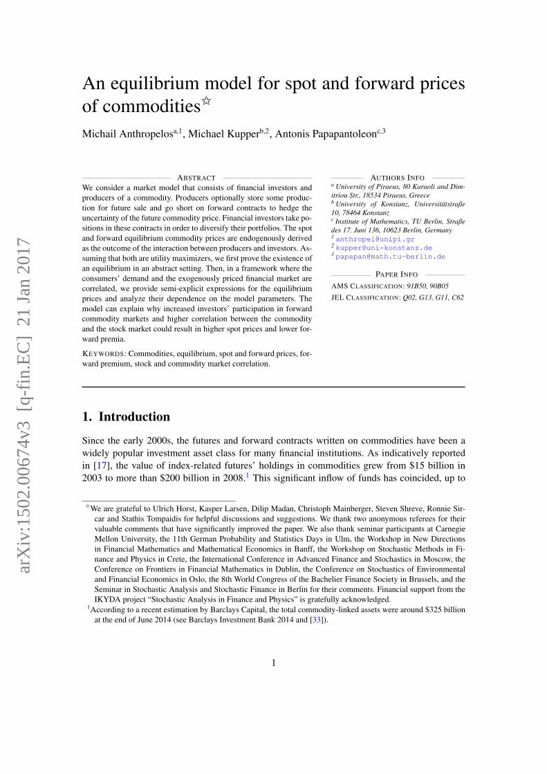
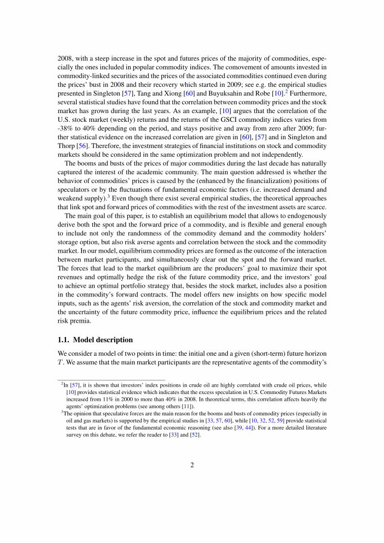
In this final section, we consider two specific models for the evolution of the financial market andthe consumers’ demand. The first one is driven by correlated Brownian motions and the secondone incorporates dependent jumps in addition. In the first case, we derive explicit expressionsfor the optimal storage policy and the optimal forward volume, and then the equilibrium pricefollows by the market clearing condition (2.12). In the second case, we derive semi-explicitexpressions for the optimal storage policy and the optimal forward volume, and the equilibriumprice is then computed numerically. Thereafter, we study the effect of the various parameters, inparticular the risk aversion coefficients of both agents and the production levels, in the formationof spot and forward prices.

24

5.1. A model driven by Brownian motion

In the first example, the dynamics of the variates X and Y determining the consumers demandand the financial market are driven by correlated Brownian motions. Specifically

Yt = b1t+ σ1W1t and Xt = σ2W

2t , (5.1)

where W 1,W 2 are standard Brownian motions with correlation ρ ∈ [−1, 1]. Moreover, using(2.8), the mean and variance of the spot price are given by

E[PT ] = φ0(πT )− α(1− ε)m

and Var[PT ] =σ2

2T

m2. (5.2)

The ensuing result provides an explicit expression for the optimal inventory policy and the opti-mal investment in the forward contract.

Proposition 5.1. Assuming the model dynamics provided by (5.1), the optimal strategy (α, hp)for the producers’ problem is given by

α =

(d3d5 − 2d2d4

4d1d4 − d23

∨ 0

)∧ π0 and hp = − αd3 + d5

2d4, (5.3)

while the optimal position hs for the investors’ problem equals

hs =E[PT ]− FγsVar[PT ]

− λρ√T

γs√Var[PT ]

. (5.4)

Here, the constants d1, . . . ,d5 are provided by (A.5) and γs = γs(1− ρ2).

The proof of the preceding Proposition is postponed for Appendix A.The equilibrium forward price F will be derived endogenously via the clearing condition

(2.12), where we should note that α, hp and hs all depend on F . Thereafter, the equilibrium spotprice of the commodity at the initial time is provided by

P0(F ) = φ0(π0) +α(F )

m. (5.5)

In this example, both the forward price and the optimal forward position are unique; this followsfrom Remark 3.7, Proposition 4.9 and the fact that up(α, ·) and us(α, ·) are strictly concave; seetheir explicit forms in (A.4) and (A.15).

Figures 5.1, 5.2 and 5.6 exhibit how the storage amount, the forward volume, the spot price,the forward premium and the convenience yield at the equilibrium depend on the correlationbetween the consumers’ demand and the financial market, as well as on the producers’ andinvestors’ risk aversion coefficients; see also the discussion in subsection 5.3.

Remark 5.2. Let us consider the case α∗ = 0. Then, the optimal position for the producerssimplifies to

hp(F ) =E[PT ]− FγpVar[PT ]

− πT (5.6)

25

and the clearing condition (2.12) yields that the equilibrium forward price is provided by

F = E[PT ]− γpγsγp + γs

Var[PT ]

(λρ√T

γs√Var[PT ]

+ πT

). (5.7)

Remark 5.3. In case there does not exist a forward contract that the producers could use forhedging—hence, there are also no investors in the market—the producers’ optimization problemtakes the form

Πpnf = max

α∈[0,π0]

d1α

2 + d2α+ d′3, (5.8)

where d1, d2 are given by (A.5). Therefore, the optimal storage strategy equals

α = (α∗ ∨ 0) ∧ π0 with α∗ = − d2

2d1, (5.9)

and the spot price of the commodity is

P0(α) = φ0(π0) +α

m.

5.2. A jump-diffusion model

In the next example, the dynamics of the variates that determine the consumers’ demand and thefinancial market are driven by a Lévy jump-diffusion process, where the Brownian motion rep-resents the ‘normal’ market behavior while the jumps appear simultaneously and represent some‘shocks’, e.g. news announcements, that affect both the financial asset price and the demand forthe commodity. More precisely, the dynamics of the processes Y and X are described by

Yt = b1t+ σ1W1t + η1Nt and Xt = b2t+ σ2W

2t + η2Nt, (5.10)

where the drift term equals bi = bi − ληi with bi, ηi ∈ R and σi ∈ R+, i = 1, 2. Furthermore,W 1,W 2 are standard Brownian motions with correlation ρ, while N is a univariate Poissonprocess with intensity λ ∈ R+. Hence, the constants η1 and η2 represent the effect of a jump inthe financial market and the demand for the commodity, respectively.

Moreover, assuming b2 = 0 as in the previous example, the expectation of XT equals zeroand using (2.8) we get that

E[PT ] = φ0(πT )− α(1− ε)m

and Var[PT ] =σ2

2 + λη22

m2T. (5.11)

Observe that the presence of jumps, either negative or positive, increases the variance of the spotprice PT relative to the Brownian motion example. The next result provides an expression forthe optimal inventory policy and the optimal investment in the forward contract.

26

−0.8 −0.6 −0.4 −0.2 0 0.2 0.4 0.6 0.86%

8%

10%

12%

14%

16%

18%

20%

22%

24%

correlation

optim

al s

tora

ge

γp=2

γp=4

γp=6

−0.8 −0.6 −0.4 −0.2 0 0.2 0.4 0.6 0.845%

50%

55%

60%

65%

70%

75%

80%

85%

90%

correlation

volu

me

in fo

rwar

d co

ntra

cts

γp=2

γp=4

γp=6

−0.8 −0.6 −0.4 −0.2 0 0.2 0.4 0.6 0.8correlation

equi

libriu

m s

pot p

rice

γp=2

γp=4

γp=6

−0.8 −0.6 −0.4 −0.2 0 0.2 0.4 0.6 0.80.2

0.3

0.4

0.5

0.6

0.7

0.8

0.9

1

correlation

forw

ard

prem

ium

γp=2

γp=4

γp=6

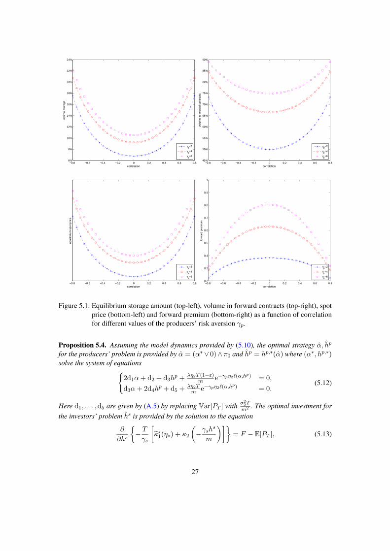
Figure 5.1: Equilibrium storage amount (top-left), volume in forward contracts (top-right), spotprice (bottom-left) and forward premium (bottom-right) as a function of correlationfor different values of the producers’ risk aversion γp.

Proposition 5.4. Assuming the model dynamics provided by (5.10), the optimal strategy α, hp

for the producers’ problem is provided by α = (α∗ ∨ 0)∧π0 and hp = hp,∗(α) where (α∗, hp,∗)solve the system of equations

2d1α+ d2 + d3hp + λη2T (1−ε)

m e−γpη2`(α,hp) = 0,

d3α+ 2d4hp + d5 + λη2T

m e−γpη2`(α,hp) = 0.

(5.12)

Here d1, . . . ,d5 are given by (A.5) by replacing Var[PT ] with σ22Tm2 . The optimal investment for

the investors’ problem hs is provided by the solution to the equation

∂

∂hs

− Tγs

[κs

1(η∗) + κ2

(−γsh

s

m

)]= F − E[PT ], (5.13)

27

−0.8 −0.6 −0.4 −0.2 0 0.2 0.4 0.6 0.80%

5%

10%

15%

20%

25%

correlation

optim

al s

tora

ge

γs=2

γs=4

γs=6

−0.8 −0.6 −0.4 −0.2 0 0.2 0.4 0.6 0.840%

45%

50%

55%

60%

65%

70%

75%

80%

85%

90%

correlation

volu

me

in fo

rwar

d co

ntra

cts

γs=2

γs=4

γs=6

−0.8 −0.6 −0.4 −0.2 0 0.2 0.4 0.6 0.8correlation

equi

libriu

m s

pot p

rice

γs=2

γs=4

γs=6

−0.8 −0.6 −0.4 −0.2 0 0.2 0.4 0.6 0.80.2

0.4

0.6

0.8

1

1.2

1.4

1.6

correlation

forw

ard

prem

ium

γs=2

γs=4

γs=6

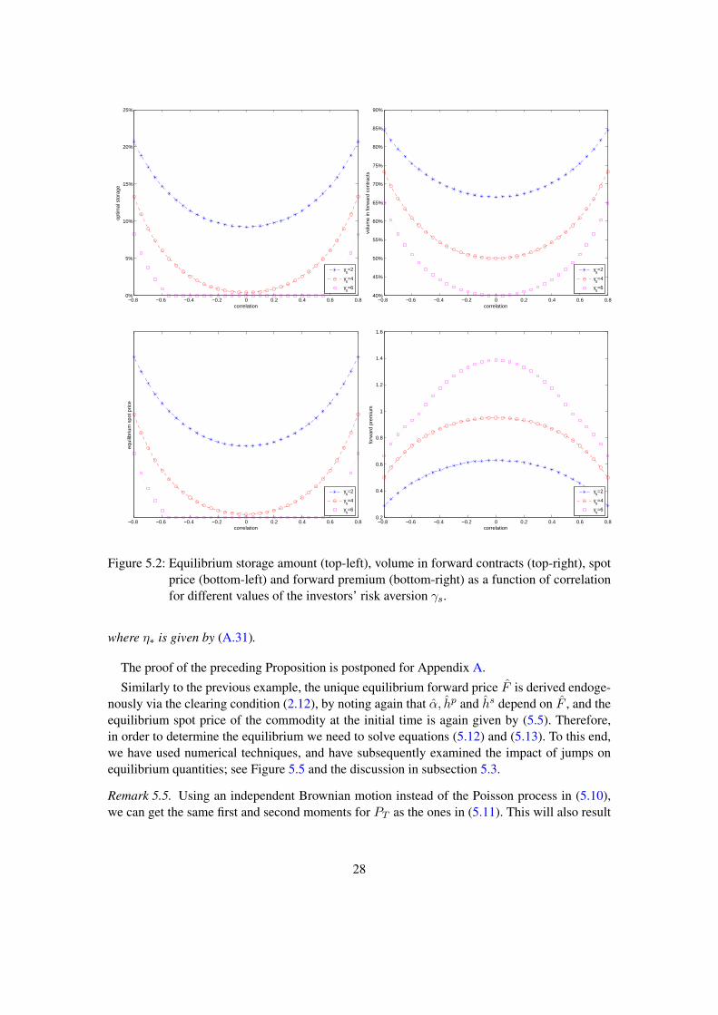
Figure 5.2: Equilibrium storage amount (top-left), volume in forward contracts (top-right), spotprice (bottom-left) and forward premium (bottom-right) as a function of correlationfor different values of the investors’ risk aversion γs.

where η∗ is given by (A.31).

The proof of the preceding Proposition is postponed for Appendix A.

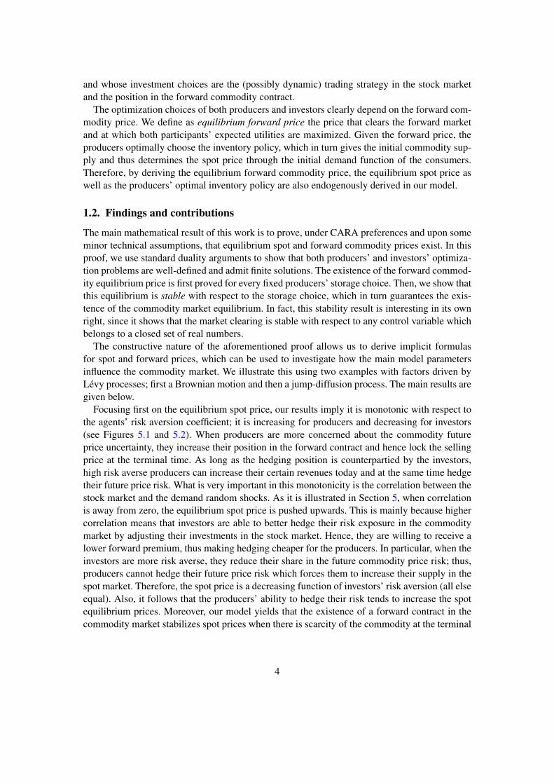
Similarly to the previous example, the unique equilibrium forward price F is derived endoge-nously via the clearing condition (2.12), by noting again that α, hp and hs depend on F , and theequilibrium spot price of the commodity at the initial time is again given by (5.5). Therefore,in order to determine the equilibrium we need to solve equations (5.12) and (5.13). To this end,we have used numerical techniques, and have subsequently examined the impact of jumps onequilibrium quantities; see Figure 5.5 and the discussion in subsection 5.3.

Remark 5.5. Using an independent Brownian motion instead of the Poisson process in (5.10),we can get the same first and second moments for PT as the ones in (5.11). This will also result

28

−0.8 −0.6 −0.4 −0.2 0 0.2 0.4 0.6 0.810%

15%

20%

25%

30%

35%

40%

45%

correlation

optim

al s

tora

ge w

hen

π T=

0.3π

0

With forwardWithout forward

−0.8 −0.6 −0.4 −0.2 0 0.2 0.4 0.6 0.810%

15%

20%

25%

30%

35%

40%

45%

correlation

optim

al s

tora

ge w

hen

π T=

0.6π

0

With forwardWithout forward

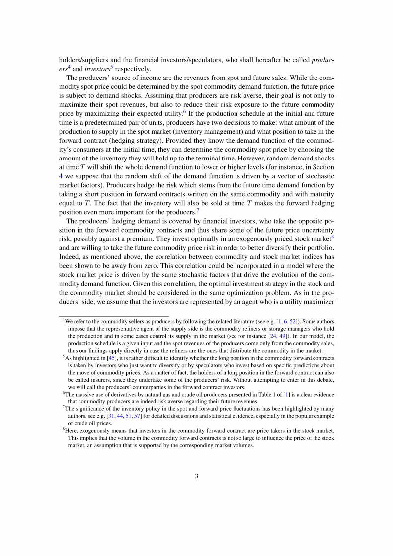
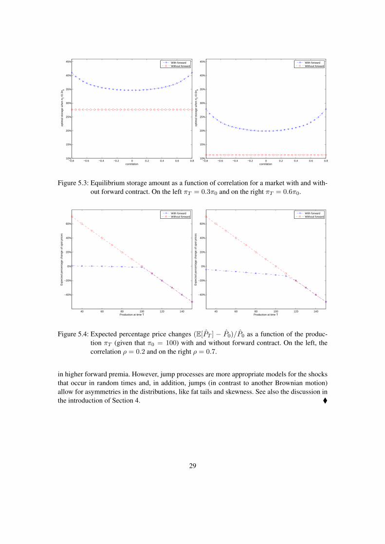
Figure 5.3: Equilibrium storage amount as a function of correlation for a market with and with-out forward contract. On the left πT = 0.3π0 and on the right πT = 0.6π0.

40 60 80 100 120 140

−40%

−20%

0%

20%

40%

60%

Production at time T

Exp

ecte

d pe

rcen

tage

cha

nge

of s

pot p

rices

With forwardWithout forward

40 60 80 100 120 140

−40%

−20%

0%

20%

40%

60%

Production at time T

Exp

ecte

d pe

rcen

tage

cha

nge

of s

pot p

rices

With forwardWithout forward

Figure 5.4: Expected percentage price changes (E[PT ] − P0)/P0 as a function of the produc-tion πT (given that π0 = 100) with and without forward contract. On the left, thecorrelation ρ = 0.2 and on the right ρ = 0.7.

in higher forward premia. However, jump processes are more appropriate models for the shocksthat occur in random times and, in addition, jumps (in contrast to another Brownian motion)allow for asymmetries in the distributions, like fat tails and skewness. See also the discussion inthe introduction of Section 4.

29

−0.8 −0.6 −0.4 −0.2 0 0.2 0.4 0.6 0.8correlation

spot

equ

ilibr

ium

pric

e

η2=−2

η2=0

η2=2

−0.8 −0.6 −0.4 −0.2 0 0.2 0.4 0.6 0.80.1

0.2

0.3

0.4

0.5

0.6

0.7

0.8

0.9

1

1.1

correlation

forw

ard

prem

ium

η2=−2

η2=0

η2=2

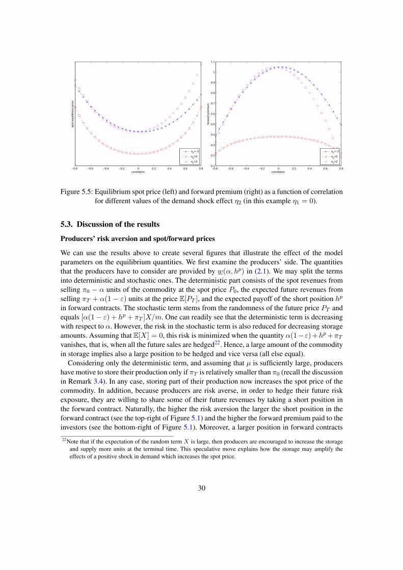
Figure 5.5: Equilibrium spot price (left) and forward premium (right) as a function of correlationfor different values of the demand shock effect η2 (in this example η1 = 0).

5.3. Discussion of the results

Producers’ risk aversion and spot/forward prices

We can use the results above to create several figures that illustrate the effect of the modelparameters on the equilibrium quantities. We first examine the producers’ side. The quantitiesthat the producers have to consider are provided by w(α, hp) in (2.1). We may split the termsinto deterministic and stochastic ones. The deterministic part consists of the spot revenues fromselling π0 − α units of the commodity at the spot price P0, the expected future revenues fromselling πT + α(1− ε) units at the price E[PT ], and the expected payoff of the short position hp

in forward contracts. The stochastic term stems from the randomness of the future price PT andequals [α(1− ε) + hp + πT ]X/m. One can readily see that the deterministic term is decreasingwith respect to α. However, the risk in the stochastic term is also reduced for decreasing storageamounts. Assuming that E[X] = 0, this risk is minimized when the quantity α(1−ε)+hp+πTvanishes, that is, when all the future sales are hedged22. Hence, a large amount of the commodityin storage implies also a large position to be hedged and vice versa (all else equal).

Considering only the deterministic term, and assuming that µ is sufficiently large, producershave motive to store their production only if πT is relatively smaller than π0 (recall the discussionin Remark 3.4). In any case, storing part of their production now increases the spot price of thecommodity. In addition, because producers are risk averse, in order to hedge their future riskexposure, they are willing to share some of their future revenues by taking a short position inthe forward contract. Naturally, the higher the risk aversion the larger the short position in theforward contract (see the top-right of Figure 5.1) and the higher the forward premium paid to theinvestors (see the bottom-right of Figure 5.1). Moreover, a larger position in forward contracts

22Note that if the expectation of the random term X is large, then producers are encouraged to increase the storageand supply more units at the terminal time. This speculative move explains how the storage may amplify theeffects of a positive shock in demand which increases the spot price.

30

implies an increasing tendency for storage, thus higher risk aversion leads to increased storageamounts (see the top-left of Figure5.1). Summarizing, even when the production levels at time 0and T are close, producers with higher risk aversion tend to store more of their production whenthey can hedge the risk of future sales, a result which is consistent with the theory of storage,and this strategy increases the spot price of the commodity (see the bottom-left of Figure 5.1).

This result is further supported by the model without a forward contract in the market, seeRemark 5.3. There, we observe that the only motive for the producers to store the commoditystems from the possible uneven productions (i.e. the difference between π0 and πT ). This motiveto store is increased when partial hedging is possible through the trading in forward contracts. Infact, as illustrated in Figure 5.3, the optimal storage is always higher in the model with forwardcontract, for every level of uneven productions, while for πT close to or higher than π0, theoptimal storage without forward contract is zero. Thus, spot prices in the model without forwardcontract are always lower compared to the model with forward. However, higher storage impliesthat the future expected spot price decreases (see for instance relation (5.2)), assuming that thereis no rolling of the position in the forward contracts. Hence, while forward contracts tend toincrease the spot commodity price, they also tend to decrease the future spot price. Therefore,the presence of forward contracts in the commodity market stabilizes prices when the productionlevels are uneven. This is apparent in Figure 5.4, where the expected price changes (E[PT ] −P0)/P0 are illustrated for different values of πT . In this example, we note that when there isscarcity of the commodity at time T , forward contracts serve to stabilize commodity spot prices.On the contrary, when the production at initial time is lower than that at terminal time, then theexpected price difference remains the same with and without the forward contract.

Let us also discuss the effect of jumps in the equilibrium quantities. Figure 5.5 illustrates theeffect of a possible side shock in the consumers’ demand stemming from a jump. This jump notonly increases the risk of the future price but it is also unhedgeable, since it is independent fromthe evolution of the stock market (we have assumed η1 = 0). Therefore, the forward premiumpaid to the investors is higher, irrespective of the sign of the jump (see the right part of Figure5.5). Moreover, when the future price is riskier, recalling the discussion above, we concludethat the more risk averse the producers are the more they increase the amount they store andhence they also increase the spot price of the commodity (see the left part of Figure 5.5). Inaddition, note that the sign of the jump makes little difference in the equilibrium quantities (ifthe expectation of the future demand shock is kept equal to zero).

The effect of the producers’ risk aversion on market equilibrium can be used to examine howthe number of producers affects the equilibrium commodity prices. In the present frameworkof CARA preferences, the parameter 1/γp measures the producers’ aggregate risk tolerance.Therefore, if the number of producers increases, the parameter γp decreases and the analysisabove implies that equilibrium spot prices are lower, as expected.

Investors’ risk aversion and spot/forward prices

Let us now examine the investors’ side. When they become more risk averse, they are lesswilling to undertake the risk of a forward position. This is illustrated in Figure 5.2 (top-right),where the percentage h/(πT + α) (i.e. the percentage of forward contracts with respect to thetotal supply at time T ) is plotted. Also, as the theory of normal backwardation states, more

31

risk averse investors would require higher forward premium to enter into the forward contract.This premium is usually measured by the fraction (E[PT ] − F )/F which is plotted in Figure5.2 (bottom-right). On the other hand, a higher forward premium implies that hedging is moreexpensive for the producers, hence they intend to supply more in the spot market and store less;note that the optimal storage amount even equals zero in some cases as the top-left of Figure 5.2shows). Summarizing, when investors are more risk averse they invest less in forward contracts,which reduces the amount that producers can use for hedging; thus, producers offer more on thespot market, rendering equilibrium spot prices lower (see the bottom-left of Figure 5.2).

Turning our attention to the effect of the correlation between the consumers’ demand and thefinancial markets’ return, we note that the equilibrium quantities mainly depend on the squareof ρ; this is basically because investors can go both long and short in the stock market. Whenρ2 increases, the effective risk aversion of the investors’, which is γs = γs(1 − ρ2), decreases.Therefore, an increase of ρ2 is eventually equivalent to a decrease of γs. This is expected becausewhen the financial and the commodity markets are correlated, the investors can partially hedgethe risk they undertake on a forward commodity contract by adjusting their investment strategyin the stock market accordingly. Hence, they become more risk tolerant. The dependence of theequilibrium quantities on the correlation coefficient ρ is illustrated in Figure 5.2.

The effect of the investors’ risk aversion on market equilibrium can be used to examine howthe number of investors affects the equilibrium commodity prices. In the present framework ofCARA preferences, the parameter 1/γs measures the investors’ aggregate risk tolerance. Hence,if the number of investors increases, the parameter γs considered in the above analysis decreases.As we have seen, the latter implies, among other things, higher equilibrium spot prices. Thistheoretical result is consistent with the observed comovement of the amounts invested in thecommodity forward contracts and the commodity spot prices (see the related discussion in theintroduction).

Convenience yield, correlation and uneven productions

As mentioned in the introduction, the convenience yield is a measure of the implicit benefit thatinventory holders receive. Positivity of the convenience yield is consistent with the theory ofstorage. In our model, the convenience yield denoted by y solves the equation

F = P01 +R

1− ε− yP0, (5.14)

see e.g. [1]. The relation of the yield with respect to the risk aversion coefficients of the producersand the investors is illustrated in Figure 5.6. As expected, y is increasing with respect to both riskaversion coefficients (all else equal). The relation for the producers’ side follows readily fromFigure 5.1, since higher producers’ risk aversion implies higher spot equilibrium price and higherforward premium (and also lower equilibrium forward price). Similarly, as the risk tolerance ofthe investors decreases, the cost of hedging increases, which makes producers sell more at thespot rather than storing and selling at a future date (see, in particular, the bottom-right of Figure5.2).

The relation of the yield with respect to the correlation coefficient is more involved. Whenρ2 increases, there are two effects of opposite directions on the convenience yield. The first is

32

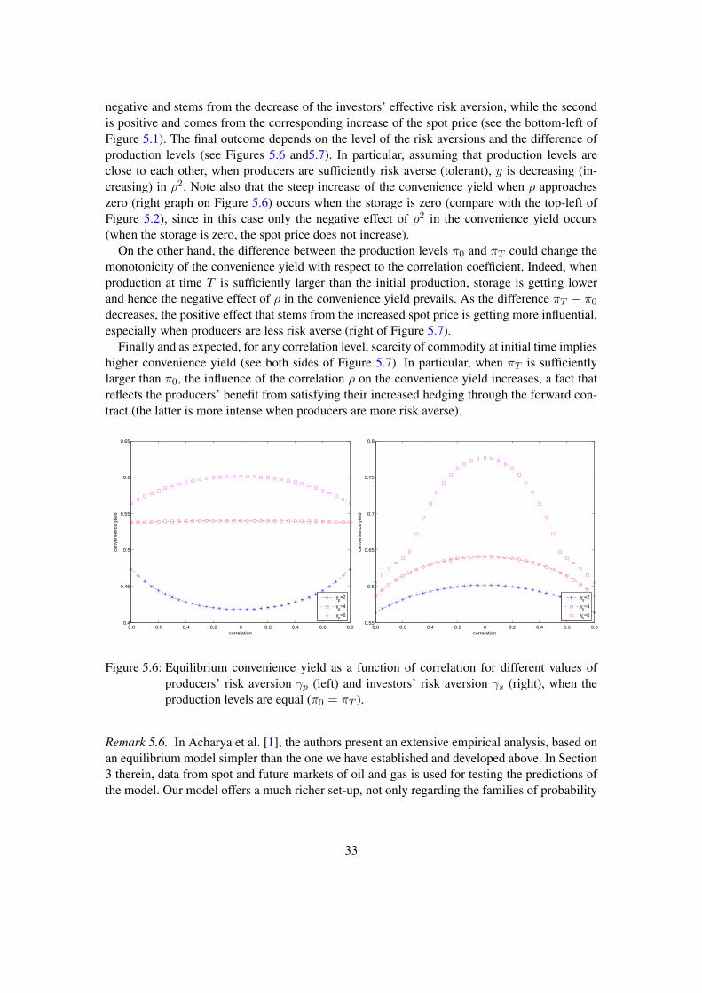
negative and stems from the decrease of the investors’ effective risk aversion, while the secondis positive and comes from the corresponding increase of the spot price (see the bottom-left ofFigure 5.1). The final outcome depends on the level of the risk aversions and the difference ofproduction levels (see Figures 5.6 and5.7). In particular, assuming that production levels areclose to each other, when producers are sufficiently risk averse (tolerant), y is decreasing (in-creasing) in ρ2. Note also that the steep increase of the convenience yield when ρ approacheszero (right graph on Figure 5.6) occurs when the storage is zero (compare with the top-left ofFigure 5.2), since in this case only the negative effect of ρ2 in the convenience yield occurs(when the storage is zero, the spot price does not increase).

On the other hand, the difference between the production levels π0 and πT could change themonotonicity of the convenience yield with respect to the correlation coefficient. Indeed, whenproduction at time T is sufficiently larger than the initial production, storage is getting lowerand hence the negative effect of ρ in the convenience yield prevails. As the difference πT − π0

decreases, the positive effect that stems from the increased spot price is getting more influential,especially when producers are less risk averse (right of Figure 5.7).

Finally and as expected, for any correlation level, scarcity of commodity at initial time implieshigher convenience yield (see both sides of Figure 5.7). In particular, when πT is sufficientlylarger than π0, the influence of the correlation ρ on the convenience yield increases, a fact thatreflects the producers’ benefit from satisfying their increased hedging through the forward con-tract (the latter is more intense when producers are more risk averse).

−0.8 −0.6 −0.4 −0.2 0 0.2 0.4 0.6 0.80.4

0.45

0.5

0.55

0.6

0.65

correlation

conv

enie

nce

yiel

d

γp=2

γp=4

γp=6

−0.8 −0.6 −0.4 −0.2 0 0.2 0.4 0.6 0.80.55

0.6

0.65

0.7

0.75

0.8

correlation

conv

enie

nce

yiel

d

γs=2

γs=4

γs=6

Figure 5.6: Equilibrium convenience yield as a function of correlation for different values ofproducers’ risk aversion γp (left) and investors’ risk aversion γs (right), when theproduction levels are equal (π0 = πT ).

Remark 5.6. In Acharya et al. [1], the authors present an extensive empirical analysis, based onan equilibrium model simpler than the one we have established and developed above. In Section3 therein, data from spot and future markets of oil and gas is used for testing the predictions ofthe model. Our model offers a much richer set-up, not only regarding the families of probability

33

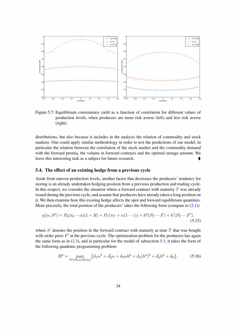
−0.8 −0.6 −0.4 −0.2 0 0.2 0.4 0.6 0.80.2

0.3

0.4

0.5

0.6

0.7

0.8

0.9

1

correlation

conv

enie

nce

yiel

d

π

T=0.6π

0

πT=π

0

πT=1.4π

0

−0.8 −0.6 −0.4 −0.2 0 0.2 0.4 0.6 0.80.2

0.3

0.4

0.5

0.6

0.7

0.8

0.9

1

correlation

conv

enie

nce

yiel

d

π

T=0.6π

0

πT=π

0

πT=1.4π

0

Figure 5.7: Equilibrium convenience yield as a function of correlation for different values ofproduction levels, when producers are more risk averse (left) and less risk averse(right).

distributions, but also because it includes in the analysis the relation of commodity and stockmarkets. One could apply similar methodology in order to test the predictions of our model, inparticular the relation between the correlation of the stock market and the commodity demandwith the forward premia, the volume in forward contracts and the optimal storage amount. Weleave this interesting task as a subject for future research.

5.4. The effect of an existing hedge from a previous cycle

Aside from uneven production levels, another factor that decreases the producers’ tendency forstoring is an already undertaken hedging position from a previous production and trading cycle.In this respect, we consider the situation where a forward contract with maturity T was alreadyissued during the previous cycle, and assume that producers have already taken a long position onit. We then examine how this existing hedge affects the spot and forward equilibrium quantities.More precisely, the total position of the producers’ takes the following form (compare to (2.1))

w(α, hp) = P0(π0 − α)(1 +R) + PT (πT + α(1− ε)) + hp(PT − F ) + h′(PT − F ′),(5.15)

where h′ denotes the position in the forward contract with maturity at time T that was boughtwith strike price F ′ at the previous cycle. The optimization problem for the producers has againthe same form as in (2.3), and in particular for the model of subsection 5.1, it takes the form ofthe following quadratic programming problem:

Πp = maxhp∈R,α∈[0,π0]

d1α

2 + d′2α+ d3αhp + d4(hp)2 + d′5h

p + d6

, (5.16)

34

where d1, d3,d4 remain the same and are provided by (A.5), while

d′2 =2(1 +R)π0 − (1− ε)(2πT + h′)− (R+ ε)µ

m− γp(1− ε)(πT + h′)Var[PT ]

d′5 = −(F − µ− πT

m

)− γp(πT + h′)Var[PT ].

We observe that an existing long position in the forward contract, i.e. h′ > 0, has the sameimpact as an increase of future production πT . Therefore, as in Figures 5.3, positive h′ impliesless storage and hence lower spot equilibrium price. In addition, as in Figure 5.7, when producershave already hedged some of their risk, the convenience yield increases, a fact that reflectsbetter inventory management. Similarly and as expected, a gradual hedging effectively serves tostabilize commodity prices (see Figure 5.4). This is because the tendency to increase spot pricesby forward contracts is gradually applied to prices. Intuitively, when producers hedge the futureprice uncertainty by rolling their position in the forward contract, the effect on the spot prices isspread through time. Note, however, that an intimate analysis on the gradually optimal hedgingrequires a dynamic version of our equilibrium model, which is left open for future research.

A. Proofs of Section 5

Proof (Proof of Proposition 5.1). The model with dynamics (5.1) fits in the framework of Sec-tion 4 by considering a 2-dimensional Brownian motion Z whose characteristic triplet has theform

b =

(b10

), c =

(σ2

1 ρσ1σ2

ρσ1σ2 σ22

)and ν ≡ 0, (A.1)

where b ∈ R, σ1, σ2 ∈ R+ and ρ ∈ [−1, 1], while the vectors u1, u2 ∈ R2 have the form

u1 =

(10

)and u2 =

(01

). (A.2)

The cumulant generating functions of Y1 = 〈u1, Z1〉 and X1 = 〈u2, Z1〉 are given by

κ1(v) = vb1 +v2σ2

1

2and κ2(v) =

v2σ22

2. (A.3)

The set UZ equals R2, thus Assumption (EM) and (3.23) are trivially satisfied, while the sameis true for Assumption (FE) since ν ≡ 0. Assumption (COE) is also satisfied due to κ2 beingquadratic in u, while Assumption (NA′) is fulfilled since we can construct a martingale measureunder which Z remains a Brownian motion.

Starting with the producers’ side, the optimal hedging and storage positions are determinedby Proposition 3.2 and (4.8), leading to the following quadratic programming problem:

Πp = maxhp∈R,α∈[0,π0]

d1α

2 + d2α+ d3αhp + d4(hp)2 + d5h

p + d6

, (A.4)

35

where

d1 = −(

1 +R+ (1− ε)2

m+γp(1− ε)2

2Var[PT ]

)d2 =

2(1 +R)π0 − 2(1− ε)πT − (R+ ε)µ

m− γp(1− ε)πT Var[PT ]

d3 = −1− εm− γp(1− ε)Var[PT ] (A.5)

d4 = −γp2

Var[PT ]

d5 = −(F − µ− πT

m

)− γpπT Var[PT ].

The first order conditions yield the following solutions

hp,∗ = −αd3 + d5

2d4and α∗ =

d3d5 − 2d2d4

4d1d4 − d23

. (A.6)

Therefore, the optimal strategy (α, hp) ∈ [0, π0]×R for the producers’ problem is provided by

α = (α∗ ∨ 0) ∧ π0 and hp = − αd3 + d5

2d4. (A.7)

Next, we turn our attention to the investors’ problem and follow the strategy outlined in sub-section 4.2. The cumulant generating function of Z under Ps is provided by

κs(v) = 〈v − ξ, b〉+〈v − ξ, c(v − ξ)〉

2, (A.8)

where ξ = −γshs

m u2. In particular, the characteristics of Y under Ps are

bs1 = b1 − ρσ1σ2

γshs

mand cs

1 = σ21, (A.9)

thus the characteristics of the exponential transform Y under Ps are

bs1 = b1 − ρσ1σ2

γshs

m+σ2

1

2and cs

1 = σ21. (A.10)

The cumulant generating function of Y simply has the form

κs1(v) = v

(b1 − ρσ1σ2

γshs

m+σ2

1

2

)+v2σ2

1

2, (A.11)

and its derivative obviously equals

∂

∂vκs

1(v) = b1 − ρσ1σ2γsh

s

m+σ2

1

2+ vσ2

1. (A.12)

36

Therefore, the solution to equation (4.18) is

η∗ = ρσ2

σ1

γshs

m− b1σ2

1

− 1

2, (A.13)

and the minimal entropy equals

H(P∗|Ps) =T

2(η∗σ1)2 =

T

2

(λ− ρσ2

γshs

m

)2. (A.14)

Here λ denotes the ‘market price of risk’ for the asset S, i.e. λ = µ1−rσ1

, with µ1 being theexpected rate of return of S and r the continuously compounded interest rate, while we havealso used that b1 = µ1 − r − σ2

1/2.The investors’ optimal position in the forward contract is determined by (4.24), leading to the

following quadratic optimization problem:

Πs = maxhs∈R

d7(hs)2 + d8h

s + d9

, (A.15)

where

d7 = −γs2

(1− ρ2)Var[PT ] (A.16)

d8 = E[PT ]− F − λρ√T√

Var[PT ]. (A.17)

Applying the first order conditions once again, we arrive at the optimal position for the investors

hs =E[PT ]− FγsVar[PT ]

− λρ√T

γs√Var[PT ]

, (A.18)

where γs = γs(1− ρ2).

Proof (Proof of Proposition 5.4). The model with dynamics (5.10) fits in the framework of Sec-tion 4 by considering a 2-dimensional Lévy process Z whose characteristic triplet has the form

b =

(b1b2

), c =

(σ2

1 ρσ1σ2

ρσ1σ2 σ22

)and ν(dx1, dx2) = λ1η1,η2(dx1, dx2), (A.19)

while the vectors u1, u2 ∈ R2 are provided by (A.2). The cumulant generating function ofY1 = 〈u1, Z1〉 and X1 = 〈u2, Z1〉 is given by

κi(v) = vbi +v2σ2

i

2+ λ (evηi − 1) i = 1, 2. (A.20)

The set UZ equals R2, thus Assumption (EM) and (3.23) are trivially satisfied, while the sameis true for Assumption (FE). Assumption (COE) is also satisfied due to κ2 being quadratic in v,

37

while Assumption (NA′) is satisfied since we can construct a martingale measure under whichX has finite first moment.

Starting with the producers side, the optimal hedging and storage positions are provided byProposition 3.2 and (4.8), leading to the following optimization problem:

Πp = maxhp∈R,α∈[0,π0]

f(α, hp) (A.21)

where

f(α, hp) := d1α2 + d2α+ d3αh

p + d4(hp)2 + d5hp + d6 + j(α, hp), (A.22)

with

j(α, hp) := −λ(

e−γpη2`(α,hp) − 1

) Tγp. (A.23)

The coefficients d1, . . . ,d5 are provided by (A.5) by replacing Var[PT ] with σ22Tm . The first order

optimality conditions lead to the system of non-linear equations (5.12), i.e.∂∂αf(α, hp) = 2d1α+ d2 + d3h

p + λη2T (1−ε)m e−γpη2`(α,h

p) = 0,∂∂hp f(α, hp) = d3α+ 2d4h

p + d5 + λη2Tm e−γpη2`(α,h

p) = 0,(A.24)

and its solution is denoted by (α∗, hp,∗), where the relation of α∗ and hp,∗ is given by the fol-lowing linear equation

α∗ =2(1− ε)d4 − d3

2d1 − (1− ε)d3hp,∗ +

(1− ε)d5 − d2

2d1 − (1− ε)d3.

Therefore, the optimal strategy (α, hp) ∈ [0, π0]× R for the producers problem is provided by

α = (α∗ ∨ 0) ∧ π0 and hp = hp,∗(α). (A.25)

Next, we turn our attention to the investors problem and follow again the strategy of subsection4.2. The characteristics of Y under Ps are provided by Lemma 4.2, thus using (A.19) we get that

bs1 = b1 − ρσ1σ2ζ + λη1(e−η2ζ − 1)

cs1 = σ2

1 (A.26)

1E(y) ∗ νs1 = 1E(〈u1, x〉)e〈ξ,x〉 ∗ ν,

where ζ := γshs

m , E ∈ B(R) and “∗” denotes integration. Therefore, the cumulant generatingfunction of Y under Ps takes the form

κs1(v) = vbs

1 +v2σ2

1

2+ λ(evη1 − 1)e−ζη2 . (A.27)

38

Moreover, the characteristics of the exponential transform Y of Y are provided by (4.14), thuswe obtain that

bs1 = κs

1(1)

cs1 = σ2

1 (A.28)

1E(z) ∗ νs1 = 1E(ey − 1) ∗ νs

1.

Hence, the cumulant generating function of Y under Ps equals

κs1(v) = vbs

1 +v2σ2

1

2+ λe−η2ζ

(ev(eη1−1) − 1

)(A.29)

and its derivative with respect to v equals

∂

∂vκs

1(v) = bs1 + vσ2

1 + λe−η2ζev(eη1−1)(eη1 − 1). (A.30)

The minimal entropy martingale measure is determined by the solution η∗ to the non-linearequation

bs1 + η∗σ

21 + λe−η2ζeη∗(e

η1−1)(eη1 − 1) = 0, (A.31)

and then the minimal entropy equals

H(P∗|Ps) = − Tγsκs

1(η∗). (A.32)

Now, putting the pieces together, the investors optimization problem takes the form

Πs = maxhs

g(hs) (A.33)

where

g(hs) := − Tγs

κs

1(η∗) + κ2

(−γsh

s

m

)+ hs

(E[PT ]− F

), (A.34)

and the maximizer is determined by the first order conditions, leading to (5.13).

References[1] V.V. Acharya, A.L. Lochstoer, and T. Ramadorai. Limits to arbitrage and hedging: Evidence from

commodity markets. Journal of Financial Economics, 109:441–465, 2013.[2] R.W. Anderson and J.-P. Danthine. Hedging and joint production: Theory and illustrations. Journal

of Finance, 35:487–498, 1980.[3] R.W. Anderson and J.-P. Danthine. Hedger diversity in futures markets. Economic Journal, 93:

370–389, 1983.[4] M. Anthropelos and G. Žitkovic. On agent’s agreement and partial-equilibrium pricing in incom-

plete markets. Mathematical Finance, 20:411–446, 2010.

39

[5] D. Applebaum. Lévy Processes and Stochastic Calculus. Cambridge University Press, 2nd edition,2009.

[6] S. D. Baker. The financialization of storable commodities. Preprint, ssrn:2348333, 2014.[7] P. Barrieu and N. El Karoui. Pricing, hedging and designing derivatives with risk measures. In

R. Carmona, editor, Indifference Pricing: Theory and Applications, pages 77–145. Princeton Uni-versity Press, 2009.

[8] S. Basak and A. Pavlova. A model of financialization of commodities. Journal of Finance, 2016.(forthcoming).

[9] M. Brennan. The supply of storage. American Economic Review, 48:50–72, 1958.[10] B. Buyuksahin and M.A. Robe. Speculators, commodities and cross-market linkages. Journal of

International Money and Finance, 42:38–70, 2014.[11] R. Caldentey and M. Haugh. Optimal control and hedging of operations in the presence of financial

markets. Mathematics of Operations Research, 31:285–304, 2006.[12] P. Carr, H. Geman, D. B. Madan, and M. Yor. The fine structure of asset returns: An empirical

investigation. Journal of Business, 75:305–332, 2002.[13] J. Casassus, P. Collin-Dufresne, and B. Routledge. Equilibrium commodity prices with irreversible

investment and non-linear technologies. NBER Working Paper No. 11864, 2008.[14] P. Cheridito. Convex analysis. Lecture notes, Princeton University, 2013.[15] P. Cheridito, U. Horst, M. Kupper, and T. Pirvu. Equilibrium pricing in incomplete markets under

translation invariant preferences. Mathematics of Operations Research, 41:174–195, 2016.[16] A. S. Cherny and A. N. Shiryaev. Change of time and measure for Lévy processes. Lecture Notes,

University of Aarhus, 2002.[17] Staff Report on Commodity Swap Dealers and Index Traders with Commission Recommendations.

Commodity Futures Trading Commission, 2008.[18] R. Cont and P. Tankov. Financial Modelling with Jump Processes. Chapman and Hall/CRC Press,

2004.[19] F. Delbaen, P. Grandits, T. Rheinländer, D. Samperi, M. Schweizer, and C. Stricker. Exponential

hedging and entropic penalties. Mathematical Finance, 12:99–123, 2002.[20] E. Eberlein. Application of generalized hyperbolic Lévy motions to finance. In O. E. Barndorff-

Nielsen, T. Mikosch, and S. I. Resnick, editors, Lévy Processes: Theory and Applications, pages319–336. Birkhäuser, 2001.

[21] E. Eberlein and K. Glau. Variational solutions of the pricing PIDEs for European options in Lévymodels. Applied Mathematical Finance, 21:417–450, 2014.

[22] E. Eberlein and J. Jacod. On the range of options prices. Finance and Stochastics, 1:131–140,1997.

[23] E. Eberlein, A. Papapantoleon, and A. N. Shiryaev. Esscher transform and the duality principle formultidimensional semimartingales. Annals of Applied Probability, 19:1944–1971, 2009.

[24] I. Ekeland, D. Lautier, and B. Villeneuve. Speculation in commodity futures markets: A simpleequilibrium model. Working paper, Université Paris-Dauphine, 2014.

[25] D. Filipovic and M. Kupper. Equilibrium prices for monetary utility functions. International Jour-nal of Theoretical and Applied Finance, 11:325–343, 2008.

[26] H. Föllmer and A. Schied. Stochastic Finance. de Gruyter, 2nd edition, 2004.[27] T. Fujiwara. From the minimal entropy martingale measures to the optimal strategies for the expo-

nential utility maximization: the case of geometric Lévy processes. Asia-Pacific Financial Markets,11:367–391, 2004.

40

[28] T. Fujiwara and Y. Miyahara. The minimal entropy martingale measures for geometric Lévy pro-cesses. Finance and Stochastics, 7:509–531, 2003.

[29] G. B. Gorton and K. G. Rouwenhorst. Facts and Fantasies about Commodity Futures. FinancialAnalysts Journal, 62:47–68, 2006.

[30] G. B. Gorton, F. Hayashi, and K. G. Rouwenhorst. The fundamentals of commodity futures returns.Review of Finance, 17:35–105, 2012.

[31] J. D. Hamilton. Causes and consequences of the oil shock of 2007–08. Brookings Papers onEconomic Activity, 1:215–261, 2009.

[32] J. D. Hamilton and C. Wu. Effects of index-fund investing on commodity futures prices. Interna-tional Economic Review, 56:187–205, 2015.

[33] B.J. Henderson, N.D. Pearson, and L. Wang. New evidence on the financialization of commoditymarkets. Review of Financial Studies, 28:1285–1311, 2015.

[34] J.R. Hicks. Value and Capital. Oxford University Press, 1939.[35] D. Hirshleifer. Residual risk, trading costs, and commodity futures risk premiums. Review of

Financial Studies, 1:173–193, 1988.[36] D. Hirshleifer. Futures trading, storage and the division of risk: A multiperiod analysis. Economic

Journal, 99:700–719, 1989.[37] U. Horst and M. Müller. On the spanning property of risk bonds priced by equilibrium. Mathematics

of Operations Research, 32:784–807, 2007.[38] F. Hubalek and C. Sgarra. Esscher transforms and the minimal entropy martingale measure for

exponential Lévy models. Quantitative Finance, 6:125–145, 2006.[39] L. Juvenal and I. Petrella. Speculation in oil market. Working paper, Federal Reserve Bank of Saint

Louis, 2012.[40] N. Kaldor. Speculation and economic stability. Review of Economic Studies, 7:1–27, 1939.[41] J. Kallsen and A. N. Shiryaev. The cumulant process and Esscher’s change of measure. Finance

and Stochastics, 6:397–428, 2002.[42] I. Karatzas, J.P. Lehoczky, and S.E. Shreve. Existence and uniqueness of multi-agent equilibrium

in a stochastic, dynamic consumption/investment model. Mathematics of Operations Research, 15:80–128, 1990.

[43] J.M. Keynes. A Treatise on Money, Vol. 2. Macmillan, London, 1930.[44] L. Kilian and D.P. Murphy. The role of inventories and speculative trading in the global market for

crude oil. Journal of Applied Econometrics, 29:454–478, 2014.[45] C. Knittel and R. Pindyck. The simple economics of commodity price speculation. NBER Working

Paper No. 18951, 2013.[46] A. E. Kyprianou. Introductory Lectures on Fluctuations of Lévy Processes with Applications.

Springer, 2006.[47] R.J.A. Laeven and M. Stadje. Robust portfolio choice and indifference valuation. Mathematics of

Operations Research, 39:1109–1141, 2014.[48] E. Leclercq and R. Praz. Equilibirum commodity trading. Preprint, ssrn:2464400, 2014.[49] C. Pirrong. Commodity Price Dynamics: A Structural Approach. Cambridge University Press,

2011.[50] R. T. Rockafellar. Convex Analysis. Princeton University Press, 1997.[51] B.R. Routledge, D.J. Seppi, and C.S. Spatt. Equilibrium forward curves for commodities. Journal

of Finance, 60:1297–1338, 2000.[52] K.G. Rouwenhorst and K. Tang. Commodity Investing. Annual Review of Financial Economics, 4:

447–467, 2012.

41

[53] K. Sato. Lévy Processes and Infinitely Divisible Distributions. Cambridge University Press, 1999.[54] W. Schoutens. Lévy Processes in Finance: Pricing Financial Derivatives. Wiley, 2003.[55] A. N. Shiryaev. Essentials of Stochastic Finance: Facts, Models, Theory. World Scientific, 1999.[56] A. Singleton and S. Thorp. Financialization, crisis and commodity correlation dynamics. Journal

of International Financial Markets, Institutions and Money, 24:42–65, 2013.[57] K. J. Singleton. Investor flows and the 2008 boom/bust in oil prices. Management Science, 60:

300–318, 2014.[58] H. Stoll. Commodity futures and spot price determination and hedging in capital market equilib-

rium. Journal of Financial and Quantitative Analysis, 14:873–894, 1979.[59] H. Stoll and R. Whaley. Commodity index investing and commodity futures prices. Journal of

Applied Finance, 20:7–46, 2010.[60] K. Tang and W. Xiong. Index investing and the financialization of commodities. Financial Analysts

Journal, 68(6):54–74, 2012.[61] R. Wilson. The theory of syndicates. Econometrica, 36:119–132, 1968.[62] H. Working. The theory of the price of storage. American Economic Review, 39:1254–1262, 1949.

42