Transaction Costs and Asset Prices:

A Dynamic Equilibrium Model

Dimitri Vayanos∗

August 1997

∗MIT Sloan School of Management, 50 Memorial Drive E52-437, Cambridge MA 02142-1347,

tel 617-2532956, e-mail dimitriv@mit.edu. I thank Anat Admati, Peter Bossaerts, George Con-

stantinides (the referee), Peter DeMarzo, Darrell Duffie, Sanford Grossman, John Heaton, Ravi

Jagannathan (the editor), David Kreps, Costis Skiadas, Matthew Spiegel, and Jiang Wang, seminar

participants at Berkeley, Chicago, MIT, Northwestern, Pittsburgh, Stanford, Toulouse, and Whar-

ton, and participants at the European Econometric Society, WFA, and NBER General Equilibrium

and Asset Pricing Conferences, for very helpful comments and suggestions. I also thank Francesco

Giovannoni, Lee-Bath Nelson, and Muhamet Yildiz for excellent research assistance.

Abstract

In this paper we study the effects of transaction costs on asset prices. We

assume an overlapping generations economy with a riskless, liquid bond, and

many risky stocks carrying proportional transaction costs. We obtain stock

prices and turnover in closed-form. Surprisingly, a stock’s price may increase in

transaction costs, and a more frequently traded stock may be less adversely af-

fected by an increase in transaction costs. Calculations based on the “marginal”

investor overestimate the effects of transaction costs. For realistic parameter

values, transaction costs have very small effects on stock prices but large effects

on turnover.

1

Transaction costs such as bid-ask spreads, brokerage commissions, market impact

costs, and transaction taxes, are important in many financial markets.1 Moreover,

considerable attention has focused on their effects on asset prices. A recent example

is the debate on how prices of NYSE stocks would be affected if a transaction tax is

imposed.2 Transaction costs have also been proposed as an explanation for various

asset pricing puzzles such as the equity premium puzzle (Mehra and Prescott (1985))3

and the small stock puzzle (Banz (1981) and Reinganum (1981)).4

Although transaction costs are mentioned in many asset pricing debates, they are

generally absent from asset pricing models. Some papers introduce transaction costs,

but assume that assets are identical in all other dimensions.5 This assumption is

restrictive. In the equity premium puzzle for instance, stocks are riskier than bonds,

while in the small stock puzzle, small stocks are not perfectly correlated with large

stocks. Some other papers relax the assumption that assets differ only in transaction

costs, assuming instead a riskless, perfectly liquid bond, and a risky stock that carries

transaction costs.6 These papers treat asset prices as exogenous and determine the

optimal investment policy. They also compare the rate of return on the stock to

the rate of return that a perfectly liquid stock should have, so that the investor is

indifferent between the two stocks. However, the difference between the two rates can

be interpreted as the effect of transaction costs, only when the investor is constrained

to choose one of the two stocks and cannot diversify. In addition, the analysis is

not done in a general equilibrium setup where both stocks are present and prices are

endogenous. Heaton and Lucas (1996) endogenize asset prices in an one bond/one

stock model, but have to resort to numerical methods.

In this paper we develop a general equilibrium model with transaction costs. We

assume a riskless, perfectly liquid bond with a constant rate of return, and many

risky stocks that carry proportional transaction costs. Trade occurs because there

are overlapping generations of investors who buy the assets when born and slowly

sell them until they die. The model is very tractable and stock prices are obtained in

closed-form.

Our results are surprising and contrary to “conventional wisdom” about the effects

of transaction costs on asset prices. First, the price of a stock may increase in its

2

transaction costs. An increase in transaction costs has two opposing effects on the

stock’s demand. On the one hand, investors buy fewer shares, but on the other, they

hold them for longer periods. We show that either effect can dominate.

According to conventional wisdom, the effect of transaction costs on the stock

price depends on the stock’s minimum holding period, i.e. the holding period of the

marginal investor. For the marginal investor to be induced to buy the stock, the

price has to fall by the present value of transaction costs that he, and all future

marginal investors, incur (the “PV term”).7 Our second result is, however, that the

PV term overstates the effect of transaction costs on the stock price. The reason is

that, with transaction costs, investors hold the stock for longer periods. Therefore

the marginal investor holds fewer shares and requires a smaller risk premium. The

difference between the effect of transaction costs and the PV term is important and

should not be neglected in practical applications. For small transaction costs ε, the

effect of transaction costs is of order ε, while the PV term is of order√

ε.

Our third result is about how the effect of transaction costs on the stock price,

depends on the stock’s characteristics. According to conventional wisdom, a more

liquid stock or a riskier stock is more adversely affected by an increase in its trans-

action costs. Indeed, since such a stock is traded more frequently, the holding period

of the marginal investor is shorter and the PV term larger. We show, however, that

a more frequently traded stock may be less adversely affected by an increase in its

transaction costs. The reason is that the marginal investor greatly reduces his stock

holdings and requires a smaller risk premium. An empirical implication of our results

is that a cross-sectional regression of asset returns on transaction costs should include

the following two terms with opposite signs: (i) a nonlinear term in transaction costs8

and (ii) an interaction term between transaction costs and asset risk.

Our fourth result concerns the effect of a change in one stock’s transaction costs

on the price of another stock. According to conventional wisdom, if transaction costs

of a stock decrease, the price of a less liquid but correlated stock should increase,

since agents do not need to trade it as much. We show, however, that the price

may decrease. This result suggests that the introduction of a low transaction cost

derivative (such as an option or a futures contract) may decrease the price of the

3

underlying asset.9

In addition to stock prices, we study stock turnover and obtain it in closed-form.

A stock’s turnover decreases in the stock’s transaction costs and increases in the

transaction costs of other stocks. One would expect turnover to increase in the

stock’s risk, since investors would face a higher cost of deviating from their optimal,

no transaction cost, portfolio. We show, however, that turnover may decrease.

Finally, we calibrate the model. For realistic parameter values, transaction costs

have very small effects on stock prices but large effects on investors’ trading strategies

and turnover. In addition, turnover is small, because it is generated only by lifecycle

effects. Our results are very similar to Constantinides (1986) and Barclay, Kandel,

and Marx (1997).

The rest of the paper is structured as follows: in section 1, we present the model. In

section 2 we study agents’ optimization problem and market-clearing, and determine

a simple set of conditions that are sufficient for equilibrium. In section 3 we construct

the equilibrium in the benchmark case where there are no transaction costs. In section

4 we construct the equilibrium in the case where there are transaction costs. We then

study the effects of transaction costs on stock prices and turnover. In section 5 we

extend the analysis to the case where the short-sale constraint for some stocks is

binding. In section 6 we calibrate the model. Section 7 concludes, and most proofs

are in the Appendix.

4

1 The Model

We consider a continuous time overlapping generations economy. Time, t, goes from

−∞ to ∞. There is a continuum of agents. Each agent lives for an interval of

length T . Between times t and t + dt, dt/T agents are born and dt/T die. The total

population is thus 1.

1.1 Financial Assets

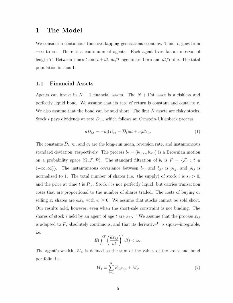
Agents can invest in N + 1 financial assets. The N + 1’st asset is a riskless and

perfectly liquid bond. We assume that its rate of return is constant and equal to r.

We also assume that the bond can be sold short. The first N assets are risky stocks.

Stock i pays dividends at rate Di,t, which follows an Ornstein-Uhlenbeck process

dDi,t = −κi(Di,t −Di)dt + σidbi,t. (1)

The constants Di, κi, and σi are the long-run mean, reversion rate, and instantaneous

standard deviation, respectively. The process bt = (b1,t, ., bN,t) is a Brownian motion

on a probability space (Ω,F ,P). The standard filtration of bt is F = Ft : t ∈(−∞,∞). The instantaneous covariance between bi,t and bj,t is ρi,j , and ρi,i is

normalized to 1. The total number of shares (i.e. the supply) of stock i is si > 0,

and the price at time t is Pi,t. Stock i is not perfectly liquid, but carries transaction

costs that are proportional to the number of shares traded. The costs of buying or

selling xi shares are εixi, with εi ≥ 0. We assume that stocks cannot be sold short.

Our results hold, however, even when the short-sale constraint is not binding. The

shares of stock i held by an agent of age t are xi,t.10 We assume that the process xi,t

is adapted to F , absolutely continuous, and that its derivative11 is square-integrable,

i.e.

E(∫ T

0

(

dxi,t

dt

)2

dt) < ∞.

The agent’s wealth, Wt, is defined as the sum of the values of the stock and bond

portfolio, i.e.

Wt ≡N∑

i=1

Pi,txi,t + Mt. (2)

5

1.2 Endowments and Preferences

Agents are born with an endowment y of a consumption good, and do not receive any

other endowment over their lifetime. They derive utility from lifetime consumption.

Consumption takes the form of a flow ct for t ∈ [0, T ] and a “gulp” CT for t = T . We

assume that the process ct is adapted to F , continuous, and square-integrable, i.e.

E(∫ T

0c2t dt) < ∞.

Utility over consumption is exponential, i.e.

u(ct, CT ) = −∫ T

0e−act−βtdt− e−ACT−βT . (3)

We assume a “smooth” utility e−ACT−βT , rather than the constraint CT ≥ 0 that

is more standard and corresponds to A = ∞, for technical reasons. We assume,

however, that A is large in order to obtain qualitatively similar results to the case

A = ∞.

The assumptions that are essential to the tractability of the model are the follow-

ing. First, the riskless rate is constant. Second, dividends follow Ornstein-Uhlenbeck

processes and are thus normal. Third, utility over consumption is exponential, and

fourth transaction costs are proportional to the number of shares, rather than the

dollar value. These assumptions turn out to imply two key properties of the equilib-

rium, namely that stock prices are linear in dividends and that agents’ stock holdings

are deterministic.

The assumptions of constant riskless rate, normal dividends, and exponential util-

ity are admittedly special. However they are almost standard in market microstruc-

ture theory.12 They are also used in dynamic asset pricing theory13 since they are

one of the very few sets of assumptions under which the CAPM holds. This paper

shows that, under such standard assumptions, the effects of transaction costs can be

contrary to conventional wisdom.

6

2 Optimization and Market-Clearing

In this section we study agents’ optimization problem and market-clearing, and de-

termine a simple set of conditions that are sufficient for equilibrium.

2.1 Optimization

We first state the optimization problem. We then determine a set of conditions that

are sufficient for optimality.

2.1.1 The Optimization Problem

To simplify the optimization problem, we immediately assume the equilibrium dy-

namics of the stock prices, Pi,t. In equilibrium Pi,t is given by

Pi,t = P i +Di,t −Di

r + κi

. (4)

The stock price, Pi,t, is a long-run mean, P i, plus a linear function of the deviation

of the dividend, Di,t, from its own long-run mean, Di. The sensitivity of Pi,t w.r.t.

Di,t is 1/(r + κi), and is decreasing in the riskless rate, r, and the reversion rate, κi.

This is intuitive: if r and κi are high, an increase in the current dividend has a small

effect on the present value of future dividends. The instantaneous standard deviation

of Pi,t is σi/(r + κi). By appropriately redefining a share of each stock we can change

σi, and adopt the normalizationσi

r + κi

= 1. (5)

An agent chooses stock holdings, xi,t, and consumption, ct, to maximize expected

utility. The dynamics of his wealth, Wt, are given by

dWt =N∑

i=1

(Di,tdt + dPi,t)xi,t + rMtdt− ctdt−N∑

i=1

εi

∣

∣

∣

∣

∣

dxi,t

dt

∣

∣

∣

∣

∣

dt. (6)

Using equations 1, 2, 4, and 5, we can simplify the wealth dynamics to

dWt =N∑

i=1

(Di − rP i)xi,tdt +N∑

i=1

xi,tdbi,t + rWtdt− ctdt−N∑

i=1

εi

∣

∣

∣

∣

∣

dxi,t

dt

∣

∣

∣

∣

∣

dt. (7)

The first term in the RHS corresponds to the excess return on the stock portfolio

relative to the bond. The second term corresponds to the portfolio’s risk. The third

7

term corresponds to the return if all wealth were invested in the bond. The fourth

and fifth terms correspond to the consumption and transaction costs respectively.

Notice that, due to the dividend and price dynamics 1 and 4 respectively, the divi-

dends, Di,t, do not enter in the wealth dynamics 7. Therefore, stock holdings, xi,t,

will be independent of the Di,t’s. Since utility is exponential, the xi,t’s will also be

independent of wealth, Wt. The xi,t’s will only be functions of the agent’s age, and

thus deterministic. This is a key simplifying property of the equilibrium.

At time 0 the agent buys xi,0 shares of stock i. His bond holdings thus are

M0 = y −N∑

i=1

(Pi,0 + εi)xi,0. (8)

Equations 2 and 8 imply that the agent’s initial wealth is

W0 = y −N∑

i=1

εixi,0, (9)

i.e. initial wealth, W0, is equal to the endowment, y, minus the transaction costs. At

time T the agent sells xi,T shares of stock i. Equation 2 implies that the consumption

gulp is

CT = MT +N∑

i=1

(Pi,T − εi)xi,T = WT −N∑

i=1

εixi,T . (10)

Therefore the agent’s optimization problem, (P), is

sup(xi,t,ct)

−E(∫ T

0e−act−βtdt + e−ACT−βT )

subject to

dWt =N∑

i=1

(

(Di − rP i)xi,tdt + xi,tdbi,t

)

+ rWtdt− ctdt−N∑

i=1

εi

∣

∣

∣

∣

∣

dxi,t

dt

∣

∣

∣

∣

∣

dt,

W0 = y −N∑

i=1

εixi,0,

CT = WT −N∑

i=1

εixi,T ,

and the short-sale constraint xi,t ≥ 0.

8

2.1.2 The Optimality Conditions

We now study the optimization problem (P). The main tool for studying consump-

tion/investment problems with transaction costs is dynamic programming. Dynamic

programming is used, for instance, in all the papers that assume one stock, and are

cited in footnote 6. With many stocks, however, dynamic programming becomes very

complex. The state space becomes large, since one state variable must be introduced

for each stock. We will study (P) using the calculus of variations instead of dynamic

programming. More precisely, we will determine a set of sufficient conditions for a

control (xi,t, ct) to be locally optimal. Since (P) is concave, the control (xi,t, ct) will

be globally optimal. We determine the sufficient conditions in proposition 1, proven

in appendix A. Before stating the proposition we define γ = 1− ra/A, and At by

At =ra

1− γe−r(T−t). (11)

At corresponds to the coefficient of absolute risk-aversion of an agent of age t. Since

A is large, γ ∈ (0, 1) and At increases with age t. Agents are more risk-averse when

old because with a shorter horizon their consumption reacts more to an adverse price

shock.

Proposition 1 Consider N continuous and piecewise C1 functions xi,t in [0, T ]. Sup-

pose that for each xi,t there exist 0 ≤ ti < ti ≤ T such that

(i) xi,t = xi,0 > 0 ∀t ∈ [0, ti], dxi,t/dt < 0 ∀t ∈ [ti, ti], and xi,t = 0 ∀t ∈ (ti, T ],

(ii)∫ ti

0(Di − rP i + rεi − At

N∑

j=1

ρi,jxj,t)e−rtdt− 2εi = 0, (12)

(iii)

Di − rP i + rεi − At

N∑

j=1

ρi,jxj,t = 0 ∀t ∈ [ti, ti], (13)

(iv) At

∑Nj=1 ρi,jxj,t increases ∀t ∈ [0, ti],

and

(v)

Di − rP i + rεi − At

N∑

j=1

ρi,jxj,t ≤ 0 ∀t ∈ (ti, T ]. (14)

Then there exists ct, such that (xi,t, ct) solves (P).

9

Proposition 1 provides a set of sufficient conditions for stock holdings, xi,t, to be

part of an optimal control. Condition (i) states that holdings of stock i are constant

in an interval [0, ti], strictly decreasing in [ti, ti], and 0 in (ti, T ]. The agent thus buys

stock i when born, and sells it slowly between ti and ti. He sells the stock as he gets

older because he becomes more risk-averse. He starts selling at ti rather than 0, i.e.

not immediately after he buys, because of transaction costs. If ti < T , the agent

does not hold stock i in an interval (ti, T ] of positive length. In fact, the short-sale

constraint for stock i is binding in this interval. In the next sections we show that

the short-sale constraint is binding, if stock i is highly correlated with other stocks

that have larger transaction costs.

Conditions (ii) to (v) are first-order conditions. Condition (ii) is a first-order

condition for the shares of stock i, xi,0, that the agent buys when born. This condition

states that the agent’s payoff does not change in the first order if he buys some

additional shares at time 0 and sells them at time ti. Indeed, we can write condition

(ii) as∫ ti

0(Di − rP i − At

N∑

j=1

ρi,jxj,t)e−rtdt− εi(1 + e−rti) = 0. (15)

The first term inside the integral, Di− rP i, corresponds to the increase in the excess

return on the stock portfolio, from buying the additional shares. The second term

corresponds to the increase in risk. It is the product of stock i’s contribution to

portfolio risk,∑N

j=1 ρi,jxj,t, times the coefficient of absolute risk-aversion, At. The

last term corresponds to the transaction costs incurred at times 0 and ti. All terms

are discounted at interest rate r.

Condition (iii) is a first-order condition for the shares of stock i, xi,t, that the

agent holds at time t ∈ [ti, ti], i.e. when he is selling the stock. This condition states

that the agent’s payoff does not change in the first order if he sells some shares at

time t + dt rather than at time t. Indeed, multiplying by dt, we can write condition

(iii) as

(Di − rP i)dt− At

N∑

j=1

ρi,jxj,tdt + rεidt = 0.

The first term corresponds to the increase in excess return from holding the shares

until time t + dt. The second term corresponds to the increase in risk. The last term

10

corresponds to the savings from incurring the transaction cost at time t + dt rather

than at time t. Condition (iv) ensures that the agent’s payoff decreases if he buys

some additional shares at time 0 and sells them at time t < ti, or if he sells some

shares at time t < ti rather than at time ti. Finally, condition (v) ensures that the

agent’s payoff decreases if he sells some shares during the “short-sale interval” (ti, T ]

rather than at time ti.

2.2 Market-Clearing

We first study market-clearing in a “stock” sense and then in a “flow” sense. The

market for stock i clears in a “stock” sense if total holdings at a given point in time

are equal to the stock’s supply. To compute total holdings, we note that there are

dt/T agents with age between t and t + dt, and each holds xi,t shares. Therefore, the

market clears in a “stock” sense if

∫ T

0xi,t

dt

T= si. (16)

The market for stock i clears in a “flow” sense if the number of shares bought in a

given time interval is equal to the number of shares sold. If condition 16 is satisfied,

the market clears in a “stock” sense at each point in time, and thus automatically

clears in a “flow” sense. A more direct and perhaps more intuitive way to show that

the market clears in a “flow” sense, is to compute the number of shares of stock i

bought and sold between times t and t + dt. For the number of shares bought, we

note that the buyers are the agents born between t and t + dt. Since there are dt/T

such agents and each buys xi,0 shares, the number of shares bought is xi,0dt/T . For

the number of shares sold, we note that the sellers are the agents who at time t have

age greater than ti. Since at time t + dt these agents have age greater than ti + dt,

they collectively own xi,tidt/T fewer shares. Therefore the number of shares sold is

xi,tidt/T and is equal to the number of shares bought. The turnover of stock i, Vi, is

defined as the stock’s trading volume between times t and t + dt, divided by dt and

by the stock’s supply. It is equal to

Vi =xi,0

Tsi

. (17)

11

To construct the equilibrium in the next sections, we determine numbers P i and

functions xi,t that satisfy the following simple set of sufficient conditions. First,

conditions (i) to (v) of proposition 1, and second, the market-clearing conditions 16.

12

3 Equilibrium Without Transaction Costs

In this section we study the benchmark case where the εi’s are zero. We construct the

equilibrium in proposition 2. Before stating the proposition, we define the function

f(t) by

f(t) =ra

T

(

t

At

+∫ T

t

ds

As

)

. (18)

The function f(t) corresponds to total stock holdings when agents start selling at

time t.

Proposition 2 Define P i by

P i =Di

r− a

∑Nj=1 ρi,jsj

f(0)(19)

and xi,t by

xi,t = si

ra

f(0)At

. (20)

Then the conditions of proposition 1 and the market-clearing conditions hold.

Proof: Equation 11 implies that the xi,t’s are C1 in [0, T ]. Condition (i) of

proposition 1 holds since the xi,t’s are strictly decreasing in [0, T ] and thus ti = 0 and

ti = T . The only other condition of proposition 1 left to check is (iii). Equations

19 and 20 imply that it holds. Finally, equations 18 and 20 imply that the market-

clearing conditions 16 hold. Q.E.D.

The equilibrium has a very simple form. Consider first equation 20 that gives

agents’ stock holdings. To obtain stock holdings at age s, we simply need to multiply

stock holdings at age t by At/As. Therefore all agents hold the same stock portfolio,

which is the market portfolio. Agents buy the market portfolio when born and sell it

slowly until they die. Turnover is the same for all stocks.14 Indeed, the definition of

turnover, i.e. equation 17, and equation 20, imply that the turnover of stock i is

Vi =xi,0

Tsi

=ra

Tf(0)A0

.

The pricing equation 19 has the CAPM flavor. Stock i’s price, P i, is the present

value of the dividend, Di, minus a risk premium. The risk premium depends on

the coefficient of absolute risk-aversion, a, and the stock’s systematic risk, i.e. its

covariance with the market portfolio,∑N

j=1 ρi,jsj.

13

4 Equilibrium With Transaction Costs

In this section we study the case where the εi’s are not zero, and the short-sale

constraint is not binding. In the next section we extend the analysis to the case

where the short-sale constraint is binding.

To construct the equilibrium, we make 3 assumptions. The first 2 assumptions

ensure that the short-sale constraint is not binding. The constraint will be binding

if stocks are highly correlated but differ substantially in transaction costs. Indeed,

because of the high correlation, the gains to diversification are small. The optimal

investment is determined by transaction cost considerations, with low transaction

cost stocks being sold first and the other stocks afterwards. Assumption 1 ensures

that there are gains to diversification, i.e. stocks are not perfectly correlated.

Assumption 1 The correlation matrix

1 . ρ1,N

. .

ρN,1 . 1

(21)

is positive definite.

Assumption 2 ensures that the gains to diversification are larger than the differences

in transaction costs. For notational simplicity, we state the assumption in terms of

the stock prices, P i, that are endogenous and defined in proposition 3.

Assumption 2 For P i’s defined by equation 28, the column vector

1 . ρ1,N

. .

ρN,1 . 1

−1

D1 − rP 1 + rε1

.

DN − rPN + rεN

(22)

is strictly positive.

To motivate the vector 22, assume that stocks are highly positively correlated but dif-

fer substantially in transaction costs. Assume, for instance, that stock 1 has the low-

est transaction costs. Since stocks are highly positively correlated, the non-diagonal

terms of the correlation matrix are negative and large. Since, in addition, stock 1

14

has lower transaction costs than the other stocks, the first term of the vector 22 is

negative, and assumption 2 is violated. Assumption 2 is satisfied in the no transaction

costs case. Indeed, equation 19 implies that

f(0)

ra

D1 − rP 1

.

DN − rPN

=

1 . ρ1,N

. .

ρN,1 . 1

s1

.

sN

.

Therefore, the vector 22 is simply (ra/f(0))(s1, ., sN ) > 0. By continuity, assumption

2 is always satisfied for small transaction costs.

Our third assumption is

Assumption 3 For any b1, ., bi ⊆ 1, ., N, the non-diagonal terms of the

matrix

1 . ρb1,bi

. .

ρbi,b1 . 1

−1

(23)

are negative.

Assumption 3 implies that the stocks are substitutes in the following strong sense.

Suppose that there are no transaction costs and that agents can only invest in stocks

b1, ., bi and in the bond. The demand for a stock has then to increase in the price of

another stock. Indeed, equation 13 implies that the demand of an agent of age t is

given by

1

At

1 . ρb1,bi

. .

ρbi,b1 . 1

−1

Db1 − rP b1

.

Db1 − rP bi

.

An implication of assumption 3, obtained by setting i = 2, is that ρj,k ≥ 0, i.e. stocks

are positively correlated. Assumption 3 is satisfied, for instance, when ρj,k = ρ ≥0, ∀j, k, j 6= k. Besides being quite realistic, assumption 3 ensures that stock holdings

are (weakly) decreasing with age, a key simplifying property of the equilibrium.15 In

section 4.1 we construct the equilibrium, and in sections 4.2 and 4.3 we study the

effects of transaction costs on stock prices and turnover.

15

4.1 Construction of the Equilibrium

We first give some useful definitions. We define the function g(t) by

g(t) =∫ t

0(1− As

At

)e−rsds. (24)

The function g(t) corresponds to the benefit of buying an additional share at time 0

and selling it at t, gross of transaction costs. We also define the function I(ζ, b, b1, ., bi)for ζ = (ζ1, ., ζN ), b1, ., bi ⊆ 1, ., N, and b ∈ 1, ., N, by

I(ζ, b, b1, ., bi) = ζb − (ρb,b1 , ., ρb,bi)

1 . ρb1,bi

. .

ρb1,bi. 1

−1

ζb1

.

ζbi

. (25)

The vector ζ in this definition will be the transaction costs vector ε = (ε1, ., εN ), or a

linear combination of the correlation vectors ρ.,j = (ρ1,j , ., ρN,j).

We now construct the ti’s, i.e. the times at which the agents start selling the stocks

or, equivalently, the stocks’ minimum holding periods. Without loss of generality, we

assume that stock 1 minimizesεk

∑Nj=1 ρk,jsj

over all stocks k. Therefore it has small transaction costs, ε1, and large systematic

risk,∑N

j=1 ρ1,jsj. Stock 1 is the first stock that agents start selling, and t1 is defined

byg(t1)

f(t1)=

2

ra

ε1∑N

j=1 ρ1,jsj

.

Agents start selling stock 1 first because this is the cheapest way to reduce portfolio

risk. Similarly, we assume that stock 2 minimizes

εk − ρk,1ε1∑N

j=1 ρk,jsj − ρk,1∑N

j=1 ρ1,jsj

over all stocks k ≥ 2. Therefore, in addition to having small transaction costs and

large systematic risk, it has a small correlation with stock 1. Stock 2 is the second

stock that agents start selling, and t2 is defined by

g(t2)

f(t2)=

2

ra

ε2 − ρ2,1ε1∑N

j=1 ρ2,jsj − ρ2,1∑N

j=1 ρ1,jsj

.

16

To generalize this construction, we set Si = 1, ., i and S0 = ∅, and assume that

stock i minimizesI(ε, k, Si−1)

I(∑N

j=1 ρ.,jsj, k, Si−1)(26)

over all stocks k ≥ i. Stock i is the i’th stock that agents start selling, and ti is

defined byg(ti)

f(ti)=

2

ra

I(ε, i, Si−1)

I(∑N

j=1 ρ.,jsj, i, Si−1). (27)

In proposition 3 we construct the stock prices, P i, and stock holdings, xi,t. Proposition

3 is proven in appendix B.

Proposition 3 If A is large, then 0 ≤ t1 ≤ . ≤ tN < T . Define P i by

P i =Di

r+ εi − a

i∑

k=1

I(∑N

j=1 ρ.,jsj, k, Sk−1)

f(tk)

I(ρ.,i, k, Sk−1)

I(ρ.,k, k, Sk−1)(28)

and xi,t recursively by

x1,t

.

xN,t

=1

At

1 . ρ1,N

. .

ρN,1 . 1

−1

D1 − rP 1 + rε1

.

DN − rPN + rεN

(29)

for t ∈ [tN , T ] and

xk,t = xk,tk k ≥ i,

x1,t

.

xi−1,t

=1

At

1 . ρ1,i−1

. .

ρi−1,1 . 1

−1

D1 − rP 1 + rε1

.

Di−1 − rP i−1 + rεi−1

−

1 . ρ1,i−1

. .

ρi−1,1 . 1

−1

ρ1,i . ρ1,N

. .

ρi−1,i . ρi−1,N

xi,t

.

xN,t

(30)

for t ∈ [ti−1, ti] (t0 = 0). Then all conditions of proposition 1 and the market-clearing

conditions hold.

Equations 29 and 30 give agents’ stock holdings for t ∈ [tN , T ] and t ∈ [0, tN ],

respectively. For t ∈ [0, t1] holdings of all stocks are constant. For t ∈ [t1, t2] holdings

17

of stocks 2 to N are constant, while holdings of stock 1 decrease. Agents use only

stock 1 to reduce portfolio risk. More generally, for t ∈ [ti−1, ti] holdings of stocks i

to N are constant, while holdings of stocks 1 to i− 1 decrease. Finally, for t ∈ [tN , T ]

holdings of all stocks decrease. With transaction costs, the composition of the stock

portfolio depends on age. Low transaction cost stocks, held for short periods, are

mainly in the portfolios of young agents, while high transaction cost stocks, held for

long periods, are in the portfolios of old agents. Equation 28 gives stock prices in

closed-form. In sections 4.2 and 4.3 we use equations 28, 29, and 30 to study the

effects of transaction costs on stock prices and turnover.

4.2 Stock Prices

In this section we study how a stock’s price depends on its and other stocks’ trans-

action costs. Propositions 4 and 5 examine how the stock’s price depends on its

transaction costs, and how the effect of transaction costs depends on the stock’s char-

acteristics. Both propositions are proven in appendix C. Before stating the proposi-

tions we define T1 by (2 + γ)− 3γe−rT1 − rT1 = 0, and T2 by 2γe−rT2 − 1 = 0.16

Proposition 4 If T ≤ T1, then P i decreases in εi. If T > T1, then P i increases for

small εi, and decreases for large εi.

The surprising result of proposition 4 is that a stock’s price does not always

decrease in its transaction costs. If T is large and εi small, it increases. To provide an

intuition for proposition 4 we assume that there is only one stock and that transaction

costs increase from ε1 to ε′1 > ε1. In figure 1 we plot agents’ stock holdings as a

function of age, for ε1 and the corresponding equilibrium price P 1 (solid line), and for

ε′1 and P 1 (dashed line). When transaction costs increase, agents buy fewer shares,

i.e. x′1,0 < x1,0. However, they hold these shares for longer periods, i.e. they hold

x shares for t′1,x > t1,x. Total stock holdings, i.e. the area under each curve, may

thus increase or decrease. Stock holdings increase when T is large because agents

are selling during a very long period. Therefore, the effect that they sell more slowly

dominates the effect that they buy fewer shares.

INSERT FIGURE 1 SOMEWHERE HERE

18

Proposition 5 If T ≤ T2, then ∂P i/∂εi increases in ti. If T > T2, then ∂P i/∂εi

decreases for small εi, and may increase for large εi.

Proposition 5 shows that a stock with a shorter minimum holding period, ti, is not

always more adversely affected by an increase in its transaction costs. If T is large

and εi small, it is less adversely affected. In corollary B.2, proven in appendix B, we

show that a stock’s ti increases in its transaction costs, εi, and decreases in its supply,

si, which is a measure of the stock’s risk. Proposition 5 thus implies that more liquid

stocks or riskier stocks may be less adversely affected by increases in their transaction

costs. This result is surprising since these stocks are more frequently traded.

To provide an intuition for proposition 5, we examine the first-order condition for

the shares of stock i, xi,0, that an agent buys when born (i.e. equation 15). We can

write this equation as

P i =Di

r− εi

1 + e−rti

1− e−rti−∫ ti0 At

∑Nj=1 ρi,jxj,te

−rtdt

1− e−rti, (31)

and interpret it as a pricing equation. Stock i’s price, P i, has to be such that the

agent is induced to buy the marginal xi,0’th share and hold it for t ≤ ti. Equation 31

is a valuable tool for providing intuition for our results.

Equation 31 shows that the price, P i, is the present value of the dividend, Di,

minus two terms. The first term compensates the agent for transaction costs. We

call this term the “PV term”, and write it as

εi(1 + 2e−rti + 2e−2rti + .).

This is equal to the present value of the following transaction costs. First, the costs

that the agent incurs buying and selling the xi,0’th share, at times 0 and ti. Second,

the costs that the next agent who buys the share incurs, at times ti and 2ti, and so

on. According to conventional wisdom, the effect of transaction costs on the stock

price is equal to the PV term.

The second term compensates the agent for buying a risky stock, and is thus a

risk premium. The risk premium increases in the stock’s contribution to portfolio

risk,∑N

j=1 ρi,jxj,t, for t ≤ ti, and in the coefficient of absolute risk-aversion, At. Very

importantly, the risk premium changes with transaction costs. Indeed, the lifetime

19

pattern of stock holdings changes. As figure 1 shows, agents buy fewer shares and

hold them for longer periods. Therefore they hold fewer shares for t ≤ ti, and the

risk premium decreases. The PV term thus overstates the effect of transaction costs

on the stock price. The difference between the effect of transaction costs and the PV

term is important and should not be neglected in practical applications. Equation

28 shows that the effect of transaction costs is of order ε, while the PV term is of

order√

ε.17 The PV term measures correctly the effect of transaction costs in two

special cases. First, when agents are risk-neutral (Amihud and Mendelson (1986))

and second, when stocks are riskless (Vayanos and Vila (1997)). In both cases the

risk premium is zero.

Equation 31 shows why a stock with a shorter minimum holding period, ti, may

be less adversely affected by an increase in its transaction costs. On the one hand,

the PV term increases more in response to an increase in transaction costs. On the

other hand, agents greatly reduce their stock holdings during the shorter minimum

holding period. Therefore the risk premium decreases more, and the overall effect is

ambiguous.

Corollary 1 and proposition 6 examine how a stock’s price, P i, depends on the

transaction costs of the other stocks, εk. Corollary 1 examines the case i < k and is

proven in appendix B, while proposition 6 examines the case i > k and is proven in

appendix C.

Corollary 1 P i is independent of εk for i < k.

Corollary 1 shows that a stock’s price is independent of the transaction costs

of less liquid stocks. If εk increases, agents buy fewer shares of stock k and hold

them for longer periods. To adjust for that change, they buy more shares of stock i

and hold them for shorter periods. Since stock i is more liquid, agents can exactly

“undo” the change in their holdings of stock k and keep stock i’s contribution to

portfolio risk,∑N

j=1 ρi,jxj,t, unchanged for each time t. (This is easiest to see in

the extreme case where εi = 0. In that case ti = 0, and equation 13 implies that∑N

j=1 ρi,jxj,t = (Di − rP i)/At, ∀t, independently of εk.) Therefore ti, the PV term,

the risk premium, and P i remain unchanged.

20

Proposition 6 If T ≤ T2, then P i decreases in εk, for i > k. If T > T2, then P i

increases for small εi, εk, and may decrease for large εi, εk.

Proposition 6 shows that a stock’s price does not always decrease in the transaction

costs of more liquid stocks. If T is large and εi, εk small, it increases. To provide a

simple intuition for this result, we note that that if εk increases, stock i will be

traded more frequently. Therefore, by proposition 5, it may be more or less adversely

affected by its own transaction costs, i.e. its price may decrease or increase. We

can also provide a more direct intuition using equation 31. If εk increases, agents

buy fewer shares of stock k and hold them for longer periods. Since stock i is less

liquid, agents cannot “undo” the change in their holdings of stock k, and start selling

stock i earlier. Therefore ti decreases (as we show in corollary B.2) and the PV term

increases. At the same time, since agents buy fewer shares of stock k and stock i is

positively correlated with stock k, the risk premium decreases, and the overall effect

is ambiguous.

A natural conjecture is that changes in transaction costs of the most liquid stocks

have the strongest effect on the prices of the other stocks, since they affect most

agents’ portfolios. Corollary 2 shows that this conjecture is true in the special case

ρi,j = ρ ≥ 0, ∀i, j, i 6= j. The corollary follows from proposition 6 and is proven in

appendix C.

Corollary 2 Suppose that ρi,j = ρ ≥ 0, ∀i, j, i 6= j. If T ≤ T2, then ∂P i/∂εk

increases in k for k < i. If T > T2, then ∂P i/∂εk decreases for small εi, εk, but may

increase for large εi, εk.

Corollary 2 shows that if the correlation between all stocks is the same, the effect

on P i of an increase in εk is stronger (either more negative or more positive) the

more liquid k is. The corollary cannot be extended to the case where the correlations

between stocks differ. We can choose, for instance, the most liquid stock to be

independent of the other stocks, so that an increase in its transaction costs does not

affect their price.

21

4.3 Stock Turnover

In this section we study stock turnover, defined by equation 17. We compute turnover

in proposition 7, proven in appendix D.

Proposition 7 The turnover of stock i is

Vi =xi,0

Tsi

=ra

Tsi

(

1

f(ti)Ati

I(∑N

j′=1 ρ.,j′sj′ , i, Si−1)

I(ρ.,i, i, Si−1)

−N∑

j=i+1

1

f(tj)Atj

I(∑N

j′=1 ρ.,j′sj′ , j, Sj−1)

I(ρ.,j , j, Sj−1)

I(ρ.,j, i, Sj−1\i)I(ρ.,i, i, Sj−1\i)

. (32)

Proposition 8 examines how a stock’s turnover depends on its and other stocks’

transaction costs. The proposition is proven in appendix D.

Proposition 8 Vi decreases in εi and increases in εk for k 6= i

The intuition for proposition 8 is simple. If εi increases, Vi decreases since agents

buy fewer shares of stock i and hold them for longer periods. If εk increases, agents

buy fewer shares of stock k and hold them for longer periods. To adjust for that

change, they buy more shares of stock i and sell them faster, i.e. Vi increases. The

result that Vi increases in εk depends crucially on assumption 3, i.e. that stocks are

substitutes.

We also examine how Vi depends on stock i’s risk, as measured, for instance, by

the stock’s supply, si. If si increases, ti decreases, i.e. agents start selling the stock

earlier. One would thus expect Vi to increase. Vi may however decrease, if stock

i is correlated with other stocks that have higher transaction costs. To economize

on trading these stocks, agents hold a large fraction of stock i initially and a small

fraction later. If si increases, gains to diversification become more important than

economizing on transaction costs, and agents have to hold stock i for longer periods.

Therefore Vi may decrease. Using equation 32, one can check that Vi increases with

si when, for instance, stock i is independent of the other stocks, while Vi decreases

when there are two stocks, i = 1, ρ1,2 > 0, and ε1 = 0.

22

5 Binding Short-Sale Constraint

In this section we extend the analysis to the case where the short-sale constraint

is binding. For simplicity we assume that there are only two positively correlated

stocks, and set ρ1,2 = ρ ∈ [0, 1]. Assumption 1’ ensures that the short-sale constraint

is binding.

Assumption 1′ Suppose that ρ < 1 and

εi

si + ρsj

≤ εj

sj + ρsi

for i 6= j ∈ 1, 2. Then, for P i and P j defined by equation 28,

Di − rP i + rεi − ρ(Dj − rP j + rεj) ≤ 0. (33)

Assumption 1′ is the “opposite” of assumptions 1 and 2 of section 4, i.e. the parame-

ters s1, s2, ε1, ε2, and ρ ∈ [0, 1] satisfy assumption 1′ if and only if they do not satisfy

assumptions 1 or 2.18 In section 5.1 we construct the equilibrium, and in section 5.2

we study the effects of transaction costs on stock prices.

5.1 Construction of the Equilibrium

Without loss of generality, we assume that

ε1

s1 + ρs2

≤ ε2

s2 + ρs1

. (34)

i.e. stock 1 has a smaller ratio of transaction costs to systematic risk than stock 2.

Stock 1 is the first stock that the agents start selling. Condition 34 is the same as in

section 4. However, now it implies that ε1 ≤ ε2, i.e. stock 1 has smaller transaction

costs than stock 2.19 In proposition 9 we construct the stock prices and stock holdings.

Proposition 9 is proven in appendix E.

Proposition 9 If A is large, the equations

g(t1)(D1 − rP 1 + rε1)− 2ε1 = 0, (35)

g(t2)(D2 − rP 2 + rε2)− 2ε2 − ρ(g(t1)(D1 − rP 1 + rε1)− 2ε1) = 0, (36)

23

D1 − rP 1 + rε1

At1

− ρD2 − rP 2 + rε2

At2

= 0, (37)

f(t1)− f(t1)

ra(D1 − rP 1 + rε1) = s1, (38)

andf(t2)

ra(D2 − rP 2 + rε2) = s2, (39)

have a solution, (t1, t1, t2, P 1, P 2), such that 0 ≤ t1 < t1 ≤ t2 < T . Define x2,t by

x2,t =D2 − rP 2 + rε2

At

∀t ∈ [t2, T ] and x2,t = x2,t2 ∀t ∈ [0, t2). (40)

Define also x1,t by

x1,t = 0 ∀t ∈ [t1, T ],

x1,t =D1 − rP 1 + rε1

At

− ρx2,t ∀t ∈ [t1, t1), and x1,t = x1,t1 ∀t ∈ [0, t1). (41)

Then all conditions of proposition 1 and the market-clearing conditions hold.

Equations 40 and 41 give agents’ holdings of stocks 2 and 1 respectively. Agents

start selling stock 1 first at time t1. By time t1 they own no shares of stock 1 and the

short-sale constraint becomes binding. Agents start selling stock 2 at time t2. The

stock prices, P 1 and P 2, are jointly determined with the times t1, t1, and t2, by the

non-linear system of equations 35 to 39.

5.2 Stock Prices

To study the effects of transaction costs on stock prices, we have to solve the non-

linear system of equations 35 to 39. We can obtain closed-form solutions only for small

transaction costs. In addition we have to assume ρ = 1, since if ρ < 1, the short-sale

constraint is not binding for small transaction costs. For large transaction costs or

ρ < 1, we solve the system numerically and obtain similar results. In proposition 10,

proven in appendix F, we determine P 1 and P 2 for small transaction costs, ρ = 1,

and, for simplicity, A = ∞, i.e. γ = 1.

Proposition 10 Suppose that ε is small, ρ = 1, and A = ∞. The stock prices, P 1

and P 2, are given by

P 1 =D1

r− a(s1 + s2)

f(0)+ ε1

1− 2(1− e−rT )

rTf(0)− 2(T−t∗

T− 1−e−r(T−t∗)

rT)

(1− e−rt∗)f(0)

24

+ε2

2(T−t∗

T− 1−e−r(T−t∗)

rT)

(1− e−rt∗)f(0)+ o(ε), (42)

and

P 2 =D2

r− a(s1 + s2)

f(0)+ ε1

2( t∗

T− e−r(T−t∗)−e−rT

rT)

(1− e−rt∗)f(0)− 2(1− e−rT )

rTf(0)

+ε2

1− 2( t∗

T− e−r(T−t∗)−e−rT

rT)

(1− e−rt∗)f(0)

+ o(ε), (43)

where t∗ is defined byf(t∗)

f(0)=

s2

s1 + s2

. (44)

In corollary 3, proven in appendix F, we examine whether the price of a stock

decreases in its transaction costs.

Corollary 3 If T ≤ T1, then P 1 and P 2 decrease in ε1 and ε2 respectively. If T > T1,

then P 1 increases in ε1 only if t∗ is sufficiently large, and P 2 increases in ε2 only if

t∗ is sufficiently small.

Comparing corollary 3 with proposition 4, we conclude that the conditions for

a stock’s price to decrease in its transaction costs are weaker. The stock price can

decrease even when T > T1 and ε is small, provided that the stock is in small supply.

Indeed, equation 44 implies that t∗ is large if s1 is sufficiently larger than s2. To

provide an intuition for why the stock price decreases when the stock is in small

supply, assume that the stocks are identical, so that P 1 = P 2. Assume also that s2

is small and that P 2 increases in response to an increase in ε2. Since s2 is small,

the increase in ε2 does not affect P 1. Since, in addition, the stocks are perfectly

correlated, investing in stock 1 dominates investing in stock 2. Therefore agents do

not invest in stock 2, which contradicts equilibrium.

In corollary 4, proven in appendix F, we examine whether more liquid stocks are

more adversely affected by increases in their transaction costs.

Corollary 4 If T ≤ 1.08/r, then ∂P 1/∂ε1 ≤ ∂P 2/∂ε2. If T > 1.08/r, then there

exist some t∗ such that the opposite holds.

25

Corollary 4 shows that the more liquid stock 1 is always more adversely affected

by an increase in its transaction costs, if T ≤ 1.08/r. This condition is weaker than

the one in proposition 5, which was T ≤ log(2)/r = 0.69/r. An intuition for why the

condition is weaker, is the following. When the short-sale constraint is binding, the

stocks are sold in sequence: the more liquid stock 1 is sold first, and the less liquid

stock 2, second. In response to a small change in transaction costs, prices adjust

so that stocks are still sold in the same sequence. Therefore the lifetime pattern of

stock holdings does not change much (relative to when the short-sale constraint is

not binding). Stock holdings during a stock’s minimum holding period, as well as the

risk premium, do not change much either, and the change in the PV term dominates.

26

6 Calibration

We now study the effects of transaction costs for realistic parameter values. We

assume that there is only one stock. We set agents’ “economic” lifetimes, T , to 40

years, and the riskless rate, r, to 5%. We set A to ∞, and choose the coefficient of

absolute risk aversion, a, using the “average” rate of return on the stock, r1 = D1/P 1.

We assume that a is such that, in the no transaction costs case, r1 = 10%.

In table 1 we study the effects of transaction costs on the stock’s rate of return. In

the first row are the transaction costs, expressed as a fraction of D1, and in the second

row is the stock’s rate of return. To express transaction costs as a function of P 1,

we need to multiply ε1/D1 by r1 which is close to 10%. If, for instance, ε1/D1 = 0.2,

then ε1/P 1 is close to 0.02. Table 1 shows that transaction costs have a very small

effect on the stock’s rate of return. If, for instance, transaction costs increase from 0

to 2% of the stock price, the rate of return increases by 16 basis points.

INTRODUCE TABLE 1 SOMEWHERE HERE

In table 2 we study the effects of transaction costs on the stock’s minimum holding

period and turnover. In the first row are the transaction costs, expressed as a fraction

of D1. In the second row is the stock’s minimum holding period. In the third row is

the stock’s turnover, and in the fourth row is the percentage reduction in turnover,

relative to the no transaction costs case. Table 2 shows that transaction costs have

a large effect on the stock’s minimum holding period and turnover. If, for instance,

transaction costs increase from 0 to 2% of the stock price, agents wait for 12.8 years

before starting to sell, and turnover decreases by 10.28%. However, turnover is small:

even without transaction costs it is 3.81%. Turnover is small because it is generated

only by lifecycle effects. Since turnover is small, it is perhaps not surprising that

transaction costs have very small effects on stock returns.

INTRODUCE TABLE 2 SOMEHWERE HERE

Constantinides (1986) assumes that trading is generated by portfolio rebalancing.

He finds very small effects of transaction costs on asset returns but large effects

on agents’ trading strategies. Our results are thus very similar to his. Aiyagari and

27

Gertler (1991) and Heaton and Lucas (1996) assume that trading is generated by labor

income shocks and consumption-smoothing. They find larger effects of transaction

costs on asset returns. Huang (1997) assumes that trading is generated by random

liquidity shocks. He shows that transaction costs have larger effects when liquidity

shocks are random that when they are predictable.

In our example, transaction costs increase the rate of return, i.e. decrease the

stock price. The value of T above which transaction costs increase the stock price is

T1 = 56.4. The value of T above which the surprising results of propositions 5 and 6

hold is smaller however: T2 = 13.9.

28

7 Concluding Remarks

In this paper we develop a general equilibrium model with transaction costs. We

assume a riskless, perfectly liquid bond with a constant rate of return, and many

risky stocks that carry proportional transaction costs. Trade occurs because there

are overlapping generations of investors who buy the assets when born and slowly

sell them until they die. The model is very tractable and stock prices are obtained

in closed-form. Our results are surprising and contrary to “conventional wisdom”

about the effect of transaction costs on asset prices. First, the price of a stock may

increase in its transaction costs. Second, the effect of transaction costs is smaller than

the present value of transaction costs incurred by a sequence of marginal investors.

Third, a more frequently traded stock may be less adversely affected by an increase

in its transaction costs. Fourth, a stock’s price may decrease when the transaction

costs of a more liquid and correlated stock decrease. For realistic parameter values,

transaction costs have very small effects on asset returns but large effects on investors’

trading strategies and turnover.

The analysis can be extended in a number of realistic directions. First, transaction

costs can be assumed fixed, rather than proportional to the number of shares. We

conjecture that this is feasible because stock prices will still be linear in dividends and

agents’ stock holdings deterministic. Second, transaction costs can be endogenized

as a function of turnover. Since turnover and transaction costs will be mutually

reinforcing, multiple equilibria may exist, with interesting welfare implications. The

analysis may be relevant for the government bond market, where very similar bonds

have very different transaction costs and turnover.

29

Appendix

A Proof of Proposition 1

We first prove two useful facts in lemma A.1.

Lemma A.1 Consider N continuous functions xi,t, and two adapted, square-integrable

processes h1,t, h2,t, in [0, T ]. Then

E

(

e−∫ T

0

∑N

j=1xj,tdbj,t(

∫ T

0h1,tdt +

∫ T

0h2,tdbi,t)

)

=

E

∫ T

0e−∫ t

0

∑N

j=1xj,sdbj,s+

12

∫ T

t

∑N

j=1

∑N

k=1ρj,kxj,sxk,sds(h1,t − h2,t

N∑

j=1

ρi,jxj,t)dt

. (A.1)

If h1,t, h2,t are (deterministic) functions in [0, T ], then

E

(

e−∫ T

0

∑N

j=1xj,tdbj,t(

∫ T

0h1,tdt +

∫ T

0h2,tdbi,t)

)

=

e12

∫ T

0

∑N

j=1

∑N

k=1ρj,kxj,sxk,sds

∫ T

0(h1,t − h2,t

N∑

j=1

ρi,jxj,t)dt. (A.2)

Proof: We first prove A.1. The process

T → e−∫ T

0

∑N

j=1xj,tdbj,t(

∫ T

0h1,tdt +

∫ T

0h2,tdbi,t)

is an Ito process. Ito’s lemma implies that the drift term is

e−∫ T

0

∑N

j=1xj,tdbj,t(h1,T − h2,T

N∑

j=1

ρi,jxj,T )

+1

2e−∫ T

0

∑N

j=1xj,tdbj,t(

∫ T

0h1,tdt +

∫ T

0h2,T dbi,t)

N∑

j=1

N∑

k=1

ρj,kxj,T xk,T

Denoting the LHS of A.1 by fT , we thus have

dfT

dT= E

e−∫ T

0

∑N

j=1xj,tdbj,t(h1,T − h2,T

N∑

j=1

ρi,jxj,T )

+1

2fT

N∑

j=1

N∑

k=1

ρj,kxj,T xk,T . (A.3)

30

Denoting the RHS of A.1 by gT , and inverting the expectation and the integral,

we get

gT =∫ T

0e

12

∫ T

t

∑N

j=1

∑N

k=1ρj,kxj,sxk,sdsE(e−

∫ t

0

∑N

j=1xj,sdbj,s

h1,t − h2,t

N∑

j=1

ρi,jxj,t

)dt.

Differentiating w.r.t. T , we get

dgT

dT= E

e−∫ T

0

∑N

j=1xj,tdbj,t(h1,T − h2,T

N∑

j=1

ρi,jxj,T )

+1

2gT

N∑

j=1

N∑

k=1

ρj,kxj,T xk,T . (A.4)

Equations A.3 and A.4, together with the fact that f0 = g0 = 0, imply that fT = gT .

For fact A.2, we use fact A.1, invert the expectation and the integral, and use

E(e−∫ t

0

∑N

j=1xj,sdbj,s) = e

12

∫ t

0

∑N

j=1

∑N

k=1ρj,kxj,sxk,sds. Q.E.D.

We now prove the proposition.

Proof: Consider a control (xi,t, ct), an alternative control (xi,t + hi,t, ct + hc,t),

and their convex combination (xi,t + αhi,t, ct + αhc,t). Denote by U(α) the utility

associated to the convex combination and to a particular sample path. If U(α) is

concave in α and has a right-derivative U ′(0) for α = 0 (as it will) then

U ′(0) ≥ U(1)− U(0)

and

EU ′(0) ≥ EU(1)− EU(0). (A.5)

Therefore a control (xi,t, ct) such that EU ′(0) is negative for all (hi,t, hc,t), is optimal.

To prove the proposition, we use this result and proceed in three steps. First, we

compute U ′(0) assuming that the xi,t’s are deterministic and satisfy condition (i) of

the proposition. Second, we define the consumption ct. Third, we use conditions (ii)

to (v) and show that EU ′(0) is negative.

Determination of U ′(0)

We first compute U(α). Equations 7, 9, and 10 imply that the consumption gulp

at time T for the control (xi,t + αhi,t, ct + αhc,t) is CT (xi,t + αhi,t, ct + αhc,t), where

the function CT (xi,t, ct) is defined by

CT (xi,t, ct) = yerT +∫ T

0

N∑

i=1

(Di − rP i)xi,ter(T−t)dt +

∫ T

0

N∑

i=1

xi,ter(T−t)dbi,t

31

−∫ T

0cte

r(T−t)dt−∫ T

0

N∑

i=1

εi

∣

∣

∣

∣

∣

dxi,t

dt

∣

∣

∣

∣

∣

er(T−t)dt−N∑

i=1

εixi,0erT −

N∑

i=1

εixi,T . (A.6)

Therefore

U(α) = −∫ T

0e−a(ct+αhc,t)−βtdt− e−ACT (xi,t+αhi,t,ct+αhc,t)−βT . (A.7)

Equation A.6 implies that U(α) is concave in α and has a right-derivative for α = 0.

Equations A.6, A.7, and condition (i) of the proposition, imply that

U ′(0) =∫ T

0ae−act−βthc,tdt+

Ae−ACT−βT

(

∫ T

0

N∑

i=1

(Di − rP i)hi,ter(T−t)dt +

∫ T

0

N∑

i=1

hi,ter(T−t)dbi,t −

∫ T

0hc,te

r(T−t)dt−

N∑

i=1

εi(∫ ti

0

∣

∣

∣

∣

∣

dhi,t

dt

∣

∣

∣

∣

∣

er(T−t)dt−∫ ti

ti

dhi,t

dter(T−t)dt +

∫ T

ti

∣

∣

∣

∣

∣

dhi,t

dt

∣

∣

∣

∣

∣

er(T−t)dt + hi,0erT + hi,T )

)

(A.8)

Consumption

We define the consumption flow by

ct = c0 +(r − β)t

a+∫ t

0

As

a

N∑

i=1

xi,sdbi,s +1

2

∫ t

0

A2s

a

N∑

i=1

N∑

j=1

ρi,jxi,sxj,sds, (A.9)

and the consumption gulp by Ae−ACT = ae−acT , i.e.

CT =a

AcT +

1

Alog

A

a. (A.10)

The first term in equation A.9 is the consumption at time 0, that we determine later.

Consumption at time t is different from consumption at time 0 because of the second,

third, and fourth terms. The second term corresponds to intertemporal substitution,

and its sign depends on the comparison between the interest rate, r, and the discount

rate, β. The third term corresponds to unexpected wealth changes between times 0

and t. Equation 7 implies that the unexpected wealth change at time 0 ≤ s ≤ t is∑N

i=1 xi,sdbi,s. The change in consumption flow is a fraction As/a of the wealth change.

To motivate the term As/a, we note that the change in the consumption gulp is a

fraction a/A of the consumption flow change, by equation A.10. The definition of

As, i.e. equation 11, ensures that the present value of the consumption changes is

32

equal to the wealth change. Finally, the fourth term corresponds to precautionnary

savings. Since consumption at time t is uncertain as of time 0, the agent prefers it

to be greater in expectation than consumption at time 0. The fourth term is simply

equal to the variance of the third term, times a/2.

Before showing that EU ′(0) is negative, we need to check that the control (ci,t, xi,t)

satisfies equations 7, 9, and 10. This is equivalent to checking that

CT = CT (xi,t, ct), (A.11)

where CT and CT (xi,t, ct) are defined by equations A.10 and A.6 respectively. The def-

initions of CT (xi,t, ct), ct, and CT imply that equation A.11 holds if c0 is appropriately

chosen and if

a

A

∫ T

0

At

a

N∑

i=1

xi,tdbi,t =∫ T

0

N∑

i=1

xi,ter(T−t)dbi,t −

∫ T

0

(

∫ t

0

As

a

N∑

i=1

xi,sdbi,s

)

er(T−t)dt.

(A.12)

Integrating by parts the last term and using the definition of At, i.e. equation 11, it

is easy to check that equation A.12 holds.

EU ′(0) is Negative

We now use expression A.8 and conditions (ii) to (v) of the proposition to show

that EU ′(0) ≤ 0. We first consider the terms in hc,t. Using the definition of CT , we

can write these terms as

E(∫ T

0ae−act−βthc,tdt)− E(ae−acT−βT

∫ T

0hc,te

r(T−t)dt). (A.13)

The definition of ct implies that expression A.13 is 0 if

E(∫ T

0e−∫ t

0As

∑N

i=1xi,sdbi,s+

12

∫ T

tA2

s

∑N

i=1

∑N

j=1ρi,jxi,sxj,sdshc,te

−rtdt) =

E(∫ T

0e−∫ T

0At

∑N

i=1xi,tdbi,t

∫ T

0hc,te

−rtdt). (A.14)

Equation A.14 follows from fact A.1.

We now consider the terms in hi,t. The definitions of ct and CT imply that these

terms have the same sign as

E

e−∫ T

0At

∑N

i=1xi,tdbi,t

(

∫ T

0(Di − rP i)hi,te

r(T−t)dt +∫ T

0hi,te

r(T−t)dbi,t

33

−εi(∫ ti

0

∣

∣

∣

∣

∣

dhi,t

dt

∣

∣

∣

∣

∣

er(T−t)dt−∫ ti

ti

dhi,t

dter(T−t)dt +

∫ T

ti

∣

∣

∣

∣

∣

dhi,t

dt

∣

∣

∣

∣

∣

er(T−t)dt + hi,0erT + hi,T )

)

.

(A.15)

Using integration by parts

−∫ ti

ti

dhi,t

dter(T−t)dt +

∫ T

ti

∣

∣

∣

∣

∣

dhi,t

dt

∣

∣

∣

∣

∣

er(T−t)dt ≥ −∫ T

ti

dhi,t

dter(T−t)dt

= −(hi,T − hi,tier(T−ti))−

∫ T

ti

rhi,ter(T−t)dt.

This fact implies that expression A.15 is negative if expression

E

e−∫ T

0At

∑N

j=1xj,tdbj,t

(

∫ T

0(Di − rP i)hi,te

−rtdt +∫ T

0hi,te

−rtdbi,t

−εi(∫ ti

0

∣

∣

∣

∣

∣

dhi,t

dt

∣

∣

∣

∣

∣

e−rtdt + hi,0 + hi,tie−rti −

∫ T

ti

rhi,te−rtdt)

)

(A.16)

is negative. We decompose this expression into

E

(

e−∫ T

0At

∑N

j=1xj,tdbj,t(

∫ T

ti

(Di − rP i + rεi)hi,te−rtdt +

∫ T

ti

hi,te−rtdbi,t)

)

(A.17)

and

E

e−∫ T

0At

∑N

j=1xj,tdbj,t

(∫ ti

0(Di − rP i)hi,te

−rtdt +∫ ti

0hi,te

−rtdbi,t

−εi(∫ ti

0

∣

∣

∣

∣

∣

dhi,t

dt

∣

∣

∣

∣

∣

e−rtdt + hi,0 + hi,tie−rti)

)

. (A.18)

Expression A.17 corresponds to the interval [ti, T ]. We will show that it is negative

using conditions (iii) and (v). Expression A.18 corresponds to the interval [0, ti]. We

will show that it is negative using conditions (ii), (iii), and (iv).

Interval [ti, T ]

Using fact A.1, we can write expression A.17 as

E

(

∫ T

ti

e−∫ t

0As

∑N

j=1xj,sdbj,s+

12

∫ T

tAs

∑N

j=1

∑N

k=1ρj,kxj,sxk,sds

(Di − rP i + rεi − At

N∑

j=1

ρi,jxj,t)hi,tdt

. (A.19)

Since xi,t + hi,t ≥ 0 and xi,t = 0 for t ∈ (ti, T ], hi,t ≥ 0 for t ∈ (ti, T ]. This fact and

conditions (iii) and (v), imply that expression A.19 is negative.

Interval [0, ti]

34

Using integration by parts

∫ ti

0(Di − rP i)hi,te

−rtdt +∫ ti

0hi,te

−rtdbi,t =(∫ ti

0(Di − rP i)e

−rtdt +∫ ti

0e−rtdbi,t

)

hi,0

+∫ ti

0

(∫ ti

t(Di − rP i)e

−rsds +∫ ti

te−rsdbi,s

)

dhi,t

dtdt.

This fact, together with

hi,ti = hi,0 +∫ ti

0

dhi,t

dtdt

imply that expression A.18 can be written as

E

e−∫ T

0At

∑N

j=1xj,tdbj,t

(∫ ti

0(Di − rP i)e

−rtdt +∫ ti

0e−rtdbi,t − εi(1 + e−rti)

)

hi,0

+

E

e−∫ T

0At

∑N

j=1xj,tdbj,t

(

∫ ti

0(∫ ti

t(Di − rP i)e

−rsds +∫ ti

te−rsdbi,s − εie

−rti)dhi,t

dtdt

−∫ ti

0εi

∣

∣

∣

∣

∣

dhi,t

dt

∣

∣

∣

∣

∣

e−rtdt

)

. (A.20)

Using fact A.2, we can write the first term of expression A.20 as

e−12

∫ T

0At

∑N

j=1

∑N

k=1ρj,kxj,txk,tdt(

∫ ti

0(Di − rP i − At

N∑

j=1

ρi,jxj,t)e−rtdt− εi(1 + e−rti))hi,0.

This is 0 because of condition (ii). We will show that the second term of expression

A.20 is

E∫ ti

0e−∫ t

0As

∑N

j=1xj,sdbj,s+

12

∫ T

tAs

∑N

j=1

∑N

k=1ρj,kxj,sxk,sds

dhi,t

dt

∫ ti

t(Di − rP i − As

N∑

j=1

ρi,jxj,s)e−rsds− εie

−rti

− εi

∣

∣

∣

∣

∣

dhi,t

dt

∣

∣

∣

∣

∣

e−rt

dt

.

(A.21)

To obtain the terms in Di − rP i and εi, we use fact A.1. To obtain the term in

As

∑Nj=1 ρi,jxj,s, we need to compute

E

e−∫ T

0At

∑N

j=1xj,tdbj,t

(

∫ ti

0(∫ ti

te−rsdbi,s)

dhi,t

dtdt

)

. (A.22)

Inverting expectation and integral and rearranging, we get

∫ ti

0

(

E(e−∫ t

0As

∑N

j=1xj,sdbj,s

dhi,t

dte−∫ T

tAs

∑N

j=1xj,sdbj,s

∫ ti

te−rsdbi,s)

)

dt.

Since the process dhi,t/dt is adapted, we get

∫ ti

0

(

E(e−∫ t

0As

∑N

j=1xj,sdbj,s

dhi,t

dt)E(e−

∫ T

tAs

∑N

j=1xj,sdbj,s

∫ ti

te−rsdbi,s)

)

dt.

35

Using fact A.2 to compute the second expectation, and inverting back expectation

and integral, we obtain the term in As

∑Nj=1 ρi,jxj,s in expression A.21. To show that

expression A.21 is negative, we distinguish two cases.

Case 1: dhi,t/dt ≥ 0

The term in square brackets has the same sign as

∫ ti

t(Di − rP i − As

N∑

j=1

ρi,jxj,s)e−rsds− εie

−rti − εie−rt (A.23)

The derivative of expression A.23 w.r.t. t has the same sign as

−(Di − rP i − At

N∑

j=1

ρi,jxj,t) + rεi.

Condition (iv) implies that this expression increases in t, and thus expression A.23

is convex in t. Since expression A.23 is 0 for t = 0 (because of condition (ii)) and is

−2εie−rti ≤ 0 for t = ti, it is negative.

Case 2: dhi,t/dt < 0

The term in square brackets has the same sign as

−∫ ti

t(Di − rP i − As

N∑

j=1

ρi,jxj,s)e−rsds + εie

−rti − εie−rt (A.24)

The derivative of expression A.24 w.r.t. t has the same sign as

(Di − rP i − At

N∑

j=1

ρi,jxj,t) + rεi.

Condition (iv) implies that this expression decreases in t. Since it is 0 at t = ti,

(because of condition (iii)) it is positive in [0, ti]. Therefore expression A.24 increases

and, since it is 0 for t = ti, it is negative. Q.E.D.

36

B Proof of Proposition 3

We first prove lemmas B.1 to B.5 and corollary B.1. The lemmas and the corollary

establish some matrix algebra results. These results are needed when there are two

or more stocks, and are used in appendices B, C, and D.

Lemma B.1 Suppose that b1, ., bi ⊆ SN and j ≤ i. Then

1 . ρb1,bi

. .

ρbi,b1 . 1

−1

ζb1

.

ζbi

j

=I(ζ, bj, b1, ., bi\bj)

I(ρ.,bj, bj, b1, ., bi\bj)

. (B.1)

Proof: By rearranging rows and columns, we can assume that j = i. Using the

“block inverse” formula

A B

C D

−1

=

A−1 + A−1B(D − CA−1B)−1CA−1 −A−1B(D − CA−1B)−1

−(D − CA−1B)−1CA−1 (D − CA−1B)−1

(B.2)

for A the submatrix formed by rows and columns 1 to i− 1, we find that

1 . ρb1,bi

. .

ρbi,b1 . 1

−1

ζb1

.

ζbi

i

=I(ζ, bi, b1, ., bi−1)

I(ρ.,bi, bi, b1, ., bi−1)

i.e. equation B.1 for j = i. Q.E.D.

Lemma B.2 Suppose that b1, ., bi ⊆ SN , j 6= k and j, k ≤ i. Then

1 . ρb1,bi

. .

ρbi,b1 . 1

−1

k,k

=1

I(ρ.,bk, bk, b1, ., bi\bk)

(B.3)

and

1 . ρb1,bi

. .

ρbi,b1 . 1

−1

j,k

= − I(ρ.,bk, bj, b1, ., bi\bj, bk)

I(ρ.,bk, bk, b1, ., bi\bk)I(ρ.,bj

, bj, b1, ., bi\bj, bk).

(B.4)

37

Proof: By rearranging rows and columns, we can assume that k = i. We use

equation B.2 for A the submatrix formed by rows and columns 1 to i− 1, and get

1 . ρb1,bi

. .

ρbi,b1 . 1

−1

i,i

=1

I(ρ.,bi, bi, b1, ., bi−1)

i.e. equation B.3 for k = i, and

1 . ρb1,bi

. .

ρbi,b1 . 1

−1

j,i

= − 1

I(ρ.,bi, bi, b1, ., bi−1)

1 . ρb1,bi−1

. .

ρbi−1,b1 . 1

−1

ρb1,bi

.

ρbi−1,bi

j

(B.5)

Lemma B.1 implies that

1 . ρb1,bi−1

. .

ρbi−1,b1 . 1

−1

ρb1,bi

.

ρbi−1,bi

j

=I(ρ.,bi

, bj, b1, ., bi−1\bj)I(ρ.,bj

, bj, b1, ., bi−1\bj). (B.6)

Equations B.5 and B.6 imply equation B.4 for k = i. Q.E.D.

Corollary B.1 contains some immediate and useful implications of lemma B.2.

Corollary B.1 Suppose that b1, ., bi ⊆ SN , j 6= k and j, k ≤ i. Then

I(ρ.,bk, bk, b1, ., bi\bk) > 0 (B.7)

1 . ρb1,bi−1

. .

ρbi−1,b1 . 1

−1

ρb1,bi

.

ρbi−1,bi

≥ 0 (B.8)

I(ρ.,bk, bj, b1, ., bi\bj, bk) ≥ 0 (B.9)

Proof: Inequality B.7 follows from equation B.3 of lemma B.2 and the fact that

the matrix in the statement of the lemma is positive definite. Inequality B.8 follows

from assumption 3, equation B.5 and inequality B.7. Inequality B.9 follows from

assumption 3, equation B.4 of lemma B.2 and inequality B.7. Q.E.D.

38

Lemma B.3 Suppose that for the vector ζ = (ζ1, ., ζN ) we have

1 . ρ1,N

. .

ρN,1 . 1

−1

ζ1

.

ζN

> 0. (B.10)

Then

1 . ρ1,i

. .

ρi,1 . 1

−1

ζ1

.

ζi

> 0. (B.11)

for all i ≤ N .

Proof: Inequalities B.10 are equivalent to

ζ1

.

ζN

=

1 . ρ1,N

. .

ρN,1 . 1

η1

.

ηN

(B.12)

where ηi > 0. Multiplying the vector of the first i equations B.12 by the inverse

matrix of

1 . ρ1,i

. .

ρi,1 . 1

(B.13)

we get

1 . ρ1,i

. .

ρi,1 . 1

−1

ζ1

.

ζi

=

η1

.

ηi

+

1 . ρ1,i

. .

ρi,1 . 1

−1

ρ1,i+1 . ρ1,N

. .

ρi,i+1 . ρi,N

ηi+1

.

ηN

.

(B.14)

Inequalities B.8 of corollary B.1 imply that all elements of the matrix multiplying

(ηi+1, ., ηN) are positive. Since the ηi’s are strictly positive, the RHS of the above

equation is strictly positive. Q.E.D.

Lemma B.4 Consider 2 vectors ζ = (ζ1, ., ζN ) and θ = (θ1, ., θN ) and suppose that

I(ζ, k, Si−1) > 0 for all i and k ≥ i. Then

I(θ, i, Si−1)

I(ζ, i, Si−1)≤ I(θ, k, Si−1)

I(ζ, k, Si−1)⇒ I(θ, k, Si−1)

I(ζ, k, Si−1)≤ I(θ, k, Si)

I(ζ, k, Si)(B.15)

for k > i.

39

Proof: Using formula B.2 for the matrix B.13 and for A the submatrix formed

by rows 1 to i− 1 and columns 1 to i− 1, it is a matter of algebra to check that

I(ζ, k, Si) = I(ζ, k, Si−1)− I(ζ, i, Si−1)I(ρ.,k, i, Si−1)

I(ρ.,i, i, Si−1)(B.16)

and similarly for θ. Lemma B.4 follows then from inequalities B.7 and B.9 of corollary

B.1. Q.E.D.

Lemma B.5 Suppose that for the vectors ζ = (ζ1, ., ζN ) and η = (η1, ., ηN ) we have

I(ζ, i, Si−1) = ηi ∀i. Then

ζi =i∑

k=1

ηk

I(ρ.,i, k, Sk−1)

I(ρ.,k, k, Sk−1)∀i. (B.17)

The converse also holds.

Proof: Equation B.16 implies that

I(ζ, i, Si−1) = I(ζ, i, Si−2)− I(ζ, i− 1, Si−2)I(ρ.,i, i− 1, Si−2)

I(ρ.,i−1, i− 1, Si−2)=

I(ζ, i, Si−3)− I(ζ, i−2, Si−3)I(ρ.,i, i− 2, Si−3)

I(ρ.,i−2, i− 2, Si−3)− I(ζ, i−1, Si−2)

I(ρ.,i, i− 1, Si−2)

I(ρ.,i−1, i− 1, Si−2)

= . = I(ζ, i, S0)−i−1∑

k=1

I(ζ, k, Sk−1)I(ρ.,i, k, Sk−1)

I(ρ.,k, k, Sk−1).

Therefore

I(ζ, i, Si−1) = ζi −i−1∑

k=1

I(ζ, k, Sk−1)I(ρ.,i, k, Sk−1)

I(ρ.,k, k, Sk−1). (B.18)

Suppose that I(ζ, i, Si−1) = ηi ∀i. Equation B.18 implies equation B.17. Conversely

suppose that equation B.17 holds ∀i. Using equation B.18 and proceeding recursively,

we find that I(ζ, i, Si−1) = ηi ∀i. Q.E.D.

We now prove the proposition and corollaries B.2 and 1.

Proof: We first show that the ti’s are well-defined by equation 27 and that

0 ≤ t1 ≤ . ≤ tN < T . We then show that the conditions of proposition 1 and the

market-clearing conditions hold. At the end of the proof, we motivate our construction

of the equilibrium.

The ti’s

40

We first show that for k ≥ i, I(∑N

j=1 ρ.,jsj, k, Si−1) > 0. Noting that I(ρ.,j , k, Si−1) =

0 for j ∈ Si−1, we get

I(N∑

j=1

ρ.,jsj, k, Si−1) = I(ρ.,k, k, Si−1)sk +∑

j∈i,.,N\k

I(ρ.,j , k, Si−1)sj. (B.19)

Inequalities B.7 and B.9 of corollary B.1 and the fact that si > 0 imply that the RHS

of equation B.19 is strictly positive.

We now show that

0 ≤ I(ε, 1, S0)

I(∑N

j=1 ρ.,jsj, i, S0)≤ . ≤ I(ε,N, SN−1)

I(∑N

j=1 ρ.,jsj, N, SN−1). (B.20)

Consider i ≤ i′ < k. Using condition 26 for stocks i′ and k, we get

I(ε, i′, Si′−1)

I(∑N

j=1 ρ.,jsj, i′, Si′−1)≤ I(ε, k, Si′−1)

I(∑N

j=1 ρ.,jsj, k, Si′−1).

Lemma B.4 implies then that

I(ε, k, Si′−1)

I(∑N

j=1 ρ.,jsj, k, Si′−1)≤ I(ε, k, Si′)

I(∑N

j=1 ρ.,jsj, k, Si′). (B.21)

Using condition 26 for stocks i and k, and inequality B.21 for i ≤ i′ < k, we get

I(ε, i, Si−1)

I(∑N

j=1 ρ.,jsj, i, Si−1)≤ I(ε, k, Si−1)

I(∑N

j=1 ρ.,jsj, k, Si−1)≤ I(ε, k, Sk−1)

I(∑N

j=1 ρ.,jsj, k, Sk−1).

Finally, it is immediate to check that g(t) is strictly increasing and is 0 at t = 0,

and that f(t) is strictly positive and decreasing. As a result, g(t)/f(t) is strictly

increasing and is 0 at t = 0. Since g(T ) > 0 and f(T ) = 0 for A = ∞, inequality

g(T )

f(T )>

2

ra

I(ε,N, SN−1)

I(∑N

j=1 ρ.,jsj, N, SN−1)(B.22)

is satisfied for large A. Equations 27, B.20, and inequality B.22 imply then that the

ti’s are well-defined and that 0 ≤ t1 ≤ . ≤ tN < T .

Conditions Hold

It is immediate to check that the xi,t’s are continuous and piecewise C1 at [0, T ].

Condition (i)

Assumption 2 implies that inequalities B.10 hold for ζ = D − rP + rε. Lemma

B.3 and equations 29 and 30 imply then that dxi,t/dt < 0 in [ti, T ]. Since xi,t = xi,ti

in [0, ti], condition (i) holds.

41

Condition (iii)

The definition of the xi,t’s makes it clear that condition (iii) holds.

Condition (ii)

We first write equation 28 as

Di − rP i + rεi = rai∑

k=1

I(∑N

j=1 ρ.,jsj, k, Sk−1)

f(tk)

I(ρ.,i, k, Sk−1)

I(ρ.,k, k, Sk−1). (B.23)

Equation B.23 and lemma B.5 imply that

f(ti)

raI(D − rP + rε, i, Si−1) = I(

N∑

j=1

ρ.,jsj, i, Si−1). (B.24)

Equations 27 and B.24 imply

g(ti)I(D − P + rε, i, Si−1)− 2I(ε, i, Si−1) = 0. (B.25)

To show that condition (ii) holds, we proceed recursively. We assume that it

holds for stocks 1 to i− 1 and show that it holds for stock i (i can be 1). Combining

condition (ii) for stock k < i and condition (iii) for stock k and t ∈ [tk, ti], we find

∫ ti

0(Dk − rP k + rεk − At

N∑

j=1

ρk,jxj,t)e−rtdt− 2εk = 0. (B.26)

Using condition (iii) for stock k and t = ti, we can write equation B.26 as

∫ ti

0

(Dk − rP k + rεk)(1−At

Ati

)− At

N∑

j=1

ρk,j(xj,t − xj,ti)

e−rtdt− 2εk = 0.

Noting that xj,t = xj,ti for j ≥ i and t ∈ [0, ti], and using the definition of g(t), i.e.

equation 24, we can write the above equation as

g(ti)(Dk − rP k + rεk)−∫ ti

0At

i−1∑

j=1

ρk,j(xj,t − xj,ti)e−rtdt− 2εk = 0. (B.27)

Proceeding for stock i as we did for stock k, we conclude that proving condition (ii)

for stock i is equivalent to proving

g(ti)(Di − rP i + rεi)−∫ ti

0At

i−1∑

j=1

ρi,j(xj,t − xj,ti)e−rtdt− 2εi = 0. (B.28)

Using the i− 1 equations B.27 to eliminate

∫ ti

0At(xk,t − xk,ti)e

−rtdt

42

for k < i in equation B.28, we conclude that equation B.28 is equivalent to equation

B.25.

Condition (iv)

To show that At

∑Nj=1 ρi,jxj,t increases in [0, ti], we will show that At

∑Nj=1 ρi,jxj,t

increases in [tk−1, tk] for k ≤ i. Equation 30 implies that it is equal to a constant

term plus

At

−(ρi,1, ., ρi,k−1)

1 . ρ1,k−1

. .

ρk−1,1 . 1

−1

ρ1,k . ρ1,N

. .

ρk−1,k . ρk−1,N

xk

.

xN

+N∑

j=k

ρi,jxj

The coefficient of xj > 0 for j ≥ k, in the above expression is

At

ρi,j − (ρi,1, ., ρi,k−1)

1 . ρ1,k−1

. .

ρk−1,1 . 1

−1

ρ1,j

.

ρk−1,j

= AtI(ρ.,j, i, Sk−1).

Inequality B.9 of corollary B.1 implies that I(ρ.,j, i, Sk−1) ≥ 0. Since At is increasing,

the above expression is increasing.

Market-Clearing Conditions

We finally show the market-clearing conditions. We will show that

N∑

j=1

ρi,j

∫ T

0xj,t

dt

T=

N∑

j=1

ρi,jsj ∀i (B.29)

and conclude, from assumption 1, that∫ T0 xi,tdt/T = si, ∀i. We also proceed recur-

sively, assume that equation B.29 holds for stocks 1 to i − 1 and show that it holds

for stock i.

We write condition (iii) for stock k < i as

Dk − rP k + rεk

At

−N∑

j=1

ρk,jxj,t = 0

We integrate this equation from ti ≥ tk to T and add to it the same equation for

t = ti and multiplied by ti. Using also the definition of f(t), i.e. equation 18, we get

f(ti)

ra(Dk − rP k + rεk) =

N∑

j=1

ρk,j

(

tiT

xj,ti +∫ T

ti

xj,t

dt

T

)

43

=N∑

j=1

ρk,j

(

∫ T

0xj,t

dt

T−∫ ti

0(xj,t − xj,ti)

dt

T

)

.

Since xj,t = xj,ti for j ≥ i and t ∈ [0, ti], we can write the above equation as

f(ti)

ra(Dk − rP k + rεk) =

N∑

j=1

ρk,j

∫ T

0xj,t

dt

T−

i−1∑

j=1

∫ ti

0ρk,j(xj,t − xj,ti)

dt

T. (B.30)

Since equation B.29 holds for stocks 1 to i− 1, we can write equation B.30 as

f(ti)

ra(Dk − rP k + rεk) =

N∑

j=1

ρk,jsj −i−1∑

j=1

∫ ti

0ρk,j(xj,t − xj,ti)

dt

T. (B.31)

Proceeding for stock i as we did for stock k, we conclude that proving equation B.29

for stock i is equivalent to proving

f(ti)

ra(Di − rP i + rεi) =

N∑

j=1

ρi,jsj −i−1∑

j=1

∫ ti

0ρi,j(xj,t − xj,ti)

dt

T. (B.32)

Using the i− 1 equations B.31 to eliminate

∫ ti

0(xk,t − xk,ti)

dt

T

for k < i in equation B.32, we conclude that equation B.32 is equivalent to equation

B.24. Q.E.D.

We can now work backwards and motivate our construction of the equilibrium.

First, we fix the ti’s and the P i’s, and define the xi,t’s from condition (iii). Second, we

derive equations B.25 and B.24 using condition (ii) and market-clearing respectively,

and proceeding as in the proof. Third, we determine the ti’s and the P i’s. To

determine the ti’s we simply divide equation B.25 by equation B.24. To determine

the P i’s we solve the N equations B.24 using lemma B.5.

In corollary B.2 we study how the minimum holding period of a stock depends on

its and other stocks’ transaction costs, and on its supply.

Corollary B.2 The minimum holding period of stock i, ti, increases in εi, is inde-

pendent of εk for i < k, decreases in εk for i > k, and decreases in si.

Proof: We use equation 27 and the fact that g(t)/f(t) is strictly increasing. To

prove the comparative statics w.r.t. the transaction costs, we note that I(ε, i, Si−1)

44

increases in εi, is independent of εk for i < k, and, from inequality B.8 of corollary

B.1, decreases in εk for i > k. To prove that ti decreases in si, we use equation B.19,

and inequality B.7 of corollary B.1. Q.E.D.

We finally prove corollary 1.

Proof: We use equation 28 and the result of corollary B.2 that ti is independent

of εk for i < k. Q.E.D.

45

C Proofs of Propositions 4, 5, and 6

We first prove lemma C.1.

Lemma C.1 Consider the function h(t) defined by

h(t) =2f ′(t)

r(g′(t)f(t)− g(t)f ′(t))+ 1. (C.1)

If T ≤ T2, h(t) is increasing, while if T > T2, it is decreasing for small t and may

then become increasing. If T ≤ T1, h(t) is negative, while if T > T1, it is positive for

small t and then negative.

Proof: Using the definitions of f(t) and g(t), i.e equations 18 and 24, we get

f ′(t) =d(1/At)

dt

rat

T(C.2)

and

g′(t) = −d(1/At)

dt

∫ t

0Ase

−rsds. (C.3)

Plugging back into equation C.1, and simplifying by ra/T and d(1/At)/dt, we get

h(t) = − 2

r

(

∫ t0 e−rsds +

∫ t

0Ase−rsds

t

∫ Tt

dsAs

) + 1. (C.4)

Using equation C.4 and the definition of At, i.e. equation 11, we get

h(0) =rT − (2 + γ) + 3γe−rT

rT − γ(1− e−rT )

and

h(T ) = −1 + e−rT

1− e−rT.

h′(t) has the same sign as the derivative of

∫ t

0e−rsds +

∫ t0 Ase

−rsds

t

∫ T

t

ds

As

.

It is easy to check that this derivative has the same sign as

Atte−rt −

∫ t

0Ase

−rsds =∫ t

0sd(Ase

−rs)

dsds.

46

If T ≤ T2 then 2γe−rT − 1 ≥ 0. In this case Ate−rt is increasing and so is h(t). If

T > T2, then 2γe−rT − 1 < 0. In this case Ate−rt is decreasing for small t and may

then become increasing. The same is true for h(t). If T ≤ T1, then h(0) ≤ 0. h(t)

is either increasing, or decreasing and then possibly increasing. Since h(T ) < 0, h(t)

is negative. If T > T1 then h(0) > 0. Since h(T ) < 0, h(t) is decreasing and then

possibly increasing. Therefore it is positive for small t and then negative. Q.E.D.

We now prove proposition 4.

Proof: Equation 27 implies that

∂(1/f(ti))

∂I(ε, i, Si−1)= − f ′(ti)

f(ti)2

1

(g/f)′(ti)

2

raI(∑N

j=1 ρ.,jsj, i, Si−1). (C.5)

Differentiating equation 28 w.r.t εi and using equation C.5 we find

∂P i

∂εi

=i∑

j=1

2f ′(tj)

rf(tj)2

1

(g/f)′(tj)

∂I(ε, j, Sj−1)

∂εi

I(ρ.,i, j, Sj−1)

I(ρ.,j , j, Sj−1)+ 1.

Noting that I(ε, j, Sj−1) is independent of εi for j < i, and using the definition of h(t)

we can write the above equation as

∂P i

∂εi

= h(ti). (C.6)

Proposition 4 follows then from lemma C.1, and the fact that ti is small for εi small

and vice-versa. Q.E.D.

We now prove proposition 5.

Proof: The proposition follows from equation C.6 and lemma C.1. Q.E.D.

We now prove proposition 6

Proof: Differentiating equation 28 w.r.t εk, k < i and using equation C.5 we

find∂P i

∂εk

=i∑

j=1

2f ′(tj)

rf(tj)2

1

(g/f)′(tj)

∂I(ε, j, Sj−1)

∂εk

I(ρ.,i, j, Sj−1)

I(ρ.,j, j, Sj−1)

that we can write, using the definition of h(t), as

∂P i

∂εk

=2f ′(tk)

rf(tk)2

1

(g/f)′(tk)

∂

∂εk

i∑

j=1

I(ε, j, Sj−1)I(ρ.,i, j, Sj−1)

I(ρ.,j, j, Sj−1)

47

+i∑

j=1

(h(tj)− h(tk))∂I(ε, j, Sj−1)

∂εk

I(ρ.,i, j, Sj−1)

I(ρ.,j, j, Sj−1). (C.7)

Using lemma B.5 for ζ = ε and η defined by ηi = I(ε, i, Si−1), we conclude that

∂

∂εk

i∑

j=1

I(ε, j, Sj−1)I(ρ.,i, j, Sj−1)

I(ρ.,j, j, Sj−1)=

∂εi

∂εk

= 0.

Noting also that I(ε, j, Sj−1) is independent of εk for j < k we can write equation C.7

as∂P i

∂εk

=i∑

j=k+1

(h(tj)− h(tk))∂I(ε, j, Sj−1)

∂εk

I(ρ.,i, j, Sj−1)

I(ρ.,j, j, Sj−1). (C.8)

Inequality B.8 of corollary B.1 implies that ∂I(ε, j, Sj−1)/∂εk ≤ 0 for j > k. In-

equalities B.7 and B.9 of corollary B.1 imply that I(ρ.,i, j, Sj−1)/I(ρ.,j , j, Sj−1) ≥ 0.

Therefore proposition 6 follows from lemma C.1. Q.E.D.

We finally prove corollary 2.

Proof: We first note that ρi,j = ρ ≥ 0 ∀i, j, i 6= j, implies that ∂I(ε, j, Sj−1)/∂εk

is independent of k for k < j. Using equation C.8 for k and k + 1 < i and the fact

above, we get

∂P i

∂εk

− ∂P i

∂εk+1

= (h(tk+1)− h(tk))i∑

j=k+1

∂I(ε, j, Sj−1)

∂εk

I(ρ.,i, j, Sj−1)

I(ρ.,j, j, Sj−1). (C.9)

Corollary 2 follows then from equation C.9 and lemma C.1. Q.E.D.

48

D Proofs of Propositions 7 and 8

We start with proposition 7.

Proof: We first derive a linear system of N equations for the N unknowns xi,0.

We then show that its solution are the xi,0’s of the proposition.

The linear system

To derive the i’th equation of the system, we use condition (iii) of proposition 1.

Noting that xj,ti = xj,0 for j ≥ i, we can write the condition for stock k < i and t = ti

asi−1∑

j=1

ρk,jxj,ti +N∑

j=i

ρk,jxj,0 =Dk − rP k + rεk

Ati

. (D.1)

We can also write condition (iii) for stock i and t = ti as

i−1∑

j=1

ρi,jxj,ti +N∑

j=i

ρi,jxj,0 =Di − rP i + rεi

Ati

. (D.2)

Using the i− 1 equations D.1 to eliminate xk,ti for k < i in equation D.2, we find

N∑

j=i

I(ρ.,j , i, Si−1)xj,0 =I(D − rP + ε, i, Si−1)

Ati

.

Using equation B.24, we can write the above equation as

N∑

j=i

I(ρ.,j, i, Si−1)xj,0 =raI(

∑Nj=1 ρ.,jsj, i, Si−1)

f(ti)Ati

. (D.3)

Equation D.3 is the i’th equation of our linear system.

The solution

We now show that the xi,0’s defined by equation 32 are the solution to the linear

system. We plug the xi,0’s in equation D.3, and show that the coefficient of 1/f(tj)Atj

in the resulting equation is 0 for j ≥ i. This is obvious for j = i. For j > i the

coefficient is

I(ρ.,j, i, Si−1) =j−1∑

j′=i

I(ρ.,j′ , i, Si−1)I(ρ.,j , j

′, Sj−1\j ′)I(ρ.,j′ , j′, Sj−1\j ′)

. (D.4)

Using lemma B.1, we can write equation D.4 as

49

I(ρ.,j , i, Si−1) =

(0, ., 0, I(ρ.,i, i, Si−1), ., I(ρ.,j−1, i, Si−1))

1 . ρ1,j−1

. .

ρj−1,1 . 1

−1

ρ1,j

.

ρj−1,j

. (D.5)

Using equation B.2 for A the submatrix formed by rows and columns 1 to i − 1, we

can write equation D.5 as

I(ρ.,j, i, Si−1) = (I(ρ.,i, i, Si−1), ., I(ρ.,j−1, i, Si−1))

I(ρ.,i, i, Si−1) . I(ρ.,j−1, i, Si−1)

. .

I(ρ.,i, j − 1, Si−1) . I(ρ.,j−1, j − 1, Si−1)

−1

I(ρ.,j, i, Si−1)

.

I(ρ.,j , j − 1, Si−1)

. (D.6)

The definition of I(ζ, b, b1, ., bi), i.e. equation 25, implies that the matrix in equation

D.6 is symmetric. Therefore the equation obviously holds. Q.E.D.

We now prove proposition 8.

Proof: We first define the function l(t) by

l(t) =f ′(t)At + f(t)dAt

dt

A2t (g′(t)f(t)− g(t)f ′(t))

. (D.7)

Proceeding as in the proof of lemma C.1, we get

l(t) =1

t∫ t

0e−rsds

∫ T

t

dsAs

+∫ t0 Ase−rsds

.

Therefore l(t) is positive and decreasing.

Equation 27 implies that

∂(1/f(ti)Ati)

∂I(ε, i, Si−1)= −l(ti)

2

raI(∑N

j=1 ρ.,jsj, i, Si−1). (D.8)

We use equation D.8 to calculate ∂Vi/∂εk. Equations 32 and D.8 imply that

∂Vi

∂εk

= − 2

Tsi

(

l(ti)

I(ρ.,i, i, Si−1)

∂I(ε, i, Si−1)

∂εk

−N∑

j=i+1

l(tj)

I(ρ.,j, j, Sj−1)

I(ρ.,j, i, Sj−1\i)I(ρ.,i, i, Sj−1\i)

∂I(ε, j, Sj−1)

∂εk

. (D.9)

50

Inequality B.8 of corollary B.1 implies that ∂I(ε, j, Sj−1)/∂εi ≤ 0 for j > i. Since

∂I(ε, i, Si−1)/∂εi > 0 and l(t) > 0, ∂Vi/∂εi < 0.

We now show that ∂Vi/∂εk ≥ 0 for k < i. The proof for k > i is similar.

Dividing by l(ti), and using the facts that l(t) is positive and decreasing, and that

∂I(ε, j, Sj−1)/∂εk ≤ 0 for j ≥ i > k, it suffices to show that

1

I(ρ.,i, i, Si−1)

∂I(ε, i, Si−1)

∂εk

−N∑

j=i+1

1

I(ρ.,j , j, Sj−1)

I(ρ.,j, i, Sj−1\i)I(ρ.,i, i, Sj−1\i)

∂I(ε, j, Sj−1)

∂εk

≤ 0.

(D.10)

The definition of I(ζ, b, b1, ., bi) and lemma B.1 imply that inequality D.10 is equiv-

alent to1

I(ρ.,i, i, Si−1)

I(ρ.,i, k, Si−1\k)I(ρ.,k, k, Si−1\k)

−N∑

j=i+1

1

I(ρ.,j, j, Sj−1)

I(ρ.,j, i, Sj−1\i)I(ρ.,i, i, Sj−1\i)

I(ρ.,j , k, Sj−1\k)I(ρ.,k, k, Sj−1\k)

≥ 0. (D.11)

To show that inequality D.11 holds, we first establish a useful identity. We compute

the term in the k’th row and i’th column of the inverse matrix of

1 . ρ1,j

. .

ρj,1 . 1

for j > i, in two ways. First, we use lemma B.2. Second, we use equation B.2 for A

the submatrix formed by rows and columns 1 to j − 1, lemma B.1 and lemma B.2.

Since we should get the same result, the following identity holds

I(ρ.,i, k, Sj\i, k)I(ρ.,i, i, Sj\i)I(ρ.,k, k, Sj\i, k)

=I(ρ.,i, k, Sj−1\i, k)

I(ρ.,i, i, Sj−1\i)I(ρ.,k, k, Sj−1\i, k)

− 1

I(ρ.,j, j, Sj−1)

I(ρ.,j, i, Sj−1\i)I(ρ.,i, i, Sj−1\i)

I(ρ.,j, k, Sj−1\k)I(ρ.,k, k, Sj−1\k)

. (D.12)

Equation D.12 used for j = i + 1 to N implies that inequality D.11 is equivalent to

I(ρ.,i, k, SN\i, k)I(ρ.,i, i, SN\i)I(ρ.,k, k, SN\i, k)

≥ 0

which obviously holds. Q.E.D.

51

E Proof of Proposition 9

Existence of a solution

We first show that equations 35 to 39 have a solution. For simplicity we assume

that A = ∞. The proof for A large uses the fact that the functions At, f(t) and g(t)

are close to their counterparts for A = ∞, and is available upon request. Eliminating

P 1 and P 2, we get the following equations in t1, t1 and t2

g(t1)

f(t1)− f(t1)=

2ε1

ras1

, (E.1)

g(t2)

f(t2)s2 − ρ

g(t1)

f(t1)− f(t1)s1 =

2(ε2 − ρε1)

ra, (E.2)

andAt2f(t2)

s2

− ρAt1

(f(t1)− f(t1))

s1

= 0. (E.3)

We treat t1 ∈ (0, T ) as a parameter, and define t1(t1) and t2(t1) by equations

E.1 and E.2 respectively. We assume first ε1 > 0. Since g(0) = 0, g(t) is strictly

increasing, f(t) is strictly decreasing, and ε1 > 0, equation E.1 has a unique solution

t1(t1) ∈ (0, t1), that is continuous in t1. Using equation E.1, we can write equation

E.2 asg(t2)

f(t2)s2 = ρ(

g(t1)

g(t1)− 1)

2ε1

ra+

2ε2

ra≥ 0. (E.4)

Since g(T ) > 0 and f(T ) = 0, equation E.4 has a solution t2(t1) ∈ [0, T ), that is

continuous in t1. If ε1 = 0, t1(t1) = 0, and t2(t1) is defined instead from equation E.2.

We now plug t1(t1) and t2(t1) into equation E.3 and show that it has a solution,

t1. For t1 close to 0, the LHS of equation E.3 is strictly positive. When t1 goes to to

T , t1(t1) and t2(t1) go to limits in (0, T ). Since At goes to ∞ the LHS of equation E.3

goes to −∞. Therefore a solution to equations E.1 to E.3 exists, as well as a solution

to the initial equations.

Proof that 0 ≤ t1 < t1 ≤ t2 < T

We only have to show that t1 ≤ t2. We assume first that ρ < 1. Defining t∗1 and t∗2

by equation 27, and using equation 28, it is easy to check that assumption 1′ implies

that

f(t∗1)ρs2 ≥ f(t∗2)(s1 + ρs2). (E.5)

52

To prove that t1 ≤ t2, we will assume the opposite and prove that (i) f(t1)ρs2 <

f(t2)(s1 +ρs2), (ii) t1 ≤ t∗1, and (iii) t2 > t∗2. Since f(t) is decreasing, these three facts

will contradict equation E.5.

Proof that f(t1)ρs2 < f(t2)(s1 + ρs2)

We write equation E.3 as

f(t1) = f(t1) +At2f(t2)

At1

s1

ρs2

. (E.6)

The result follows from our assumption that t1 > t2, and the facts that f(t) is strictly

decreasing and At strictly increasing.

Proof that t1 ≤ t∗1

Using equation E.6, our assumption that t1 > t2, and the fact that f(t)At is

strictly increasing, we get

(f(t1)− f(t1))s1 + ρs2

s1

< f(t1).

The above inequality and equation E.1 imply that

g(t1)

f(t1)≤ g(t1)

f(t1)− f(t1)

s1

s1 + ρs2

=2ε1

ra(s1 + ρs2)=

2I(ε, 1, S0)

raI(∑2

j=1 ρ.,jsj, 1, S0).

Using the definition of t∗1, we conclude that t1 ≤ t∗1.

Proof that t2 > t∗2

Using equation E.3, we write equation E.2 as

g(t2)

f(t2)s2(1− ρ2) +

ρ2s2

f(t2)At2

(g(t2)At2 − g(t1)At1) =

2(ε2 − ρε1)

ra. (E.7)

Using our assumption that t1 > t2 and the fact that g(t)At is strictly increasing, we

getg(t2)

f(t2)>

2(ε2 − ρε1)

ra(1− ρ2)s2

=2I(ε, 2, S1)

raI(∑2

j=1 ρ.,jsj, 2, S1).

Using the definition of t∗2, we conclude that t2 > t∗2.

If ρ = 1, the result follows from equation E.7, the fact that g(t)At is strictly

increasing, and the fact (stated after proposition 9) that ε1 ≤ ε2.

Conditions hold

53

We now show that the conditions of proposition 1 and the market-clearing condi-

tions hold. Equations 37, 40, and 41 imply that

x1,t = (D1 − rP 1 + rε1)

(

1

At

− 1

At1

)

, ∀t ∈ [t1, t1). (E.8)

Therefore x1,t is continuous at t1, and x1,t and x2,t are piecewise C1. It is easy to

check that conditions (i), (iii), (iv), and (v) of proposition 1 hold.

Condition (ii)

We proceed as in the proof of proposition 3. Proving condition (ii) for stock 1 is

equivalent to proving

∫ t1

0(D1 − rP 1 + rε1)(1−

At

At1

)e−rtdt− 2ε1 = 0

i.e. equation 35. Combining condition (ii) for stock 1, and condition (iii) for stock 1

and t ∈ [t1, t1], we get

∫ t1

0

(

(D1 − rP 1 + rε1)(1−At

At1

)− At(x1,t − x1,t1)

)

e−rtdt− 2ε1 = 0. (E.9)

Proving condition (ii) for stock 2 is equivalent to proving

∫ t2

0

(

(D2 − rP 2 + rε2)(1−At

At2

)− Atρ(x1,t − x1,t2)

)

e−rtdt− 2ε2 = 0. (E.10)

Using equation E.9 to eliminate

∫ t1

0Atx1,te

−rtdt =∫ t1

0At(x1,t − x1,t1

)e−rtdt =∫ t2

0At(x1,t − x1,t2)e

−rtdt

in equation E.10, we conclude that equation E.10 is equivalent to equation 36.

Market-Clearing conditions

We finally show the market-clearing conditions. The definition of x2,t shows that

the market-clearing condition of stock 2 is equivalent to equation 39. Using equation

E.8, it is easy to check that the market-clearing condition for stock 1 is equivalent to

equation 38.

54

F Proof of Proposition 10

We first prove the proposition and then prove corollaries 3 and 4.

Proof: Using the definition of t∗, i.e. equation 44, it is easy to check that the

equilibrium equations 35 to 39 are satisfied for ε1 = ε2 = 0, t1 = 0, t1 = t2 = t∗, and

D1 − rP1 = D1 − rP1 =ra(s1 + s2)

f(0). (F.1)

We now study the equilibrium equations for ε small, assuming that t1, t1, t2, P 1, and

P 2 are close to their ε = 0 values. We first determine t1 and t2 − t1 from equations

E.1 and E.7 respectively. Since g(0) = g′(0) = 0, equation E.1 implies that

12g′′(0)t21

f(0)− f(t∗)=

2ε1

ras1

. (F.2)

Equation C.3, the definition of At, i.e. equation 11, and the fact that γ = 1, imply

that

g′′(0) = − d(1/At)

dt

∣

∣

∣

∣

∣

t=0

A0 =re−rT

1− e−rT. (F.3)

Using equation F.3 and the definition of t∗, we can write equation F.2 as

re−rT t212(1− e−rT )f(0)

=2ε1

ra(s1 + s2). (F.4)

Equation E.7 implies that

s2

f(t∗)At∗

d(g(t)At)

dt

∣

∣

∣

∣

∣

t=t∗

(t2 − t1) =2(ε2 − ε1)

ra. (F.5)

Using the definition of g(t), i.e. equation 24, we get

d(g(t)At)

dt=

d

dt

∫ t

0(At − As)e

−rsds =dAt

dt

1− e−rt

r. (F.6)

The definition of t∗, and equations F.5 and F.6, imply that

1

f(0)At∗

dAt

dt

∣

∣

∣

∣

∣

t=t∗

1− e−rt∗

r(t2 − t1) =

2(ε2 − ε1)

ra(s1 + s2). (F.7)

We now come to P 1 and P 2, and first compute P 1 − P 2. We can write equation

37 as

D2 − rP 2 + rε2 − (D1 − rP 1 + rε1) = (D1 − rP 1 + rε1)

(

At2

At1

− 1

)

. (F.8)

55

Using equation F.1 and the fact that t2 − t1 is small, we can write equation F.8 as

D2 − rP 2 + rε2 − (D1 − rP 1 + rε1) =ra(s1 + s2)

f(0)At∗

dAt

dt

∣

∣

∣

∣

∣

t=t∗

(t2 − t1). (F.9)

We now compute P 1 and prove equation 42. Adding equations 38 and 39, we get

(D1 − rP 1 + rε1)(f(t1)− f(t1) + f(t2)) + (D2 − rP 2 + rε2 − (D1 − rP 1 + rε1))f(t2)

= ra(s1 + s2). (F.10)

Using equation F.9 and the fact that f ′(0) = 0, we can write equation F.10 as

(D1 − rP 1 + rε1)(f(0) +1

2f ′′(0)t21 + f ′(t∗)(t2 − t1))

+ra(s1 + s2)

f(0)At∗

dAt

dt

∣

∣

∣

∣

∣

t=t∗

f(t∗)(t2 − t1) = ra(s1 + s2). (F.11)

Equation C.2 and the definition of At, imply that

f ′′(0) =d(1/At)

dt

∣

∣

∣

∣

∣

t=0

ra

T= −re−rT

T. (F.12)

Noting that t1 and t2 − t1 are small, and using equations C.2, F.1, and F.12, we can

write equation F.11 as

(D1 − rP 1 + rε1)f(0) +ra(s1 + s2)

f(0)(−re−rT

2Tt21 +

rat∗

T

d(1/At)

dt

∣

∣

∣

∣

∣

t=t∗

(t2 − t1))

+ra(s1 + s2)

f(0)At∗

dAt

dt

∣

∣

∣

∣

∣

t=t∗

f(t∗)(t2 − t1) = ra(s1 + s2). (F.13)

Using the fact that d(1/At)/dt = −(dAt/dt)/A2t , and the definition of f(t), i.e. equa-

tion 18, we can write equation F.13 as

(D1 − rP 1 + rε1)f(0) +ra(s1 + s2)

f(0)(−re−rT

2Tt21 +

dAt

dt

∣

∣

∣

∣

∣

t=t∗

1

At∗(t2 − t1)

ra

T

∫ T

t∗

ds

As

)

= ra(s1 + s2). (F.14)

Equation F.4 implies that

ra(s1 + s2)

f(0)

re−rT

2Tt21 =

2ε1(1− e−rT )

T. (F.15)

Equation F.7 and the definition of At, imply that

ra(s1 + s2)

f(0)

dAt

dt

∣

∣

∣

∣

∣

t=t∗

1

At∗(t2 − t1)

ra

T

∫ T

t∗

ds

As

=2r(ε2 − ε1)

1− e−rt∗

(

T − t∗

T+

1− e−r(T−t∗)

rT

)

.

(F.16)

56

Equation 42 follows from equations F.14, F.15, and F.16. To obtain equation 43, we

note that equations F.7 and F.9 imply that

D2 − rP 2 + rε2 − (D1 − rP 1 + rε1) =2r(ε2 − ε1)

1− e−rt∗. (F.17)

Equation 43 follows from equations 42 and F.17. Q.E.D.

We now prove corollary 3.

Proof: We first study P 1. The definitions of At and f(t) imply that

f(0) = 1− 1− e−rT

rT. (F.18)

Therefore the coefficient of ε1 in equation 42 is

rT − 3(1− e−rT )

rTf(0)− 2(T−t∗

T− 1−e−r(T−t∗)

rT)

(1− e−rt∗)f(0).

Since x− (1− e−x) ≥ 0, the second term is positive. It is 0 for t = T , and goes to ∞as t goes to 0. The result for P 1 follows.

We now come to P 2. Equation F.18 implies that the coefficient of ε2 in equation

43 has the same sign as

(1− e−rt∗)(rT − (1− e−rT ))− 2(rt∗ − (e−r(T−t∗) − e−rT )). (F.19)

Expression F.19 is 0 for t = 0, and is −(1 + e−rT )(rT − (1− e−rT )) ≤ 0 for t = T . Its

derivative has the same sign as

rT − (1− e−rT )− 2(ert − e−r(T−2t)). (F.20)

Expression F.20 is rT − 3(1− e−rT ) for t = 0, and is rT − (1− e−rT ) ≥ 0 for t = T .

Its derivative has the same sign as 2e−r(T−t) − 1, and is either positive, or negative

and then positive. Therefore if rT − 3(1− e−rT ) ≤ 0, expression F.20 is negative and

then positive. Expression F.19 is thus negative. If rT − 3(1 − e−rT ) > 0, expression

F.20 is either positive, or positive then negative and then positive again. Therefore

expression F.19 is positive and then negative. Q.E.D.

The proof of corollary 4 is very similar to the proof of the second part of corollary

3. It is available upon request.

57

Notes

1For a complete description of transaction costs see Amihud and Mendelson (1991).

For evidence on the magnitude of transaction costs see Aiyagari and Gertler (1991).

2Amihud and Mendelson (1986) regress cross-sectional asset returns on bid-ask

spreads and betas. Using these results, they argue (Amihud and Mendelson (1990))

that a .5% tax would decrease prices by 13.8%. Barclay, Kandel, and Marx (1997)

study changes in bid-ask spreads associated with the use of odd-eighths quotes in

the Nasdaq, and the migration of stocks from Nasdaq to NYSE or Amex. Using

their results, they argue that a tax would have much smaller effects. Umlauf (1993),

Campbell and Froot (1994), and Stulz (1994) present and discuss empirical evidence

on the effects of transaction taxes in Sweden and the U.K.

3Aiyagari and Gertler (1991) and Heaton and Lucas (1996) examine whether trans-

action costs explain part of the difference in rates of return between bonds and less

liquid stocks.

4Stoll and Whaley (1983), Schultz (1983), Amihud and Mendelson (1986), and

Constantinides (1986) examine whether transaction costs explain the difference in

rates of return between large stocks and less liquid small stocks.

5See Amihud and Mendelson (1986), Aiyagari and Gertler (1991), Huang (1997),

and Vayanos and Vila (1997). In Amihud and Mendelson assets are identical because

agents are risk-neutral, while in Aiyagari and Gertler, Huang, and Vayanos and Vila

assets are identical because they are all riskless.

6See Constantinides (1986), Duffie and Sun (1990), Davis and Norman (1990),

Grossman and Laroque (1990), Dumas and Luciano (1991), Fleming et al. (1992),

Shreve and Soner (1992), and Schroder (1997).

7Amihud and Mendelson (1986) and Vayanos and Vila (1997) show that when

assets are identical except for transaction costs, the price indeed falls by the PV

term.

58

8Amihud and Mendelson (1986) allow for the effect of transaction costs to be

nonlinear.

9For a survey of the literature on the effects of derivatives, see Chapter 2 of Allen

and Gale (1994).

10We consider an agent born at time 0 and use t for both time and the agent’s age.

11Since xi,t is absolutely continuous, it has a derivative almost everywhere, and is

the integral of its derivative.

12For a survey of market microstructure theory see O’Hara (1995).

13Stapleton and Subrahmanyam (1978) assume a constant riskless rate, normal

dividends, and exponential utility and, like us, obtain linear prices and deterministic

stock holdings. However, they assume no transaction costs, and a finite, discrete-time

economy where all agents are born at time 0.

14This result is consistent with Lo and Wang (1997), who show that all assets have

the same turnover under two-fund separation.

15Increasing risk-aversion ensures decreasing stock holdings only when there is one

stock. Indeed, suppose that there are two stocks and that assumption 3 is violated,

i.e. the stocks are negatively correlated. Agents’ holdings of the less liquid stock

remain unchanged for a while because of transaction costs. Since agents become

more risk-averse with age, they hedge their holdings of this stock by increasing their

holdings of the more liquid stock.

16It is easy to check that both equations have a unique positive solution for any

value of γ = 1− ra/A ∈ (0, 1).

17Equation 24 implies that g(t) is of order t2 for t ∼ 0. Equation 27 implies then

that ti is of order√

ε. Therefore the PV term is of order√

ε.

18The only non-obvious step in the proof is that if s1, s2, ε1, ε2, and ρ ∈ [0, 1) do

59

not satisfy assumption 2, they satisfy assumption 1′. Equation 28 implies that

Dj − rP j + rεj − ρ(Di − rP i + rεi) = arsj(1− ρ2)

f(tj)> 0.

Since assumption 2 is not satisfied, inequality 33 must be satisfied.

19When ρ = 1, this is obvious. When ρ < 1, it is less obvious and follows from

assumption 1′. The proof is available upon request.

60

References

Aiyagari, R., and M. Gertler, 1991, “Asset Returns with Transaction Costs and

Uninsured Individual Risk: A Stage III Exercise,” Journal of Monetary Eco-

nomics, 27, 309-331.

Allen, F., and D. Gale, 1994, Financial Innovation and Risk Sharing, MIT Press.

Amihud, Y., and H. Mendelson, 1986, “Asset Pricing and the Bid-Ask Spread,”

Journal of Financial Economics, 17, 2, 223-249.

Amihud, Y., and H. Mendelson, 1990, “The Effects of a Transaction Tax on Securities

Returns and Values,” working paper, New York University.

Amihud, Y., and H. Mendelson, 1991, “Liquidity, Asset Prices and Financial Policy,”

Financial Analysts Journal, November-December, 56-66.

Banz, R., 1981, “The Relationship Between Return and Market Value of Common

Stocks,” Journal of Financial Economics, 9, 3-18.

Barclay, M., E. Kandel, and L. Marx, 1997, “Transaction Costs and Liquidity: An

Empirical Investigation,” working paper, University of Rochester.

Campbell, J., and K. Froot, 1994, “International Experiences with Securities Trans-

action Taxes,” The Internationalization of Equity Markets, Jeffrey A. Frankel

(ed.), NBER Project Report, University of Chicago Press.

Constantinides, G., 1986, “Capital Market Equilibrium with Transaction Costs,”

Journal of Political Economy, 94, 4, December, 842-862.

Davis, M., and A. Norman, 1990, “Portfolio Selection with Transaction Costs,”

Mathematics of Operations Research, 15, 4, 676-713.

Duffie, D., and T. Sun, 1990, “Transaction Costs and Portfolio Choice in a Discrete-

Continuous Time Setting,” Journal of Economic Dynamics and Control, 14,

35-51.

61

Dumas, B., and E. Luciano, 1991, “An Exact Solution to the Portfolio Choice Prob-

lem Under Transaction Costs,” Journal of Finance, 46, 2, June, 577-595.

Fleming, W., S. Grossman, J.-L. Vila, and T. Zariphopoulou, 1992, “Optimal Port-

folio Rebalancing with Transaction Costs,” working paper, MIT.

Grossman, S., and G. Laroque, 1990, “Asset Pricing and Optimal Portfolio Choice

in the Presence of Illiquid Durable Consumption Goods,” Econometrica, 58,

25-51.

Heaton, J., and D. Lucas, 1996, “Evaluating the Effects of Incomplete Markets on

Risk Sharing and Asset Pricing,” Journal of Political Economy, 104, 3, June,

443-487.

Huang, M., 1997, “Liquidity Shocks and Equilibrium Liquidity Premia,” working

paper, University of Chicago.

Lo, A., and J. Wang, 1997, “Trading Volume: Definitions, Data Analysis, and Im-

plications for Portfolio Theory,” working paper, MIT.

Mehra, R., and E. Prescott, 1985, “The Equity Premium: A Puzzle,” Journal of

Monetary Economics, 15, 145-162.

O’ Hara, M., 1995, Market Microstructure Theory, Blackwell Publishers.

Reinganum, M., 1981, “Misspecification of Capital Asset Pricing: Empirical Anoma-

lies based on Earnings Yields and Market Values,” Journal of Financial Eco-

nomics, 9, 19-46.

Schultz, P., 1983 “Transaction Costs and the Small Firm Effect: A Comment,”

Journal of Financial Economics, 12, 81-88.

Schroder, M., 1997, “Optimal Portfolio Selection with Fixed Transaction Costs,”

working paper, Northwestern University.

Shreve, S., and H. Soner, 1992, “Optimal Investment and Consumption with Trans-

action Costs,” The Annals of Applied Probability, 4, 3, August, 609-692.

62

Stapleton, R., and M. Subrahmanyam, 1978, “A Multiperiod Equilibrium Asset

Pricing Model,” Econometrica, 46, 1077-1096.

Stoll, H., and R. Whaley, 1983, “Transaction Costs and the Small Firm Effect,”

Journal of Financial Economics, 12, 57-79.

Stulz, R., 1994, “Comment on: International Experiences with Securities Trans-

action Taxes,” The Internationalization of Equity Markets, Jeffrey A. Frankel

(ed.), NBER Project Report, University of Chicago Press.

Umlauf, S., 1993,“Transaction Taxes and Stock Market Behavior: The Swedish

Experience,’ Journal of Financial Economics, 33, April, 227-240.

Vayanos, D., and J.-L. Vila, 1997, “Equilibrium Interest Rate and Liquidity Pre-

mium Under Proportional Transaction Costs,” working paper, MIT.

63

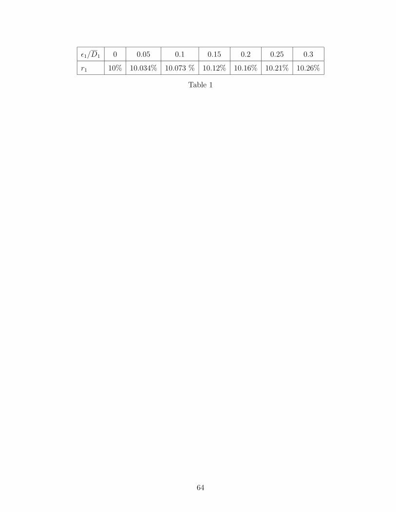
ε1/D1 0 0.05 0.1 0.15 0.2 0.25 0.3

r1 10% 10.034% 10.073 % 10.12% 10.16% 10.21% 10.26%

Table 1

64

ε1/D1 0 0.05 0.1 0.15 0.2 0.25 0.3

t1 0 6.6 9.1 10.9 12.8 13.6 14.6

V1 0.0381 0.0360 0.0352 0.0346 0.0342 0.0338 0.0334

Reduction 0 5.40% 7.50% 9.03% 10.28% 11.34% 12.26%

Table 2

65