An Analysis of the Principal-Agent Problem · Econometrica, Vol. 51, No. 1 (January, 1983) AN...
40
An Analysis of the Principal-Agent Problem Author(s): Sanford J. Grossman and Oliver D. Hart Source: Econometrica, Vol. 51, No. 1 (Jan., 1983), pp. 7-45 Published by: The Econometric Society Stable URL: http://www.jstor.org/stable/1912246 Accessed: 07/12/2010 13:06 Your use of the JSTOR archive indicates your acceptance of JSTOR's Terms and Conditions of Use, available at http://www.jstor.org/page/info/about/policies/terms.jsp. JSTOR's Terms and Conditions of Use provides, in part, that unless you have obtained prior permission, you may not download an entire issue of a journal or multiple copies of articles, and you may use content in the JSTOR archive only for your personal, non-commercial use. Please contact the publisher regarding any further use of this work. Publisher contact information may be obtained at http://www.jstor.org/action/showPublisher?publisherCode=econosoc. Each copy of any part of a JSTOR transmission must contain the same copyright notice that appears on the screen or printed page of such transmission. JSTOR is a not-for-profit service that helps scholars, researchers, and students discover, use, and build upon a wide range of content in a trusted digital archive. We use information technology and tools to increase productivity and facilitate new forms of scholarship. For more information about JSTOR, please contact [email protected]. The Econometric Society is collaborating with JSTOR to digitize, preserve and extend access to Econometrica. http://www.jstor.org
Transcript of An Analysis of the Principal-Agent Problem · Econometrica, Vol. 51, No. 1 (January, 1983) AN...

An Analysis of the Principal-Agent ProblemAuthor(s): Sanford J. Grossman and Oliver D. HartSource: Econometrica, Vol. 51, No. 1 (Jan., 1983), pp. 7-45Published by: The Econometric SocietyStable URL: http://www.jstor.org/stable/1912246Accessed: 07/12/2010 13:06
Your use of the JSTOR archive indicates your acceptance of JSTOR's Terms and Conditions of Use, available athttp://www.jstor.org/page/info/about/policies/terms.jsp. JSTOR's Terms and Conditions of Use provides, in part, that unlessyou have obtained prior permission, you may not download an entire issue of a journal or multiple copies of articles, and youmay use content in the JSTOR archive only for your personal, non-commercial use.
Please contact the publisher regarding any further use of this work. Publisher contact information may be obtained athttp://www.jstor.org/action/showPublisher?publisherCode=econosoc.
Each copy of any part of a JSTOR transmission must contain the same copyright notice that appears on the screen or printedpage of such transmission.
JSTOR is a not-for-profit service that helps scholars, researchers, and students discover, use, and build upon a wide range ofcontent in a trusted digital archive. We use information technology and tools to increase productivity and facilitate new formsof scholarship. For more information about JSTOR, please contact [email protected].
The Econometric Society is collaborating with JSTOR to digitize, preserve and extend access to Econometrica.
http://www.jstor.org

Econometrica, Vol. 51, No. 1 (January, 1983)
AN ANALYSIS OF THE PRINCIPAL-AGENT PROBLEM
BY SANFORD J. GROSSMAN AND OLIVER D. HART'
Most analyses of the principal-agent problem assume that the principal chooses an incentive scheme to maximize expected utility subject to the agent's utility being at a stationary point. An important paper of Mirrlees has shown that this approach is generally invalid. We present an alternative procedure. If the agent's preferences over income lotteries are independent of action, we show that the optimal way of implementing an action by the agent can be found by solving a convex programming problem. We use this to characterize the optimal incentive scheme and to analyze the determinants of the seriousness of an incentive problem.
1. INTRODUCTION
IT HAS BEEN RECOGNIZED for some time that, in the presence of moral hazard, market allocations under uncertainty will not be unconstrained Pareto optimal (see Arrow [1], Pauly [13]). It is only relatively recently, however, that economists have begun to undertake a systematic analysis of the properties of the second- best allocations which will arise under these conditions. Much of this analysis has been concerned with what has become known as the principal-agent problem. Consider two individuals who operate in an uncertain environment and for whom risk sharing is desirable. Suppose that one of the individuals (known as the agent) is to take an action which the other individual (known as the principal) cannot observe. Assume that this action affects the total amount of consumption or money which is available to be divided between the two individuals. In general, the action which is optimal for the agent will depend on the extent of risk sharing between the principal and the agent. The question is: What is the optimal degree of risk sharing, given this dependence?
Particular applications of the principal-agent problem have been made to the case of an insurer who cannot observe the level of care taken by the person being insured; to the case of a landlord who cannot observe the input decision of a tenant farmer (sharecropping); and to the case of an owner of a firm who cannot observe the effort level of a manager or worker.2
Although considerable progress has been made in the recent literature towards understanding and solving the principal-agent problem (see, in particular, Harris and Raviv [6], Holmstrom [7], Mirrlees [10, 11, 12], Shavell [19, 20], as well as the other references in footnote 2), the mathematical approach which has been adopted in most of this literature is unsatisfactory. The procedure usually followed is to suppose that the principal chooses the risk-sharing contract, or incentive scheme, to maximize his expected utility subject to the constraints that
'Support from the U.K. Social Science Research Council and NSF Grant No. SOC70-13429 is gratefully acknowledged. We would like to thank Bengt Holmstrom, Mark Machina, Andreu Mas-Colell, and Jim Mirrlees for helpful comments.
2These and other applications are discussed in a number of recent papers. See, for example, Harris and Raviv [6], Holmstrom [7], Mirrlees [10, 11, 12], Radner [15], Ross [17], Rubinstein and Yaari [18], Shavell [19, 20], Spence and Zeckhauser [21], Stiglitz [22], and Zeckhauser [24].
7
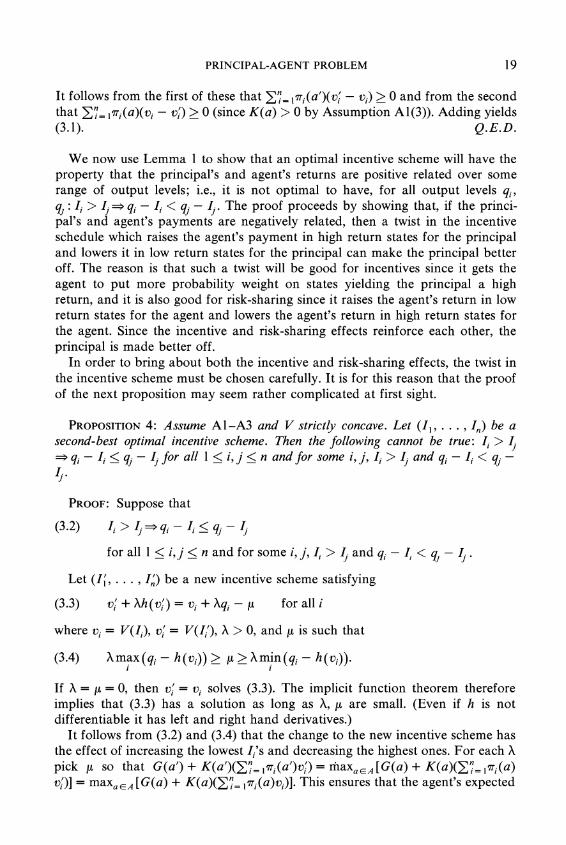
8 S. J. GROSSMAN AND 0. D. HART
a
A
_X~~~~~~~~~~~~3f
p > p2
D
P1
E
A
I I
For a given I the agent strictly prefers lower actions
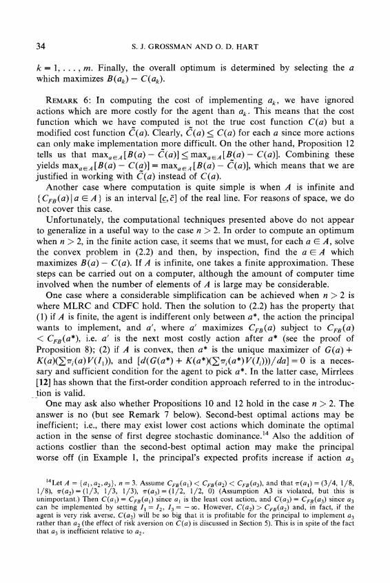
FIGURE 1.
(a) the agent's expected utility is no lower than some pre-specified level; (b) the agent's utility is at a stationary point, i.e., the agent satisfies his first-order conditions with respect to the choice of action. That is, the agent's second-order conditions (and the condition that the agent should be at a global rather than a local maximum) are ignored. Mirrlees [10], however, in an important paper, has shown that this procedure is generally invalid unless, at the optimum, the solution to the agent's maximum problem is unique. In the absence of uniqueness (and it is difficult to guarantee uniqueness in advance), the first-order conditions derived by the above procedure are not even necessary conditions for the optimality of the risk-sharing contract.3
3The reason for this can be seen quite easily in Figure 1 (we are grateful to Andreu Mas-Colell for suggesting the use of this figure). On the horizontal axis, I represents the agent's incentive scheme and on the vertical axis a represents the agent's action. The curve ABCDE is the locus of pairs of actions and incentive schemes which satisfy the agent's first order conditions, i.e., given I the agent's utility is at a stationary point. Of these points, only those lying on the segments AB and DE represent global maxima for the agent, e.g. given the incentive scheme I the agent's optimal action is at P', not at P2 or p3. Indifference curves-in terms of a and I-are drawn for the principal (C is on a higher curve than B). The true feasible set for the principal are the segments AB and DE and the optimal outcome for the principal is therefore B. However, B does not satisfy the first order conditions of the problem: maximize the principal's utility subject to (a, I) lying on ABCDE, i.e., subject to (a, I) satisfying the agent's first order conditions (the solution to this problem is at C). In other words, B does not satisfy the necessary conditions for optimality of the problem which has been studied in much of the literature. Note finally that perturbing Figure 1 slightly does not alter this conclusion.
PRINCIPAL-AGENT PROBLEM 9
The purpose of this paper is to develop a method for analyzing the principal- agent problem which avoids the difficulties of the "first-order condition" ap- proach.4 Our approach is to break the principal's problem up into a computation of the costs and benefits of the different actions taken by the agent. For each action, we consider the incentive scheme which minimizes the (expected) cost of getting the agent to choose that action. We show that, under the assumption that the agent's preferences over income lotteries are independent of the action he takes, this cost minimization problem is a fairly straightforward convex program- ming problem. An analysis of these convex problems as the agent's action varies yields a number of results about the form of the optimal incentive scheme. We will also be able to analyze what factors determine how serious a particular incentive problem is; i.e., how great the loss is to the principal from having to operate in a second-best situation where the agent's action cannot be observed relative to a first-best situation where it can be observed.
The assumption that the agent's preferences over income lotteries are indepen- dent of action is a strong one. Yet it seems a natural starting point for an analysis of the principal-agent problem. Special cases of this assumption occur when the agent's utility function is additively or multiplicatively separable in action and reward. One or other of these cases is typically assumed in most of the literature. In Section 6 we discuss briefly the prospects for the non-independence case.
In addition to providing greater rigor, the costs versus benefits approach also provides a clear separation of the two distinct roles the agent's output plays in the principal-agent problem. On the one hand, the agent's output contributes positively to the principal's consumption, so the principal desires a high output. On the other hand, the agent's output is a signal to the principal about the agent's level of effort. This informational role may be in conflict with the consumption role. For example, there may be a moderate output level which is achieved when the agent takes low effort levels and never occurs at other effort levels. If the agent is penalized whenever this moderate output occurs, then he is discouraged from taking these low effort actions. However, there may be lower output levels which have some chance of occurring regardless of the agent's action. To encourage the agent to take high effort levels, it is then optimal to pay the agent more in low output states than in moderate output states, even though the principal prefers moderate output levels to low output levels.
The dual role of output makes it difficult to obtain conditions which ensure even elementary properties of the incentive scheme, such as monotonicity. In Section 3, sufficient conditions for monotonicity are given. It is also shown in this section that a monotone likelihood ratio condition, which the "first-order condi- tion" approach suggests is a guarantee of monotonicity, must be strengthened once we take into account the possibility that the agent's action is not unique at the optimal incentive scheme.
The paper is organized as follows. In Section 2, we show how the principal's optimization problem can be decomposed into a costs versus benefits problem.
4Mirrlees [12] has identified a class of cases where the "first-order condition" approach is valid. We will consider this class in Section 3.

10 S. J. GROSSMAN AND 0. D. HART
In Section 3, we use our approach to analyze the monotonicity and progressivity of the optimal incentive scheme. In Section 4, we give a simple algorithm for computing an optimal incentive scheme when there are only two outcomes associated with the agent's actions. In Section 5, we analyze the effects of risk aversion and information quality on the incentive problem. Finally, in Section 6 we consider some extensions of the analysis.
2. STATEMENT OF THE PROBLEM
The application of the principal-agent problem that we will consider is to the case of the owner of a firm who delegates the running of the firm to a manager. The owner is the principal and the manager the agent. The owner is assumed not to be able to monitor the manager's actions. The owner does, however, observe the outcome of these actions, which we will take to be the firm's profit. It is assumed that the firm's profit depends on the manager's actions, but also on other factors which are outside the manager's control-we model these as a random component. Thus, in particular, if the firm does well, it will not generally be clear to the owner whether this is because the manager has worked well or whether it is because he has been lucky.5
We will simplify matters by assuming that there are only finitely many possible gross profit levels for the firm, denoted ql, . . . , qn, where q1 < q2 < . . . < qn. We will assume that the principal is interested only in the firm's net profit, i.e. gross profit minus the payment to the manager. We will also assume that the principal is risk neutral-our methods of analysis can, however, be applied to the case where the principal is risk averse (see Remark 3 and Section 6).
Let A be the set of actions available to the manager. We will assume that A is a non-empty, compact subset of a finite dimensional Euclidean space. Let S = { x E R I x > 0, En=1 7Xi = 1 }. We assume that there is a continuous function 7T: A -* S, where 7T(a) = (wj(a), ... , wn(a)) gives the probabilities of the n out- comes ql, . . . , qn if action a is selected. It is assumed that, when the agent chooses a E A, he knows the probability function 7T but not the outcome which will result from his action. We assume that the agent has a von Neumann- Morgenstern utility function U(a, I) which depends both on his action a and his remuneration I from the principal. We include a as an argument in order to capture the idea that the agent dislikes working hard, taking care, etc.
The crucial assumption that we will make about the form of U(a, I) is:
ASSUMPTION A1: U(a, I) can be written as G(a) + K(a) V(I), where (1) V is a real-valued, continuous, strictly increasing, concave function defined on some open interval I = (I, o) of the real line; (2) limI,, V(I) = - ox; (3) G, K are
5The assumption that the principal cannot monitor the agent's actions at all may in some cases be rather extreme. For a discussion of the implications of the existence of imperfect monitoring opportunities, see Harris and Raviv [6], Holmstrom [7] and Shavell [19, 20]. See also Remark 4 in Section 2.

PRINCIPAL-AGENT PROBLEM 11
real-valued, continuous functions defined on A and K is strictly positive; (4) for all a,, a2 E A and I
_ E, G(a,) + K(a1) V(I) ? G(a2)+ K(a2)V(I) => G(a) +
K(al) V(I) 2 G(a2) + K(a2) V(I).
In the above, we allow for the case I =- . The main part of Assumption Al has a simple ordinal interpretation. Assump-
tion Al implies that the agent's preferences over income lotteries are independent of his action (Assumption Al(1) tells us also that these preferences exhibit risk aversion). The converse can also be shown to be true: if the agent's preferences over income lotteries are independent of a, then U can be written as G(a) + K(a) V(I) for some functions G, K, V (for a proof, see Keeney [8]). Note that Assumption Al does not imply that the agent's preferences for action lotteries are independent of income. We will insist, however, that the agent's ranking over perfectly certain actions is independent of income-this is condition (4) of Assumption Al.
Note that if K(a) is not constant then (2) and (4) imply that V(I) must be bounded from above. Further if it is also the case that G(a) 0, then V(I) must be non-positive everywhere.
Two special cases of Assumption Al occur when K(a)= constant, i.e. U is additively separable in a and I, and when G(a) = 0, i.e. U is multiplicatively separable in a and I. In these cases the agent's preferences over action lotteries are independent of income, as well as preferences over income lotteries being independent of action.6
An interesting special case of multiplicative separability is when V(I)= -e- k, K(a) = eka and A is a subset of the real line. Then U(a,I) =
-e- k(-a); i.e., effort appears just as negative income. In the "first-best" situation where the principal can observe a, it is optimal for
him to pay the agent according to the action he chooses. Let U be the agent's reservation price, i.e. the expected level of utility he can achieve by working elsewhere, and let Qt = V(J) = {v v = V(I) for some I E }. We make the following assumption.
ASSUMPTION A2: [ U- G(a)]/K(a) E Q?t for all a E A.
DEFINITION: Let CFB A -> R be defined by CFB(a) = h([ U -G(a)]/K(a)), where h _ V- 1.
Here CFB stands for first-best cost. CFB(a) is simply the agent's reservation price for picking action a. To get the agent to pick a E A in the first-best
6The converse is also true: if preferences over action lotteries are independent of income as well as preferences over income lotteries being independent of action, then U is additively or multiplicatively separable (see Keeney [8] or Pollak [14]).
12 S. J. GROSSMAN AND 0. D. HART
situation, the principal will offer him the following contract: I will pay you CFB(a) if you choose a and I otherwise, where I is very close to I.
DEFINITION: Let B: A - R be defined by B(a) = I7T1(a)q1. B(a) is the expected benefit to the principal from getting the agent to pick a.
DEFINITION: A first-best optimal action is one which maximizes B(a) -
CFB(a) on A.
The function CFB induces a complete ordering on A: a a' if and only if CFB(a) ? CFB(a'). For obvious reasons we will refer to actions with higher CFB(a)'s as costlier actions. It is easy to show, in view of Assumption A1(4), that CFB(a) ? CFB(a') =- G(a) + K(a)v < G(a') + K(a')v for all v E Qt1 G(a) + K(a)v < G(a') + K(a')v for some v E Qt. This in turn implies that the ordering > is independent of U. In the second-best situation where a is not observed by the principal, it is not possible to make the agent's remuneration depend on a. Instead, the principal will pay the agent according to the outcome of his action, i.e. according to the firm's profit. An incentive scheme is therefore an n- dimensional vector I = (II , I2' ... . In) & In, where Ii is the agent's remuneration in the event that the firm's profit is q*. Given the incentive scheme I, the agent will choose a E A to maximize En= 17Tj(a) U(a, Ii).
We will assume that the principal knows the agent's utility function U(a, I), the set A and the function 7 :A -S. In other words, the principal is fully informed about the agent and about the firm's production possibilities. The incentive problem which we will study therefore arises entirely because the principal cannot monitor the agent's actions.7
The principal's problem can be described as follows. Let F be the set of pairs of incentive schemes I* and actions a* such that, under I*, the agent will be willing to work for the principal and will find it optimal to choose a*, i.e. maxa EAn Ii (a) U(a,IP) = En= 17j(a*)U(a*,PI*)> U. Then the principal chooses (I, a) E F to maximize En= I7Ti(a)(qi - I). It simplifies matter considera- bly if we break this problem up into two parts. We consider first, given that the principal wishes to implement a*, the least cost way of achieving this. We then consider which a* should be implemented. Thus, to begin, suppose that the principal wishes the agent to pick a particular action a* E A. To find the least (expected) cost way of achieving this, the principal must solve the following
7This distinguishes our study from the literature on incentive compatibility; see, e.g., the recent Review of Economic Studies symposium [16]. The incentive compatibility literature has been con- cerned with incentive problems arising from differences in information between individuals rather than with those arising from monitoring problems. In cases of differential information, there is a role for an exchange of information through messages, whereas in the model we study messages would serve no purpose.

PRINCIPAL-AGENT PROBLEM 13
problem:
n
(2.1) Choose II, ... , In to minimize W 7(a*)Ii i = 1
n
subject to W 71(a*) U(a*, Ii ) ? U, i = 1
n n
7 Ti(a*) U(a*, Ii) ? 7Ti (a) U(a, Ii) for all a E A, ___ i=l1
Ii EJ for all i.
This problem can be simplified considerably in view of Assumption Al. It will be convenient to regard vI = V(II), . . . , vn = V(In) as the principal's control variables. Recall that Qt = V(J) = { v v = V(I) for some I E f }. By Assumption Al, Qt is an interval of the real line (-oo,). Thus we may rewrite (2.1) as follows:
n
(2.2) Choose v, ... , vn to minimize W 7(a*)h(vi)
subject to G(a*) + K(a*) 7Ti(a*)1 2 G(a) + K(a)( 7Ti(a)vi)
for all a E A,
G(a*) + kK=1 a() ) (a) ,
vi et foralli,
where h V 1. The important point to realize is that the constraints in (2.2) are linear in the
vj's. Furthermore, V concave implies h convex, and so the objective function is convex in the vi's. Thus (2.2) is a rather simple optimization problem: minimize a convex function subject to (a possibly infinite number of) linear constraints. In particular, when A is a finite set, the Kuhn-Tucker theorem yields necessary and sufficient conditions for optimality. These will be analyzed later.
It is important to realize that, in the absence of Assumption Al, it is not generally possible to convert (2.1) into a convex problem in this way.
DEFINITION: If I = (II, ... , In) satisfies the constraints in (2.1) or v =
(vl, . .. , vn) satisfies the constraints in (2.2), we will say that I or v implements action a*. (We are assuming here that if the agent is indifferent between two actions, he will choose the one preferred by the principal.)
14 S. J. GROSSMAN AND 0. D. HART
Consider the set of v's which implement a*. For some a*, this set may be empty, in which case action a* cannot be implemented by the principal at any cost. If the set is non-empty, then, since h is convex,
n n U - UG(a*) 1 2 i(a*)vi) 2 h K(a*)
by (2.2), and so the principal's objective function is bounded below on this set. Let C(a*) be the greatest lower bound of En.=17Ti(a*)h(vi) on this set.
DEFINITION: Let C(a*) = inf { En= 17Ti (a *)h (vi) I v = (v 1, ... , vn) implements a*} if the constraint set in (2.2) is non-empty. In the case where the constraint set of (2.2) is empty, write C(a*) = ox. This defines the second-best cost function C: A -* Ru { o.
The above constitutes the first step(s) of the principal's optimization problem: for each a E A, compute C(a). The second step is to choose which action to implement, i.e. to choose a E A to maximize B(a) - C(a). This second problem will not generally be a convex problem. This is because even if B (a) is concave in a, C(a) will not generally be convex. Fortunately, a significant amount of information about the form of the optimal incentive scheme can be obtained by studying the first step alone.
DEFINITION: A second-best optimal action a is one which maximizes B(a) -
C(a) on A. A second-best optimal incentive scheme I is one that implements a second-best optimal action a at least expected cost, i.e. En=l7i( = c(a).
Note that for a second-best optimal incentive scheme to exist, the greatest lower bound in the definition of C(a) must actually be achieved. In order to establish the existence of a second-best optimal action and a second-best optimal incentive scheme, we need a further assumption.
ASSUMPTION A3: For all a E A and i = I, ... , n, 7Ti(a) > 0.
Since there are only finitely many possible profit levels, Assumption A3 implies that 7Ti(a) is bounded away from zero. Hence Assumption A3 rules out cases studied by Mirrlees [12] in which an optimum can be approached but not achieved by imposing higher and higher penalties on the agent which occur with smaller and smaller probability if the agent chooses the right action.
PROPOSITION 1: Assume A1-A3. Then there exists a second-best optimal action a and a second-best optimal incentive scheme I.

PRINCIPAL-AGENT PROBLEM 15
PROOF: It is helpful to split the proof up into two parts. Consider first the case where V is linear. Then it is easy to see that the principal can do as well in the second-best as in the first-best where the agent can be monitored. For let a* maximize B(a) - CFB(a) on A. Let the principal offer the agent the incentive scheme Ii = qi- t, where t = B(a*) - CFB(a*). Then the principal's profit will be B(a*) - CFB(a*) whatever the agent does. On the other hand, by picking a = a*, the agent can obtain expected utility U. Hence Proposition 1 certainly holds when V is linear.
On the other hand, suppose V is not linear. We show first, that, if the constraint set is nonempty for an action a* E A, then problem (2.2) has a solution, i.e. Z7%1vj(a*)h(v1) achieves its greatest lower bound C(a*). Note that
zi = ITi(a*)vi is bounded below on the 6onstraint set of (2.2). It therefore follows from a result of Bertsekas [2] that unbounded sequences in the constraint set make Zn=7 1(a*)h(v1) tend to infinity (roughly because the variance of the
vj-oo while their mean is bounded below, and h is convex and nonlinear- Assumption A3 is important here). Hence, we can artificially bound the con- straint set. Since the constraint set is closed, the existence of a minimum therefore follows from Weierstrass' theorem.
We show next that C(a) is a lower semicontinuous function of a. If A is finite, then any function defined on A is continuous and hence lower semicontinuous. Assume therefore that A is not finite. Let (ar) be a sequence of points in A converging to a. Assume without loss of generality (w.l.o.g.) that C(ar) -* k. Then, if k = ox, we certainly have C(a) < limrO C(ar). Suppose therefore that k < ox. Let (I, ... , In,) be the solution to (2.1) when a* = ar. Then Bertsekas' result together with Assumption A3 shows that the sequence ((IK, . .. , In)) is bounded (otherwise C(ar) -x oo). Let (II, . . . , In) be a limit point. Then clearly (II, . . . , In) implements a and so C(a) < Eni=17 i(a)Ij = limrO C(ar). This proves lower semicontinuity.
Given that C(a) is lower semicontinuous and A is compact, it follows from Weierstrass' theorem that maxa EA[B(a) - C(a)] has a solution, as long as C(a) is finite for some a E A. To prove this last part, we show that C(a*) = CFB(a*) if a* minimizes CFB(a) on A. To see this, note that the a* which minimizes CFB(a) can be implemented by setting Ii = CFB(a*) for all i.
We have thus established the existence of a second-best optimal action, a, when V is nonlinear. Since we have also shown that (2.2) has a solution as long as the constraint set is non-empty and V is nonlinear, this establishes the existence of a second-best optimal incentive scheme. Q.E.D.
It is interesting to ask whether the constraint that the agent's expected utility be greater than or equal to U is binding at a second-best optimum. The answer is no in general, i.e. for incentive reasons it may pay the principal to choose an incentive scheme which gives the agent an expected utility in excess of U. One case where this will not happen is when the agent's utility function is additively or multiplicatively separable in action and reward:

16 S. J. GROSSMAN AND 0. D. HART
PROPOSITION 2: Assume Al, A2, and either K(a) is a constant function on A or G(a) = 0 for all a E A. Let a' be a second-best optimal action and I a second-best optimal incentive scheme which implements a. Then a =r a(I) U(a,Ii)= U.
PROOF: Suppose not. Write v = V(I,). Then G( ) + K aa vi> U in (2.2). But it is clear that the principal's costs can be reduced and all the constraints of (2.2) will still be satisfied if we replace vi by (VI - E) for all i in the additively separable case and by vj(1 + e) for all i in the multiplicatively separable case where e > 0 is small (note that in the multiplicatively separable case, it follows from (2)-(4) of Assumption Al that V(I) < 0 for all I E 4, and so vI < 0). In other words, a can be implemented at lower expected cost, which contradicts the fact that we are at a second-best optimum. Q.E.D.
REMARK 1: The proof of Proposition 1 establishes that C(a*) = CFB(a*) if a* minimizes CFB(a) on A. This is a reflection of the fact that there is no trade-off between risk sharing and incentives when the action to be implemented is a cost-minimizing one (i.e. involves the agent in minimum "effort").
REMARK 2: In general, there may be more than one second-best optimal action and more than one second-best optimal incentive scheme. It is clear from (2.2), however, that, if V is strictly concave, there is a unique second-best optimal incentive scheme which implements any particular second-best optimal action.
DEFINITION: Let L = maxaEA(B(a) - CFB(a))- SUpaEA(B(a) - C(a)) be the difference between the principal's expected profit in the first-best and second- best situations.
L represents the loss which the principal incurs as a result of being unable to observe the agent's action (we write sup(B(a) - C(a)) rather than max(B(a) -
C(a)) to cover cases where the assumptions of Proposition 1 do not hold). Proposition 3 shows that, while there are some special cases in which L = 0, in general L > 0.
PROPOSITION 3: Assume Al and A2. Then: (1) C(a) > CFB(a) for all a E A, which implies that L > 0. (2) If V is linear, L = 0. (3) If there exists a first-best optimal action a* E A satisfying: for each i, 7Ti(a*) > O X 7T,(a) = O for all a E A, a # a*, then L = 0. (4) If A is a finite set and there is a first-best optimal action a* which satisfies: for some i, 7Tj(a*) = 0 and 7Tj(a) > 0 for all a E A, a # a*, then L = 0. (5) If there is a first-best optimal action a* E A which minimizes CFB (a) on A, L = 0. (6) If Assumption A3 holds, every maximizer a of B(a) - CFB(a) on A satisfies CFB (a) > mina EA CFB (a), and V is strictly concave, then L > 0.
PROOF: (1) is obvious since anything which is second-best feasible is also first-best feasible. (2) follows from the first part of the proof of Proposition 1. (5) follows from the proof of Proposition 1 (see also Remark 1). (3) and (4) follow from the fact that a* can be implemented by offering the agent Ii = CFB (a*) for those i such that 7Ti(a*) > 0 and I close to I otherwise.

PRINCIPAL-AGENT PROBLEM 17
To prove (6), note that, if V is strictly concave,
n
G(a*) + K(a*) 7Ti(a*) V(Ii) > U i=l
implies
n
C(a*) = 7Ti(a*)h(V(Ii)) i=l1
> h ( 7Ti(a*) V(Ii)) 2 h ((_ U-G(a*))/K(a*))
CFB (a*)
unless Ii = constant with probability 1. But, since 7i(a*) > 0 for all i, Ii =
constant with probability 1 => Ii is independent of i. However, in this case, the constraints of problem (2.2) imply that CFB (a) is minimized at a*. Q.E.D.
Most of Proposition 3 is well known. Proposition 3(2) and (6) can be under- stood as follows. In the first-best situation, if the agent is strictly risk averse, the principal bears all the risk and the agent bears none. In the second best situation, this is generally undesirable. For if the agent is completely protected from risk, then he has no incentive to work hard; i.e., he will choose a E A to minimize CFB(a). Hence the second-best situation is strictly worse from a welfare point of view than the first-best situation. The exception is when the agent is risk neutral, in which case it is optimal both from a risk sharing and an incentive point of view for him to bear all the risk, or when the first-best optimal action is cost minimizing.
In the case of Proposition 3(3) and 3(4), a scheme in which the agent is penalized very heavily if certain outcomes occur can be used to achieve the first best. This relates to results obtained in Mirrlees [12].
REMARK 3: We have assumed that the principal is risk neutral. Our analysis generalizes to the case where the principal is risk averse, however. In this case, instead of choosing v to minimize Z7Ti(a*)h(v1) in problem (2.2), we choose v to maximize E7Ti(a*) Up (q - h(vi)), where Up is the principal's utility function. Note that (2.2) is still a convex problem. Although we can no longer analyze costs and benefits separately, we can, for each a* E A, define a net benefit function maxv2vZi(a*) Up (q - h(vi)). An optimal action for the principal is now one that maximizes net benefits. See also Section 6 on this.
REMARK 4: We have taken the outcomes observed by the principal to be profit levels. Our analysis generalizes, however, to the case where the outcomes are more complicated objects, such as vectors of profits, sales, etc., or to the case where profits are not observed at all but something else is (see, e.g., Mirrlees [11]). The important point to realize is that profit does not appear in the cost

18 S. J. GROSSMAN AND 0. D. HART
minimization problem (2.1) or (2.2). Thus, if the principal observes the realiza- tions of a signal 0, then Ii refers to the payment to the agent when 0 i . Let C(a, 0) be the cost of implementing a when the information structure is 0 (e.g. if 0 reveals a exactly, then C(a, 0) = CFB(a)). Note that if the distribution of output is generated by a production function f(a, w), such that the marginal distribu- tion of w is independent of the information structure, then B (a) = Ef(a, w-) = E [E [f(a, w-) I 01]] is independent of the information structure, given a. It follows that the effect of changes in the information structure is summarized by the way that C(a, 0) changes when the information structure changes. As will be seen in Section 5, this is quite easy to analyze.
3. SOME CHARACTERISTICS OF OPTIMAL INCENTIVE 'CHEMES
It is of interest to know whether the optimal incentive scheme is monotone increasing (i.e., whether the agent is paid more when a higher output is observed) and whether the scheme is progressive (i.e., whether the marginal benefit to the agent of increased output is decreasing in output). These questions are quite difficult to answer because of the informational role of output. As we noted in the introduction, the agent may be given a low income at intermediate levels of output in order to discourage particular effort levels. Nevertheless, some general results about the shape of optimal schemes can be established. We begin with the following lemma.
LEMMA 1: Assume A1-A3. Let (I)'=1, (Ii')= I be incentive schemes which cause a and a' to be optimal choices for the agent, respectively, and minimize the respective costs (i.e. (2.1) or (2.2) is solved). Let vi = V(I) and vi' = V(Ii'). Then, if G(a) + K(a)(En= 1I1i(a)vi) = G(a') + K(a')( i= I 7T"(a')vt'), i.e. the agent's ex- pected utility is the same under both schemes, we must have
(3.1) [7Tj (a) )- gi(a) ] (i' -vi) > O.
PROOF: From (2.2) and the assumption that the agent's expected utility is the same, we have
G(a') + K(a')( 7i(a')vi) < G(a) + K(a)( q rTi(a) v)
= G(a') + K(a ) Ti(a vi
G(a) + K(a)( 7i(a)vi') < G(a') + K(a')( 2rTi(a')v')
= G(a) + K(a)( g vri(a)vt).
PRINCIPAL-AGENT PROBLEM 19
It follows from the first of these that I qrTi(a')(v' - vi) > 0 and from the second that I gi=r(a)(vi - v') > 0 (since K(a) > 0 by Assumption A1(3)). Adding yields (3.1). Q.E.D.
We now use Lemma 1 to show that an optimal incentive scheme will have the property that the principal's and agent's returns are positive related over some range of output levels; i.e., it is not optimal to have, for all output levels q*, qj: I, > Ij X - I, < qj- I. The proof proceeds by showing that, if the princi- pal's and agent's payments are negatively related, then a twist in the incentive schedule which raises the agent's payment in high return states for the principal and lowers it in low return states for the principal can make the principal better off. The reason is that such a twist will be good for incentives since it gets the agent to put more probability weight on states yielding the principal a high return, and it is also good for risk-sharing since it raises the agent's return in low return states for the agent and lowers the agent's return in high return states for the agent. Since the incentive and risk-sharing effects reinforce each other, the principal is made better off.
In order to bring about both the incentive and risk-sharing effects, the twist in the incentive scheme must be chosen carefully. It is for this reason that the proof of the next proposition may seem rather complicated at first sight.
PROPOSITION 4: Assume A1-A3 and V strictly concave. Let (II,... , In) be a second-best optimal incentive scheme. Then the following cannot be true: Ii > Ij
q- I< qj- Ifor all 1 <i,j< n and for some i,j, I,>I. and q, - I,< q1- Ii I .
PROOF: Suppose that
(3.2) I, > Ij X q-I, < q1 -Ij
for all 1< i ,< n and for some i,j, I, > Ij and q* - I, < qj- Ij.
Let (I', . . ., In) be a new incentive scheme satisfying
(3.3) v'+Xh(vv')=v1+Xq1- i foralli
where vi = V(I), vi' = V(Ii'), X > 0, and ti is such that
(3.4) Xmax(q1 - h(vi)) > ? > Xmin(q1 - h(vi)). 1 1
If X = y = 0, then vi' = vi solves (3.3). The implicit function theorem therefore implies that (3.3) has a solution as long as X, y are small. (Even if h is not differentiable it has left and right hand derivatives.)
It follows from (3.2) and (3.4) that the change to the new incentive scheme has the effect of increasing the lowest Ii's and decreasing the highest ones. For each X pick ti so that G(a') + K(a')( I7. T1(a')v1') = lfaxaesA[G(a) + K(a)(En= ITi (a) vi')] = maxaEA[G(a) + K(a)(En=. Ig(a)v1)]. This ensures that the agent's expected

20 S. J. GROSSMAN AND 0. D. HART
utility remains the same. We now show that the principal's expected profit is higher under the new incentive scheme than under the old, which contradicts the optimality of (II, * . , IJ)
Substituting (3.1) of Lemma 1 into (3.3) yields:
i i(a')(qi -h (v')) > i T1(a)(qi-h (v-))
If we can show that E wi(a)h(v1') < Z7Ti(a)h(vj), it will follow that
i (a')(qi - h(v')) >E 7Ti(a)(qi - h(v1)),
i.e., the principal is better off. To see that E wi(a)h(v1') < Ewi(a)h(vi), note that
7T1i(a)(h (vi) - h (v')) > E 7Ti(a)h'(v')(vi - v)
by the convexity of h (here h' is the right-hand derivative if h is not differentia- ble). It suffices therefore to show that the latter expression is positive. By (3.3),
ETi (a) h'(vi')V- vi') = v 7Ti(a)h (vi)(h(vi)-Xq + I
Suppose that this is nonpositive for small X. Divide by X and let X -> 0. Assuming without loss of generality ti/X converges to i (we allow i infinite) and that h'(v') converges to h', and using the fact that v' - vi, we get
(3.5) 7Ti (a)h1'(h(vi) - q1 + i) < 0.
However, from the fact that h'(v') is nondecreasing in vi' and vi' - vi, h'(v1') hi it follows that vi > vj = h' > hj. Hence by (3.2) h' and (h(vi) - q1) are similarly ordered in the sense of Hardy, Littlewood, and Polya [5]; i.e., as one moves up so does the other. Therefore, by Hardy, Littlewood, and Polya [5, p. 43], h' and (h (vi) - q1) are positively correlated, i.e.,
(3.6) 27Ti (a) h'(h (vi) - q + A) > ( Ti(a)h/)(E Ti (a)(h (vi) - q + ii))
>0,
where the last inequality follows from the fact that (1) h' > 0; (2) G(a) + K(a) (7ri (a) v') < G (a') + K(a')(E, 71(a') v') = G (a) + K(a)(2 Ei(a)vi) (since the agent's expected utility stays constant), which implies that
lim (1 /X) E 7Ti (a)(vi - i)) > 0.
(3.6) contradicts (3.5). This proves that Zgr1(a)h(v1') < Z wi(a)h(vi), which establishes that the princi-
pal's expected profit is higher under (I', . . , I,) Contradiction. Q.E.D.
REMARK 5: Another way of expressing Proposition 4 is that there is no

PRINCIPAL-AGENT PROBLEM 21
permutation i1, . . ., in of the integers 1, . . . , n such that Ilkis nondecreasing in k, and (qiA - IiA) is nonincreasing in k, with Ilk < IIA+I, (qiA - IA) > (qiA+, -IiA+)
for some k. Note that there is an interesting contrast between Proposition 4 and results found in the literature on optimal risk sharing in the absence of moral hazard. In this literature (see Borch [4]), it is shown that (if the individuals are risk averse) it is optimal for the individuals' returns to be positively related over the whole range of outcomes, whereas here we are only able to show that this is true over some range of outcomes.
Proposition 4 may be used to establish the following result about the monoton- icity of the optimal incentive scheme.
PROPOSITION 5: Assume A1-A3 and V strictly concave. Let (II, ... , In) be a second-best optimal incentive scheme. Then (1) there exists 1 < i < n - 1 such that Ii < Ii+I, with strict inequality unless II =2= * =In; (2) there exists 1 < j < n-1 such that q. - Ij < q j+ I -
PROOF: (1) follows directly from Proposition 4. So does (2) once we rule out the case q1 - II = q2 - I2 = . = qn- In. We do this by a similar argument to that used in Proposition 4. Suppose that I is an optimal incentive scheme satisfying
(3.7) q1-II = q2-1I2 = qn-In = k
Then I, < I2 < . . . < In. Consider the new incentive scheme I' = (II + E, I2 + E, ... ., In-I + E,In - [E) where E > 0 and y is chosen so that maxaeA [G(a) + K(a)(Z'ii(a) V(Ij))] = maxA EA [G(a) + K(a)(Z'ii(a) V(I,))], i.e. the agent's ex- pected utility is kept constant. We show that the principal's expected profit is higher under I' than under I for small E. Suppose not. Then
7Ti(a')(4i - Ii') < Z7Ti(a)(q1 -
J) = k,
where a' (resp. a) is optimal for the agent under I' (resp. I). Substituting for I' yields
-(1 - Tn (a'))E + wn(a') LE < 0.
Take limits as E - 0. Without loss of generality a' - a'. Hence we have
(3.8) - (1 - qTn(A)) + Tn( A) tu < 0.
Now since a' is an optimal action for the agent under I', it follows by uppersemicontinuity that a is optimal under I. Hence we have
G(a) + K(a)( a7T1(a) V(1' )) < G(a') + K(a') Ti(a) V(Ii'))
= G(a) + ( A i(A) V(ji
Hence ar1( )( V(L) -V(IJ')) > 0. Using the concavity of V and taking limits as

22 S. J. GROSSMAN AND 0. D. HART
E - 0, we get
n-I
E ,ia V I -R a) V, (In
But since V'(Ii) is decreasing in i, this contradicts (3.8). (If V is not differentiable, V' denotes the right-hand derivative.)
This proves that the principal does better under I' than under I. Hence we have ruled out the case q- = * **= - In. This establishes Proposition 5.
Q.E.D.
Proposition 5 says that it is not optimal for the agent's marginal reward as a function of income to be negative everywhere or to be greater than or equal to one everywhere.8 However, the proposition does allow for the possibility that either of these conditions can hold over some interval. To see when this may occur, it is useful to consider in more detail the case where A is a finite set. When A is finite, we can use the Kuhn-Tucker conditions for problem (2.2) to characterize the optimum. If Assumption A3 holds and h is differentiable, these yield:
(3.9) h'(v1) = lX + E Yj K(a*) -E [t ( a) I for ) ) [ aj EA Jaj EA 7Tj(a*)) frl, L aj =,P+ a* aj =,,+aa*
where X, ( y>) are nonnegative Lagrange multipliers and yj > 0 only if the agent is indifferent between a* and aj at the optimum. The following proposition states that yj > 0 for at least one action which is less costly than a*. This implies that at an optimum the agent must be indifferent between at least two actions (unless a* is the least costly action, i.e. where there is no incentive problem).
PROPOSITION 6: Assume A1-A3 and A finite. Suppose that (2.2) has a solution for a* E A. Then if CFB (a*) > mina eA CFB (a), this solution will have the property that G(a*) + K(a*)( >I rj(a*)vj) = G(aj) + K(aj)(n=ITi1 (aj) vi) for some a. E A with CFB(a1) < CFB(a*). Furthermore, if V is strictly concave and differentiable, the Lagrange multiplier ,uj will be strictly positive for some aj with CFB(aj) < CFB(a*).
PROOF: Suppose that the agent strictly prefers a* to all actions less costly than a* at the solution. Then, since (2.2) is a convex problem, we can drop all the constraints in (2.2) which refer to less costly actions without affecting the
8Among other things, Proposition 5 shows that it is not optimal to have ql -II = q2- I2= = q- I,. This result has also been established by Shavell [20] under stronger assumptions.

PRINCIPAL-AGENT PROBLEM 23
solution. In other words, we can substitute A' = (a E A I a is at least as costly as a*} for A in (2.2) and the solution will not change. But since a* is now the least costly action, we know from the proof of Proposition 1 that it is optimal to set Ii = Ij for all i, j. However, Ii = Ij is not optimal for the original problem since, under these conditions, the agent will pick an a which minimizes CFB(a), and by assumption CFB (a*) > mina EA CFB (a). Contradiction.
That Ai > 0 follows from the fact that if all the yj = 0, then h'(vi) is the same for all i, which implies that I1 = .. = In; however, this means that the agent will choose a cost-minimizing action, contradicting CFB(a*) > minaEA CFB(a).
Q.E.D.
It should be noted that Proposition 6 depends strongly on the assumption that A is finite.
The simplest case occurs when yj > 0 for just one aj with CFB(aj) < CFB(a*)
(this will be true in particular if A contains only two actions). In this case, we can rewrite (3.9) as
(3.10) h'(vi) = (X + tt)K(a*) - ttK(aj) -( a* .
We see that what determines vi, and hence Ii, in this case is the relative likelihood that the outcome q = qi results from a1 rather than from a*. In particular, since h convex =X h' nondecreasing in vi, a sufficient condition for the optimal incentive scheme to be nondecreasing everywhere, i.e. I, < '2 < ? ..
<In, is that gi(aj)/1i(a*) is nonincreasing in i, i.e. the relative likelihood that a = a1 rather than a = a* produces the outcome q = qi is lower the better is the outcome i.
This observation has led some to suggest that the following is a sufficient conditon for the incentive scheme to be nondecreasing.
MONOTONE LIKELIHOOD RATIO CONDITION (MLRC): Assume A3. Then
MLRC holds if, given a, a' E A, CFB (a') < CFB (a) implies that 7Ti (a')/7Ti(a) is nonincreasing in i.
It should be noted that the "first-order condition" approach described in the introduction, which is based on the assumption that the agent is indifferent between a and a + da at an optimum, does yield MLRC as a sufficient condition for monotonicity.9 We now show, however, that, once we take into account the possibility that the agent may be indifferent between several actions at an
9See Mirrlees [11] or Holmstrom [7]. Milgrom [9] has shown that MLRC, as stated here, implies the differential version of the monotone likelihood condition which is to be found in Mirrlees [11] or Holmstrom [7].
24 S. J. GROSSMAN AND 0. D. HART
optimum, i.e. yj > 0 for more than one aj, MLRC does not guarantee monotonic- ity.
EXAMPLE 1: A = {a1, a2, a3}, n = 3. 7T(a1) = 23,, 2 ), T(a2)=(-}43 3), 7T(a3)
= ( ll2 4, 2 ). Assume additive separability with G(a1) =0, G(a2) =-( V
+ 7/4), G(a3)=-17/4, V(I) = (3I)1/3 (i.e. h(v) = 4v3),K(a) - and
U = 2 + 1 7/4. Note that MLRC is satisfied here.10 We compute C(a1), C(a2), C(a3). Obviously, C(a,) = CFB(al)= 4(U -G(a,))
= 0.033. To compute C(a2), we use the first-order conditions (3.9). These are
v2~~~~~~-2
V1 =-l + 34 12,
V2 4 A I y 4 A2,
V3=+ 4 Al- 21
plus the complementary slackness conditions. These equations are solved by setting X = 4, 1 = 2, A2 = 1. This yields v, = 0, v2 = , V3 = 7/4, and the agent is then indifferent between a,, a2, and a3:
3v +lv2+ v3+ G(a) =4 v+2 + 2 V3 + G(a2)
= 12 V + 4V2 + 233 + G(a3) = U.
Since the first-order conditions are necessary and sufficient, we may conclude that C(a2)= (3v+ V3+ v3)= 0.571.
Note that the incentive scheme which implements a2, I= 0, I2 = 23/2, I3 = 3 ( )3/2, is not nondecreasing.
Observe that C(a3) > CFB(a3) = l(U - G(a3))3 = 0.635 > C(a2). Since C(a3) > C(a2) > C(a,), it is easy to show that we can find q1 < q2 < q3 such that B(a2) - C(a2) > max[B(a3) - C(a3), B(a,) - C(a,)]. But this means that it is optimal for the principal to get the agent to pick a2. Hence the optimal incentive scheme is as described above. It is not nondecreasing despite the satisfaction of MLRC.
The reason that monotonicity breaks down in Example 1 is because, at the optimum, the agent is indifferent between a2, the action to be implemented, a1 a less costly action, and a3 a more costly action. By MLRC gr (a1)fir(a2), gi(a2) /1,g(a3) are decreasing in i. However, Aj(7Tr(aj)f7Tw(a2)) + 2(qTi(a3)/i(a2)) need not be monotonic.
This observation suggests that one way to get monotonicity is to strengthen MLRC so that it holds for weighted combinations of actions as well as for the
'0The function V violates (2) of Assumption Al, but this is unimportant for the example.

PRINCIPAL-AGENT PROBLEM 25
basic actions themselves. In particular, suppose that
(3.11) given any finite subset { al, . . . , am } of A, a E A,
and nonnegative weights wl, ... ., Wm summing to 1,
it is the case that ( Wj7Ti(aj)/Ti(a))
is either nondecreasing in i or nonincreasing in i.
Then, by the first-order conditions (3.9),
(3.12) h'(v1) = X + j K(a*) - lAj K(aj) L 7j 7(aj)
aj EA aj EA aj EA
where
Wj = ttjK (aj)/ E hK(ah).
ah E A ah # a*
But, by (3.1 1), the right-hand side (RHS) of (3.12) is monotonic. Hence, the v,'s are either monotonically nondecreasing or nonincreasing. By Proposition 5, however, they cannot be nonincreasing; hence they are nondecreasing.
Unfortunately, (3.11) turns out to be a very strong condition. In fact, it is equivalent to the following spanning condition.
SPANNING CONDITION (SC): There exists T, 4' E S such that (1) for each aeA, EA (a)=X(a)47+(1-X(a))47' for some O<X(a)<1; (2) 7/Til'T is nonin- creasing in i.
That SC implies (3.11) is easy to see. We are grateful to Jim Mirrlees for pointing out and proving the converse.' 1
PROPOSITION 7: Assume Al-A3, V strictly concave and differentiable. Suppose that SC holds. Then a second-best optimal incentive scheme satisfies II < I2 < ? . .
< In.
PROOF: If A is finite, the argument following (3.12) establishes the result. To establish the result for the case A infinite, let a E A be a second-best optimal
l To prove the converse, define a < a' if ?r,(a')/Ir,(a) is nondecreasing in i. (3.11) implies that 5 is a complete pre-ordering on A. Furthermore, z is continuous. Since A is compact, there exist a, a E A such that a < a < a for all a E A. Given a E A, consider X(?T, ()/r, (a)) + (1 -X)(Q,(a)/r, (a)). When A = 1, this is nondecreasing in i, and when A = 0, it is nonincreasing in i. Furthermore, (3.11) implies that it is monotonic in i for all 0 < A < 1. It follows by continuity that it is independent of i for some 0<A< 1.

26 S. J. GROSSMAN AND 0. D. HART
action and let I be the second-best optimal incentive scheme which implements it. By Remark 2 of Section 2, I is unique. Let Ar be a finite subset of A containing a such that the Euclidean distance between Ar and A is less than (1/r). Let Ir be the second-best optimal incentive scheme which implements a when the agent is restricted to choosing from Ar. From Proposition 7 for the finite A case, we know that Ir is nondecreasing. Take limits as r -4 0. It is straightforward to show that Ir - I. It follows that I is nondecreasing. Q.E.D.
An alternative sufficient condition for monotonicity may be found in the work of Mirrlees [12], who establishes a similar result to Proposition 8 below. For each a E A, let F(a) = (7T,(a), 7Tw(a) + 7T2(a), . .. , 7TI(a) + * * * + w"j(a)). In the follow- ing proposition, the notation F(a) > F'(a) is used to mean Fi(a) > F,'(a) for all
= 1, ... , n.
CONCAVITY OF DISTRIBUTION FUNCTION CONDITION (CDFC): CDFC holds if a,a',a" EA, and
(U -G(a) ) - (U G(a/)) + (1 - )(U G(a/))
( K(a) ) ( K(a') )( K(a")) O<X< 1,
imply that F(a) < XF(a') + (1 - X)F(a").
PROPOSITION 8: Assume A1-A3, V strictly concave and differentiable. Assume also that U is additively or multiplicatively separable, i.e., either G(a) 0_ or K(a) constant. Suppose that MLRC and CDFC hold. Then a second-best optimal incentive scheme (II, . .. , In) satisfies I, < I2< ? .. < In.
PROOF: Assume first that A is finite. Let a* maximize B(a) - C(a). Let A' = {a E A I CFB(a) < CFB(a*)}. Consider the cost minimizing way of getting the agent to pick a* given that he can choose only from A'. It is clear from (3.9) that, since qTi(aj)/qTi(a*) is nonincreasing in i by MLRC, the incentive scheme (II, ... , In) is nondecreasing. We will be home if we can show that (II, .. ., In) is optimal when A' is replaced by A. Since adding actions cannot reduce the cost of implementing a*, all we have to do is to show that (II, . .. , In) continues to implement a*, i.e. there does not exist a", CFB(a") > CFB(a*), such that
(3.13) G(a") + K(a")(w,E 7Tj(a")vj) > G(a*) + K(a*)(EqTi (a*)vi).
However, we know from Propositions 2 and 6 that
(3.14) G(a*) + K(a*)(Z7Tj(a*)vj) = G(a') + K(a')(ET7Ti(a')v1) = U
for some a' with CFB(a') < CFB(a*). Writing
G(a*) -( - G(a") + ( ) UK-G(a_)_ UK(a*) (UK(a") ) 1-A KUG(a/))

PRINCIPAL-AGENT PROBLEM 27
and using CDFC and the fact that vj < v2 < < v, we get
qTia* (i U -G(a))
> XZ7Tj(a")v1+ (1- X)(Xegn(a')v,) - ( -G(a*))
=X X27T(a")vi - K(U )
+ (l-X) E7Tj(a')vi - ( U-G(a')
But this contradicts (3.13) and (3.14). To prove the result for A finite, one again proceeds by way of finite approxi-
mation. Q.E.D.
To understand CDFC, consider, for each a E A, V(CFB(a)) =((U -G(a))
/K(a)). In utility terms V(CFB(a)) is a measure of the first-best cost of getting the agent to pick a. CDFC says that if a is a convex combination of a' and a" in terms of this measure of cost then the distribution function of outcomes corre- sponding to a dominates in the sense of first degree stochastic dominance the corresponding convex combination of the distribution functions corresponding to a' and a". It is worth noting that under the assumption of additive or multiplica- tive separability in Proposition 8, the X in the CDFC definition is independent of U.
So far we have considered only the monotonicity of the optimal incentive scheme. One would also like to know when the optimal incentive scheme is progressive, i.e. (II - i)/(q+I - qi) is nonincreasing in i, or regressive, i.e.
(I+j - i)/(qi+l - qi) is nondecreasing in i. To get results about this, one needs considerably stronger assumptions, as the following proposition indicates.
PROPOSITION 9: Assume Al-A3, V strictly concave and differentiable. Assume also that U is additively or multiplicatively separable, i.e., either G(a) 0_ or K(a) constant. Suppose that MLRC and CDFC hold and that (qi+I - qi) is independent of i, 1 < i < n - 1. Then a second-best optimal incentive scheme will be regressive (resp. progressive) if
(3.15) (1/ V'(I)) is concave (resp. convex) in I and a,a' E A,
CFB (a') < CFB (a), implies that (7Tj+ 1(a')/ rj+ 1(a)) - (7rj(a')/7Tj(a))
is nonincreasing (resp. nondecreasing) in i.
28 S. J. GROSSMAN AND 0. D. HART
PROOF: Assume first that A is finite. Let a* be a second-best optimal action. Let a' maximize CFB(a) subject to CFB(a) < CFB(a*), i.e. a' is the next most costly action after a*. Consider the cost minimizing way of implementing a* given that a' is the only other action that the agent can choose. Using the same concavity argument as in the proof of Proposition 8, we can show that the resulting incentive scheme (II, . .. , I) also implements a* when the agent can choose from all of A. Hence (I . . ., I) is an optimal incentive scheme.
By (3. 10),
V'(I ) = h'(vi) = (X + [t)K(a*) - [(a') (a *)
and so
1 - 1 - K(' ) i( TE?1(a*) _ 7r(a ) )
(3.15) now follows immediately. To prove the result for the A infinite case, one again proceeds by way of a finite approximation. Q.E.D.
Note that I/V' is linear if V=logI; is concave if V= -e', a >0, or V= I', 0 < a < 1; is convex if V = -I-, a > 1.
It should also be noted that Mirrlees [12] has shown that if CDFC holds, the "first-order condition" approach referred to in the introduction is valid. Thus Propositions 8 and 9 can also be proved by appealing to the characterization of an optimal incentive scheme to be found in much of the literature (see, e.g., Holmstrom [7] and Mirrlees [11]).
Let us summarize the results of this section. We have shown that an optimal incentive scheme will not be declining everywhere, but that only under quite strong assumptions (SC or MLRC plus concavity) will it be nondecreasing everywhere. We have also shown that it is not optimal for the agent's marginal remuneration for an extra pound of profit to exceed one everywhere, although it may exceed one sometimes. Finally, we have obtained sufficient conditions for the incentive scheme to be progressive or regressive.
The conclusion that only under strong assumptions will the optimal incentive scheme be monotonic may seem disappointing at first sight. One feels that monotonicity is a minimal requirement. This may not be the right reaction, however. There are many interesting situations where it is clear that the optimal scheme will not be monotonic. We have described one example in the introduc- tion. Another example is the following. Suppose that actions are two dimen- sional, with one dimension referring to how hard the agent works and the other dimension to how cautious he is-greater caution might lead to a lower variance of profit but also to a lower mean. The optimal action for the principal might involve the agent working fairly hard and also not being too cautious. The best

PRINCIPAL-AGENT PROBLEM 29
way to implement this may be to pay the agent high amounts for both very good outcomes (to encourage high effort) and very bad outcomes (to discourage excessive caution). This example seems far from pathological. In fact, one might argue that a number of real world incentive schemes operate in this way. In view of examples like this, the difficulty of finding general conditions guaranteeing monotonicity may become less surprising.12
In the next section, we show that considerably stronger results than those of this section can be proved for the case n = 2. We also provide a simple algorithm for computing optimal incentive schemes when n = 2.
4. THE CASE OF TWO OUTCOMES
When n = 2, we will refer to q, as the "bad" outcome and q2> q, as the "good" outcome. In this case, the agent's incentive scheme can be represented simply by a fixed payment w and a share of profits, s, where w + sq1 = II, w + sq2 = I2' i.e., s = (I2- Il)/(q2- q1). Proposition 5 of the last section shows that it is not optimal for Ii to be everywhere declining in qi. When n = 2, this means that s > 0.13 Similarly the proposition implies that s < 1 when n = 2. This has a number of interesting implications.
DEFINITION: Let n = 2. We say that a E A is efficient if there does not exist a' E A satisfying CFB(a') < CFB (a) and 7T2(a') > 7T2(a), with at least one strict inequality.
In other words, an action is efficient if the probability of a good outcome can only be increased by incurring greater cost.
PROPOSITION 10: Assume A1-A3 and V strictly concave. Let n = 2. Then every second-best optimal action is efficient.
PROOF: Let a be a second-best optimal action. Then a maximizes G(a) + K(a)
[7gI(a)v1 + 7g,(a)v2]. Suppose CFB(a') < CFB(a) and 7T2(a') > 7T2(a), with at least one strict inequality. Then, by the definition of CFB,
G(a) + K(a) V(CFB (a)) = U = G(a') + K(a) V(CFB (a'))
< G(a') + K(a) V(CFB (a))
12There are some cases where monotonicity may be a constraint on the optimal incentive scheme. An example is where the agent can always make a better outcome look like a worse outcome by reducing the firm's profits after the outcome has occurred. This case can be analyzed by adding the (linear) constraints v1 < v2 < . .< vn to the problem (2.2).
13Shavell [19] also proves that s > 0 when n = 2, but under stronger assumptions.

30 S. J. GROSSMAN AND 0. D. HART
since CFB(a') < CFB(a). Hence, by Assumption A1(4), G(a) + K(a)v < G(a') + K(a')v for all v E 9t. Therefore using the fact that v1 < v2 since s > 0, and the fact that 7T2(a') > 72(a), we have
G(a) + K(a)[7T,(a)v 2 + 72(a)V2
< G(a') + K(+)[7T,(a)vl+ 7T2(a)V2]
< G(a') + K(a') 7T,(a')v,+ 7T2(a')V2
with at least one strict inequality unless CFB(a)= CFB(a') and v1 = v2. This contradicts the optimality of a unless CFB(a) = CFB(a') and v1 = v2. However, in this case, the agent is indifferent between a and a', while the principal prefers a', again contradicting the optimality of a. Q.E.D.
We may use Proposition 10 to prove that when n = 2 it will never pay the principal to offer the agent an expected utility in excess of U (recall that when n > 2 this is only generally true when U(a, I) is additively or multiplicatively separable-see Proposition 2).
PROPOSITION 11: Assume A1-A3 and V strictly concave. Let n = 2. Let a' be a second-best optimal action and I a second-best optimal incentive scheme which implements a. Then a = U.
PROOF: Suppose not, i.e., Ei=Ii (A) U(aA, I) > U. Consider a new incentive scheme (I,I2) = (II - ,I2) where e > 0 is small. Let a be an optimal action for the agent under the new scheme, i.e., a maximizes G(a) + K(a)[,g1(a) V(I - e) +
J2(a) V(I2)]. Then,
,(a)(q, - II + E) + 7T2(a)(q2 - I2) > 7(a)(q, - II) + 7T2(a)(q2 - I2)
> 7T-(a)(q -II) + 7T2(a)(q2 - I2)
as long as 7T2(a^) < 7T2(a) (since 0 < s < 1). Thus, if we can show that 72(a) 7T2(a), we will have contradicted the optimality of (I,, I2), since the principal's
profits will be higher under (I, I2) than under (I,, I2).
Suppose 7J2(a) > 7T2(a). Now the same argument as in Proposition 10 shows that a is efficient. Thus we must have CFB(a^) > CFB(a). Hence G(a) + K(a) V(CFB(a)) = U = G(a) + K(ac) V(CFB(a)) > G(al) + K(a) V(CFB(a)), and so, by Assumption A1(4),
(4.1) G(a) + K(a)v > G(al) + K(a^)v
for all v E 9t { V(I) I I E - }. Since 9t contains arbitrarily large negative num-

PRINCIPAL-AGENT PROBLEM 31
bers, we may conclude from (4.1) that K(a) < K(a'). Now by revealed preference,
(4.2) G(a) + K(a)[7T,(a)V(IA) + qr2(a)V(I2)]
<G(a^) + K(ii)[7Ti(i(I) V(+T) I2)
(4.3) G(a) + K(a)[ (a) + T2(a)V(I2)]
> G(a^) + K(ii)[rTi(a) V(1 -a) + 7T2(A)V(I2)
Subtracting (4.3) from (4.2) yields K(a)lE '(a) V K(a)71(a). Hence, since 72(a)
> 7T2(a) by assumption, K(a) < K(a^). However, rewriting (4.2), we obtain
G(a) + K(a)v5 +K(a)[TI(a)(V(IVl) - 1) + 7T2(a)(V(I2) ]
< G(a^) + K(a)i5 +K(a)[T(a)(V(I )A-) + 7t2(a)(V(12)-1)]
where v = sup6Qt. (Note that 1 < oo, for 3 = oo and K(a) < K(a) violate (4.1).) Setting v -v in (4.1), we may conclude that
A A
K(a)7gl(a)(V(Il) - U) + K(a)7T2(a)(V(I2) - 1)
<K(a)Tl(a^)(V(I,) - 1) + K(a- )
But this is impossible since K(a)7T1(a) < K(ac)7I( A), K(a) < K(S), a2(a) K 7T2(a),
V(I) - < 0, V(I2) - 1 < 0. We have thus shown that a2(a)> 7T2(a), which contradicts the optimality of (I , I2). Q.E.D.
Proposition 11 tells us that the agent's fixed payment w is determined once s is. In particular, w will be the unique solution of
max[G(a) + K(a)(7Tr(a) V(w + sqI) + 7T2(a)V(w + sq2))] = U
We have shown that one implication of Proposition 5 for the case n = 2 is that gvery second-best optimal action is efficient. We consider now a second impli- cation. Suppose that we start off in the situation where the agent has access to a set of actions A, and now some additional actions become available, so that the new action set is A' D A. Then, if the new actions are all higher cost actions for the agent than those in A-in the sense that their CFB's are higher-the principal cannot be made worse off by such a change.
PROPOSITION 12: Assume Al and A2. Let n = 2. Suppose that A' D A and that a E A, a' E A'\A => CFB(a') > CFB(a). Assume that A3 holds for both A and A'. Then maxaEA{B(a) - C'(a)] > maxaeA [B(a) - C(a)], where C' is the second- best cost function under A'.
PROOF: Suppose (I, I2) is an optimal second-best incentive scheme when the action set is A. Let the principal keep this incentive scheme when the new actions

32 S. J. GROSSMAN AND 0. D. HART
A'\A are added. The only way that the principal can be made worse off is if the agent now switches from a E A to a' E A'\A. But a' must then provide higher utility for the agent, i.e., G(a') + K(a')[7T(a')v, + T2(a')v2] > G(a) + K(a)[7T,(a) vI + 7T2(a)v2]. Since CFB(a') > CFB(a), however, G(a') + K(a')v < G(a) + K(a)v for all v E 9t (by Assumption A1(4)). Hence 7T,(a')v, + 72(a')v2 > 7T(a)vl + 7T2(a)v2, which implies, since v2 > vI by Proposition 5, that 7T2(a') > 7J2(a). But it follows that the principal's expected profits 7T,(q, - II) + 7T2(q2 -I2) rise when the agent moves from a to a' since, again by Proposition 5, s < 1, i.e. q2 - I2
> q, -II. Q.E.D.
As a final implication of Proposition 5, when n = 2, consider a manager- entrepreneur who initially owns 100 per cent of a firm, i.e. wV = 0, s = 1. In the absence of any risk-sharing possibilities the manager will choose a to maximize 7T1(a) U(a, qI) + 72(a) U(a, q2). Let J be a solution to this. Clearly a is efficient. Now suppose a risk neutral principal appears with whom the manager can share risks. We know from Proposition 5 that at the new optimum s < 1 = s. There- fore, by Lemma 1 and Proposition 11, 72(a*) < 72(a). In addition, CFB(a*) < CFB(aD) by Proposition 10. Thus, the existence of risk-sharing possibilities leads the agent to choose a less costly action with a lower probability of a good outcome.
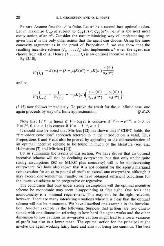
We may use Propositions 10-12 to develop a method for computing a second-best optimal incentive scheme when n = 2. Consider the case where A is finite. Recall that Proposition 6 states that, in this case, the agent will be indifferent between a* and some less costly action. This fact makes the computa- tion of an optimal incentive scheme fairly straightforward. We know from Proposition 10 that it is never optimal to get the agent to choose an inefficient action. Hence we can assume without loss of generality that CFB(al) < CFB(a2)
< ... < CFB(am) and 7T2(aI) < 7T2(a2) < ...< K 2(am). The computation of C(a,) is easy: by Remark 1 of Section 2 it is just CFB(al). To compute C(ak), k > 1, we use Propositions 6 and 11. For each action aj, j < k, find,,, I2 so that the agent is indifferent between ak and aj and the agent's expected utility is U. This means solving
G(ak) + K(ak)(7Tl(ak)Vl + 7T2(ak)V2) U,
(4.4) G(aj) + K(aj)(7gI(aj)v + 7T2(aj)V2) = Us
which yields
7T2(aJ)(U - G(ak))/lK(ak)) - 7T2(ak)(( U - G(a,))/K(aj)) V1 = 71(ak) -7l(aj)
(4.5)
7T,(aj)U - G(ak))/K(ak)) - 7T1(ak)(( U - G(a,))/K(aj)) V2 = 772(ak) -7T2(a)
We then set I, = h(v1), I2 = h(v2). Note that v1 < v2 in (4.5) so that I, < I2.

PRINCIPAL-AGENT PROBLEM 33
V2
Irl(aJ2)vl + Z2(aj2)V2 =(U-G(aj2) )/K(a12)
UI (ajl )VI + Z2 (aJI)V2 = (U-G(aJI) )/ K(al)
A
A
r(a)v
+ r2(ak)v2 =
(U-
G(ak)
) K(ak)
45~~~~~~~~~~0 VI
FIGURE 2.
Doing this for each j = 1, . . ., k - 1 yields (k - 1) different (vI,v2) (and (II' I2)) pairs, each with v1 < v2. This is illustrated in Figure 2 for the case k = 3, where the (v1, v2) pairs are at A, B. We know from Proposition 6 that one of these pairs is the solution to (2.2). In fact, the solution must occur at the (vI, v2) pair with the smallest v, (and hence, by (4.4), with the largest v2)-denote this pair by
Iv 5 '2). To see this, suppose that the agent is indifferent between ak and aj under (I v2). Consider the expression
(4.6) '7l(ak)Vl + 7T2(ak)V2 -7T,(aj)v -7T2(aj)V2
- (7T(ak) - 7T(aj))V1 + (7T2(ak) - 7T2(aj))V2
When v1 = A
= v2' this expression equals [(U - G(ak))/K(ak)]-[(U-
G(aj))/K(aj)]. Suppose now that v1 > v v2 K v2. Then (4.6) falls since 71(ak) < 7T,(aj). Hence the agent now prefers aj to ak and so ak is not implemented.
In Figure 2, the solution is at A. (The solution could not be at B since it is clear from the diagram that, at B, a12 gives the agent an expected utility greater than U, i.e. ak is not implemented at B.) Note that it is possible that the (VA, ,v
picked in this way does not lie in 91t x 9t; i.e., h(vA,) or h(vA2) may be undefined. In this case, the constraint set of (2.2) is empty and so C(ak)= x. If (vs,v2)
91t x 91, then the principal's minimum expected cost of getting the agent to pick ak is C(ak) = gl(ak)h(Al) + gl(ak)h( A2). The expected net benefits of imple- menting ak are B(ak) - C(ak). This procedure must be undergone for each ak5
34 S. J. GROSSMAN AND 0. D. HART
k = 1,.. , m. Finally, the overall optimum is determined by selecting the a which maximizes B(ak) - C(ak).
REMARK 6: In computing the cost of implementing ak, we have ignored actions which are more costly for the agent than ak. This means that the cost function which we have computed is not the true cost function C(a) but a modified cost function C(a). Clearly, C(a) < C(a) for each a since more actions can only make implementation more difficult. On the other hand, Proposition 12 tells us that maxaEA[B(a) - C(a)] < maxaeA [B(a) - C(a)]. Combining these yields maxaEA [B(a) - C(a)] = maxaEaA [B(a)- C(a)], which means that we are justified in working with C(a) instead of C(a).
Another case where computation is quite simple is when A is infinite and { CFB (a) I a E A } is an interval [c, c] of the real line. For reasons of space, we do not cover this case.
Unfortunately, the computational techniques presented above do not appear to generalize in a useful way to the case n > 2. In order to compute an optimum when n > 2, in the finite action case, it seems that we must, for each a E A, solve the convex problem in (2.2) and then, by inspection, find the a & A which maximizes B(a) - C(a). If A is infinite, one takes a finite approximation. These steps can be carried out on a computer, although the amount of computer time involved when the number of elements of A is large may be considerable.
One case where a considerable simplification can be achieved when n > 2 is where MLRC and CDFC hold. Then the solution to (2.2) has the property that (1) if A is finite, the agent is indifferent only between a*, the action the principal wants to implement, and a', where a' maximizes CFB (a) subject to CFB (a) < CFB(a*), i.e. a' is the next most costly action after a* (see the proof of Proposition 8); (2) if A is convex, then a* is the unique maximizer of G(a) +
K(a)(Evi(a)V(Il)), and [d(G(a*) + K(a*)(E7ri(a*)V(I,)))/da] = 0 is a neces- sary and sufficient condition for the agent to pick a*. In the latter case, Mirrlees [12] has shown that the first-order condition approach referred to in the introduc- _tion is valid.
One may ask also whether Propositions 10 and 12 hold in the case n > 2. The answer is no (but see Remark 7 below). Second-best optimal actions may be inefficient; i.e., there may exist lower cost actions which dominate the optimal action in the sense of first degree stochastic dominance.14 Also the addition of actions costlier than the second-best optimal action may make the principal worse off (in Example 1, the principal's expected profits increase if action a3
14LetA = {a1,a2,a3}, n = 3. Assume CFB(aI) < CFB(a2) < CFB(a3), and that 7r(aI) = (3/4, 1/8, 1/8), 7r(a2) = (1/3, 1/3, 1/3), qr(a3) = (1/2, 1/2, 0) (Assumption A3 is violated, but this is unimportant.) Then C(al) = CFB(al) since a, is the least cost action, and C(a3) = CFB(a3) since a3 can be implemented by setting II = I2, I3 = - oo. However, C(a2) > CFB(a2) and, in fact, if the agent is very risk averse, C(a2) will be so big that it is profitable for the principal to implement a3 rather than a2 (the effect of risk aversion on C(a) is discussed in Section 5). This is in spite of the fact that a3 is inefficient relative to a2.

PRINCIPAL-AGENT PROBLEM 35
becomes unavailable to the agent). Finally, as Shavell [19] has noted the agent may choose a higher cost action when there are opportunities to share risks with a principal than in the absence of these opportunities.
REMARK 7: It is interesting to note that it is possible to extend all the results of the n = 2 case to the n > 2 case when the spanning condition (SC) holds. This is because when SC holds, both the principal and the agent are essentially choosing between lotteries of the probability vectors 7T and 7A'.
In particular, let II(vl) = min1 ,n7= IJi subject to En7= I V(11)?v1;12(v2) = min{7i= I I subject to p3= 7 V(h) ? v2. Now consider the principal's minimum cost problem as: for each a*, choose v1 and v2 to minimize X(a*) 1I(vl) + (1 - X(a*))12(v2) subject to (1) G(a*) + [X(a*)vl + (1 - X(a*))v2]K(a*) > G(a) + [X(a)vl + (1 - X(a))v2]K(a) for all a E A; (2) G(a*) + [X(a*)vl + (1 -
X(a*))v2]K(a*) > U. Then the principal's problem looks exactly the same as in the n = 2 case. Note that from stochastic dominance (i.e. part (2) of the SC condition) Eni=17Tiqi < En? = 17Tqi, so "state 2" is the good state. We are grateful to Bengt Holmstrom for alerting us to the fact that all of the results for the n = 2 case hold when n > 2 and the Spanning Condition is satisfied.
5. WHAT DETERMINES HOW SERIOUS THE INCENTIVE PROBLEM IS?
In previous sections, we have studied the properties of an optimal incentive scheme. We turn now to a consideration of the factors which determine the magnitude of L, the loss to the principal from being unable to observe the agent's action.
One feels intuitively that the worse is the quality of the information about the agent's action that the principal obtains from observing any outcome, the more serious will be the incentive problem. This idea can be formalized as follows. Suppose that we start with an incentive problem in which the agent's action set is A, his utility function is U, his reservation utility is U, the probability function is 7T, and the vector of outputs is q = (ql, . . ., qn). We denote this incentive problem by (A, U, U, 7T, q). Consider the new incentive problem (A, U, U, r', q') where 7T'(a) = R7T(a) for all a E A and R is an (n x n) stochastic matrix (here 7T(a), 7T'(a) are n dimensional column vectors and the columns of R sum to one). Below we show that C'(a) > C(a) for all a E A, where unprimed variables refer to the original incentive problem and primed variables to the new incentive problem.
The transformation from 7g(a) to Rk(a) corresponds to a decrease in informa- tiveness in the sense of Blackwell (see, e.g., Blackwell and Girshick [3]).15 That is, if we think of the actions a E A as being parameters with respect to which we
'5The possibility of using Blackwell's notion of informativeness to characterize the seriousness of an incentive problem was suggested by Holmstrom [7].

36 S. J. GROSSMAN AND 0. D. HART
have a prior probability distribution, then an experimenter who makes deduc- tions about a from observing ql, ... , qn would prefer to face the function 7T than the function Rk.
PROPOSITION 13: Consider the two incentive problems (A, U, U, 7T, q), (A, U, U, 7 ',q') and assume that Assumptions A1-A3 hold for both. Suppose that 7T'(a) = R7T(a) for all a E A, where R is an (n x n) stochastic matrix. Then C'(a) > C(a) for all a E A. Furthermore, if V is strictly concave and R ?> 0,16 then CFB(a*) > minal ACFB(a) and C(a*) < xo =X C'(a*) > C(a*).
PROOF: Let (I',... , In) be the cost minimizing way of implementing a in the primed problem. Suppose that in the unprimed problem, the principal offers the agent the following random incentive scheme: for each i, if qi is the outcome, an n-sided die will be thrown where the probability of side j coming up is rjf, the (j, i)th element of R (j = 1, ... , n). If sidej then comes up, you get Ij. With this random incentive scheme, the probability of the agent getting Ij' if he chooses a particular action is the same as in the primed problem. Therefore the agent's optimal action will be a. Furthermore, the principal's expected costs are the same as in the primed problem. This shows that the principal can implement a at least as cheaply in the unprimed problem as in the primed problem by using a random incentive scheme. The final part of the proof is to note that the principal can reduce his expected cost further and continue to implement a by offering the agent the perfectly certain utility level vi = E= rj V(Ij') if the outcome is qi rather than the above lottery. That is, there is a deterministic incentive scheme which is better for the principal than the above random incentive scheme.
Q.E.D.
REMARK 8: The last part of the proof of Proposition 13 shows that it is never desirable under our assumptions for the principal to offer the agent an incentive scheme which makes his payment conditional on a particular outcome a lottery rather than a perfectly certain income.17 This result may also be found in Holmstrom [7].
Note that if g' = R7T and q'R = q, the random variable q' will have the same mean as q. In this case the following is true:
COROLLARY 1: Make the hypotheses of Proposition 13. If, in addition, q' is such that q'R = q, we have L'> L.
PROOF: Obvious since B'(a) = q'77'(a) = q'R7u(a) = q7r(a) = B(a).
16We use this notation to mean that every element of R is strictly positive. 17This result depends strongly on our Assumption Al that attitudes to income risk are indepen-
dent of action. In the absence of this assumption, random incentive schemes may be desirable.

PRINCIPAL-AGENT PROBLEM 37
In the case n = 2, the transformation X -X g' = Ru is easy to interpret. Take any two actions a, a2 E A, and consider the likelihood ratio vector ('77I(aI) /771(a2), g2(a1)/12(a2)). Assume without loss of generality that s1(a1)/s1(a2) < g2(a1)/12(a2). Then it is easy to show that
5 1 '7T(al) '7(a) 1 r '7(al) 2(al) 1 e ' L qrl(2)
' l2(2) J UX(2)
' '2(a2) ]
where [x, y] is the interval between x and y. In other words, the likelihood ratio vector becomes less variable in some sense when the stochastic transform R is applied. In fact the converse to this is also true: if (5.1) holds, then there exists a stochastic matrix R such that g' = Ru (see Blackwell and Girshick [3]). When n > 2, a simple characterization of this sort does not seem to exist, however.
One might ask whether a converse to Proposition 13 holds. That is, suppose C'(a) > C(a) for all a E A and all concave utility functions V. Does it follow that g'(a) = Rg (a) for all a E A, for some stochastic R? A converse along these lines can in fact be established when n = 2. Whether it holds for n > 2, we do not know.
Corollary 1 gives us a simple way of generating worse and worse incentive problems: repeatedly apply stochastic transforms to s. Suppose that we do this using always the same stochastic transform R, when R >> 0 and is invertible. That is, we consider a sequence of incentive problems 1,2, ..., where in the mth problem rm (a) = R' - s (a) for all a E A, and the gross profit vector q,' satisfies qmR m- I = q (this has a solution since R is invertible). We know from Corollary 1 that Lm will be increasing in m. The next proposition says that in the limit the loss from not being able to observe the agent reaches its maximal level.
DEFINITION: Let L* = maxaEA(B(a)- CFB(a)) - max{B(a')- CFB(a') I a' minimizes CFB (a) on A }.
Since C(a') = CFB(a') if a' minimizes CFB(a), L* is an upper limit on the loss to the principal from being unable to observe the agent. The next proposition shows that as the information q reveals about a gets smaller and smaller, the principal loses control over the agent, i.e., the agent chooses the least-cost action.
PROPOSITION 14: Consider the sequence of incentive problems (A, U, U, 'Tm, qm), m = 1,2,..., where 'um(a) = Rm-1(a) for all a e A, qmRm-l = q for some invertible stochastic matrix R > 0. Assume Al, A2, and ,li (a) > 0 for all i = 1, . .. , n, and a E A. Then if V is not a linear function, limmoo Lm = L*.
PROOF: It suffices to show that limmOC(a*) = x for all a* with CFB(a*) > minaEA CFB(a). Suppose not for some such a*. Let (Iml, . .. , Imn) be the cost minimizing way of implementing a* in problem m. Then ijmi(a*)Im, and
Z 17mI(a*)V(Im1) are both bounded in m. It follows from Bertsekas [2] that the (Imi) are bounded. Hence without loss of generality we may assume Imi - Ii for

38 S. J. GROSSMAN AND 0. D. HART
each i. It is easy to show that, since R is a strictly positive stochastic matrix, limm* RRm-I = R* where R* has the property that all of its columns are the same. Therefore limmO,.m(a) = R*gl(a) = X is independent of a. But this means limmOOE iqumi(a*)V(Imi) = Ei7fiV(Ii) = limmOOE i'mi(a)V(Imi) for all a E A. Hence the agent will prefer actions a with CFB(a) < CFB(a*) to a*. This contradicts the assumption that the incentive scheme implements a*. Q.E.D.
We turn now to a consideration of another factor which influences L: the agent's degree of risk aversion. Since no incentive problem arises when the agent is risk netural, but an incentive problem does arise when the agent is risk averse, one is led to ask whether L increases as the agent becomes more risk averse. One difficulty in answering this question in general is the following. The way one makes the agent more risk averse is to replace his utility function U(I,a) by H( U(I, a)) where H is a real-valued, increasing, concave function. However, if U satisfies Assumption Al, then H( U) will generally not. To get around this difficulty, we will confine our attention to the case where A is a subset of the real line, V(I) = - e-kI, G(a) = 0, and K(a) = eka, i.e., the agent's utility function is U(a,I) = -e-k(I-a), where k >0. Assume also that U= -e-ka, i.e., the agent's outside opportunity is represented by the perfectly certain income a. An increase in risk aversion can then be represented simply by an increase in k.
Note that if the agent's utility function is -e - k( -a) and U= -e - ka, then CFB(a) = a + a, which is independent of k. Hence first best profits are indepen- dent of k.
PROPOSITION 15: Consider the incentive problem (A, U, U, g, q) where A is a subset of the real line, U(a, I) = - ek( -a) a U -e - ka, and k > 0. Assume A3. Write the loss from being unable to observe the agent as L(k). Then limkOL(k)
O, limkooL(k) = L*.
PROOF: To show that limkooL(k) = L*, it suffices to show that limkOoC(a*, k) = x for all a* with CFB(a*) > minaEA CFB(a). Suppose not for some such a*, and let CFB(a) < CFB(a*). Then if (II, . .. , In) implements a*, we must have
-(E (a*)e - kI)eka* > ( E? (a)e-kI)eka
(II ... , In of course depend on k). Therefore,
(5.2) ek(a*-a) <3gi(a)e-kI ,3T(a*)ek-
i i
Now let k - x. The LHS of (5.2) - x. Therefore so must the RHS. We may assume w.l.o.g., however, that I, = miniIi. Then
is i (a)e kth denomi (a)e k(C t io,)
Zjigi(a*)e- kl E i7i(a*)e k(I I-I,)'
which is bounded since the denominator > gl(a*). Contradiction.

PRINCIPAL-AGENT PROBLEM 39
We show now that limk,OL(k) = 0. Let Ii = qi- F. Then the agent maximizes
(5.3) E(-ek( a))=-E(1-k(I-a)+ k (I- a)2+ )
I- + k( Y. qri(a)qi -F - a) k2- E(I -a)2 +*--
It follows that the agent maximizes
(Z,gj(a)q - F -a) - E(I -a ...
which means that in the limit k -*0 the agent maximizes B(a) - CFB(a), i.e. chooses a first-best action. Furthermore, setting (5.3) equal to -e-k= 1 + ka + * , we see that in the limit k - 0,
max (Z3ri(a)qi-a)-F=a,
so that the principal's expected profit equals F = maxaEA (A,i qi -a) - a = maxa E A (B (a) - CFB (a)) = first-best profit. Q.E.D.
Proposition 15 tells us about the behavior of L(k) for extreme values of k. It would be interesting to know whether L(k) is increasing in k. We do not know the answer to that question except for the case n = 2, A finite.
PROPOSITION 16: Make the same hypotheses as in Proposition 14. Assume in addition that n = 2 and A is finite. Then L(k) is increasing in k.
PROOF: See Appendix.
REMARK 9: Propositions 15 and 16 tell us how the principal's welfare varies with k. It is also interesting to ask how the shape of the optimal incentive scheme depends on k. Unfortunately, even in the case n = 2, very little can be said. In this case, the incentive scheme is characterized by the agent's share s. It is not difficult to construct examples showing that an increase in the agent's risk aversion may increase the optimal value of s, or may decrease it.
We conclude this section by considering how L depends on the agent's incremental costs. Consider the case of additive separability, i.e., K(a)
constant. Suppose that we write the agent's utility function as Uj(a, I) = Gj(a) + V(I), where Gj(a) = a + XF(a), X > 0. (Without loss of generality, we take K = 1.) Then, when X is small, one feels that L will be small since the agent does not require much of a reward to work hard. The fact that limx,OL(X) = 0 has in fact been established by Shavell [20]. We prove a somewhat stronger result.
PROPOSITION 17: Consider the incentive problem (A, U,, U, g, q), where U,(a, I) = a + XF(a) + V(I) for all a e A, X > 0. Assume that A1-A3 hold for this

40 S. J. GROSSMAN AND 0. D. HART
problem. Assume also that (1) A is an interval of the real line; (2) B(a) and F(a) are twice differentiable in the interior of A; (3) V is twice differentiable on 4 and V' > 0; (4) There is a unique maximizer a* of B(a) lying in the interior of A and B"(a*) < 0. Then limX>0(L(X)/X) = 0.
PROOF: Consider the incentive problem with X = 1. Then there are a's arbi- trarily close to a* for which C(a) is finite. For let the principal set vi = rq, - k where k is chosen so that vi E Qt for all i. Then the agent will maximize
Zri (a) U(a, I), i.e. T(a)q, + F(a)/r. By letting r - x, we can get the agent to choose an action arbitrarily close to a*. For such an action, C(a) will be finite.
Consider now an a arbitrarily close to a*. Let (v,, . . . , v") be the cost minimizing way of implementing a when X = 1. Then it is clear from (2.2) that
(Xv, + 1B, . .. , Xvn + 3) will implement a for A # 1, where
X(ZTj(a)vj + F(a)) + ae + /3=U.
It follows that
L(X) a - 1 h( )qa-h (U- a-XF(a))
- (E 7r(a)qj - E7T(a)h(Xvi + 13)),
where a maximizes E i(a)qi - h(U - a - XF(a)), i.e. a is the first-best action in problem X.
Therefore,
X < [ A( Xi(a*) qj-h (U-a-XF(a*))
- (E'ui(a)q, - '7T,(a)h(Xvj + /e))
[ { ar()q, - h(U-a -XF(a))
- Ev7i(a*)qi + h(U-a - XF(a*)) }
Now a- a* as X--> 0. Furthermore, by differentiating the first-order conditions
(dl a)(2Mri(a) - h(U-a - XF()) =, one can show that dl/dX exists at X = 0. It follows from the mean-value theorem and the fact that B'(a*) = 0 that the second square bracket -> as X -0. To see that the first square bracket - 0, note that, since a is arbitrary, we can make a converge to a* as fast as we like. Therefore we need only show that
{X; AA lim E 7v r (a)h(v +\1 ERA h(T a -t_ X F(a*) = n.

PRINCIPAL-AGENT PROBLEM 41
But
r7T(a)[h(vi + hv ) )-h(U-a -XF(a*))]
- 37Xi(a)[ h (Xv + U-a - - X(a)v.-F(a))
- h ( U-at- XF(a*))|
- 2 7T1(a)[ h (U-a) + h'(U-a))(Xv -X 3 i(a)v, -XF(a))
+ h.. -h(U-a) + h'(U-a)(XF(a*)) +
- h'( U + a)(- XF(a) + XF(a*)) + *
from which (5.4) follows. Q.E.D.
The proof of Proposition 17 is based on an envelope argument. It appears that a similar result can be established for the more general case where U is not additively separable, but Assumption Al holds. Since the proof is more compli- cated, however, we will not pursue this result here. The assumption that a* lies in the interior of A may seem quite strong. Note, however, that if a* is a boundary point and B'(a*) #, 0, then the second-best optimal action equals a* for small enough X. It is straightforward to apply the proof of Proposition 17 to show that limx,0(L(X)/X) = 0 in this case too.
Since the marginal product of labor of the agent-that is, the increase in expected profit resulting from an extra pound of expenditure by the agent-is proportional to 1 /X, Proposition 17 can be interpreted as saying that the welfare loss L is of a smaller order of magnitude than the reciprocal of the agent's marginal product of labor.
6. EXTENSIONS
We have assumed throughout the paper that the principal is risk-neutral and that the agent's attitudes to risk over income lotteries are independent of action -Assumption Al. We now briefly consider what happens if we relax these assumptions.
As we have noted in Section 2, Remark 3, our method of analysis generalizes without any difficulty to the case where the principal is risk-averse. Specific results change, however, The main difference is that now, even in the first-best situation, the principal will not bear all the risk. One implication of this is that even if there is no disutility of action for the agent, i.e. a does not enter the agent's utility function, the first-best will not generally be reached. The reason is that there may be a conflict between the principal and agent over what income lottery should be selected (for a study of this conflict, see Ross [17] and Wilson [23]).
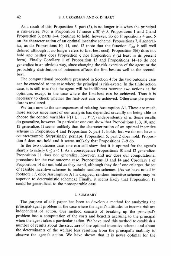
42 S. J. GROSSMAN AND 0. D. HART
As a result of this, Proposition 3, part (5), is no longer true when the principal is risk-averse. Nor is Proposition 17 since L(0) , 0. Propositions 1 and 2 and Proposition 3, parts 1-4, continue to hold, however. So do Propositions 4 and 5 on the characterization of an optimal incentive scheme. Propositions 7, 8 general- ize, as do Propositions 10, 11, and 12 (note that the function CFB is still well defined although it no longer refers to first-best cost). Proposition 3(6) does not hold and neither does Proposition 6 nor Proposition 9 (at least in its present form). Finally Corollary 1 of Proposition 13 and Propositions 14-16 do not generalize in an obvious way, since changing the risk aversion of the agent or the probability distribution of outcomes affects the first-best as well as the second- best.
The computational procedure presented in Section 4 for the two outcome case can be extended to the case where the principal is risk-averse. In the finite action case, it is still true that the agent will be indifferent between two actions at the optimum, except in the case where the first-best can be achieved. Thus it is necessary to check whether the first-best can be achieved. Otherwise the proce- dure is unaltered.
We turn now to the consequences of relaxing Assumption Al. These are much more serious since most of our analysis has depended crucially on being able to choose the control variables V(Ij), . . . , V(I,) independently of a. Some results do generalize, however. In particular one can show that Propositions 1, 3, 10, and 12 generalize. It seems unlikely that the characterization of an optimal incentive scheme in Proposition 4 and Proposition 5, part 1, holds, but we do not have a counterexample. Surprisingly, perhaps, Proposition 5, part 2 does hold. Proposi- tion 6 does not hold and it seems unlikely that Propositions 7-9 do.
In the two outcome case, one can still show that it is optimal for the agent's share s to satisfy 0 < s < 1. As a consequence Propositions 10 and 12 generalize. Proposition 11 does not generalize, however, and nor does our computational procedure for the two outcome case. Propositions 13 and 14 and Corollary 1 of Proposition 14 do not hold as they stand, although they do if one enlarges the set of feasible incentive schemes to include random schemes. (As we have noted in footnote 17, once Assumption Al is dropped, random incentive schemes may be superior to deterministic schemes.) Finally, it seems likely that Proposition 17 could be generalized to the nonseparable case.
7. SUMMARY
The purpose of this paper has been to develop a method for analyzing the principal-agent problem in the case where the agent's attitudes to income risk are independent of action. Our method consists of breaking up the principal's problem into a computation of the costs and benefits accruing to the principal when the agent takes a particular action. We have used this method to establish a number of results about the structure of the optimal incentive scheme and about the determinants of the welfare loss resulting from the principal's inability to observe the agent's action. We have shown that it is never optimal for the

PRINCIPAL-AGENT PROBLEM 43
incentive scheme to be such that the principal's and agent's payoff are negatively related over the whole outcome range, although such a relationship may be optimal over part of the range. We have found sufficient conditions for the incentive scheme to be monotonic, progressive, and regressive. We have shown that a decrease in the quality of the principal's information in the sense of Blackwell increases welfare loss. When there are only two outcomes, welfare loss also increases when the agent becomes more risk averse. Finally, we have discussed how our techniques can be used to compute optimal incentive schemes in particular cases.
While we have talked throughout about "the" principal-agent problem, we have in fact been considering the simplest of a number of such problems. More complicated principal-agent problems arise when not only is the principal unable to monitor the agent, but also the agent possesses information about his environ- ment, i.e. about A, gr, or U(a, I), which the principal does not. Such problems possess a number of features of the preference revelation problems studied in the recent incentive compatibility literature; see, for example, the Review of Economic Studies Symposium [16]. A start has been made in the analysis of such problems by Harris and Raviv [6], Holmstrom [7], and Mirrlees [12]. It will be interesting to see whether the techniques presented here will also be useful in the solution of these more complicated principal-agent problems.
University of Chicago and
London School of Economics
Manuscript received September, 1980; revisions received September, 1981.
APPENDIX
PROOF OF PROPOSITION 16: It suffices to show that C(a, k) is increasing locally in k for each a E A whenever C(a, k) is finite. Let k = Xk A > 1. Assume that (II, I2) iS the cost minimizing way of implementing a, given k. Then, by the results of Section 4, e.g. equation (4.4),
1TIWI + 7T2W2 = ek(Qa +a)
(A1)
ST'IWI + 7T2W2 = et?
where w,
= e-k)1, w2 =ek12, I = 7TI(a), 7T2 = 7T2(a), 7iT = VTI(a'), 7T = VT2(a) a' E A, a' < a. Fur-
thermore we can pick a' so that a' is independent of k for X close to 1. Equations (Al) determine w1 and w2 for each value of k. The cost of implementing a, C(a, k), is
then given by
(A2) C(a, k)= 7rII I+ 7T2'2 -I (7r1logWI + rT2logW2). k
Differentiating (A2) with respect to X we get
aC(a,Xk) 1 1 VT dw1 V72 dW2 (A3) ax I = T1goWg + 7T21ogW2- ------1 (A3) x X= k w1 dA w2 dA

44 S. J. GROSSMAN AND 0. D. HART
Set x = e k(a+a), y = e-k(a' +a) in (Al). Then e-k(a+a) = X, e-k a'+a) =y'7 Hence
dw1 dw2 dX +7T2 dW2 =xlogx, dX dX
(A4) dw I dw2
dX +72 dX =Ylogy,
where derivatives are evaluated at X= 1. Solving (Al), (A4) yields
7X - 7T2Y 7T2X -7T2Y
7172- 7172 7T2 -72
dw1 _ X logx-7T2Y log y
dX 7g2-7T2
It follows that logw1 > (l/w1)(dwI/dA). For
dw1 7T2X-7T2 y 7T2'X- 7T2 y / 7T'X log x- 7T2 y 10g y (A5) w1log,w1- d , log2, - dX T-7T2 7T - 7T2 7T - 7T2
7T2-7T2 [(ax - y)log ax -ax logx -y log y]
where a = 72, , = 7T2. However, the RHS of (A5) > 0 by Lemma 3 below. The same argument shows that logw2 > (l/w2)(dw2/dA). It follows from (A3) that (aC/lX) > 0, i.e., C is increasing locally in k.
LEMMA 3: Assume a, 3, x, y > 0. Then if a > 8 and ax > /y, ax log x-/3y log < (ax-/3y) log((ax - /y)/(a - /)). On the other hand, if a < 8 and ax < fy, ax log x - fy log y > (ax - fy) log((ax - fy)/(a - /)).
PROOF: Since z logz is a convex function,
(y logy) + (a /)( - y log
a - ) > x logx.
This proves the first part. The second part follows similarly. Q.E.D.
REFERENCES
[1] ARROW, K. J.: "Insurance, Risk and Resource Allocation," Essays in the Theory of Risk Bearing. Chicago: Markham, 1971.
[2] BERTSEKAS, D.: "Necessary and Sufficient Conditions for Existence of an Optimal Portfolio," Journal of Economic Theory, 8(1974), 235-247.
[3] BLACKWELL, D., AND M. A. GIRSHICK: Theory of Games and Statistical Decisions. New York: John Wiley and Sons, Inc., 1954.
[4] BORCH, K.: The Economics of Uncertainty. Princeton: Princeton University Press, 1968. [5] HARDY, G. H., J. E. LITTLEWOOD, AND G. POLYA: Inequalities. Cambridge: Cambridge Univer-
sity Press, 1952. [6] HARRIS, M., AND A. RAVIV: "Optimal Incentive Contracts with Imperfect Information," Journal
of Economic Theory, 20(1979), 231-259. [7] HOLMSTROM, B.: "Moral Hazard and Observability," Bell Journal of Economics, 10(1979), 74-91. [8] KEENEY, R.: "Risk Independence and Multiattributed Utility Functions," Econometrica,
41(1973), 27-34. [9] MILGROM, P. R.: "Good News and Bad News: Representation Theorems and Applications,"
Discussion Paper No. 407, Northwestern University, Illinois, Mimeo, 1979.

PRINCIPAL-AGENT PROBLEM 45
[10] MIRRLEES, J. A.: "The Theory of Moral Hazard and Unobservable Behavior-Part I," Nuffield College, Oxford, Mimeo, 1975.
[11] : "The Optimal Structure of Incentives and Authority Within an Organization," Bell Journal of Economics, 7(1976), 105-131.
[12] : "The Implications of Moral Hazard for Optimal Insurance," Seminar given at Confer- ence held in honour of Karl Borch, Bergen, Norway, Mimeo, 1979.
[13] PAULY, M.: "The Economics of Moral Hazard: Comment," American Economic Review, 58(1968), 531-536.
[14] POLLAK, R.: "The Risk Independence Axiom," Econometrica, 41(1973), 35-39. [15] RADNER, R.: "Monitoring Cooperative Agreements in a Repeated Principal-Agent Relation-
ship," Mimeo, Bell Laboratories, 1980. [16] Review of Economic Studies Symposium on Incentive Compatibility, April, 1979. [17] Ross, S.: "The Economic Theory of Agency: The Principal's Problem," American Economic
Review, 63(1973), 134-139. [18] RUBINSTEIN, A. AND M. YAARI: Seminar given at Conference held in honour of Karl Borch,
Bergen, Norway, 1979. [19] SHAVELL, S.: "On Moral Hazard and Insurance," Quarterly Journal of Economics, 93(1979),
541-562. [20] : "Risk Sharing and Incentives in the Principal and Agent Relationship," Bell Journal of
Economics, 10(1979), 55-73. [21] SPENCE, M., AND R. ZECKHAUSER: "Insurance, Information, and Individual Action," American
Economic Review, 61(1971), 380-387. [22] STIGLITZ, J. E.: "Incentives and Risk Sharing in Sharecropping," Review of Economic Studies,
61(1974), 219-256. [23] WILSON, R.: "The Theory of Syndicates," Econometrica, 36(1968), 119-132. [24] ZECKHAUSER, R.: "Medical Insurance: A Case Study of the Trade-Off Between Risk Spreading
and Appropriate Incentives," Journal of Economic Theory, 2(1970), 10-26.