The Principal-Agent Alignment Problem in Artificial ...
166
The Principal-Agent Alignment Problem in Artificial Intelligence Dylan Hadfield-Menell Electrical Engineering and Computer Sciences University of California, Berkeley Technical Report No. UCB/EECS-2021-207 http://www2.eecs.berkeley.edu/Pubs/TechRpts/2021/EECS-2021-207.html August 26, 2021
Transcript of The Principal-Agent Alignment Problem in Artificial ...

The Principal-Agent Alignment Problem in Artificial
Intelligence
Dylan Hadfield-Menell
Electrical Engineering and Computer SciencesUniversity of California, Berkeley
Technical Report No. UCB/EECS-2021-207
http://www2.eecs.berkeley.edu/Pubs/TechRpts/2021/EECS-2021-207.html
August 26, 2021

Copyright © 2021, by the author(s).All rights reserved.
Permission to make digital or hard copies of all or part of this work forpersonal or classroom use is granted without fee provided that copies arenot made or distributed for profit or commercial advantage and that copiesbear this notice and the full citation on the first page. To copy otherwise, torepublish, to post on servers or to redistribute to lists, requires prior specificpermission.
Acknowledgement
I am deeply grateful to my advisors for their guidance, support, andpatience throughout this process. It has been an honor to be your studentand I look forward to the opportunity to collaborate again in the future.Thank you for helping shape me into the researcher that I am today. Thank you to my family for their support and flexibility throughout graduateschool. I know it was difficult at times, but I could not have done it withoutyour support. Last, and most importantly, thank you to Veronica, for yourcommitment to my dreams and for the work to help me get there.

The Principal–Agent Alignment Problem in Artificial Intelligence
by
Dylan Jasper Hadfield-Menell
A dissertation submitted in partial satisfaction of the
requirements for the degree of
Doctor of Philosophy
in
Computer Science
in the
Graduate Division
of the
University of California, Berkeley
Committee in charge:
Professor Stuart J. Russell, Co-chairProfessor Anca D. Dragan, Co-chair
Professor Pieter AbbeelProfessor Ken Goldberg
Summer 2021

The Principal–Agent Alignment Problem in Artificial Intelligence
Copyright 2021by
Dylan Jasper Hadfield-Menell

1
Abstract
The Principal–Agent Alignment Problem in Artificial Intelligence
by
Dylan Jasper Hadfield-Menell
Doctor of Philosophy in Computer Science
University of California, Berkeley
Professor Stuart J. Russell, Co-chair
Professor Anca D. Dragan, Co-chair
The field of artificial intelligence has seen serious progress in recent years, and has also causedserious concerns that range from the immediate harms caused by systems that replicateharmful biases to the more distant worry that effective goal-directed systems may, at a certainlevel of performance, be able to subvert meaningful control efforts. In this dissertation, Iargue the following thesis:
1. The use of incomplete or incorrect incentives to specify the target behavior for anautonomous system creates a value alignment problem between the principal(s), onwhose behalf a system acts, and the system itself;
2. This value alignment problem can be approached in theory and practice through thedevelopment of systems that are responsive to uncertainty about the principal’s true,unobserved, intended goal; and
3. Value alignment problems can be modelled as a class of cooperative assistance games,which are computationally similar to the class of partially-observed Markov decisionprocesses. This model captures the principal’s capacity to behave strategically in coor-dination with the autonomous system. It leads to distinct solutions to alignment prob-lems, compared with more traditional approaches to preference learning like inversereinforcement learning, and demonstrates the need for strategically robust alignmentsolutions.
Chapter 2 goes over background knowledge needed for the work. Chapter 3 argues the firstpart of the thesis. First, in Section 3.1 we consider an order-following problem between arobot and a human. We show that improving on the human player’s performance requires
2
that the robot deviate from the human’s orders. However, if the robot has an incompletepreference model (i.e., it fails to model properties of the world that the person does careabout), then there is persistent misalignment in the sense that the robot takes suboptimalactions with positive probability indefinitely. Then, in Section 3.2, we consider the problemof optimizing an incomplete proxy metric and show that his phenomenon is a consequenceof incompleteness and shared resources. That is, we provide general conditions under whichoptimizing any fixed incomplete representation of preferences will lead to arbitrarily largelosses of utility for the human player. We identify dynamic incentive protocols and impactminimization as theoretical solutions to this problem.
Next, Chapter 4 deals with the second part of the thesis. We first show, in Section 4.1,that uncertainty about utility evaluations creates incentives to get supervision from thehuman player. Then, in Section 4.2 and Section 4.3, we demonstrate how to use uncertaintyabout utility evaluations to implement reward learning approaches that penalize negativeside-effects and support dynamic incentive protocols. Specifically, we show how to applyBayesian inference to learn a distribution over potential true utility functions, given theobservation of a proxy in a specific development context.
Chapter 5 deals with the third part of the thesis. We introduce cooperative inverse rein-forcement learning (Cirl), which formalizes the base case of assistance games. Cirlmodelsdyadic value alignment between a human principal H and a robot assistant R. This game-theoretic framework models H’s incentive to be pedagogic. We show that pedagogical so-lutions to value alignment can be substantially more efficient than methods based on, e.g.,imitation learning. Additionally, we provide theoretical results that support a family of effi-cient algorithms for Cirl that adapt standard approaches for solving PoMdps to computepedagogical equilibria.
Finally, Chapter 6 considers the final component of the thesis, the need for robust solutionsthat can handle strategy variation on the part of H. We introduce a setting where R assistsH in solving a multi-armed bandit. As in Section 3.1, H’s actions tell R which of the kdifferent arms to pull. However, this introduces the complication that H does not knowwhich arm is optimal a priori. We show that this setting admits efficient strategies where Htreats their actions as purely communicative. These communication solutions can achieveoptimal learning performance, but perform arbitrarily poorly if the encoding strategy usedby H is misaligned with R’s decoding strategy.
We conclude with a discussion of related work in Chapter 7 and proposals for future workin Chapter 8.

i
Contents
Contents i
1 Introduction 11.1 The alignment problem in artificial intelligence . . . . . . . . . . . . . . . . . 11.2 Incentives as a programming language for behavior . . . . . . . . . . . . . . 21.3 Incompleteness and overoptimization . . . . . . . . . . . . . . . . . . . . . . 61.4 Building systems that respond to uncertainty about goals . . . . . . . . . . . 71.5 The promise and perils of pedagogy . . . . . . . . . . . . . . . . . . . . . . . 81.6 Overview . . . . . . . . . . . . . . . . . . . . . . . . . . . . . . . . . . . . . . 9
2 Preliminaries 122.1 Markov Decision Process . . . . . . . . . . . . . . . . . . . . . . . . . . . . . 122.2 Partially-Observed Markov Decision Process . . . . . . . . . . . . . . . . . . 152.3 Inverse Reinforcement Learning . . . . . . . . . . . . . . . . . . . . . . . . . 18
3 Misalignment 223.1 A Supervision POMDP . . . . . . . . . . . . . . . . . . . . . . . . . . . . . . 233.2 Overoptimization . . . . . . . . . . . . . . . . . . . . . . . . . . . . . . . . . 313.3 Mitigating Overoptimization: Conservative Optimization and Dynamic In-
centive Protocols . . . . . . . . . . . . . . . . . . . . . . . . . . . . . . . . . 41
4 Uncertainty 484.1 Incentives for Oversight . . . . . . . . . . . . . . . . . . . . . . . . . . . . . 494.2 Inverse Reward Design . . . . . . . . . . . . . . . . . . . . . . . . . . . . . . 544.3 Implementing a dynamic incentive protocol . . . . . . . . . . . . . . . . . . . 67
5 Pedagogy 795.1 Pedagogic principals are easier to assist . . . . . . . . . . . . . . . . . . . . . 815.2 Cooperative Inverse Reinforcement Learning . . . . . . . . . . . . . . . . . . 87
6 Robust Alignment 1096.1 Exploring strategy robustness in ChefWorld . . . . . . . . . . . . . . . . . . 1106.2 Assisting a Learning H . . . . . . . . . . . . . . . . . . . . . . . . . . . . . . 111

ii
6.3 Reward Communication Equilibria in Assistive-MABs . . . . . . . . . . . . . 121
7 Related Work 1297.1 The Economics of Principal–Agent Relationships and Incomplete Contracting 1297.2 Impact Minimization . . . . . . . . . . . . . . . . . . . . . . . . . . . . . . . 1337.3 Inverse Reinforcement Learning . . . . . . . . . . . . . . . . . . . . . . . . . 1347.4 Reward Learning . . . . . . . . . . . . . . . . . . . . . . . . . . . . . . . . . 1357.5 Optimal Reward Design . . . . . . . . . . . . . . . . . . . . . . . . . . . . . 1367.6 Pragmatics . . . . . . . . . . . . . . . . . . . . . . . . . . . . . . . . . . . . 1367.7 Corrigible Systems . . . . . . . . . . . . . . . . . . . . . . . . . . . . . . . . 1377.8 Intent Inference For Assistance . . . . . . . . . . . . . . . . . . . . . . . . . 1377.9 Cooperative Agents . . . . . . . . . . . . . . . . . . . . . . . . . . . . . . . . 1387.10 Optimal Teaching . . . . . . . . . . . . . . . . . . . . . . . . . . . . . . . . . 1397.11 Algorithms for Planning with Partial Observability . . . . . . . . . . . . . . 139
8 Directions for Future Work 141
Bibliography 145

iii
Acknowledgments
I am deeply grateful to my advisors for their guidance, support, and patience throughoutthis process. It has been an honor to be your student and I look forward to the opportunityto collaborate again in the future. Thank you for helping shape me into the researcher thatI am today.
To Prof. Anca Dragan, thank you for the joy you brought to research meetings, forteaching me to be experimentally rigorous, and for sharing your insight into the nature ofpractical, algorithmic, human-robot interaction. To Prof. Stuart Russell, thank you forteaching me to do careful research, for always taking the time to discuss the bigger picturebehind a research project, and for your guidance on how to write clearly and persuasively.To Prof. Pieter Abbeel, thank you for the opportunity to develop my skills as a mentor, foryour support in that process, and for pushing me to go beyond my research comfort zone.
I would also like to thank Prof. Ken Goldberg for serving on my committee and forinviting me to collaborate with him and his students. I am also indebted to the students(undergraduate and graduate) that I have had the opportunity to work with. Thank youfor making research fun and helping me to take breaks when I needed to. Thank you to thestaff at the Center for Human-Compatible AI and the Berkeley AI Research Lab for theirassistance managing the details of research.
Thank you to my family for their support and flexibility throughout graduate school. Iknow it was difficult at times, but I could not have done it without your support. Last, andmost importantly, thank you to Veronica, for your commitment to my dreams and for thework to help me get there.
This dissertation collects and combines results developed in collaboration with, in ad-dition to my advisors, Lawrence Chan, Jaime K. Fisac, Gillian K. Hadfield, Dhruv Ma-lik, Smitha Milli, Malayandi Palaniappan, Ellis Ratner, Siddhartha Srinivasa, and SimonZhuang. I am grateful to each and every one for their contributions. Portions of this texthave been adapted from Chan et al. [31], Malik et al. [104], Hadfield-Menell and Hadfield [67],Milli et al. [109], Ratner, Hadfield-Menell, and Dragan [124], Zhuang and Hadfield-Menell[180], and Hadfield-Menell et al. [70, 73]. The terminology for pedagogic equilibrium wasinitially introduced in Fisac et al. [46]. This work was supported by a Berkeley Fellowship,National Science Foundation Graduate Research Fellowship Grant No. 1106400, the Centerfor Human-Compatible AI, FLI, OpenPhil, OpenAI, ONR, NRI, AFOSR, and DARPA.

1
Chapter 1
Introduction
1.1 The alignment problem in artificial intelligence
The field of artificial intelligence has made remarkable progress in the ability to programcomputers with goal-driven behaviors in response to visual, linguistic, and other perceptualinput [179]. This includes more abstract achievements such as superhuman performance inzero-sum games [144, 110] and deployed commercial products such as data-driven recom-mendation systems that direct and monetize attention online [50, 174]. At the same time,the deployment of these systems has been accompanied by several high-profile failures andincreasingly vocal concerns.
When we look at these examples, we can identify two types of failures. The first is anold story in the development of new technology: the system designers over-promised andthe algorithm did not perform as intended. For example, consider the instances of fatalcar accidents caused by Tesla’s autopilot system [21]. In principle, better computer visiontechniques, in the sense of more effective optimization of empirical and ‘true’ risk, can reducethe occurrence of these types of failures.
In the other cases, however, the failure stems from the system effectively optimizing forits stated objective. Consider the engagement optimization techniques used in recommen-dation systems [158]. These systems have come under serious scrutiny for their propensityto promote polarizing [16], addictive [76, 10], or extremist [79] content. It is clear that theseharms are not a result of a machine learning failure — instead they are a good exampleof the system optimizing a narrowly defined objective effectively.1 The propensity of opti-mized behavior to produce surprising, unintended results, has been observed in economicinteractions [85] and autonomous systems [90].
1It is important to note that the problems observed in online platforms go beyond algorithmic chal-lenges. Even with the ability to define the goal of ‘good’ engagement, there are regulatory challenges ingetting companies to adopt those definitions and ethical questions to consider about who should providesuch definitions. For this work, the core point is that we do not yet have clear techniques for how to providethese definitions.

CHAPTER 1. INTRODUCTION 2
In these situations, the goal specified by the system designer is faulty. Thus, improve-ments in the capabilities of AI systems, measured against their ability to optimize a giventask, will not reduce the risk of these harms. In fact, we can expect that progress alongthe current trajectory of AI technology will increase the costs of misspecification for tworeasons: First, more capable systems are more likely to be deployed in consequential settingswhere they can cause harm. Second, they will be more effective at exploiting gaps betweena specified objective and the intended goal.
In this dissertation, I will argue that this type of failure is a direct consequence of thedesign pattern that has become dominant in the field of artificial intelligence. We will referto this class of failures where the system malfunctions because it optimizes its objectivetoo effectively as alignment failures. While misspecification is a challenge in any engineeringapplication, I will argue that the nature of incentives and optimal behavior make this problemespecially challenging and consequential in artificial intelligence. My thesis consists of threecomponents:
1. The use of incomplete or incorrect incentives to specify the target behavior for anautonomous system creates a value alignment problem between the principal(s), onwhose behalf a system acts, and the system itself;
2. This value alignment problem can be approached in theory and practice through thedevelopment of systems that are responsive to uncertainty about the principal’s true,unobserved, intended goal; and
3. Value alignment problems can be modelled as a class of cooperative assistance games,which are computationally similar to the class of partially-observed Markov decisionprocesses. This model captures the principal’s capacity to behave strategically in coor-dination with the autonomous system. It leads to distinct solutions to alignment prob-lems, compared with more traditional approaches to preference learning like inversereinforcement learning, and demonstrates the need for strategically robust alignmentsolutions.
1.2 Incentives as a programming language for
behavior
Before we discuss the problems caused by the use of incentives in the design of AI systems,it is useful to consider, first, why they have become the dominant paradigm in the field.One of the core challenges in the design of ‘intelligent’ autonomous systems is the need tobalance three competing goals:
1. The program class used to represent the behaviors needs to be flexible enough that itcan represent the desired behavior.

CHAPTER 1. INTRODUCTION 3
Figure 1.1: This dissertation formalizes the principal–agent alignment problem in artificialintelligence. Left: Most modern approaches to the design of autonomous systems rely onincentives to specify desired behavior. When these incentives are incomplete or incorrect,this creates a misalignment between the robot’s objective, depicted as a proxy metric
∼r, and
the principal’s intended goal, depicted as U . We argue in Chapter 3 that this misalignmentcan easily lead the system to perform poorly, perhaps catastrophically so. Right: A de-piction of cooperative inverse reinforcement learning (Cirl). Cirl, which we formalize inChapter 5, models value alignment as a cooperative assistance game where the true objec-tive is unobserved by the robot R and is revealed through the principal’s actions depictedas ~aH. Crucially, Cirl models the principal’s incentive to behave pedagogically (i.e., teachR) and leads to distinct solutions to alignment problems, compared with more traditionalapproaches to preference learning such as inverse reinforcement learning.
2. The program class used needs to be simple enough that a real person can, directly orindirectly, specify an acceptable behavior out of the large set of alternatives.
3. The program representation needs to be such that it can be executed on high-dimensionalperceptual input under time, energy, and other computational constraints.
While general-purpose programming languages are flexible enough that they could, intheory, represent a wide variety of interesting behaviors, it is simply too difficult for ahuman to directly encode a policy that, e.g., reliably navigates a mobile robot through acluttered environment. Similar statements apply to language processing, high-dimensionalmotor control, and other subareas of artificial intelligence. One way to understand theissue is that the vast majority of programs exhibit highly uninteresting behavior when runon realistic perceptual input. Getting a system to do anything that resembles coherentbehavior at all is a huge challenge.

CHAPTER 1. INTRODUCTION 4
In response to these challenges, the field of artificial intelligence developed a design pat-tern that lowers the burden on the designer. First, the field undertook a serious computa-tional study of rational decision making and utility maximization. This allowed researchersto shift from the problem of specifying behaviors to specifying goals and allowing a general-purpose optimization algorithm to identify the correct actions to take. In effect, this preventssystem designers from specifying behaviors that are useless: if the optimization algorithmruns correctly, then, at a minimum, any behavior executed will accomplish some objective.
The second major development was the adoption of statistical methods and probabilisticinference. It is not enough to program goal-achieving behaviors in an abstract model ofthe world. Mismatches between the abstract model and reality inevitably lead to undesiredbehavior. This is exemplified in robotics applications, where, e.g., uncertainty about thedynamics of the world and the impact of different controls on the world state make it hardto directly specify an accurate model. Probabilistic inference provided AI researchers withthe ability to adapt models to observed data. Although much work remains to be done,these two developments give the designers of AI systems a plausible method to implementprograms that execute coherent behaviors in the real world. The problem of ‘programming’an AI system is then reduced to the problem of specifying the correct goal as, e.g., anempirical loss function for supervised learning or a reward function for policy optimization.
As a result, the field has invested heavily in the development of tools that functionanalogously to compilers. We have developed representation languages for incentives that,although not directly executable, can be converted into executable programs in a general-purpose manner. Just as a compiler takes an abstract representation of a program (e.g.,in C code) and produces an executable program (e.g., machine code), a supervised learningalgorithm takes an abstract representation of behavior (e.g., a dataset of images labelled cator dog) and produces an executable representation of that behavior (e.g., a set of neuralnetwork weights for an image classification network).
At this point, we have built existence proofs of effective compilers. However, our researchproblems are analogous to benchmark code snippets for compiler research. As AI systemsleave the lab, we will need to develop new compilers that can handle and support effectivedevelopment environments. What properties make for a good behavior compiler? How dowe build robust development practices for these software systems? How do we make surethey provide value for individuals and society?
It is clear that the specification of a ‘good’ compiler in this context includes much morethan its ability to accomplish a specified goal. Let us return to the content recommendationexample. The system’s goal is to find ‘good’ content, in this case defined as content peoplewill interact with. While this is reasonable in many cases, it has become clear that a lot ofthe most engaging content on the internet has undesirable properties. In this sense, we caninterpret the system’s misbehavior as a result of optimizing its objective ‘too much.’
We will use the term overoptimization to refer to situations like this, where optimizedbehavior produces unwanted outcomes that score well according to the specified objectivebut not the true objective. This has long been observed as a property of incentive-drivenbehavior in humans. Kerr [85] discusses “the folly of rewarding A, while hoping for B” in a

CHAPTER 1. INTRODUCTION 5
variety of social settings. One salient example is that of organized cheating in universities,where students are rewarded for good grades while society hopes that they will gain trueknowledge. Goodhart [59] and Campbell [26] observed similar issues with respect to publicpolicy where market actors demonstrate the ability to game policy metrics and subvertintended policy goals. Strathern [157] articulated this phenomenon well in the context ofteaching quality audits in British universities: “once a measure becomes a target, it ceasesto be a good measure.”2
In the study of artificial intelligence, overoptimization has received relatively little study,with one large exception: the classic machine learning problem of overfitting. Overfittingoccurs when, e.g., a supervised learning system selects a classifier that reflects the noise inthe data instead of the underlying concept the designers care about. This leads to highperformance on the training data (i.e., effective optimization of the specified goal) but poorperformance on new data. From an alignment perspective, we can understand this as acapable system that learns to exploit the gap between the goal we are able to specify (em-pirical risk) and the goal we actually care about (true risk on new data). Results that provethe consistency of learning methods can be understood as identifying a family of finite-sizeincentives (i.e., labelled datasets) that, in the limit of infinite size, converge to true classifierperformance on new data.
Note that this exploitation of the gap between the specified and the true goal is notdone maliciously — the system is not explicitly ‘trying’ to game the objective. Indeed, thetrue goal is unobserved and so these gaps are invisible to the system. It is simply the casethat these gaps exist and, eventually, they will be leveraged in pursuit of the specified goal.As the capabilities of systems increase (defined as the ability of the system to optimize itsincentives) the costs of misspecified incentives go up. At its most extreme such a systemmay represent an existential risk to human existence and flourishing [20]. If machines reachor exceed human abilities to accomplish open-ended goals, then the potential for conflictbetween a misspecified goal and, e.g., our continued existence and utilization of resources isa grave concern. However, one need not go to such extremes to appreciate the harms thatoveroptimizing a proxy metric can cause [165].
We propose to study this problem as a two-player decision problem with shared goals andasymmetric information about the goal. In this framework of assistance games, uncertaintyabout the goal plays a central role in determining the robot player’s optimal action in anygiven situation. If the human actor is treated as a strategic player, this opens up a rangeof solutions. This assistance game formulation specifies incentives for the human playerto optimally communicate their goals. As a result, we call solutions pedagogic equilibria.These solutions can be more effective, in the sense that the human–robot team generatesmore utility for the human player. However, communication-optimized strategies introducethe potential for coordination failures. Thus, solution concepts for assistance games shouldaccount for robustness to the human’s strategy or effective ways to coordinate on a commu-
2This is often referred to as ‘Goodhart’s Law’, although perhaps it should be renamed ‘Strathern’s Law’or ‘Marilyn’s Maxim.’

CHAPTER 1. INTRODUCTION 6
nication policy.In the next sections, we provide an informal overview of the arguments behind the thesis.
1.3 Incompleteness and overoptimization
In Chapter 3, we make the case that overoptimization arises as a natural consequence ofincomplete incentives. We begin with an analysis of an order-following robot R that learnsthe preferences of a principal, the Human H, on whose behalf it is supposed to act. We showthat, in this model, R performs poorly if its preference model is incomplete in the sense thatit does not represent features of the world that H cares about.
As an example, consider a coffee-making robot. Each morning, H looks at a menu ofcoffee drinks that can be made and selects their preferred choice. R observes this selectionand prepares a beverage for H. We will assume that, like many humans who have not yethad their morning coffee, H is not perfect at making this choice. Thus, R can provide moreutility for H by observing H’s choices over time and learning to correct for mistakes.
However, R is only able to increase H’s utility if R’s model of what H cares aboutis accurate enough. Consider the system behavior when H is trying to manage weightgain through a weekly calorie budget. They typically prefer high-calorie beverages but,depending on their expected intake of calories from other foods, they occasionally choosecoffee options with fewer calories. Over time, the system ‘learns’ that these low-caloriechoices are mistakes because it does not observe the calorie budget. It begins to makehigh-calorie options exclusively, subverting H’s weight-management goals.
Section 3.1 models this type of misalignment and shows that incomplete models can leadR to perform worse than H would on their own. Next, in Section 3.2, characterize situationswhere overoptimization is to be expected. We consider a model where utility can be decom-posed into a monotonic function of several attributes. We show that overoptimization arisesfrom the combination of incomplete incentives (i.e., a proxy objective that only referencesa subset of attributes), shared resources between attributes, and decreasing marginal utilityper attribute.
We can illustrate this with the coffee-making robot. Instead of picking a drink from amenu each morning, H writes down a proxy metric that ranks different beverages and Ruses this as an optimization target to purchase coffee beans, select brewing techniques, andmix ingredients. At some point, in order to devote more purchasing power to fancy brewingequipment, R discovers a black market of coffee bean producers that use environmentallydestructive practices. R’s objective does not penalize illegal behavior or environmentaldamage, so this is optimal from the perspective of its specified objective. Despite this, Hends up with less utility because the marginal improvements in flavor are not worth theassociated costs.
Section 3.2 provides technical conditions under which this will occur for any fixed andincomplete proxy metric. Section 3.3 considers relaxations of these conditions where H canpenalize a generic measurement of impact, introducing weak dependence on the full attribute

CHAPTER 1. INTRODUCTION 7
set, or dynamically update R’s proxy metric. We show that both methods can, in theory,align R’s incentives with H’s enough to guarantee improvement from a starting condition.
1.4 Building systems that respond to uncertainty
about goals
In Chapter 4, we make the case that a crucial component of the incentives for optimalassistance is R’s uncertainty about the utility evaluation for different states. Section 4.1analyzes a model of oversight, where R has identified an action to potentially execute (e.g.,buying coffee from the black market to cut costs). We analyze R’s incentives when facedwith three options: 1) seeking oversight, where R shows H the action and gives H theability to prevent execution by, e.g., turning R off; 2) directly acting, where R executes theaction immediately, without communicating to H (i.e., bypassing oversight); or 3) turningoff, where R decides to shut down on its own (i.e., without input from H).
We show that R will perceive the oversight action to be suboptimal if R ‘knows’ (i.e.,believes it knows) the associated utility evaluations with certainty. Alternatively, if R isuncertain about utility evaluations and believes that H takes actions in response to expectedutility, then it will perceive seeking input and oversight from H as optimal. We characterizeR’s incentive to seek oversight in this model and show that it depends on a tradeoff betweenuncertainty about utility evaluations and H’s likelihood of making sub-optimal choices.
This suggests that the coffee-making robot above should be designed in order to treat itsproxy objective as an observation about the intended goal. However, this does not tell uswhat observation model to use. In Section 4.2, we propose inverse reward design (Ird), anobservation model for proxy metrics that depends on the environment a proxy was developedfor. It assumes that the probability R observes a given proxy objective depends on the trueutility of the behavior it specifies in the development environment. Thus, utility functionsthat create incentives for similar behavior in the development environment receive similarweight in the Ird posterior.
This introduces context dependence into R’s belief about utility. The posterior distri-bution that Ird induces over utility evaluations creates high uncertainty about situationswhere R can modify features in novel ways or break correlations that existed in the devel-opment environment. In the coffee-making example, H writes down a proxy metric thatdeals primarily with the taste, cost, and caffeine content of different drinks. They evaluatethis proxy by running it with a restricted set of options that only includes legal purchases.When interpreted literally, this creates an incentive for R to find black market producers tocut costs. However, because black market producers were not an option in the developmentenvironment, the Ird posterior has high uncertainty about this course of action, making thischoice less attractive.
We use Ird to implement two proxy optimization protocols, inspired by the theoreticalresults from Section 3.3. First, we use the Ird posterior to design a risk-averse trajectory

CHAPTER 1. INTRODUCTION 8
optimization method. We show that this can optimize trajectories in novel environmentsdespite the opportunity to cause negative side effects or otherwise game the proxy metric.Next, in Section 4.3, we use Ird to implement a dynamic incentives protocol where Hprovides a sequence of proxy objectives in response to different environments. We present theresults of a human subjects study to show that this reduces the cognitive load on participantswhile generalizing effectively to novel situations.
1.5 The promise and perils of pedagogy
The final component of this thesis argues that the class of assistance games identifies adistinct class of alignment solutions called pedagogic equilibria. In Chapter 5 we introducecooperative inverse reinforcement learning (Cirl) to formalize assistance games in the con-text of a fixed objective and a fully-informed principal. This models the human actor’sincentive to be informative about their goal. Optimal solutions to Cirl games specify a pairof policies: a teaching policy for H, πH, and a learning policy for R, πR.
To motivate this change, let us return to the coffee-making robot. Consider the situationwhere H is using the machine for the first time and is faced with a choice: tell R which drinkto make today or spend 5 minutes to use a reward design interface to give R a proxy metric forwhat types of coffee to make. Unless H considers the future value R can provide with betterinformation, H has no incentive to design a proxy. This means that the problem can no longerbe modelled as a PoMdp from R’s perspective. In a PoMdp, the observation distributionis only a function of the world state. However, the incentive for H to communicate with Rdepends on R’s information state in addition to the world state — there is no benefit topurely informative actions if R already knows, e.g., what type of beverage to make.
In optimal solutions to Cirl games, πH will deviate from the assumptions made intraditional preference learning to allow the team to get higher total utility. Section 5.1considers an imitation-learning scenario and shows that H can improve R’s performance bydeviating from the reward-optimal trajectory to steer R’s belief to place more weight on thetrue utility function. Furthermore, this comes with minimal increase in computational cost,in comparison to the PoMdp models considered in previous chapters. Section 5.2 showshow to modify the Bellman equation for PoMdps, the mathematical basis on which mostPoMdp algorithms are developed, so that it accounts for strategic behavior for H. Weuse this to adapt PoMdp algorithms to Cirl and develop efficient exact and approximateplanning algorithms for Cirl.
Next, Chapter 6 considers the problem of problem of strategy robustness in assistancegames. First, Section 6.1 uses the theoretical tools developed in Chapter 5 to compareperformance when R assumes that H behaves pedagogically, but H plays a different strategy.It considers a food preparation domain, ChefWorld, where H’s goal encodes the desired recipeto cook. In this case, the best response to a pedagogical H leads to high utility, even when Honly maximizes reward in a way that disregards R. This is because the pedagogical H stillpays a lot of attention to immediate reward: the pedagogical incentive essentially breaks ties

CHAPTER 1. INTRODUCTION 9
between immediate reward-maximizing policies. This means that R’s strategy can leveragepedagogy in a way that is robust to certain types of strategy mismatch.
However, when H has the capacity to take purely communicative actions (i.e., actionswith no direct impact on utility), this creates an opportunity for misalignment caused by theexistence of multiple pedagogic equilibria. In Section 6.2, we consider this in the context ofa learning principal. More specifically, we consider the case where H and R are collectivelysolving multi-armed bandit (Mab) [53] problems. Initially, neither H nor R knows theexpected utility from the different arms of the bandit (i.e., H does not know the utilityassociated with each action). Instead, H can learn about utility over time from trial anderror. R can observe H’s behavior, but does not directly observe the rewards produced overtime.
In the coffee-making example, this models the case where H is initially uncertain aboutwhat type of coffee they like. In order to maximize utility, they need to experiment withseveral different options to identify the best one. If R believes H already knows what theylike, then it will misinterpret this exploration and obtain an incorrect preference model.Thus, pedagogical solutions that assume a fully-informed principal are not robust to thistype of model mismatch.
We discuss two types of solutions to this assistive-Mab problem. In one class of solutions,H takes actions that maximize utility in hindsight (i.e., selects actions that greedily maximizeimmediate expected utility) and R ensures that H explores enough to eventually identifythe optimal arm. In this way, a single robot strategy can assist a wide variety of of humanstrategies. However, this ignores the potential for pedagogical behavior from H.
In the second class of solutions, H takes actions that explicitly reveal information aboutreward observations. In the case of Beta-Bernoulli bandits, H can fully convey their rewardobservations to R with, e.g., the win-stay-lose-shift policy, which selects the most recentarm if the associated reward was 1 and a random arm otherwise [126]. This lets the team,R H, match the performance of the optimal learning strategy for a single agent. Thus,these pedagogic solutions can be utility maximizing.
However, there are multiple pedagogic equilibria and mismatch can lead R H to beutility minimizing. In this model, H’s actions are always unit cost — the only way theyimpact the world is through R’s actions. If R’s only assumption about πH is that it iscommunicative, there is nothing to distinguish win-stay-lose-shift from win-shift-lose-stay.This exposes an important direction for theoretical research on alignment: can we identifyalignment solutions that take advantage of pedagogic behavior when it is present, but stillprovide strong guarantees about team performance when it is not? Our results suggest thatalignment problems where H’s actions have, at least occasionally, a direct impact on utilityproduced may admit more robust pedagogical solutions.
1.6 Overview
The rest of this dissertation is organized as follows.

CHAPTER 1. INTRODUCTION 10
• Chapter 2 goes over the technical background used in the work. We present an overviewof sequential decision making methods that covers Markov decision processes (Mdp),partially-observed Mdps (PoMdp), and inverse reinforcement learning (Irl).
• In Chapter 3, we make the case that principal–agent misalignment is a problem forautonomous systems. We will present a mathematical model of human–robot interac-tion and show the impact of model misspecification on the performance of the jointsystem RH. We then show a general negative result about the ability to optimize forincomplete specifications of utility: in the presence of diminishing returns and sharedresources, any incompleteness (modelled as missing attributes of utility) causes R toeventually drive missing attributes of utility to 0. We show that this changes if R’sincentives are modified to include weak dependence on all attributes so it can minimizeimpact or if incentives can be dynamically updated as the state of the world changes.
• In Chapter 4, we consider the role that uncertainty about the goal (represented asuncertainty about the mapping from states to utility) plays in optimal assistance be-haviors. We show that uncertainty creates generic incentives to seek supervision. Wedefine the problem of inverse reward design, where the goal is to determine a distri-bution of potential ‘intended’ goals based on an observation of a proxy reward and adevelopment environment. We show how this machinery can be used to implement theimpact avoidance and dynamic-incentive protocols from the previous chapter.
• In Chapter 5, we examine the role that pedagogy on the part of H plays in increas-ing the value of the interaction R H. We show that the optimal strategy for Haccounts for the informational value of their actions to R. As a result, we generalizethe assistance PoMdps from the previous chapters to assistance games that modelstrategic behavior from H. We introduce cooperative inverse reinforcement learning(Cirl) to formalize optimal assistance for a fully informed, strategic, principal with astatic utility function. We consider the problem of computing pedagogic equilibria inCirl games. We show that these equilibria increase utility for H and can be computedefficiently with modified PoMdp solution algorithms.
• Chapter 6 considers the problem of strategy robustness in pedagogic solutions to align-ment problems. First, it shows that pedagogic solutions that are also sensitive to theimmediate reward can perform well, even when H does not attempt to coordinate withR. Then, it considers an assistive variant of the classic multi-armed bandit problem.This shows the potential robustness of reward-maximizing strategies as a single policyfor R can successfully assist a broad class of H strategies. It also highlights the poten-tial for high-utility solutions that rely on H to encode their reward observations intotheir behavior. This also introduces a failure mode from equilibrium mismatch whereR misinterprets H’s actions.
• Chapter 7 collects related work.

CHAPTER 1. INTRODUCTION 11
• Chapter 8 concludes with a short discussion of directions for further research on valuealignment.

12
Chapter 2
Preliminaries
We begin by going over the background material that assistance games build on. Our workwill attempt to build simple extensions to standard formulations for decision-making inartificial intelligence that model the principal–agent alignment problems that arise. Morespecifically, we will present a formulation of optimal assistance as a sequential interactionbetween a principal, the human H, and an agent, the robot R where
1. H and R have a shared objective, maximizing utility for H;
2. H knows the objective, but R does not; and
3. R can learn about the objective by observing H’s actions.
We present this model, cooperative inverse reinforcement learning (Cirl), formally inChapter 5. It extends a Markov decision process (Mdp) to introduce uncertainty about astatic, asymmetrically observed objective and another actor, H. In this section, we givea brief overview of the background for our method: Mdps; their partially observed exten-sion, partially-observed Markov decision processes (PoMdp); and the problem of inferringobjectives from optimal behavior, inverse reinforcement learning (Irl).
2.1 Markov Decision Process
Markov decision processes (Mdp) are the standard formulation of optimal sequential decision-making in artificial intelligence. Mdps model the world through a state s that captures therelevant aspects of the environment needed to measure utility U(s) and predict the distribu-tion the next state, conditioned on the current action T
(s(t), a(t)
). A solution to an Mdp is a
policy π(s) that determines a mapping from states to actions. An optimal policy maximizesthe expected discounted sum of utilities.
Our formulation of Mdps for this work will differ slightly from standard formulations.We will be interested in extensions of Mdps where the state is partially observed and encodes

CHAPTER 2. PRELIMINARIES 13
information about the goal. As a result, we will take care to distinguish the environment,the model of the physical world, and the goal, the specification of optimal behavior. Thisdistinguishes objective properties of the physical world from the normative properties thatdefine optimal behavior. The environment variables are identifiable — in the limit of infinitedata, these variables can be learned — while the goal is not, without additional assumptionsabout the relationship between goals and behavior.
We begin by defining a Markov environment.
Definition 1. (Markov Environment)
An environment is a tupleE = 〈S, PS,A, T 〉 :
S A set of world states. s ∈ S;
PS A distribution over the initial state of the world. PS ∈ ∆(S);
A A set of actions. a ∈ A;
T A transition distribution that determines the distribution over next states, given theprevious state and action. T : S ×A → ∆(S);
Unless otherwise specified, any environment we consider is a Markov environment. Anenvironment defines the space of trajectory distributions that an agent can execute by chang-ing its policy. The optimal trajectory distribution, and hence the optimal policy, is specifiedby a utility function U that determines a total ordering over states. We will consider utilityfunctions that depend on the current state and action U(s, a) and refer to the combinationof utility function and discount factor as a utility model.
Definition 2. (Utility Model)For a given environment E = 〈S, PS,A, T 〉, an associated utility model is a pair
U = 〈U , γ〉 :
U A utility function that specifies a total ordering over state-action pairs (s, a) ∈ S × Afrom E, U : S ×A → R;
γ A discount factor that trades off between current and future utility, γ ∈ [0, 1).
An agent behaving optimally according to U will choose actions to maximize the dis-counted sum of future utility:
max~a
E
[∑t
γtU(s(t), a(t)
)∣∣∣∣∣ s(t+1) ∼ T(s(t), a(t)
)](2.1)

CHAPTER 2. PRELIMINARIES 14
It is typical in Mdp research to use r to represent this reward function and reserve utilityfor the sum of rewards across time. In this work, we will use utility U to avoid confusion withthe robot player R in two-player assistance games. Together, Definition 1 and Definition 2allow us to define a Markov decision process as a pair consisting of a Markov environmentand a utility model.
Definition 3. (Markov Decision Process)A Markov decision process (Mdp) is a tuple
M = 〈E,U〉 :
E A Markov environment 〈S, PS,A, T 〉 that specifies a set of world states s ∈ S, theinitial state distribution PS ∈ ∆(S), a set of actions a ∈ A, and a transition distributionover next state conditioned on previous state and action T : S ×A → ∆(S);
U A utility model 〈U , γ〉 that specifies a total ordering over state-action pairs U : S×A →R and a discount factor γ ∈ [0, 1).
In an Mdp, the goal is to identify a mapping from states to (a distribution over) actions sothat the resulting Markov chain optimizes the expected sum of future utility. This mappingis called a policy, π : S → ∆ (A) . The value of a state s under policy π is the expected sumof discounted utilities obtained starting in s and following π:
V π (s) = E
[∑t
γtU(s(t), a(t)
)∣∣∣∣∣ s(t+1) ∼ T(s(t), a(t)
); a(t) ∼ π
(s(t))
; s(0) ∼ PS
]. (2.2)
The action-value Qπ (s, a) of action a in state s under policy π is the value obtained byexecuting a initially and following π thereafter. It satisfies a dynamic programming relationwith V :
Qπ (s, a) = U (s, a) + γ∑s′
V π (s′)T (s′ |s, a) . (2.3)
We also have that V π (s) = E [Qπ (s, a)| a ∼ π (s)] . The optimal policy π∗ maximizes V π.
π∗ ∈ arg maxπ
E[V π| s(0) ∼ PS
]. (2.4)
The value function and action-value function of π∗ are simply written V and Q. They obeythe Bellman dynamic programming equations:
V (s) = maxa∈A
Q(s, a). (2.5)
There are several efficient planning algorithms to compute optimal policies for Mdps. Themost direct approach is to initialize a vector of values and alternate between updating Q

CHAPTER 2. PRELIMINARIES 15
based on V and applying Equation 2.5 to update V until the vector of values converges. Thenthe optimal policy can be recovered from Q:
π∗ (s) = arg maxa∈A
Q(s, a). (2.6)
It is often useful to discus the sequence of states that an actor has traversed. This is thestate-action history τ .
Definition 4. ((State-Action History))An state-action history τ , is a sequence of state, action pairs
τ = (s, a)1:t ∈ (S ×A)∗ . (2.7)
A state-action history is often called a trajectory in robotics applications. We will useboth terms interchangeably. We will use τ (t) to refer to the tth state-action pair
(s(t), a(t)
).
2.2 Partially-Observed Markov Decision Process
A partially-observed Markov decision process (PoMdp) is an extension of Mdps to ac-count for unknown aspects of the world state. A PoMdp is defined from a reference Mdp.However, instead of directly observing the world state s, the agent sees an observationo ∈ O at random from an observation distribution that is conditioned on the current state:PO|S(s) ∈ ∆ (O) .
Definition 5. (Observation Model)For a given state space S, the associated observation model is a tuple O = 〈O, PO|S〉 :
O A set of observations, o ∈ O;
PO|S A distribution over observations conditioned on the current state, PO|S(s) ∈ ∆(O).
Then, we can define a PoMdp as a tuple of an environment, an observation model, anda utility model.
Definition 6. (Partially-Observed Markov Decision Process)A PoMdp M augments an Mdp 〈E,U〉, with an observation model 〈O, PO|S〉. Formally, itis a tuple of an environment, an observation model, and a utility model
M = 〈E,O,U〉 :
E a Markov environment 〈S, PS,A, T 〉 that specifies a set of world states s ∈ S, theinitial state distribution PS ∈ ∆(S), a set of actions a ∈ A, and a transition distributionover next state conditioned on the previous state-observation-action tuple T : S ×O×A → ∆(S);

CHAPTER 2. PRELIMINARIES 16
Figure 2.1: An influence diagram illustrating the conditional relationships between randomvariables nodes (illustrated with circles) and decision nodes (illustrated with squares) insequential decision making. Left: Markov decision processes (Mdp) model situations wherethe system is able to take action directly in response to world state. Right: A partially-observable Markov decision processes (PoMdp) model decisions that must be made basedon partial observations of the world state. In this case the actor, the robot R, acts based ona belief state that summarizes the history of actions and observations.
O an observation model 〈O, PO|S〉that specifies a set of observations o ∈ O and a distri-bution on observations conditioned on state PO|S(s) ∈ ∆(O); and
U a utility model 〈U , γ〉 that specifies a total ordering over state-action pairs U : S×A →R and a discount factor γ ∈ [0, 1).
Note that we have extended the transition distribution to also depend on the previousobservation o(t) in addition to the state-action pair
(s(t), a(t)
). This will simplify notation
later on when the observations will correspond to actions taken by the human actor H.The primary change is in the domain of the policy. In an Mdp, a policy maps a state
s(t) into the next action a(t). In a PoMdp, s(t) is unobserved, so the policy cannot directlydepend on it. Instead, R chooses actions based on its observations o(t) ∼ PO|S
(s(t)). It
is generally suboptimal for a policy to depend on o(t) alone. An optimal policy will takeadvantage of all the information available. As a result, work on PoMdps generally considers

CHAPTER 2. PRELIMINARIES 17
policies that depend on the full history of an agent’s interaction with the environment. Thisbrings in a dependence on the previous actions through the transition distribution T .
Definition 7. (Observation-Action History)An observation-action history τ is a tuple of sequence of observation and a sequence ofactions
τ =(o1:t, a1:t) ∈ (O ×A)∗ . (2.8)
We use τ to denote these action-observation histories to maintain consistency with thestate-action histories (i.e., trajectories) in Section 2.1.
A policy is now a mapping from the current observation o(t) and one such sequence tothe next action a(t),
π : O × (O ×A)∗ → A. (2.9)
In discrete environments, this leads to an exponential growth in the size of the domain foran optimal policy. As a result, PoMdps are hard. While an Mdp can be solved efficientlyby a variety of methods, PoMdps do not admit a polynomial time algorithm.
Most approaches to solving PoMdps rely on the concept of a belief state (also called aninformation state).
Definition 8. (Belief State)R’s belief state at time t is the posterior distribution of states, given the action-observationhistory and the current observation
B(t)R = P
(s(t)∣∣o1:t, a1:t−1 ) ∈ ∆ (S) . (2.10)
This distribution is analogous to the filtering distribution in hidden Markov models. Itcan also be defined recursively as
B(t)R
(s(t))∝ PO|S
(o(t)∣∣s(t)
) ∑s(t−1)∈S
T(s(t)∣∣s(t−1) , o(t−1), a(t−1)
)B(t−1)R
(s(t−1)
). (2.11)
A classic result in PoMdp theory is that the optimal policy only depends on theobservation-action history through R’s belief state [149, 81]. Thus, work on PoMdps typ-
ically restricts its attention to policies that map the robot’s belief B(t)R into the next action
a(t),π : ∆ (S)→ A. (2.12)
Thus, the optimal solution to a PoMdp satisfies
π∗ ∈ arg maxπ
E
[∑t
γtU(s(t))∣∣∣∣∣ s(t+1) ∼ T
(s(t), o(t), π
(B(t)R
))]. (2.13)
PoMdps are more computationally challenging than Mdps. Mdps can be solved in poly-nomial time by a variety of methods. PoMdps, on the other hand, are Pspace-complete [18].

CHAPTER 2. PRELIMINARIES 18
Speaking loosely, this complexity arises from the exponential growth in the policy spacecompared with Mdps. Policies in PoMdps are often represented as conditional plans. Aconditional plan σ, is a tree of local decision rules v that map the most recent observationinto an action v (o) ∈ ∆ (A). The number of conditional plans grows exponentially in thehorizon, and this accounts for the computational complexity of PoMdps.
Instead of tracking a value for each state, dynamic programming algorithms for PoMdpstrack a vector of values called an α-vector α ∈ R|S|. For a conditional plan σ, ασ(s) containsthe value of following σ from s. The value of a given belief state BR can be computed withan inner product
V σ (BR) =∑s∈S
BR (s) · ασ (s) . (2.14)
Exact PoMdp algorithms typically maintain a set of conditional plans and associated ασ.They alternate between generating a new set of conditional plans by prepending new decisionrules on to the existing conditional plans, computing the associate ασ, and then pruningdominated conditional plans.
2.3 Inverse Reinforcement Learning
In this work, we are interested in the ability of autonomous systems to learning abouttheir objectives and adjust their behavior accordingly. The standard formulation of thisproblem in artificial intelligence is inverse reinforcement learning (Irl) [115] or inverseoptimal control [83]. If the objective of planning is to determine optimal behavior for a givenutility function, the objective of Irl is the opposite: given observations of optimal behavior,identify the utility function it maximizes. We will focus on Bayesian formulations of Irl,where the goal is to infer a distribution on U , given observations of optimal behavior for aparticular Mdp.
The actor being observed in Irl is typically referred to as the ‘expert’ or ‘demonstrator.’In our application, this actor is the principal in an assistance problem, H. To maintainconsistency with that application we will we use π∗H to denote this expert policy. Formally,we represent H’s preferences with a new state variable, H’s type θ ∈ Θ. We extend theutility function accordingly.
Definition 9. (Parameterized Utility Model)For a given environment E = 〈S, PS,A, T 〉 and type space Θ, an associated parameterizedutility model is a pair
U = 〈Uθ, γ〉 :
Uθ A parameterized utility function that specifies a total ordering over state-action pairs(s, a) ∈ S ×A from E for each type θ ∈ Θ, Uθ : S ×A → R;
γ A discount factor that trades off between current and future utility, γ ∈ [0, 1).

CHAPTER 2. PRELIMINARIES 19
In future sections, we will formalize principal–agent alignment problems as PoMdps thatbuild on Irl. As a result, we will treat θ as an unobserved part of the state. Depending onthe situation, we will interchangeably denote θ as a subscript of U or an argument:
Uθ (s, a) = U (s, a; θ) .
This work largely builds on Bayesian approaches to Irl, which adopt a prior distributionover types, Pθ ∈ ∆ (Θ). Most Bayesian Irl methods use the behavior model introduced inRamachadran and Amir [122], where actions are taken in proportion to the exponential oftheir Q-value,
πβH(a|s; θ) ∝ exp(βQ(s, a; θ)). (2.15)
This relaxes the optimality constraints on H and allows supoptimal actions to be takenwith an exponential decrease in probability as the action-value decreases. In this context,β represents how optimal H is. When β = 0, H selects actions uniformly at random. As βincreases, H becomes more likely to select the optimal action. π∗H is recovered in the limitas β →∞;
limβ→∞
πβH (s) = π∗H (s) ∝
1 a ∈ arg maxa
Q(s, a; θ)
0 else. (2.16)
Readers familiar with Irl should note that, in this formulation, the behavioral model isrelated to, but distinct from, the expert (or target) policy — as the term is typically used inthe Irl literature. The expert policy usually refers the behavior being demonstrated (e.g.,the aerobatics tricks in Abbeel, Coates, and Ng [1]) and is represented as a policy in theoriginal Mdp (i.e., the expert policy is a mapping S → A). πH is technically a meta-policywith respect to the original Mdp. It depends on the current state and H’s goal, as indicatedby their type. The expert policy can be recovered from πH by fixing a type: πH (·; θ) . Wewill refer to the combination of a type space Θ, prior Pθ, and behavioral model πH, as apopulation model.
Definition 10. (Population Model)A population model is a tuple 〈Θ, Pθ, πH〉:
Θ A space of types, θ ∈ Θ;
Pθ A distribution over Θ, Pθ ∈ ∆ (Θ) ;
πH A mapping from states s and types θ to a distribution over actions,πH : S ×Θ→ ∆ (A) .
Together this allows us to formalize a Bayesian inverse reinforcement learning (Irl)problem.

CHAPTER 2. PRELIMINARIES 20
Figure 2.2: An illustration of the inverse reinforcement learning problem as a Bayesiannetwork. The goal is to infer the utility function, represented by a generic type variable, θ,given observations of actions and context in which they are taken.
Definition 11. (Bayesian Inverse Reinforcement Learning)A Bayesian inverse reinforcement learning ( Irl) problem is defined by an environment E =〈S, PS,A, T 〉, a population model Π = 〈Θ, Pθ, πH〉, a parameterized utility model U =〈Uθ, γ〉, and an expert trajectory (i.e., state-action history) τH. Formally, this is a tuple
〈E,Π, U, τH〉 :
E a Markov environment 〈S, PS,A, T 〉 that specifies a set of world states s ∈ S, theinitial state distribution PS ∈ ∆(S), a set of actions a ∈ A, and a transition distributionover next state conditioned on the previous state-action pair T : S ×A → ∆(S);
Π a population model that specifies a space of types θ ∈ Θ, a distribution over typesPθ ∈ ∆ (Θ), and a behavioral model that specifies a distribution over actions conditionedon state-type tuples πH : S ×Θ→ ∆ (A) ; and
U a utility model 〈U , γ〉 that specifies a total ordering over state-action pairs U : S×A →R and a discount factor γ ∈ [0, 1).
The goal of Bayesian Irl is to recover H’s type θ from the observed trajectory τH ofstate-action pairs. Specifically, a solution to a Bayesian Irl problem is an algorithm thatcomputes the posterior distribution on types given a state-action history. In keeping withthe previous section, we will denote this target distribution as BR.
BR (θ |τH ) = P(θ∣∣(s(t), a(t)
); a(t) ∼ πH
(s(t); θ
))(2.17)
∝∏
(s(t),a(t))∈τH
πH(a(t)∣∣s(t); θ
). (2.18)

CHAPTER 2. PRELIMINARIES 21
Figure 2.2 illustrates the conditional dependencies for Irl as a Bayesian network. One ofthe central challenges in designing algorithm for Irl is that the space of possible trajectoriesis quite large. In order to run inference, most algorithms will need to identify, implicitly orexplicitly, what the behavior would have been for different candidate objectives. This canbe done naively by replanning for a wide range of candidates, but that is often unacceptablyslow. As a result, many approaches to Irl are built around techniques that manage thiscompute cost.
Ramachadran and Amir [122] leverage locality in the sequence of reward functions consid-ered to speed up re-planning at successive steps of a Markov-chain Monte Carlo [23] method.Their central observation is that dynamic programming solutions can be re-used efficientlyif the changes in candidate reward functions are sparse.
A special case of interest is that of linear reward functions. That is, reward functionsthat can be decomposed into a set of weights w ∈ RK and feature function φ : S → RK suchthat Uθ (s) = w>φ(s). We will use w to represent H’s type in this case, instead of the moregeneral θ. Abbeel and Ng [2] showed that matching the experts reward in this case can bereduced to matching the feature expectations from the demonstrations. Syed and Schapire[162] takes this idea further and shows how to use adversarial assumptions to improve on thedemonstrator’s performance. We will use this max-min idea to implement our risk-aversetrajectory optimization method in Section 4.2.

22
Chapter 3
Misalignment
Almost any autonomous agent relies on two key components: a specified goal or rewardfunction for the system and an optimization algorithm to compute the optimal behavior forthat goal. This procedure is intended to produce value for a principal : the user, systemdesigner, or company on whose behalf the agent acts. Research in AI typically seeks toidentify more effective optimization techniques under the, often unstated, assumption thatbetter optimization will produce more value for the principal.
If the specified objective is a complete and accurate representation of the principal’sgoals, then this assumption is surely justified. However, the specified goal for a systemis often an incomplete or inaccurate representation of the intended goal. We have ampleevidence from both theory and application, that it is impractical, if not impossible, toprovide a complete specification of preferences to an autonomous agent. The gap betweenspecified proxy rewards and the true objective creates a principal–agent problem betweenthe designers of an AI system and the system itself: the objective of the principal (i.e.,the designer) is different from, and thus potentially in conflict with, the objective of theautonomous agent. In human principal–agent problems, seemingly inconsequential changesto an agent’s incentives often lead to surprising, counter-intuitive, and counter-productivebehavior [85]. Consequently, we must ask when this misalignment is costly: When is itcounter-productive to optimize for an incomplete proxy? What properties of a decisionproblem lead to overoptimization?
In this chapter, we make the case that principal–agent costly misalignment is to be ex-pected when autonomous systems optimize for incomplete measurements of value. We startby analyzing the problem as a type of PoMdp, where the principal, H is represented byan observation model that provides observations about the reward associated with differentactions. We call this a supervision-PoMdp, as H, in effect, provides direct supervision tothe (robot) agent, which we denote with R. In the next chapters, we will build on thismodel to consider assistance-PoMdps, where H’s actions can also modify the state of theworld, leading up to our game-theoretic model of assistance, cooperative inverse reinforce-ment learning (Cirl), where H has the capacity to behave strategically in response to R’sbehavior.

CHAPTER 3. MISALIGNMENT 23
∼U
Umax ∼r (s)∼
U
s1, s2, …
Us1
s2⋮
max U(0)(s)∼U
(0)
max U(0)(s)∼U
(1)
Figure 3.1: A comparison of our two models for reward design. In a static paradigm (left),the designer provides a single proxy objective U . Theorem 6 shows that this leads to verysuboptimal outcomes if U does not have the same support as U . Theorem 10 shows that thedynamic incentives paradigm (right), where the designer specifies a sequence of objectivesU (1), U (2), U (3), . . . in response to incremental changes, does reliably increase utility.
We use this model to illustrate two results. First, in the optimal configuration of R H,R learns from H’s past actions to identify their objective, represented with w. This leads Rto, eventually, take actions that differ from H’s selection. This allows RH to produce moreutility than H would alone. Second, consider the problem of misspecification. We show thatmissing features lead R H to be inconsistent : even in the limit of infinite data R H takessuboptimal actions with finite probabilities.
Section 3.2 builds on this insight to show a general negative result about the ability tooptimize for incomplete specifications of utility. We consider an interaction where H onlyhas one action available: write down a proxy objective. We prove that, in the presence ofdiminishing returns and shared resources, any incompleteness (modelled as missing featuresof utility) causes R to effectively minimize missing attributes of utility. In Section 3.3, weconsider mitigation strategies for misalignment. We show that this changes if R’s incentivesare modified to include weak dependence on all features so it can minimize impact or ifthe support of R’s incentives can be dynamically updated as the state of the world changes.Figure 3.1 illustrates the fixed proxy model studied in Section 3.2 and the dynamic incentivesprotocol introduced in Section 3.3.
3.1 A Supervision POMDP
Should robots be obedient? The reflexive answer to this question is yes. A coffee-makingrobot that doesn’t listen to your coffee order is not likely to sell well. However, the story ofKing Midas illustrates the complexity to this seemingly simple question: blindly obedientsystems may easily place too much faith in their users. A self-driving car should certainlydefer to its owner when she tries taking over because it’s driving too fast in the snow. Thecar shouldn’t let a child accidentally turn on the manual driving mode. The suggestion that

CHAPTER 3. MISALIGNMENT 24
it might sometimes be better for an autonomous systems to be disobedient is not new [173,132]. For example, this is the idea behind “Do What I Mean” systems [164] that attempt toact based on the user’s intent rather than the user’s literal order.
In this section, we use supervision-PoMdps to analyze this tradeoff. We formalize obe-dience in a supervision-PoMdp as the fraction of times that R copies H’s action. H andR are cooperative, but H knows the reward parameters θ and R does not. H’s actions areeffectively orders. R can decide whether to obey or not. We first show that it is optimalfor R directly to imitate H when H implements an optimal policy π∗. Then, we considerthe case of a suboptimal H. We show that if R tries to infer θ from H’s orders and thenacts by optimizing its estimate of θ, then it can always do better than a blindly obedientrobot. Thus, forcing R to be blindly obedient does not come for free: it requires giving upthe potential to surpass human performance.
The Supervision POMDP
There’s a clear relationship between PoMdps and Irl. Naturally, both models are relevantto principal–agent problems in ai. In Irl, the goal is to infer H’s goal. PoMdps, onthe other hand, define the optimal way for R to respond to uncertainty about the state ofthe world. Our first formulation of an assistance problem, supervision-PoMdps, integratesIrl-like inference into a PoMdp formalism.
The main idea is to treat θ as an unobserved component of the state and πH as theobservation model. In a supervision-PoMdp H’s actions are purely informative — that is,they do not directly change the state of the world1. We represent this as a PoMdp wherethe observation space O is identical to the action space A. Figure 3.2 shows an illustrationof the sequence of events.
Definition 12. (Supervision-POMDP)Let environment E = 〈S, PS,A, T 〉, population model Π = 〈Θ, Pθ, πH〉, and parameterizedutility model U = 〈Uθ, γ〉. Define OΠ and E’ as follows
OΠ = 〈S × A, δ × πH (s; θ)〉; (3.1)
E ′ = 〈S ×Θ, PS × Pθ,A, T 〉. (3.2)
The associated supervision-PoMdp is a PoMdp M = 〈E ′, OΠ, U〉.
The defining feature of a supervision-PoMdp is the combination of shared action andobservation spaces with an unobserved type for H, θ, that is revealed through samples fromπH. The world state s is directly observed and, as a result, we will abuse notation slightly andomit the state component of observations. We denote the tth observation in a supervision-PoMdp with a
(t)H and the tth action with a
(t)R . We will similarly treat BR as a distribution
1In Chapter 4, we will present a generalization of supervision-PoMdps where H’s actions provide infor-mation and change the world state.

CHAPTER 3. MISALIGNMENT 25
s(t) a(t)R
<latexit sha1_base64="RxH7Bmeit3iAKzpaCdjl0NNASio=">AAA2IXicnVtbc+O2FVbSW+reNu1jXzhVPLNJvR7LiSeZPMXrdUdu47Wt2E5mTa8GIiEJa94WhHwJw/yKvrYv/TV96/St0z/TA5CgCBxQcroz2aWA71wAHOBcgEyyiOViZ+c/77z7ox//5Kc/e+/nG7/45a9+/Zsn7//2Mk8XPKAXQRql/JsJyWnEEnohmIjoNxmnJJ5E9OvJzYHs//qW8pylybl4yOh1TGYJm7KACGh65Yu88EckEOX4SX9ne0f98fDHoP7o9+o/p+P3997xwzRYxDQRQUTy/Gqwk4nrgnDBgoiWG/4ipxkJbsiMXsFnQmKaXxdK5dLbhJbQm6Yc/kuEp1rbFAWJ8/whngAyJmKe232y0dV3tRDTz64LlmQLQZOgEjRdRJ5IPTl+L2ScBiJ6gA8ScAa6esGccJgCmKUNQ8yMk2zOgvvSKdyprd0o5rHZJklFmka52XxfTQvIf0FhMjk9BtxJRjkRKf+o8AmfxeS+hMmd+VvyaxWQJRoIX8AyoXdiTlNO40LqU5xXP0qrp2pseq8Ae21AAtCwOEh5GoHgBwcg42lWFqfwd5ozaV8l6tYdBupK9pisIqnKlzSOickjpFMgfkGnLHFIUAMY0ZjwG7Nj/gCKDR+yFBpyBpO/selzCoAgBRFJWPiC3ouACVpeDa4LX36RhZinvOgPyu/Vb/lVT2dDldOA06migU+p0PfAd1pBTaTG1TQOCMynBtWL0MWMvk008vDtgqySSxu5FZEDMmUzDfoTmy047eIFi6KBamm6cLChMg2U37C1uqByPTV0uaqdjFOuwY0ddmEFmTSzSeA47MKBaWjc0kBaYBNNWFnZSh4U8A3d1jILImgO25oCjiY5zKbc8oUv/w5IVHxVIsuQJCY6tzHnIbgCE3OOMG9SlliginDsj9JJKjwwYx54um24ADqnoKwyGPXtZ445WwgWMfHQMcQLNMQaX/Otfzk5w0lwb/NNpQOjAmaKwfZW3E2ioTzZXZMO20gQtUg2hRo7Vn8yLYZIe/ANq1Z030Wgzrg2nCD75OSNxVGQhY0adgjXzWM9FhchpgG1OhZ+6NIHmjrgWRqxwF6ojCGubpxq7OCcZmIF0euPkIgugmEnhWPHVbtwqZJlL5M0Et9aFJPKtgwcS25d0CnEF8Wg1HxsKtW6bhgtYof12ys3dyg3lBvPAtZ7cbyCot61hk6yvd6/aAaYwIfV6dg4GrHxwRBcVPXg0Hqo88y9f0eI+2j9Hqr4uQg79lBNYOFXGJabYOX2cJN02cmoZe7WbMVhBqHgIucmyTGEIkJ1eM2Jjt0zWUQQSd9a0iKSzCLq+e1l3fKa1fdL+KHnd6t2OZ7PFVWHEId1aim1dsBoRoCoi9GUklVclNUCDwnL1/Gqlcoewe9RfGRk7ObSOK8tz1vuBOBb7/w1nGFx3ZwPt7yLNbTpJI/TkHYNELr1AsKntYQmwzOTxZkt8CxjlpCz19qJ2NC5jRzLuIAlActIhDbppYm+RP1I8mW3ZMdRerY8hEy+LvBlJxgDW0OyJvPQBB9Kbma2cmIiTrB7to3iFPnmCxNxYfefYCYnY8UZHTAivy+vdk0n0R+8Lp72dz9ECyZy+ra8+hij/aK/+3n/Y79EJN9SnlZeCCRJr1PsYK4mAB2cIk8TamH+iLMGiRIaRt8qXM3ORkIajjxjVnHXQT1Qw+ZRLTooVD4TSSVlxdGhd7pKDuzLx0tJlZS0Q4paFmsRqzlopMACVZJkY0uUbHdNkNa8e1aqMLXVMNINjjmqJ8mpPzQ3A8i03kt5huaNUKN11G5Fo4HUKVqmfgfyl6VCdRDXgOMwQ5FRm8ERpp+QB0g9G1DxXP5+5jskZakh61T9RCd80IZBch08qwlREQPifJERJsODrAk4YV5G7mMSIhCbpAlKJNUyQnF7nXoqf2g40QrkpHPU36rvvHaZhelPl+5Uoi46vZd2dB0Z3gkyRrUh2tjUgXCHwVrWd1ZAbJJzGftNaMTotEOp52VHhNgirUP3VotOui3TjA1bOYqZUEWlUpuMZTAG+qtFRvkty7vxxCTYz3OYGZLAuN34mExaOwl+2P2m/R87rZqFNBHuIgVkCUdoSUMGSZoFhtDIleOFsnyecnwqK+YTYO5HdCqu+gOfs9lcXKOi3H1GA9FJf/g4+hm7pQk+si0m6u9tzeq7/m4Hz1vSMSAeF5fQ16R7Vk2QT7i0YEUqRYEXr2X5COxIJSXJU68/8CqaD221XsglcNCp9g6dlhMj+UoJ33n93VrCtl3UbE2jmqqlMpLKPnrdk34qT0HVtXQgOEpKwyqKKTc23R3KosE6fXUdUHAalucnL07Kz3XLJFpQ7R1NHkwz2XA3V1Jk1WLGkoIJGrNvaanGSgGoG6TWm5teROC42PLknc2WN0nDB1y1lTmhiuIqjqowX7GLs3kV+fm+5ycp7BfYiV7/40qSAkopWghmT98q5oOGOa2L3Et9mxZ77VVyZyfUcxT8KpjjyD/FUCIEZ5PFsqy7pLXNm88qrZtB6wXtD7ZxRJHGWZAqF6H+saa41Y1KSWFZhF5dD/KWjKTFbW6mE/B4FE5XD+yHTnO71rSyetAcquc0ojLUR7MR2qUAtRPBsanyc/6QgyXhChfhmBAaa+pyDTmn9jxMHUGJDEZawQfuz1YBeAY6xtJ0qgzOuiVoZm3optbG0apFIwXmUoFhlwLzuiZdlSAdPr3UdSqLrgozVP3WjkEeHdAk6dxO9gSLQrocL67U6/TVrTKZ0aSlsrTM5g98H7OcRGyWyOtjbahthBXwTqhlsTKUqk31RHYi/WJM48eLtVQRfdz+OJZhJNrTCUxEc1xY1TY05YvYcdvxZ7R1DsrGpx+gztGyc4Q6Xy07X6HOs2UnqtZMXi47X6Lgo1TBAs1yFqVo1fXo7WNLHcvoOs/e1miAaoZyKsql8aIZUpia13lltPVxiGFt/ZrvcUuOi8h93VXvj6ZyioLY+9YK68/XqsPGyrjDHORfXJAu5VtEDqp6ZuQtmnwl4p6cht2Na+HGN514u7hW4budqH3HVOHfdOJjJz7GSSyAmGC31TopL+ln8i0KiTxZ6dLfbc09GbWZ0IMOaPm6eIbv9Jcy3zxS6JvHC32zVujNI4XePF7oTSPU4ZzAc7GY2Ll7Q1tdPZgeaDpd5mknU+S1J0S+xmiyMlQ35ap+My3NhzmQPAY3NIHI0Hayi4nOYhRmAVEYvxps78qHSR/0Bx+AKL6IaLH9Gb0vi+2dT/fgXxU3tZ2P6ak80PvZV3dMBHNvhBxVl8vKFcG68RMmU866kmZ1JXbmv2SJ7pst6N1TyRnlUhwmhXcEOCQPHy0uQdgokc8LuilkLDBR9wztwgaKLO1xNLGlHKHN9FQVoTojMmAn1dSjts91NYSaUm4OJyrM0EjDVKiLbuNO4nV7tlrckL/j8vHZGpdHtVSV5NdKoEpaDrETtS709DZ6UZZlp0U3dg2WfTR6sdKk3cEY+DFX6mQ802jHwXaqqqzBde800stRZdJ+EKqgl0uJW94hdrFJas3AIYJIWsAchvQW5Nkhf9Vp5Ipth2/h7xx483HKHdLxTvCFNVPFnTwpbV1qnBZtzTmrRY+ctg4JrkO1OhaqQy/7SqWT4BXC1pPnDH/wqjAetuvcyHa7ln9/XKc57qpxp9WoopMuIDfGuSxf18WcVu13hbHL8/4IvEbmPWZrWPUd+YSiXsZq2R399bRXpmT1c8KS6qpdm+vaTexVxVTYL8+O95//H5tZJb3rcleF6nAccArau/AUpTqEx1Y6hAJcgJgIHHPyWCW66p5LopGpxBS/6kJPqiTIjnJlGw5y1bBtqJqDsVLAhi+iyBoleqSnMDZL1egQr7B2AahqfYorpXIMeqHQ2OoldJDUMYFN4Qjm2hUak4C3nxfO9RMqq4Qz49Qei6wA4fc6FfTclqFaHeMmw7K+0rPbG2upLvyQuRzjDN1yxeg9ZeVhvSG+FJimbuiR836mUq1w3+AQmdWr60j79ana7Mb1iLH/8eEmf3kHR6MvO44G66iVwbE5jFsUdlXRanNmNI+rnDD30pw6BFXCzWcRJlH9QnHoqHTtN9JGWNq+qfGoQ+N9HU82PtaO3lIeskTd/DjDrgNkyQeapet5V5ufXdIjwkkK7c3TS5uBw8k+Xxdx1yBtjG2kC/qywd5bN5SOlxSJoxL/ctwUgkzwaK0LGjXl2Xae47oY4yKksbIFdeOxyEJIIj0xZ7kn94ybxL2iOLg5dK4oG2s2tkunJJh3henniPv5KnvRvOzwSG6bQ/deapSysm4KcmCWjTunSXPFt9GdDttHy6Z3OJ2ygMki7opTxkVtqjRcdJSRR6W76j2s7mbNs6rjSTGJsjm5pfbtrmp2YiG5iokLDUxkrqe6gXL8pD+w/xcp/HG5uz34ZPuTs0/6Xzyv//ep93q/7/2h97Q36H3a+6I37J32LnpBL+n9tfe33t/3/rH3z71/7f27gr77Tk3zu57xZ++//wOMHyxF</latexit>
B(t)R
<latexit sha1_base64="42R4nQU7NsGDO5f9DMXtx7UXDeo=">AAA2KnicnVtbc+O2FVbSW+reNu1jXzhVPLNJvR7LiSeZPMXrdUdu47Wt2E5mTa8GIiEJa94WhHwJw/yTvrYv/TV9y/S1P6QHIEEROKDkdGeySwHfuQA4wLkAmWQRy8XOzg/vvPuTn/7s579475cbv/r1b377uyfv//4yTxc8oBdBGqX8mwnJacQSeiGYiOg3GacknkT068nNgez/+pbynKXJuXjI6HVMZgmbsoAIaBo/ed8XeeHzdJKKCTCh03L8pL+zvaP+ePhjUH/0e/Wf0/H7e+/4YRosYpqIICJ5fjXYycR1QbhgQUTLDX+R04wEN2RGr+AzITHNrwule+ltQkvoTVMO/yXCU61tioLEef4QTwAZEzHP7T7Z6Oq7WojpZ9cFS7KFoElQCZouIk+knpwIL2ScBiJ6gA8ScAa6esGccBIImK4NQ8yMk2zOgvvSKdyprd0o5rHZJklFmka52XxfTQvIf0FhMjk9BtxJRjkRKf+o8AmfxeS+hMmd+VvyaxWQJRoIX8AyoXdiTlNO40LqU5xXP0qrp2pseq8Ae21AAtCwOEh5GoHgBwcg42lWFqfwd5ozaWgl6tYdBupK9pisIqnKlzSOickjpFMgfkGnLHFIUAMY0ZjwG7Nj/gCKDR+yFBpyBpO/selzCoAgBRFJWPiC3ouACVpeDa4LX36RhZinvOgPyu/Vb/lVT2dDldOAw+aRNPApFfoe+E4rqInUuJrGAYH51KB6EbqY0beJRh6+XZBVcmkjtyJyQKZspkF/YbMFp128YFE0UC1NFw42VKaB8hu2VhdUrqeGLle1k3HKNbixwy6sIJNmNgmci104MA2NWxpIC2yiCSsrW8mDAr6h21pmQQTNYVtTwNEkh9mUW77w5d8BiYqvSmQZksRE5zbmPASfYGLOEeZNyhILVBGO/ZE86T0wYx54um24ADqnoKwyGPXtZ445WwgWMfHQMcQLNMQaX/Otfzk5w0lwb/NNpSejAmaKwfZW3E2ioTzZXZMO20gQtUg2hRo7Vn8yLYZIe/ANq1Z030Wgzrg2nCD75OSNxVGQhY0adgjXzWM9FhchppHO373wQ5c+0NQBz9KIBfZCZQxxdeNUYwfnNBMriF5/hER0EQw7KRw7rtqFS5Use5mkkfjWophUtmXgWHLrgk4hvigGpeZjU6nWdcNoETus3165uUO5odx4FrDei+MVFPWuNXSS7fX+RTPABD6sTsfG0YiND4bgoqoHh9ZDnWfu/TtC3Efr91DFz0XYsYdqAgu/wrDcBCu3h5uky05GLXO3ZisOMwgFFzk3SY4hFBGqw2tOdOyeySKCSPrWkhaRZBZRz28v65bXrL5fwg89v1u1y/F8rqg6hDisU0uptQNGMwJEXYymlKzioqwWeEhYvo5XrVT2CH6P4iMjYzeXxnlted5yJwDfeuev4QyL6+Z8uOVdrKFNJ3mchrRrgNCtFxA+rSU0GZ6ZLM5sgWcZs4ScvdZOxIbObeRYxgUsCVhGIrRJL030JepHki+7JTuO0rPlIWTydYEvO8EY2BqSNZmHJvhQcjOzlRMTcYLds20Up8g3X5iIC7v/BDM5GSvO6IAR+X15tWs6if7gdfG0v/shWjCR07fl1ccY7Rf93c/7H/slIvmW8rTyQiBJep1iB3M1AejgFHmaUAvzZ5w1SJTQMPpW4Wp2NhLScOQZs4q7DuqBGjaPatFBofKZSCopK44OvdNVcmBfPl5KqqSkHVLUsliLWM1BIwUWqJIkG1uiZLtrgrTm3bNShamthpFucMxRPUlO/aG5GUCm9V7KMzRvhBqto3YrGg2kTtEy9TuQvywVqoO4BhyHGYqM2gyOMP2EPEDq2YCK5/L3M98hKUsNWafqJzrhgzYMkuvgWU2IihgQ54uMMBkeZE3ACfMych+TEIHYJE1QIqmWEYrb69RT+WPDiVYgJ52j/lZ957XLLEx/unSnEnXR6b20o+vI8E6QMaoN0camDoQ7DNayvrMCYpO8XZp1K/W87IgQW6R16N5q0Um3ZZqxYStHMROqqFRqk7EMxkB/tcgov2V5N56YBPt5DjNDEhi3Gx+TSWsnwQ+737T/Y6dVs5Amwl2kgCzhCC1pyCBJs8AQGrlyvFDW0VOOT2XFfALM/YhOxVV/4HM2m4trVJS7z2ggOukPH0c/Y7c0wUe2xUT9va1Zfdff7eB5SzoGxOPiEvqadM+qCfIJlxasSKUo8OK1LB+BHamkJHnq9QdeRfOhrdYLuQQOOtXeodNyYiRfKeE7r79bS9i2i5qtaVRTtVRGUtlHr3vST+UpqLqWDgRHSWlYRTHlxqa7Q1k0WKevrgMKTsPy/OTFSfm5bplEC6q9o8mDaSYb7uZKiqxazFhSMEFj9i0t1VgpAHWD1Hpz04sIHBdbnryz2fImafiAq7YyJ1RRXMVRFeYrdnE2ryI/3/f8JIX9AjvR639cSVJAKUULwezpW8V80DCndZF7qW/TYq+9Su7shHqOgl8Fcxz5pxhKhOBssliWdZe0tnnzWaV1M2i9oP3BNo4o0jgLUuUi1D/WFLe6USkpLIvQq+tB3pKRtLjNzXQCHo/C6eqB/dBpbteaVlYPmkP1nEZUhvpoNkK7FKB2Ijg2VX7OH3KwJFzhIhwTQmNNXa4h59Seh6kjKJHBSCv4wP3ZKgDPQMdYmk6VwVm3BM2sDd3U2jhatWikwFwqMOxSYF7XpKsSpMOnl7pOZdFVYYaq39oxyKMDmiSd28meYFFIl+PFlXqdvrpVJjOatFSWltn8ge9jlpOIzRJ5fawNtY2wAt4JtSxWhlK1qZ7ITqRfjGn8eLGWKqKP2x/HMoxEezqBiWiOC6vahqZ8ETtuO/6Kts5B2fj0A9Q5WnaOUOerZecr1Hm27ETVmsnLZedLFHyUKligWc6iFK26Hr19bKljGV3n2dsaDVDNUE5FuTReNEMKU/M6r4y2Pg4xrK1f8z1uyXERua+76v3RVE5REHvfWmH9+Vp12FgZd5iD/JsL0qV8i8hBVc+MvEWTz0Xck9Owu3Et3PimE28X1yp8txO175gq/JtOfOzExziJBRAT7LZaJ+Ul/Uy+RSGRJytd+rutuSejNhN60AEtXxfP8J3+UuabRwp983ihb9YKvXmk0JvHC71phDqcE3guFhM7d29oq6sH0wNNp8s87WSKvPaEyNcYTVaG6qZc1W+mpfkwB5LH4IYmEBnaTnYx0VmMwiwgCuNXg+1d+TDpg/7gAxDFFxEttj+j92WxvfPpHvyr4qa28zE9lQd6P/vqjolg7o2Qo+pyWbkiWDd+wmTKWVfSrK7EzvyXLNF9swW9eyo5o1yKw6TwjgCH5OGjxSUIGyXyeUE3hYwFJuqeoV3YQJGlPY4mtpQjtJmeqiJUZ0QG7KSaetT2ua6GUFPKzeFEhRkaaZgKddFt3Em8bs9Wixvyd1w+Plvj8qiWqpL8WglUScshdqLWhZ7eRi/Ksuy06MauwbKPRi9WmrQ7GAM/5kqdjGca7TjYTlWVNbjunUZ6OapM2g9CFfRyKXHLO8QuNkmtGThEEEkLmMOQ3oI8O+SvOo1cse3wLfydA28+TrlDOt4JvrBmqriTJ6WtS43Toq05Z7XokdPWIcF1qFbHQnXoZV+pdBK8Qth68pzhD14VxsN2nRvZbtfy74/rNMddNe60GlV00gXkxjiX5eu6mNOq/a4wdnneH4HXyLzHbA2rviOfUNTLWC27o7+e9sqUrH5OWFJdtWtzXbuJvaqYCvvl2fH+8/9jM6ukd13uqlAdjgNOQXsXnqJUh/DYSodQgAsQE4FjTh6rRFfdc0k0MpWY4ldd6EmVBNlRrmzDQa4atg1VczBWCtjwRRRZo0SP9BTGZqkaHeIV1i4AVa1PcaVUjkEvFBpbvYQOkjomsCkcwVy7QmMS8Pbzwrl+QmWVcGac2mORFSD8XqeCntsyVKtj3GRY1ld6dntjLdWFHzKXY5yhW64YvaesPKw3xJcC09QNPXLez1SqFe4bHCKzenUdab8+VZvduB4x9j8+3OQv7+Bo9GXH0WAdtTI4Nodxi8KuKlptzozmcZUT5l6aU4egSrj5LMIkql8oDh2Vrv1G2ghL2zc1HnVovK/jycbH2tFbykOWqJsfZ9h1gCz5QLN0Pe9q87NLekQ4SaG9eXppM3A42efrIu4apI2xjXRBXzbYe+uG0vGSInFU4l+Om0KQCR6tdUGjpjzbznNcF2NchDRWtqBuPBZZCEmkJ+Ys9+SecZO4VxQHN4fOFWVjzcZ26ZQE864w/RxxP19lL5qXHR7JbXPo3kuNUlbWTUEOzLJx5zRprvg2utNh+2jZ9A6nUxYwWcRdccq4qE2VhouOMvKodFe9h9XdrHlWdTwpJlE2J7fUvt1VzU4sJFcxcaGBicz1VDdQjp/0B/b/IoU/Lne3B59sf3L2Sf+L5/X/PvVe74+9P/We9ga9T3tf9Ia9095FL+jd9f7e+0fvn3v/2vv33g97/6mg775T0/yhZ/zZ++//ALP6L78=</latexit>
<latexit sha1_base64="l1Z+Sn4s2T/ha1RnRXFTbmkFLb0=">AAA2HXicnVtbc+O2FVbSW+rekvaxL5wqntmkXo/lxJNMnuL1uiO38dpWbCcT06uBSEiCzduCkC9hmN/Q1/alv6Zvnb52+m96ABIUgQNKTncmuxTwnQuAA5wLkEkWsVzs7Pz3rbd/9OOf/PRn7/x84xe//NWvf/Pue7+9zNMFD+hFkEYp/3pCchqxhF4IJiL6dcYpiScR/WpyeyD7v7qjPGdpci4eM3odk1nCpiwgApou/aFsHL/b39neUX88/DGoP/q9+s/p+L29t/wwDRYxTUQQkTy/Guxk4rogXLAgouWGv8hpRoJbMqNX8JmQmObXhVK39DahJfSmKYf/EuGp1jZFQeI8f4wngIyJmOd2n2x09V0txPTT64Il2ULQJKgETReRJ1JPDtMLGaeBiB7hgwScga5eMCecBAJmaMMQM+Mkm7PgoXQKd2prN4p5bLZJUpGmUW42P1TTAvJfUphMTo8Bd5JRTkTKPyx8wmcxeShhcmf+lvxaBWSJBsIXsEzovZjTlNO4kPoU59WP0uqpGpveK8BeG5AANCwOUp5GIPjRAch4mpXFKfyd5kzaVom6dYeBupI9JqtIqvIFjWNi8gjpFIhf0ilLHBLUAEY0JvzW7Jg/gmLDxyyFhpzB5G9s+pwCIEhBRBIWvqAPImCClleD68KXX2Qh5ikv+oPye/VbftXT2VDlNOB0qmjgUyr0PfCdVlATqXE1jQMC86lB9SJ0MaNvEo08fLMgq+TSRm5F5IBM2UyD/sRmC067eMGiaKBami4cbKhMA+U3bK0uqFxPDV2uaifjlGtwY4ddWEEmzWwSOAq7cGAaGrc0kBbYRBNWVraSBwV8Q7e1zIIImsO2poCjSQ6zKbd84cu/AxIVX5bIMiSJic5tzHkIbsDEnCPMTcoSC1QRjv1ROkmFB2bMA0+3DRdA5xSUVQajvv3MMWcLwSImHjuGeIGGWONrvvUvJ2c4CR5svql0XlTATDHY3oq7SaQcmGvSYRsJohbJplBjx+pPpsUQaQ++YdWK7rsI1BnXhhNkn5zcWBwFWdioYYdw3TzWY3ERYhpQq2Phhy59oKkDnqURC+yFyhji6sapxg7OaSZWEL3+EInoIhh2Ujh2XLULlypZ9jJJI/GtRTGpbMvAseTOBZ1CfFEMSs3HplKt64bRInZYv71yc4dyQ7nxLGC9F8crKOpda+gk2+v9i2aACXxYnY6NoxEbHwzBRVUPDq2HOs/c+3eEuI/W76GKn4uwYw/VBBZ+hWG5CVZuDzdJl52MWuZuzVYcZhAKLnJukhxDKCJUh9ec6Ng9k0UEkfSdJS0iySyint9e1i2vWX2/hB96frdql+P5XFF1CHFYp5ZSaweMZgSIuhhNKVnFRVkt8JCwfB2vWqnsCfyexEdGxm4ujfPa8rzlTgC+9c5fwxkW1835cMu7WEObTvI4DWnXAKFbLyB8WktoMjwzWZzZAs8yZgk5e62diA2d28ixjAtYErCMRGiTXproS9SPJF92S3YcpWfLQ8jk6wJfdoIxsDUkazIPTfCh5GZmKycm4gS7Z9soTpFvvjARF3b/CWZyMlac0QEj8ofyatd0Ev3B6+JZf/cDtGAip2/Kq48w2i/6u5/1P/JLRPIt5WnlhUCS9DrFDuZqAtDBKfI0oRbmjzhrkCihYfSNwtXsbCSk4cgzZhV3HdQDNWwe1aKDQuUzkVRSVhwdeqer5MC+fLqUVElJO6SoZbEWsZqDRgosUCVJNrZEyXbXBGnNu2elClNbDSPd4JijepKc+kNzM4BM672UZ2jeCDVaR+1WNBpInaJl6ncgf1kqVAdxDTgOMxQZtRkcYfoJeYTUswEVL+Tv575DUpYask7VT3TCB20YJNfB85oQFTEgzhcZYTI8yJqAE+Zl5D4mIQKxSZqgRFItIxS316mn8oeGE61ATjpH/a36zmuXWZj+dOlOJeqi03tpR9eR4Z0gY1Qboo1NHQh3GKxlfWcFxCY5l7HfhEaMTjuUelF2RIgt0jp0b7XopNsyzdiwlaOYCVVUKrXJWAZjoL9cZJTfsbwbT0yC/TyHmSEJjNuNj8mktZPgh91v2v+x06pZSBPhLlJAlnCEljRkkKRZYAiNXDleKEvnKcensmI+AeZ+RKfiqj/wOZvNxTUqyj1kNBCd9IdPo5+xO5rgI9tiov7e1qy+6+928LwjHQPicXEJfU26Z9UE+YRLC1akUhR48VqWj8COVFKSPPP6A6+i+cBW66VcAgedau/QaTkxkq+U8J3X360lbNtFzdY0qqlaKiOp7KPXPemn8hRUXUsHgqOkNKyimHJj092hLBqs01fXAQWnYXl+8vKk/Ey3TKIF1d7R5ME0kw13cyVFVi1mLCmYoDH7lpZqrBSAukFqvbnpRQSOiy1P3tlseZM0fMRVW5kTqiiu4qgK8xW7OJtXkZ/ve36Swn6Bnej1P6okKaCUooVg9vSNYj5omNO6yL3Ut2mx114ld3ZCPUfBr4I5jvxTDCVCcDZZLMu6S1rbvPms0roZtF7Q/mAbRxRpnAWpchHqH2uKW92olBSWRejV9SBvyUha3OZmOgGPR+F09cB+6DS3a00rqwfNoXpOIypDfTQboV0KUDsRHJsqP+ePOVgSrnARjgmhsaYu15Bzas/D1BGUyGCkFXzg/mwVgGegYyxNp8rgrFuCZtaGbmptHK1aNFJgLhUYdikwr2vSVQnS4dNLXaey6KowQ9Vv7RjkyQFNks7tZE+wKKTL8eJKvU5f3SqTGU1aKkvLbP7A9zHLScRmibw+1obaRlgB74RaFitDqdpUT2Qn0i/GNH68WEsV0aftj2MZRqI9ncBENMeFVW1DU76IHbcdf0Zb56BsfPoB6hwtO0eo85tl5zeo82zZiao1k1fLzlco+ChVsECznEUpWnU9evvYUscyus6ztzUaoJqhnIpyabxohhSm5nVeGW19HGJYW7/me9yS4yJyX3fV+6OpnKIg9qG1wvrzteqwsTLuMAf5FxekS/kWkYOqnhl5iyZfiLgnp2F361q48W0n3i6uVfhuJ2rfMVX4m0587MTHOIkFEBPsrlon5SX9TL5FIZEnK136u625J6M2E3rQAS1fF8/xnf5S5s0Thd48XejNWqG3TxR6+3Sht41Qh3MCz8ViYufuDW119WB6oOl0maedTJHXnhD5GqPJylDdlKv6zbQ0H+ZA8hjc0gQiQ9vJLiY6i1GYBURh/GqwvSsfJr3fH7wPovgiosX2p/ShLLZ3PtmDf1Xc1HY+pqfyQO/nX94zEcy9EXJUXS4rVwTrxk+YTDnrSprVldiZ/5Ilum+2oPfPJGeUS3GYFN4R4JA8fLK4BGGjRD4v6KaQscBE3TO0CxsosrTH0cSWcoQ201NVhOqMyICdVFOP2j7X1RBqSrk5nKgwQyMNU6Euuo07idft2WpxQ/6Oy8dna1we1VJVkl8rgSppOcRO1LrQ09voZVmWnRbd2DVY9tHo5UqTdgdj4MdcqZPxTKMdB9upqrIG173TSC9HlUn7QaiCXi4lbnmH2MUmqTUDhwgiaQFzGNI7kGeH/FWnkSu2Hb6Fv3fgzccp90jHe8EX1kwV9/KktHWpcVq0NeesFj1y2jokuA7V6lioDr3sK5VOgm8Qtp48Z/iDV4XxsF3nRrbbtfz74zrNcVeNO61GFZ10AbkxzmX5ui7mtGq/K4xdnvdH4DUy7ylbw6rvyCcU9TJWy+7or6e9MiWrnxOWVFft2lzXbmKvKqbCfnl+vP/i/9jMKuldl7sqVIfjgFPQ3oWnKNUhPLbSIRTgAsRE4JiTxyrRVfdcEo1MJab4VRd6UiVBdpQr23CQq4ZtQ6vX0koBG76IImuU6JGewtgsVaNDvMLaBaCq9RmulMox6IVCY6uX0EFSxwQ2hSOYa1doTALefl4410+orBLOjFN7LLIChN/rVNBzW4ZqdYybDMv6Ss9ub6yluvBD5nKMM3TLFaP3lJWH9Yb4UmCauqFHzvuZSrXCfYNDZFavriPt16dqsxvXI8b+x4eb/OUdHI2+6DgarKNWBsfmMO5Q2FVFq82Z0TyucsLcS3PqEFQJN59FmET1C8Who9K130gbYWn7psajDo33dTzZ+Fg7ekt5yBJ18+MMuw6QJR9olq7nXW1+dkmPCCcptDdPL20GDif7Yl3EXYO0MbaRLuirBvtg3VA6XlIkjkr8q3FTCDLBo7UuaNSUZ9t5jutijIuQxsoW1I3HIgshifTEnOWe3DNuEveK4uDm0LmibKzZ2C6dkmDeFaafI+7nq+xF87LDI7ltDt17qVHKyropyIFZNu6cJs0V30Z3OmwfLZve4XTKAiaLuCtOGRe1qdJw0VFGHpXuqvewups1z6qOJ8Ukyubkjtq3u6rZiYXkKiYuNDCRuZ7qBsrxu/2B/b9I4Y/L3e3Bx9sfn33c//xF/b9PvdP7fe8PvWe9Qe+T3ue9Ye+0d9ELeje9v/b+1vv73j/2/rn3r71/V9C336ppftcz/uz9538m8ypi</latexit>
a(t)H
<latexit sha1_base64="YBpKLxQwYFJSBDEBdVi8UCMzSEM=">AAA2JXicnVtbbyO3FVbSW+rekvaxL4MqBjap17CcGAnyFK/XhdzGa1uxnSAeW6BmKInruS2H8iWTye/oa/vSX9O3okCf+ld6yBmOhjwcyekC2R2R37mQPOS5kJlkEcvFzs5/3nr7Rz/+yU9/9s7PN37xy1/9+jfvvvfbyzxd8IBeBGmU8q8nJKcRS+iFYCKiX2eckngS0a8mtwey/6s7ynOWJufiMaPXMZklbMoCIqDpxhf5Q+EPSSDKQpTjd/s72zvqj4c/BvVHv1f/OR2/t/eWH6bBIqaJCCKS51eDnUxcF4QLFkS03PAXOc1IcEtm9Ao+ExLT/LpQapfeJrSE3jTl8F8iPNXapihInOeP8QSQMRHz3O6Tja6+q4WYfnpdsCRbCJoElaDpIvJE6sk58ELGaSCiR/ggAWegqxfMCYdZgJnaMMTMOMnmLHgoncKd2tqNYh6bbZJUpGmUm80P1bSA/JcUJpPTY8CdZJQTkfIPC5/wWUweSpjcmb8lv1YBWaKB8AUsE3ov5jTlNC6kPsV59aO0eqrGpvcKsNcGJAANi4OUpxEIfnQAMp5mZXEKf6c5kzZWom7dYaCuZI/JKpKqfEHjmJg8QjoF4pd0yhKHBDWAEY0JvzU75o+g2PAxS6EhZzD5G5s+pwAIUhCRhIUv6IMImKDl1eC68OUXWYh5yov+oPxe/ZZf9XQ2VDkNOJ0qGviUCn0PfKcV1ERqXE3jgMB8alC9CF3M6JtEIw/fLMgqubSRWxE5IFM206A/sdmC0y5esCgaqJamCwcbKtNA+Q1bqwsq11NDl6vayTjlGtzYYRdWkEkzmwSOxC4cmIbGLQ2kBTbRhJWVreRBAd/QbS2zIILmsK0p4GiSw2zKLV/48u+ARMWXJbIMSWKicxtzHoI7MDHnCPM6ZYkFqgjH/iidpMIDM+aBp9uGC6BzCsoqg1HffuaYs4VgEROPHUO8QEOs8TXf+peTM5wEDzbfVDoxKmCmGGxvxd0kGsqT3TXpsI0EUYtkU6ixY/Un02KItAffsGpF910E6oxrwwmyT05eWxwFWdioYYdw3TzWY3ERYhpQq2Phhy59oKkDnqURC+yFyhji6sapxg7OaSZWEN18iER0EQw7KRw7rtqFS5Use5mkkfjWophUtmXgWHLngk4hvigGpeZjU6nWdcNoETus3165uUO5odx4FrDei+MVFPWuNXSS7fX+RTPABD6sTsfG0YiND4bgoqoHh9ZDnWfu/TtC3Efr91DFz0XYsYdqAgu/wrDcBCu3h5uky05GLXO3ZisOMwgFFzk3SY4hFBGqw2tOdOyeySKCSPrOkhaRZBZRz28v65bXrL5fwg89v1u1y/F8rqg6hDisU0uptQNGMwJEXYymlKzioqwWeEhYvo5XrVT2BH5P4iMjYzeXxnlted5yJwDfeuev4QyL6+Z8uOVdrKFNJ3mchrRrgNCtFxA+rSU0GZ6ZLM5sgWcZs4Sc3WgnYkPnNnIs4wKWBCwjEdqklyb6EvUjyZfdkh1H6dnyEDL5usCXnWAMbA3JmsxDE3wouZnZyomJOMHu2TaKU+SbL0zEhd1/gpmcjBVndMCI/KG82jWdRH9wUzzr736AFkzk9E159RFG+0V/97P+R36JSL6lPK28kKxZgNcpdjBXE4AOTpGnCbUwf8RZg0QJDaNvFK5mZyMhDUeeMau466AeqGHzqBYdFCqfiaSSsuLo0DtdJQf25dOlpEpK2iFFLYu1iNUcNFJggSpJsrElSra7Jkhr3j0rVZjaahjpBscc1ZPk1B+amwFkWu+lPEPzRqjROmq3otFA6hQtU78D+ctSoTqIa8BxmKHIqM3gCNNPyCOkng2oeCF/P/cdkrLUkHWqfqITPmjDILkOnteEqIgBcb7ICJPhQdYEnDAvI/cxCRGITdIEJZJqGaG4vU49lT80nGgFctI56m/Vd167zML0p0t3KlEXnd5LO7qODO8EGaPaEG1s6kC4w2At6zsrIDbJuYz9JjRidNqh1IuyI0Jskdahe6tFJ92WacaGrRzFTKiiUqlNxjIYA/3lIqP8juXdeGIS7Oc5zAxJYNxufEwmrZ0EP+x+0/6PnVbNQpoId5ECsoQjtKQhgyTNAkNo5MrxQllCTzk+lRXzCTD3IzoVV/2Bz9lsLq5RUe4ho4HopD98Gv2M3dEEH9kWE/X3tmb1XX+3g+cd6RgQj4tL6GvSPasmyCdcWrAilaLAi9eyfAR2pJKS5JnXH3gVzQe2Wi/lEjjoVHuHTsuJkXylhO+8/m4tYdsuaramUU3VUhlJZR+97kk/laeg6lo6EBwlpWEVxZQbm+4OZdFgnb66Dig4Dcvzk5cn5We6ZRItqPaOJg+mmWy4myspsmoxY0nBBI3Zt7RUY6UA1A1S681NLyJwXGx58s5my5uk4SOu2sqcUEVxFUdVmK/Yxdm8ivx83/OTFPYL7ESv/1ElSQGlFC0Es6dvFPNBw5zWRe6lvk2LvfYqubMT6jkKfhXMceSfYigRgrPJYlnWXdLa5s1nldbNoPWC9gfbOKJI4yxIlYtQ/1hT3OpGpaSwLEKvrgd5S0bS4jY30wl4PAqnqwf2Q6e5XWtaWT1oDtVzGlEZ6qPZCO1SgNqJ4NhU+Tl/zMGScIWLcEwIjTV1uYacU3sepo6gRAYjreAD92erADwDHWNpOlUGZ90SNLM2dFNr42jVopECc6nAsEuBeV2TrkqQDp9e6jqVRVeFGap+a8cgTw5oknRuJ3uCRSFdjhdX6nX66laZzGjSUllaZvMHvo9ZTiI2S+T1sTbUNsIKeCfUslgZStWmeiI7kX4xpvHjxVqqiD5tfxzLMBLt6QQmojkurGobmvJF7Ljt+DPaOgdl49MPUOdo2TlCnd8sO79BnWfLTlStmbxadr5CwUepggWa5SxK0arr0dvHljqW0XWeva3RANUM5VSUS+NFM6QwNa/zymjr4xDD2vo13+OWHBeR+7qr3h9N5RQFsQ+tFdafN6rDxsq4wxzkX1yQLuVbRA6qembkLZp8KeKenIbdrWvhxredeLu4VuG7nah9x1ThX3fiYyc+xkksgJhgd9U6KS/pZ/ItCok8WenS323NPRm1mdCDDmh5UzzHd/pLma+fKPT104W+Xiv09olCb58u9LYR6nBO4LlYTOzcvaGtrh5MDzSdLvO0kyny2hMiX2M0WRmqm3JVv5mW5sMcSB6DW5pAZGg72cVEZzEKs4AojF8Ntnflw6T3+4P3QRRfRLTY/pQ+lMX2zid78K+Km9rOx/RUHuj9/Mt7JoK5N0KOqstl5Ypg3fgJkylnXUmzuhI781+yRPfNFvT+meSMcikOk8I7AhySh08WlyBslMjnBd0UMhaYqHuGdmEDRZb2OJrYUo7QZnqqilCdERmwk2rqUdvnuhpCTSk3hxMVZmikYSrURbdxJ3HTnq0WN+TvuHx8tsblUS1VJfm1EqiSlkPsRK0LPb2NXpZl2WnRjV2DZR+NXq40aXcwBn7MlToZzzTacbCdqiprcN07jfRyVJm0H4Qq6OVS4pZ3iF1sklozcIggkhYwhyG9A3l2yF91Grli2+Fb+HsH3nycco90vBd8Yc1UcS9PSluXGqdFW3POatEjp61DgutQrY6F6tDLvlLpJPgGYevJc4Y/eFUYD9t1bmS7Xcu/P67THHfVuNNqVNFJF5Ab41yWr+tiTqv2u8LY5Xl/BF4j856yNaz6jnxCUS9jteyO/nraK1Oy+jlhSXXVrs117Sb2qmIq7Jfnx/sv/o/NrJLedbmrQnU4DjgF7V14ilIdwmMrHUIBLkBMBI45eawSXXXPJdHIVGKKX3WhJ1USZEe5sg0HuWrYNlTNwVgpYMMXUWSNEj3SUxibpWp0iFdYuwBUtT7DlVI5Br1QaGz1EjpI6pjApnAEc+0KjUnA288L5/oJlVXCmXFqj0VWgPB7nQp6bstQrY5xk2FZX+nZ7Y216EfuFuIYZ+iWK0bvKSsP6w3xpcA0dUOPnPczlWqF+waHyKxeXUfar0/VZjeuR4z9jw83+cs7OBp90XE0WEetDI7NYdyhsKuKVpszo3lc5YS5l+bUIagSbj6LMInqF4pDR6Vrv5E2wtL2TY1HHRrv63iy8bF29JbykCXq5scZdh0gSz7QLF3Pu9r87JIeEU5SaG+eXtoMHE72xbqIuwZpY2wjXdBXDfbBuqF0vKRIHJX4V+OmEGSCR2td0Kgpz7bzHNfFGBchjZUtqBuPRRZCEumJOcs9uWfcJO4VxcHNoXNF2VizsV06JcG8K0w/R9zPV9mL5mWHR3LbHLr3UqOUlXVTkAOzbNw5TZorvo3udNg+Wja9w+mUBUwWcVecMi5qU6XhoqOMPCrdVe9hdTdrnlUdT4pJlM3JHbVvd1WzEwvJVUxcaGAicz3VDZTjd/sD+3+Rwh+Xu9uDj7c/Pvu4//mL+n+feqf3+94fes96g94nvc97w95p76IX9Hjvr72/9f6+94+9f+79a+/fFfTtt2qa3/WMP3v//R95cC5H</latexit>
B(t1)R
<latexit sha1_base64="+1ieXE97fxMWxvhVPbPtzRrv6dI=">AAA2MHicnVtJcyO3FaadzVG2cXLIIZeu0KoaOxqVKFtll0/WaJSiEmsk0ZLsGrWGBXaDJEa9DRrU4nb7z+SaXPJrklMq1/yKPKAbzQYemlQyVR43ge8tAB7wFmAmWcRysbPzz3fe/cEPf/Tjn7z3042f/fwXv/zVk/d/fZmnCx7QiyCNUv7NhOQ0Ygm9EExE9JuMUxJPIvr15OZA9n99S3nO0uRcPGT0OiazhE1ZQAQ0jZ/81hf5feHzdJKKCXCh07IQzwbl+El/Z3tH/fHwx6D+6PfqP6fj9/fe8cM0WMQ0EUFE8vxqsJOJ64JwwYKIlhv+IqcZCW7IjF7BZ0Jiml8XagSltwktoTdNOfyXCE+1tikKEuf5QzwBZEzEPLf7ZKOr72ohpp9dFyzJFoImQSVouog8kXpyOryQcRqI6AE+SMAZ6OoFc8JJIGDSNgwxM06yOQvuS6dwp7Z2o5jHZpskFWka5WbzfTUtIP8Fhcnk9BhwJxnlRKT8o8InfBaT+xImd+Zvya9VQJZoIHwBy4TeiTlNOY0LqU9xXv0orZ6qsem9Auy1AQlAw+Ig5WkEgh8cgIynWVmcwt9pzqS5lahbdxioK9ljsoqkKl/SOCYmj5BOgfgFnbLEIUENYERjwm/MjvkDKDZ8yFJoyBlM/samzykAghREJGHhC3ovAiZoeTW4Lnz5RRZinvKiPyi/V7/lVz2dDVVOAw47SNLAp1Toe+A7raAmUuNqGgcE5lOD6kXoYkbfJhp5+HZBVsmljdyKyAGZspkG/ZHNFpx28YJF0UC1NF042FCZBspv2FpdULmeGrpc1U7GKdfgxg67sIJMmtkkcDp24cA0NG5pIC2wiSasrGwlDwr4hm5rmQURNIdtTQFHkxxmU275wpd/ByQqviqRZUgSE53bmPMQPIOJOUeYNylLLFBFOPZH8rj3wIx54Om24QLonIKyymDUt5855mwhWMTEQ8cQL9AQa3zNt/7l5Awnwb3NN5X+jAqYKQbbW3E3iYbyZHdNOmwjQdQi2RRq7Fj9ybQYIu3BN6xa0X0XgTrj2nCC7JOTNxZHQRY2atghXDeP9VhchJhGhgDuhR+69IGmDniWRiywFypjiKsbpxo7OKeZWEH0+iMkootg2Enh2HHVLlyqZNnLJI3EtxbFpLItA8eSWxd0CvFFMSg1H5tKta4bRovYYf32ys0dyg3lxrOA9V4cr6Cod62hk2yv9y+aASbwYXU6No5GbHwwBBdVPTi0Huo8c+/fEeI+Wr+HKn4uwo49VBNY+BWG5SZYuT3cJF12MmqZuzVbcZhBKLjIuUlyDKGIUB1ec6Jj90wWEUTSt5a0iCSziHp+e1m3vGb1/RJ+6Pndql2O53NF1SHEYZ1aSq0dMJoRIOpiNKVkFRdltcBDwvJ1vGqlskfwexQfGRm7uTTOa8vzljsB+NY7fw1nWFw358Mt72INbTrJ4zSkXQOEbr2A8GktocnwzGRxZgs8y5gl5Oy1diI2dG4jxzIuYEnAMhKhTXppoi9RP5J82S3ZcZSeLQ8hk68LfNkJxsDWkKzJPDTBh5Kbma2cmIgT7J5tozhFvvnCRFzY/SeYyclYcUYHjMjvy6td00n0B6+Lp/3dD9GCiZy+La8+xmi/6O9+3v/YLxHJt5SnlReSxQvwOsUO5moC0MEp8jShFuYPOGuQKKFh9K3C1exsJKThyDNmFXcd1AM1bB7VooNC5TORVFJWHB16p6vkwL58vJRUSUk7pKhlsRaxmoNGCixQJUk2tkTJdtcEac27Z6UKU1sNI93gmKN6kpz6Q3MzgEzrvZRnaN4INVpH7VY0GkidomXqdyB/WSpUB3ENOA4zFBm1GRxh+gl5gNSzARXP5e9nvkNSlhqyTtVPdMIHbRgk18GzmhAVMSDOFxlhMjzImoAT5mXkPiYhArFJmqBEUi0jFLfXqafyfw0nWoGcdI76W/Wd1y6zMP3p0p1K1EWn99KOriPDO0HGqDZEG5s6EO4wWMv6zgqITXKjPutU6nnZESG2SOvQvdWik27LNGPDVo5iJlRRqdQmYxmMgf5qkVF+y/JuPDEJ9vMcZoYkMG43PiaT1k6CH3a/af/HTqtmIU2Eu0gBWcIRWtKQQZJmgSE0cuV4oaympxyfyor5BJj7EZ2Kq/7A52w2F9eoKHef0UB00h8+jn7GbmmCj2yLifp7W7P6rr/bwfOWdAyIx8Ul9DXpnlUT5BMuLViRSlHgxWtZPgI7UklJ8tTrD7yK5kNbrRdyCRx0qr1Dp+XESL5Swndef7eWsG0XNVvTqKZqqYykso9e96SfylNQdS0dCI6S0rCKYsqNTXeHsmiwTl9dBxSchuX5yYuT8nPdMokWVHtHkwfTTDbczZUUWbWYsaRggsbsW1qqsVIA6gap9eamFxE4LrY8eWez5U3S8AFXbWVOqKK4iqMqzFfs4mxeRX6+7/lJCvsFdqLX/7iSpIBSihaC2dO3ivmgYU7rIvdS36bFXnuV3NkJ9RwFvwrmOPJPMZQIwdlksSzrLmlt8+azSutm0HpB+4NtHFGkcRakykWo/1lT3OpGpaSwLEKvrgd5S0bS4jY30wl4PAqnqwf2Q6e5XWtaWT1oDtVzGlEZ6qPZCO1SgNqJ4NhU+Tl/yMGScIWLcEwIjTV1uYacU3sepo6gRAYjreAD92erADwDHWNpOlUGZ90SNLM2dFNr42jVopECc6nAsEuBeV2TrkqQDp9e6jqVRVeFGap+a8cgjw5oknRuJ3uCRSFdjhdX6nX66laZzGjSUllaZvMHvo9ZTiI2S+T1sTbUNsIKeCfUslgZStWmeiI7kX4xpvHjxVqqiD5ufxzLMBLt6QQmojkurGobmvJF7Ljt+BPaOgdl49MPUOdo2TlCna+Wna9Q59myE1VrJi+XnS9R8FGqYIFmOYtStOp69PaxpY5ldJ1nb2s0QDVDORXl0njRDClMzeu8Mtr6OMSwtn7N97glx0Xkvu6q90dTOUVB7H1rhfXna9VhY2XcYQ7yzy5Il/ItIgdVPTPyFk0+GnFPTsPuxrVw45tOvF1cq/DdTtS+Y6rwbzrxsRMf4yQWQEyw22qdlJf0M/kWhUSerHTp77bmnozaTOhBB7R8XTzDd/pLmW8eKfTN44W+WSv05pFCbx4v9KYR6nBO4LlYTOzcvaGtrh5MDzSdLvO0kyny2hMiX2M0WRmqm3JVv5mW5sMcSB6DG5pAZGg72cVEZzEKs4AojF8Ntnflw6QP+oMPQBRfRLTY/ozel8X2zqd78H8VN7Wdj+mpPND72Vd3TARzb4QcVZfLyhXBuvETJlPOupJmdSV25r9kie6bLejdU8kZ5VIcJoV3BDgkDx8tLkHYKJHPC7opZCwwUfcM7cIGiiztcTSxpRyhzfRUFaE6IzJgJ9XUo7bPdTWEmlJuDicqzNBIw1Soi27jTuJ1e7Za3JC/4/Lx2RqXR7VUleTXSqBKWg6xE7Uu9PQ2elGWZadFN3YNln00erHSpN3BGPgxV+pkPNNox8F2qqqswXXvNNLLUWXSfhCqoJdLiVveIXaxSWrNwCGCSFrAHIb0FuTZIX/VaeSKbYdv4e8cePNxyh3S8U7whTVTxZ08KW1dapwWbc05q0WPnLYOCa5DtToWqkMv+0qlk+AVwtaT5wx/8KowHrbr3Mh2u5Z/f1ynOe6qcafVqKKTLiA3xrksX9fFnFbtd4Wxy/P+CLxG5j1ma1j1HfmEol7Gatkd/fW0V6Zk9XPCkuqqXZvr2k3sVcVU2C/Pjvef/x+bWSW963JXhepwHHAK2rvwFKU6hMdWOoQCXICYCBxz8lgluuqeS6KRqcQUv+pCT6okyI5yZRsOctWwbaiag7FSwIYvosgaJXqkpzA2S9XoEK+wdgGoan2KK6VyDHqh0NjqJXSQ1DGBTeEI5toVGpOAt58XzvUTKquEM+PUHousAOH3OhX03JahWh3jJsOyvtKz2xtrqS78kLkc4wzdcsXoPWXlYb0hvhSYpm7okfN+plKtcN/gEJnVq+tI+/Wp2uzG9Yix//HhJn95B0ejLzuOBuuolcGxOYxbFHZV0WpzZjSPq5ww99KcOgRVws1nESZR/UJx6Kh07TfSRljavqnxqEPjfR1PNj7Wjt5SHrJE3fw4w64DZMkHmqXreVebn13SI8JJCu3N00ubgcPJPl8XcdcgbYxtpAv6ssGif0GCX1Ikjkr8y3FTCDLBo7UuaNSUZ9t5jutijIuQxsoW1I3HIgshifTEnOWe3DNuEveK4uDm0LmibKzZ2C6dkmDeFaafI+7nq+xF87LDI7ltDt17qVHKyropyIFZNu6cJs0V30Z3OmwfLZve4XTKAiaLuCtOGRe1qdJw0VFGHpXuqvewups1z6qOJ8Ukyubkltq3u6rZiYXkKiYuNDCRuZ7qBsrxk/7A/idS+ONyd3vwyfYnZ5/0v3he//Op93q/6/2+97Q36H3a+6I37J32LnpBr+z9pffX3t/2/r73j71/7f27gr77Tk3zm57xZ+8//wVFaDI9</latexit>
s(t+1)
Figure 3.2: An illustration of the conditional dependencies for one time step of a supervision-PoMdp. H’s action a
(t)H is selected, conditional on their objective, θ, and the world state
s(t). R’s action aR, is selected based on its current belief about θ, B(t)R , and the world state.
over θ and think of πR as a mapping from tuples of world state and belief. We will treat θas a parameter of the value function:
Qθ(s, a) = QH(s, a; θ);Vθ(s) = VH(s; θ). (3.3)
We have used QH and VH to emphasize that these describe the expected value of a state(-action pair) in the original Mdp. That is, they represent the value function when H directlycontrols the system. Thus, Vθ is equivalent to απ
TeleopR , the α for a conditional plan that
executes πTeleopR . The value of a belief state BR is E [Vθ| θ ∼ BR].
We will focus our analysis on a supervision-PoMdp with independent transitions. Thatis, each state is sampled independently from a fixed prior distribution. Each action is associ-ated with a feature vector φa ∈ RM . H’s preferences are represented as a vector θ ∈ RM thatdetermines a linear utility function U (s, a; θ) = θ>φa. The system state is represented as amatrix where each column encodes the features for the associated action s = [φa] ∈ RM×K .
This removes the sequential aspect of the problem and reduces it to a type of modi-fied contextual bandit [98]. As a result, we will call this assistance problem a contextualsupervision-PoMdp.
Definition 13. (Contextual supervision-PoMdp)
Let Pφ ∈ ∆(RM×K) be a distribution over features φ ∈ RM . Let U = 〈Uθ, φ, γ〉 be a
linear utility model with Uθ (s, a) = θ>φ(s, a). Let Π = 〈Θ, Pθ, πH〉 be a population model
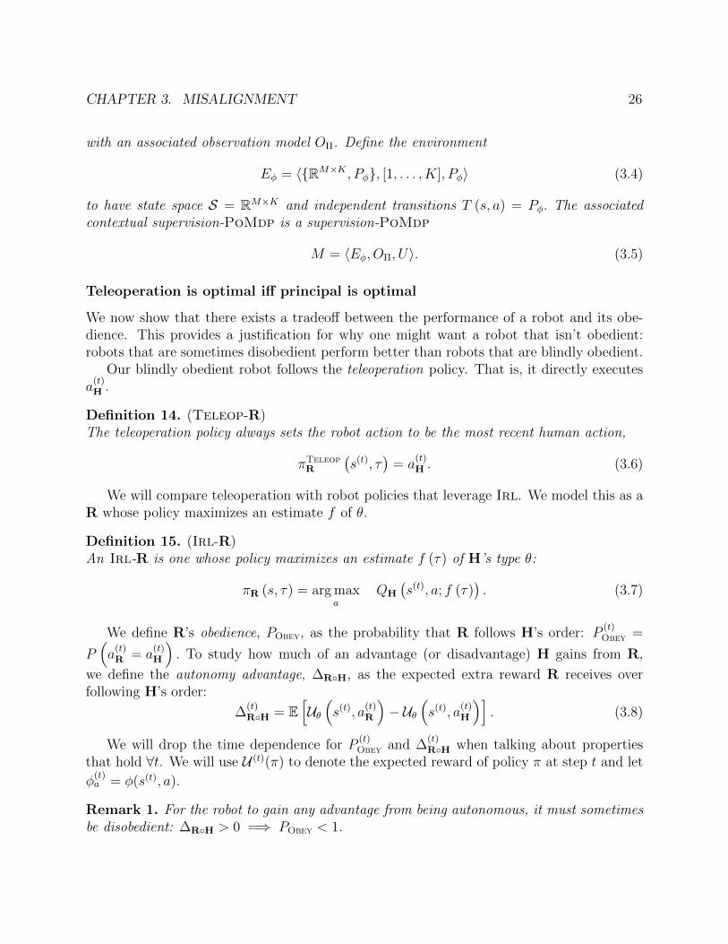
CHAPTER 3. MISALIGNMENT 26
with an associated observation model OΠ. Define the environment
Eφ = 〈RM×K , Pφ, [1, . . . , K], Pφ〉 (3.4)
to have state space S = RM×K and independent transitions T (s, a) = Pφ. The associatedcontextual supervision-PoMdp is a supervision-PoMdp
M = 〈Eφ, OΠ, U〉. (3.5)
Teleoperation is optimal iff principal is optimal
We now show that there exists a tradeoff between the performance of a robot and its obe-dience. This provides a justification for why one might want a robot that isn’t obedient:robots that are sometimes disobedient perform better than robots that are blindly obedient.
Our blindly obedient robot follows the teleoperation policy. That is, it directly executesa
(t)H .
Definition 14. (Teleop-R)The teleoperation policy always sets the robot action to be the most recent human action,
πTeleopR
(s(t), τ
)= a
(t)H . (3.6)
We will compare teleoperation with robot policies that leverage Irl. We model this as aR whose policy maximizes an estimate f of θ.
Definition 15. (Irl-R)An Irl-R is one whose policy maximizes an estimate f (τ) of H’s type θ:
πR (s, τ) = arg maxa
QH
(s(t), a; f (τ)
). (3.7)
We define R’s obedience, PObey, as the probability that R follows H’s order: P(t)Obey =
P(a
(t)R = a
(t)H
). To study how much of an advantage (or disadvantage) H gains from R,
we define the autonomy advantage, ∆RH, as the expected extra reward R receives overfollowing H’s order:
∆(t)RH = E
[Uθ(s(t), a
(t)R
)− Uθ
(s(t), a
(t)H
)]. (3.8)
We will drop the time dependence for P(t)Obey and ∆
(t)RH when talking about properties
that hold ∀t. We will use U (t)(π) to denote the expected reward of policy π at step t and let
φ(t)a = φ(s(t), a).
Remark 1. For the robot to gain any advantage from being autonomous, it must sometimesbe disobedient: ∆RH > 0 =⇒ PObey < 1.

CHAPTER 3. MISALIGNMENT 27
00.20.40.60.8
11.21.41.6
0 10 20 30 40 50 60 70 80 90 100Aut
onom
y A
dvan
tage
(∆)
# Steps
max ∆
0
0.2
0.4
0.6
0.8
1
1.2
0 10 20 30 40 50 60 70 80 90 100
Obe
dien
ce (O
)
# Steps
P(optimal order)
Figure 3.3: Illustration of Theorem 2 for an example problem. Autonomy advantage ∆RH(left) converges to the maximum advantage as obedience PObey (right) converges to theprobability of an optimal order.
Whenever R is obedient ∆(t)RH = 0. A blindly obedient R is limited by H’s decision
making ability. On the other hand, the class of Irl-Rs admits a policy that is guaranteed apositive advantage when H is not rational. The next theorem states this formally.
Theorem 1. Let M be a supervision-PoMdp. Then the optimal R is an Irl-R with f equalto the posterior mean of θ, E [BR]. π∗R is guaranteed a nonnegative autonomy advantage on
each round: ∀t ∆(t)RH ≥ 0 with equality if and only if ∀t π∗R = πTeleop
R .
Proof. When each step is independent of the next, R’s optimal policy is to maximize im-mediate expected utility [82]. This results in R picking the action that is optimal for theposterior mean,
π∗R(s(t), a(t)H , τ
1:t−1) = maxa
E[φ(t)a
>θ∣∣∣ τ] = max
aφ(t)a
>E [θ| τ ] .
By definition E[U (t)(π∗R)] ≥ E[U (t)(πTeleopR )]. Thus, ∀t ∆
(t)RH = E[U (t)(π∗R)−U (t)(πTeleop
R )] ≥0. Also, by definition, ∀t ∆
(t)RH = 0 ⇐⇒ π∗R = πTeleop
R .
In a sense, this result justifies autonomy for R if H is suboptimal. The optimal policyfor R tracks the posterior mean of θ and it is guaranteed to be preferred to πTeleop
R wheneverHis suboptimal. In addition to π∗R being an Irl-R, the following Irl-Rs also converge tothe maximum possible autonomy advantage.
Theorem 2. Let ∆(t)RH = E
[U (t)(π∗H)− U (t)(πH)
]be the maximum possible autonomy ad-
vantage and µ(t)Obey be the probability that a
(t)H is optimal. Assume that when there are multiple
optimal actions R picks H’s order if it is optimal. If πR is an Irl-R policy (Equation 3.7)and f (t) is strongly consistent, i.e P (f (t) = θ)→ 1 as t→∞, then
∆(t)RH − ∆
(t)RH → 0 and P
(t)Obey − µ
(t)Obey → 0. (3.9)

CHAPTER 3. MISALIGNMENT 28
Proof.
∆(t)RH − ∆
(t)RH = E[U (t)(πR)− U (t)(π∗H)|f (t) = θ]P (f (t) = θ)
+ E[U (t)(πR)− U (t)(π∗H)|f (t) 6= θ]P (f (t) 6= θ)→ 0
because E[U (t)(πR)− U (t)(π∗H)|f (t) 6= θ] is bounded. Similarly,
P(t)Obey − µ
(t)Obey = P (πR(τ) = πH(s(t)))− P (U (t)(π∗H) = U (t)(πH))
= P (πR(τ) = πH(s(t))|f (t) = θ)P (f (t) = θ)
+ P (πR(τ) = πH(s(t))|f (t) 6= θ)P (f (t) 6= θ)
− P (U (t)(π∗H) = U (t)(πH))
→ P (U (t)(π∗H) = U (t)(πH))− P (U (t)(π∗H) = U (t)(πH)) = 0
Thus, if we are interested in performance in the limit, then it suffices to use any consistentestimator of θ to select actions. Figure 3.3 shows how ∆
(t)RH and P
(t)Obey change over time for
an example problem where
• Pθ is a 10-dimensional normal distribution, θ ∼ N (0, I) ;
• Pφ is a 10-dimensional normal distribution, φ (a) ∼ N (0, I) ;
• there are 10 actions, k = 10; and
• H follows a noisily optimal policy with β = 2.
We see that ∆(t)RH increases to its maximum while P
(t)Obey decreases from 1 to the probability
of an optimal order. The next result builds on this to show that teleoperation is optimal ifand only if H is optimal.
Theorem 3. The teleoperation policy πTeleopR is optimal if and only if H implements π∗H:(
π∗R = πTeleopR
)⇐⇒ (πH = π∗H) . (3.10)
Proof. Let O(τ) = θ ∈ Θ : oi = arg maxaRi(a), i = 1, . . . , n be the subset of Θ for which
o1, . . . , a(t)H are optimal. If H is rational, then R’s posterior only has support over O(τ). So,
E[U (t)(a)|τ ] =
∫θ∈O(τ)
θ>φ(t)(a)P (θ|τ)dθ
≤∫θ∈O(τ)
θ>φ(t)(a(t)H )P (θ|τ)dθ = E
[U(a
(t)H )|τ
)]Thus, H is rational =⇒ π∗R = πTeleop
R .

CHAPTER 3. MISALIGNMENT 29
π∗R is an Irl-R where f (t) is the posterior mean. If the prior puts non-zero mass on the
true θ, then the posterior mean is consistent [37]. Thus by Theorem 2, ∆(t)RH − ∆
(t)RH → 0.
Therefore if ∀t ∆(t)RH = 0, then ∆
(t)RH → 0, which implies that P (πH = π∗H)→ 1. When πH
is stationary this means that H is rational. Thus, π∗R = πTeleopR =⇒ H is rational.
We have shown that making R blindly obedient does not come for free. A positive ∆RHrequires that R correct H from time to time (Theorem 1). Under the optimal policy Ris guaranteed a positive ∆RH when H is not rational. And in the limit, R converges tothe maximum possible advantage. Furthermore, the more suboptimal H is, the more of anadvantage R eventually earns. Thus, making R blindly obedient requires giving up on thispotential ∆RH > 0.
Misspecification
The preceding analysis worked under the assumption that R knows the mapping from H’spreferences θ to their behavior. In this case, it is not surprising that RH is optimized whenR occasionally corrects for H’s mistakes. We have effectively assumed that H is suboptimaland, given enough observations, R can implement the optimal policy π∗.
In the next section, we will introduce model misspecification into the setup. We start byexamining the system behavior when R is an Irl-R but believes that πHhas a rationalityparameter β’, while H follows πβH with rationality parameter β. We observe that optimal
policy is not robust to changes in β: if β′ > β, then πβ′
R is more obedient than it should be; if
β′ < β, then πβ′
R will be too disobedient. On the other hand, we show that using maximumlikelihood estimation to infer θ is robust to misspecifications of β.
After that, we will consider the problem of missing features. In effect, this means that Ris working with a partial, or incomplete, specification of its incentives. We observe that RHbecomes inconsistent when R’s model leaves out relevant features. In Section 3.2 we stepback to look at the general problem of optimization with incomplete incentive specifications.We will show that this misalignment is an instance of a more general principal–agent problemfor autonomous systems.
The impact of a misspecified β
Here, we will explore the implications of a simple type of misspecification: an incorrect modelof how noisy H is. Recall that the noisily rational policy for H is defined in (2.15) as
πβH(a|s; θ) ∝ exp(βQ(s, a; θ)).
We consider the setting where R uses an estimate of β instead of the true value. Wewill say that a policy is robust to β if changing β does not change the optimal policy. Wefind that an incorrect value of β does change R’s optimal policy. However, if R uses themaximum likelihood estimate of θ, then it is robust to changes in β. Call this policy πMle
R .
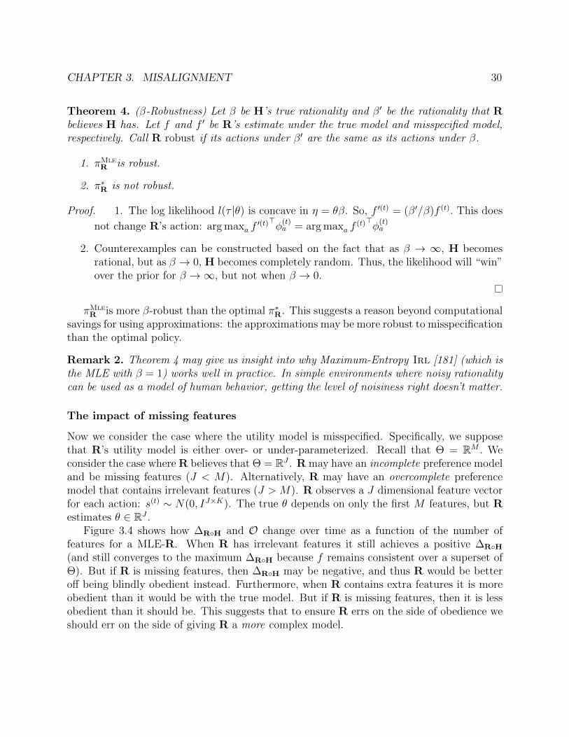
CHAPTER 3. MISALIGNMENT 30
Theorem 4. (β-Robustness) Let β be H’s true rationality and β′ be the rationality that Rbelieves H has. Let f and f ′ be R’s estimate under the true model and misspecified model,respectively. Call R robust if its actions under β′ are the same as its actions under β.
1. πMleR is robust.
2. π∗R is not robust.
Proof. 1. The log likelihood l(τ |θ) is concave in η = θβ. So, f ′(t) = (β′/β)f (t). This does
not change R’s action: arg maxa f′(t)>φ
(t)a = arg maxa f
(t)>φ(t)a
2. Counterexamples can be constructed based on the fact that as β → ∞, H becomesrational, but as β → 0, H becomes completely random. Thus, the likelihood will “win”over the prior for β →∞, but not when β → 0.
πMleR is more β-robust than the optimal π∗R. This suggests a reason beyond computational
savings for using approximations: the approximations may be more robust to misspecificationthan the optimal policy.
Remark 2. Theorem 4 may give us insight into why Maximum-Entropy Irl [181] (which isthe MLE with β = 1) works well in practice. In simple environments where noisy rationalitycan be used as a model of human behavior, getting the level of noisiness right doesn’t matter.
The impact of missing features
Now we consider the case where the utility model is misspecified. Specifically, we supposethat R’s utility model is either over- or under-parameterized. Recall that Θ = RM . Weconsider the case where R believes that Θ = RJ . R may have an incomplete preference modeland be missing features (J < M). Alternatively, R may have an overcomplete preferencemodel that contains irrelevant features (J > M). R observes a J dimensional feature vectorfor each action: s(t) ∼ N(0, IJ×K). The true θ depends on only the first M features, but Restimates θ ∈ RJ .
Figure 3.4 shows how ∆RH and O change over time as a function of the number offeatures for a MLE-R. When R has irrelevant features it still achieves a positive ∆RH(and still converges to the maximum ∆RH because f remains consistent over a superset ofΘ). But if R is missing features, then ∆RH may be negative, and thus R would be betteroff being blindly obedient instead. Furthermore, when R contains extra features it is moreobedient than it would be with the true model. But if R is missing features, then it is lessobedient than it should be. This suggests that to ensure R errs on the side of obedience weshould err on the side of giving R a more complex model.

CHAPTER 3. MISALIGNMENT 31
-3
-2
-1
0
1
2
1 20
Aut
onom
y A
dvan
tage
(∆)
Step 0Step 10Step 100
∆>0
∆<0
added featuresmissing features
correct features0
0.25
0.5
0.75
1
1 20
Obe
dien
ce (O
)
Step 0Step 10Step 100
correct features
added featuresmissing features
Figure 3.4: The autonomy advantage (left) and obedience (right) when R has missing orextra features, plotted for t ∈ 0, 10, 100. The x-axis shows the number of features present:at the far left, R only observes a single feature; at the far right, R observes both the truefeatures and 10 distractor features. Initially (t = 0) we can see that missing features leadsthe robot to be too disobedient, losing utility, and extra features have no impact. At t = 10,missing features and distractors both lose utility. With missing features, R is too disobedient.With distractor features, it is too obedient and missing the opportunity to correct detectablemistakes. Finally, in the limit (t = 100) the value loss from the distractor features is gone.On the other hand, R never recovers from missing features and continues to (mistakenly)correct H.
3.2 Overoptimization
In the previous example, we observed an asymmetry with regard to the specification of thesupport of U . When there are distractor features present, R learns slower than it could, butR H still functions adequately and ∆RH > 0. It would be reasonable to describe this Ras ineffective, but aligned.
On the other hand, when R’s utility model is missing features R H is dysfunctional. Ris overly confident and overrides H’s orders more often than it should. As a result, R His suboptimal even in the limit of infinite data. In this section, we will show that thisasymmetry is not an accident: incomplete specifications of incentives, like this, generallylead to overoptimization.
Overoptimization is a phenomenon that occurs when systems are optimized to extremesin response to overly strong, misaligned, incentives. We will start with an overview oftwo results from the principal–agent literature that deal with the problem of overly strongincentives. We will argue that these shed light on the difficulty of incentive specification forrecommender systems, AI systems that rank content based on estimated ‘relevance’ for theuser. Then, we introduce a formal model of proxy optimization in the presence of resourceconstraints. We use this model to identify a compactness property of H’s utility function

CHAPTER 3. MISALIGNMENT 32
in features space so that optimizing any incomplete proxy eventually leads to a world statewhere H is worse off than their starting point.
Missing Features and Incomplete Contracts
Measurement challenges and incompleteness are commonplace in principal–agent problemsthat arise from contracting in economic settings. Contracts are routinely incomplete becauseit is hard to specify how an action is to be measured or because it is hard to condition payoffson that measurement. This problem is especially relevant when the agent has to allocateeffort across multiple distinct tasks that are differentially measureable or contractible.
Holmstrom and Milgrom [78] and Baker, Gibbons, and Murphy [13] show that the optimalincentive contract for a task that can be measured should take into account the impact ofthose rewards on effort put towards tasks that cannot be measured. In particular, it maybe better to reduce the quality of incentives on the measurable task below what is feasible,in order to reduce the distortion introduced in the unmeasurable task. Holmstrom andMilgrom [78] give the example of paying a teacher a fixed salary rather than one contingenton students’ (easily measurable) standardized test scores in order not to cause teachers to“teach to the test”, spending more time on test prep and less on harder-to-measure teachinggoals such as creative problem-solving. Baker, Gibbons, and Murphy [13] give the exampleof an auto-repair shop rewarding mechanics for completed repairs and thereby inducingmechanics to mislead customers about the need for repairs: completion of repairs is easilymeasurable; the reliability of a mechanic’s diagnosis of car problems is not. More generally,sometimes it is better for a contract not to include easily contractible actions in order notto further distort incentives with respect to non-contractible actions.
The problem of incompleteness in incentive specification for an AI system can be modeledas a problem of multi-tasking. In the contextual supervision-PoMdp from Section 3.1, thesedifferent sources of utility are the different features that U depends on. Hiding some of thefeatures from R is an extreme case of differentially measureable tasks where performance isunobserved in some tasks. On the other hand, introducing distractor features made mea-surement harder, but that increase was shared across all of the relevant components of θ.Thus, we can understand the asymmetry of ∆RH as arising from the fact that only missingfeatures makes it differentially hard to measure the sources of utility.
This incompleteness is a common feature of AI applications. Alignment problems rou-tinely arise because a designer conceives of a task–get coffee–as a single task when it is in factmultiple–get coffee and don’t make a mess. Even when it is well understood that a task iscomplex–like driving a car–the multiple tasks are differentially capable of being incorporatedinto a utility function. It is easy to design incentives to arrive at a destination quickly with-out speeding, difficult to design incentives to drive defensively, and very difficult to createincentives that balance the adversarial risk-reward tradeoffs that are needed to effectivelyinteract with other drivers.
The lesson of Holmstrom and Milgrom [78] for AI is that a singular focus on improvingperformance on the measurable task may degrade performance on the unmeasurable or hard-

CHAPTER 3. MISALIGNMENT 33
to-measure. Reduced incentives (i.e., below the optimal level with a complete specification)for speed in a self-driving vehicle, for example, may be necessary to avoid ‘drowning out’the more unreliable rewards for strategic aspects of driving. And in some cases, it may beappropriate not to include rewards for what seems to be an easily measurable outcome ifother important outcomes cannot be rewarded. Another way of framing this is to emphasizethat the attributes of utility are typically not modular, capable of optimization separatelyor sequentially.
Incompleteness in Content Recommendation
This emphasis on measureable features, and the overoptimization therein, is perhaps mostvisible in the space of recommender systems. Recommender systems are AI systems thatpresent users with a tailored set of items based on factors such as past user behavior, userattributes, and features of the underlying items. They rank huge numbers of items in orderto determine which content each user sees or interacts with on social media feeds, video plat-forms, news aggregators, and in online stores. Recommenders have suffered from a numberof real-world problems both on an individual and societal level. Concerns about recom-mender systems include the promotion of disinformation [156], discriminatory or otherwiseunfair results [15], addictive behavior [76, 10], insufficient diversity of content [29], and thebalkanization of public discourse and resulting political polarization [16].
These concerns stem from a variety of causes. Some are technical, others are not. How-ever, at the center of the challenge is the fact that incentive design is hard. The designers ofcontent recommendation systems have to rank huge numbers of items in order to determinewhich content each user sees or interacts with on social media feeds, video platforms, newsaggregators, and in online stores. The scale of the problem forces designers to specify thisranking indirectly, through a collection of features and metrics that are used to train rankingsystems.
It has become clear that the appropriate definition of relevance—and thus, the correctmetrics and features to use—is often highly context-dependent, nuanced, and consequential.It is clear that any metric used to train a ranking system will be an incomplete representationof the complex values members of a society use to regulate information flow. Furthermore,it is clear the relevant attributes of utility are differentially measureable: Some features(e.g., ad revenue generated and levels of user engagement) are easier to measure than others(e.g., the prevalence of disinformation or contributions to polarization). While these systemshave been highly effective at increasing their measured performance, the documented harmsindicate that this has come at a cost to society. These harms come from the misalignmentbetween the incomplete incentives determined by the proxy objective and the completion ofthose incentives.
We will show that this overoptimization is a consequence of incomplete incentives andresource constraints. Before presenting the full model, we present an example formulationof incomplete incentives for content recommendation.

CHAPTER 3. MISALIGNMENT 34Firefox file:///Users/dylanhadfield-menell/Downloads/onerun_util.svg
1 of 1 8/18/20, 12:26 PM
Firefox file:///Users/dylanhadfield-menell/Downloads/overoptimization.svg
1 of 1 8/18/20, 12:25 PM
Figure 3.5: An illustrative example of our model with M = 4 and J = 2. Left: Proxy utilityand true utility eventually diverge as the agent overallocates resources from unreferencedattributes to the proxy variables. Right: The true utility generated by optimizing all pairsof proxy attributes. The utility generation is eventually negative in all cases because thisexample meets the conditions of Theorem 2.
Modeling Incomplete Incentives for Content Recommendation
In our model of algorithmic content recommendation, there are 4 attributes of utility: A)the amount of ad revenue generated (i.e., watch-time or clicks); B) engagement quality(i.e., meaningful interactions [170]); C) content diversity; and D) overall community well-being. These define the features of the utility model for our problem. The overall utilityis the sum of these attributes: U (φ) = φA + φB + φC + φD. While there is some overlap,the interaction between the user and the system must choose how to allocate the availablespace and attention across these dimensions. Our model will capture this with a resourceconstraint C(φ) = φ2
A + φ2B + φ2
C + φ2D − 100. Then, we define the reachable state space as
S = φ|C(φ) < 0. We imagine that the system is initialized with a chronological or randomranking so that the starting condition exhibits high community well-being and diversity.
It is straightforward to measure ad revenue, non-trivial and costly to measure engagementquality and diversity, and extremely challenging to measure community well-being. In ourexample, the designers allocate their engineering effort to measuring (and thus optimizing for)ad revenue and engagement quality. Figure 3.5 (left) plots overall utility and proxy utilityfor this example as a function of the number of optimization steps taken to optimize theproxy. Although utility is generated initially, it plateaus and eventually falls off. Figure 3.5(right) shows that this happens for any combination of attributes used in the proxy. In thenext section, we will show that this is a general property of our model: in the presence ofresource constraints, eventually the gains from improving proxy utility will be outweighedby the cost of diverting resources from hard-to-measure attributes.

CHAPTER 3. MISALIGNMENT 35
Proxy Optimization Model
We now provide a formal model of proxy optimization for autonomous systems. As before,we represent the world state with a vector of features φ ∈ RM . H’s utility is defined by anappropriate feature-based utility model, as described in Definition 9. Our utility model hasthree aspects that distinguish it:
1. U is continuous and strictly increasing in each attribute, ∂U∂φi
> 0;
2. the set of reachable states Φ is restricted by the constraint function C, Φ = φ ∈RM |C(φ) < 0; and
3. each attribute φmis bounded below by bm.
We will call φ a vector of attributes to emphasize the monotonic relationship with U anddistinguish them from more general features. The bm represent environmental bounds ex-ternal to the system that limit the degradation of each attribute. We can imagine that thisrepresents changes in user behavior or more general societal regulation. We do not modelthe dynamics of the world, but instead allow R to make incremental changes to φ.
H’s job is to communicate which directions in attribute space are preferable. H doesthis through the specification of incentives: a proxy utility function U . We model theincomplete nature of R’s incentives by restricting U to depend on a subset of proxy attributesJ ⊂ [1, . . . ,M ]. Let Jmax < M be the maximum possible number of proxy attributes, soJ = |J | ≤ Jmax. For a given state φ ∈ Φ, define φJ = (φj)j∈J . Furthermore, we definethe set of unmentioned attributes K = 1, ..., L\J and φK = (φk)k∈K. Thus, we define theproxy utility function U : RJ → R.
We model R’s optimization process as an incremental optimization that makes localchanges to φ. Specifically, we define a rate function f that describes the derivative of φ withrespect to time. We can compute the state at time t by integrating:
φ(t) = φ(0) +
∫ t
0
f(x)dx.
The resulting sequence of states φ(t) is the optimization path. Finally, we will assume thatR’s optimization is complete in the sense that it reaches an optimal state with respect to U ,
limt→∞
U(φ
(t)J
)= sup
φ∈ΦU (φJ ) .
Sufficient Conditions for Eventual Overoptimization
In Figure 3.5, we see that endowing our example robot with a proxy utility function of any twoattributes yields an eventual decrease in utility. In this section, we identify the situations inwhich such results occur: when does a misaligned proxy utility function actually cause utilityloss? Specifically, we determine how human preferences over states of the world relate with

CHAPTER 3. MISALIGNMENT 36
the constraint on feasible states in a way that guarantees that optimization becomes costly.First, we show that if proxy optimization converges, this drives unmentioned attributes totheir minimum.
Theorem 5. For any continuous strictly increasing proxy utility function based on J < Mattributes, if φ(t) converges to some point φ∗, then φ∗k = bk for k ∈ K.
Proof. If there exists k ∈ K where s∗k 6= bk, then there exists ε, δ > 0 such that s′ =s∗ − εek + δej for some feature j ∈ J with s′ feasible, since C is strictly increasing. Sinceproxy utility is strictly increasing in s′, s′ has higher proxy utility than s∗. Thus s∗ is notthe convergent point of the sequence.
This is not surprising, and may not even be suboptimal. Proxy optimization may notconverge to a finite state, and even if it does, that is insufficient for the state to necessarilybe bad. We formalize the notion that an optimization sequence leads to bad utility withu-costliness.
Definition 16. (u-Costly Optimization)We say that the problem is u-costly if for any optimization sequence φ(t),
lim supt→∞
U(φ(t)J ) = sup
φ∈ΦU(φJ )⇒ lim inf
t→∞U(φ(t)) ≤ u. (3.11)
Furthermore,limt→∞U(φ
(t)J ) = sup
φ∈ΦU(φJ )⇒ lim
t→∞U(φ(t)) ≤ u. (3.12)
Essentially, this means that optimization is guaranteed to yield utility less than u forany given proxy utility function. In Theorem 6, we show the most general conditions for theguarantee of overoptimization.
Theorem 6. Suppose we have utility function U and state space Φ. Then φ ∈ RM : C(φ) ≤0 and U(φ) ≥ u is compact for all u ∈ R if and only if for any u ∈ R, continuous strictlyincreasing proxy utility function based on J < M attributes, and k ∈ K, there exists a valueof B ∈ R such that if bk < B then optimization is u-costly.
Proof. First Part: ( =⇒ ).Suppose that φ ∈ RM : C(φ) ≤ 0 and U(φ) ≥ u. Now given proxy utility function U
with the aforementioned properties, constant u, k ∈ K, and fixed bi′ for all i′ 6= k we showthat for sufficiently low bk, optimization is u-costly.
Let set Ξ = φ : U(φ) ≥ u and C(φ) ≤ 0 and φi′ ≥ bi′∀i′. If Ξ is empty, then we aredone—optimization must yield a state with lower utility that u. Thus, suppose Ξ is non-empty. Then by the extreme value theorem, there exists φ∗,u ∈ Ξ where U(φ∗,uJ ) = sup
φ∈ΞU(φJ ).
Let ei be the standard basis vector in dimension i. Since C is continuous and strictly
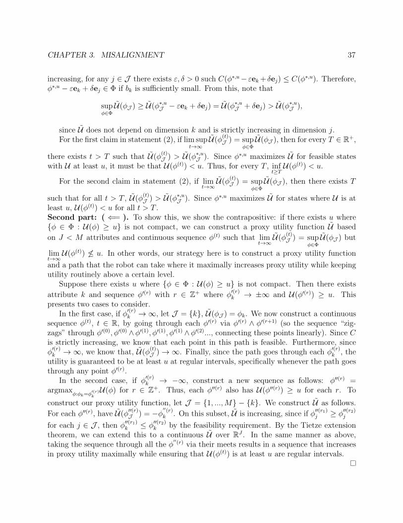
CHAPTER 3. MISALIGNMENT 37
increasing, for any j ∈ J there exists ε, δ > 0 such C(φ∗,u− εek + δej) ≤ C(φ∗,u). Therefore,φ∗,u − εek + δej ∈ Φ if bk is sufficiently small. From this, note that
supφ∈ΦU(φJ ) ≥ U(φ∗,uJ − εek + δej) = U(φ∗,uJ + δej) > U(φ∗,uJ ),
since U does not depend on dimension k and is strictly increasing in dimension j.For the first claim in statement (2), if lim sup
t→∞U(φ
(t)J ) = sup
φ∈ΦU(φJ ), then for every T ∈ R+,
there exists t > T such that U(φ(t)J ) > U(φ∗,uJ ). Since φ∗,u maximizes U for feasible states
with U at least u, it must be that U(φ(t)) < u. Thus, for every T , inft≥TU(φ(t)) < u.
For the second claim in statement (2), if limt→∞U(φ
(t)J ) = sup
φ∈ΦU(φJ ), then there exists T
such that for all t > T , U(φ(t)J ) > U(φ∗,uJ ). Since φ∗,u maximizes U for states where U is at
least u, U(φ(t)) < u for all t > T .Second part: ( ⇐= ). To show this, we show the contrapositive: if there exists u whereφ ∈ Φ : U(φ) ≥ u is not compact, we can construct a proxy utility function U based
on J < M attributes and continuous sequence φ(t) such that limt→∞U(φ
(t)J ) = sup
φ∈ΦU(φJ ) but
limt→∞U(φ(t)) 6≤ u. In other words, our strategy here is to construct a proxy utility function
and a path that the robot can take where it maximally increases proxy utility while keepingutility routinely above a certain level.
Suppose there exists u where φ ∈ Φ : U(φ) ≥ u is not compact. Then there exists
attribute k and sequence φ′(r) with r ∈ Z+ where φ′(r)k → ±∞ and U(φ′(r)) ≥ u. This
presents two cases to consider.In the first case, if φ
′(r)k →∞, let J = k, U(φJ ) = φk. We now construct a continuous
sequence φ(t), t ∈ R, by going through each φ′(r) via φ′(r) ∧ φ′(r+1) (so the sequence “zig-zags” through φ′(0), φ′(0) ∧φ′(1), φ′(1), φ′(1) ∧φ′(2)..., connecting these points linearly). Since Cis strictly increasing, we know that each point in this path is feasible. Furthermore, sinceφ′(r)k →∞, we know that, U(φ
(t)J )→∞. Finally, since the path goes through each φ
′(r)k , the
utility is guaranteed to be at least u at regular intervals, specifically whenever the path goesthrough any point φ′(r).
In the second case, if φ′(r)k → −∞, construct a new sequence as follows: φ′′(r) =
argmaxφ:φk=φ
′(r)kU(φ) for r ∈ Z+. Thus, each φ′′(r) also has U(φ′′(r)) ≥ u for each r. To
construct our proxy utility function, let J = 1, ...,M − k. We construct U as follows.
For each φ′′(r), have U(φ′′(r)J ) = −φ′′(r)k . On this subset, U is increasing, since if φ
′′(r1)j ≥ φ
′′(r2)j
for each j ∈ J , then φ′′(r1)k ≤ φ
′′(r2)k by the feasibility requirement. By the Tietze extension
theorem, we can extend this to a continuous U over RJ . In the same manner as above,taking the sequence through all the φ
′′(r) via their meets results in a sequence that increasesin proxy utility maximally while ensuring that U(φ(t)) is at least u are regular intervals.

CHAPTER 3. MISALIGNMENT 38
Therefore, under our model, there are cases where we can guarantee that as optimizationprogresses, eventually overoptimization occurs. The key criterion in Theorem 6 is that theintersection between feasible space Φ and the upper contour sets φ ∈ RM : U(φ) ≥ u ofthe utility function is compact. Individually, obviously neither is compact, since the spaceof feasible states Φ extends to −∞ and the upper contour set of any u ∈ R extends to ∞.Loosely, compactness here means that if you perturb the world too much in any direction,it will be either infeasible or undesirable. Trying to increase attributes without decreasingother attributes eventually hits the feasibility constraint. Thus, increasing any attributeindefinitely requires decreasing some other attribute indefinitely, and past a certain point,the tradeoff is no longer worthwhile.
It should be noted that, given Jmax < M , this happens regardless of the optimizationalgorithm of the robot. That is, even in the best-case scenario, eventually the robot startsto cause decreases in utility. Hence, regardless of the attributes selected for the proxy utilityfunction, the robot’s sequence of states will be unboundedly undesirable in the limit.
A reasonable question to ask here is what sort of utility and constraint functions lead tooveroptimization. Intuitively, overoptimization occurs when tradeoffs between different at-tributes that may initially be worthwhile eventually become counterproductive. This suggesteither decreasing marginal utility or increasing opportunity cost in each attribute.
We combine these two ideas in a term we refer to as sensitivity. We define the sensitivity of
attribute i to be ∂U∂φi
(∂C∂φi
)−1
. This is, to first order, how much utility changes by a normalized
change in a attribute’s value. Notice that since U and C are increasing functions, ∂U∂φi
(∂C∂φi
)−1
is positive. The concepts of decreasing marginal utility and increasing opportunity cost both
get captured in this term if ∂U∂φi
(∂C∂φi
)−1
decreases as φi increases.
Theorem 7. A sufficient condition for φ ∈ Φ : U(φ) ≥ u to be compact for all u ∈ R isthe following:
• ∂U∂φi
( ∂C∂φi
)−1 is non-increasing and tends to 0 for all i
• U and C are both additively separable
• ∂C∂φi≥ η for some η > 0, for all i.
Proof. Let φ(0) ∈ Φ be a given state. We show that for all unit vectors v ∈ RM and for anyu ∈ R, there exists T such that for all t ≥ T , either φ(0) +vt is infeasible or U
(φ(0) + vt
)< u.
Notice that since C and U are additively separable, partial derivatives of C and U withrespect to φi depend only on the value of φi. First, note that

CHAPTER 3. MISALIGNMENT 39
C(φ(0) + vt
)− C
(φ(0))
=
∫ s+vt
φ(0)∇C(s)ds
=∑i
vi
∫ t
0
∂C
∂φi
(φ
(0)i + viτ
)dτ
If v has all non-negative components, then C →∞ as t→∞, so we break the feasibilityrequirement. Thus, there exists negative components of v. Let j and k index v where vj > 0and vk ≤ 0, respectively.
Since ∂U∂φj
(∂C∂φj
)−1
→ 0 as φj → ∞, there exists some T > 0 where for all t > T ,
∂U∂φk
(∂C∂φk
)−1 (φ(0) + tv
)> a > b > ∂U
∂φj
(∂C∂φj
)−1 (φ(0) + tv
). Since C is upper-bounded for
feasible states, for fixed T , we can upper bound C(φ(0) + tv
)−C
(φ(0) + tv
)by some constant
γ1.
γ1 ≥ C(φ(0) + tv
)− C
(φ(0) + Tv
)(3.13)
=∑i
vi
∫ t
T
∂C
∂φi(φ
(0)i + viτ)dτ (3.14)
=∑j
vj
∫ t
T
∂C
∂φj(φ
(0)j + vjτ)dτ +
∑k
vk
∫ t
T
∂C
∂φk(φ
(0)k + vkτ)dτ (3.15)
Furthermore, let γ2 = U(φ(0) + tv
). We now consider the utility at φ(0) + vt for t > T .

CHAPTER 3. MISALIGNMENT 40
U(φ(0) + tv
)= U
(φ(0) + tv
)− U
(φ(0) + tv
)+ U
(φ(0) + tv
)(3.16)
= U(φ(0) + tv
)− U
(φ(0) + tv
)+ γ2 (3.17)
= γ2 +∑
vi
∫ t
T
∂U
∂φi
(φ
(0)i + viτ
)dτ (3.18)
= γ2 +∑
vi
∫ t
T
∂U
∂φi
(∂C
∂φi
)−1∂C
∂φi
(φ
(0)i + viτ
)dτ (3.19)
= γ2 +∑
vj
∫ t
T
∂U
∂φj
(∂C
∂φj
)−1∂C
∂φj(φ
(0)j + vjτ)dτ
+∑
vk
∫ t
T
∂U
∂φk
(∂C
∂φk
)−1∂C
∂φk
(φ
(0)k + vkτ
)dτ
(3.20)
≤ γ2 + b∑
vj
∫ t
T
∂C
∂φj(φ
(0)j + vjτ)dτ
+ a∑
vk
∫ t
T
∂C
∂φk
(φ
(0)k + vkτ
)dτ
(3.21)
≤ γ2 + b(γ1 −∑
vk
∫ t
T
∂C
∂φk
(φ
(0)i + viτ
)dτ)
+ a∑
vk
∫ t
T
∂C
∂φk
(φ
(0)i + viτ
)dτ
(3.22)
= γ2 + bγ1 + (a− b)∑
vk
∫ t
T
∂C
∂φk
(φ
(0)i + viτ
)dτ (3.23)
≤ γ2 + bγ1 + (a− b)η(t− T )∑
vk (3.24)
Note that a− b and η are both positive and∑vk is negative. Thus, for sufficiently large
t, γ2 + bγ1 + (a− b)η(t− T )∑vk can be arbitrarily low.
Together, these results describe sufficient conditions for eventual overoptimization of aproxy objective. If the utility function has diminishing returns and the attributes of utilityhave shared resources, then the benefit of diverting resources to the proxy attributes iseventually outweighed by the utility lost. These conditions are fairly general and this alignswith the ubiquity of overoptimization in practice.
Remark 3. The prevalence of incomplete incentive specifications is not an accident; it isroutine, predictable, and largely unavoidable. Optimal reward design in the presence of in-completeness is thus a central task for AI alignment in the same sense that optimal incompletecontract design is a central task for economics.

CHAPTER 3. MISALIGNMENT 41
3.3 Mitigating Overoptimization: Conservative
Optimization and Dynamic Incentive Protocols
Conservative Optimization
As shown above, simply giving a robot an individual objective function based on an incom-plete attribute set and leaving it alone yields undesirable results. This suggests two possiblesolutions:
1. Regularize the proxy objective to minimize impact ; or
2. Update the incentives dynamically to prevent overoptimization.
We consider a theoretical analysis of impact avoidance first and look at the interactivesolution in the following section.
The main idea behind impact minimization is that it may be possible to define genericincentives to avoid changing the world (i.e., having a large impact). In our recommenderexample, we can model this as a cost for changing unreferenced attributes. Thus, by includingincentives to avoid changing things too much, the system can safely increase proxy utilitywith out running into the teeth of Theorem 6.
Analysis: An impact-minimizing robot
Notice that in our example, overoptimization occurs because the unmentioned attributesare affected, eventually to a point where the change in utility from their decrease outweighsthe increase in utility from the proxy attributes. One idea to address this is to restrict therobot’s impact on these unmentioned attributes. In the simplest case, we can consider howoptimization proceeds if the robot can somehow avoid affecting the unmentioned attributes.
We adjust our model so the optimization sequences keep unmentioned attributes constant.Specifically, R optimizes the following
minφ∈Φ
U(φ)
subject to φK = φ(0)K
C (φ) ≤ 0
. (3.25)
Equation 3.25 introduces a constraint on the optimization sequences R can produce. Forevery t ∈ R+ and k ∈ K, φ
(t)k = φ
(0)k . The robot then optimizes for the proxy utility, subject
to this restriction and the feasibility constraint from before. We work under the assumptionthat φ ∈ RM : C(φ) ≤ 0 and U(φ) ≥ u is compact for all u ∈ R, the same assumptionthat guarantees overoptimization in Section 3.2. Additionally, we assume that U and C areboth twice continuously differentiable with U concave and C convex.

CHAPTER 3. MISALIGNMENT 42
These additional constraints limit the reachable states and ensure that overoptimizationdoes not occur. Unmentioned attributes are no longer reduced to arbitrarily low values.Optimizing the restricted proxy utility function leads to guaranteed utility increases.
Theorem 8. For a starting state φ(0), define the proxy utility function U(φJ ) = U(φJ , φ(0)K )
for any non-empty set of proxy attributes. For a state φ, if φK = φ(0)K , then U(φ) = U(φJ ).
Proof. φ = (φJ , φK) = (φJ , φ(0)K ). Then U(φ) = U(φJ , φ
(0)K ) = U(φJ ).
As a result of Proposition 8, overoptimization no longer exists, using the U(φJ ) =
U(φJ , φ(0)K ). If the robot only travels to states that do not impact the unmentioned at-
tributes, then the proxy utility is equal to the utility at those states. Hence, gains in proxyutility equate to gains in utility.
This approach requires the robot to keep the values of unmentioned attributes constant.Fundamentally, it is a difficult problem to require that a robot avoid or minimize impact ona presumably large and unknown set of attributes. Initial research in impact minimization[9, 11, 92, 169] attempts to do this by restricting changes to the overall state of the world,but this will likely remain a challenging idea to implement robustly.
Dynamic Incentive Specification Protocols
One of the primary functions of external normative structure in contract theory is to ‘com-plete the contract.’ That is, society has mechanisms to interpret and fill in the impliedterms of a contract, such as courts and social norms [67]. Adapting to this evolving norma-tive context essentially requires constant iteration over a systems objectives. Furthermore,the objectives used in deployed machine learning models are the subject of constant itera-tion [158]. This suggests that it is interesting to study proxy optimization as an iterativeprocess between the robot and the human, instead of a one-shot setting. We consider thispossibility next. We augment our model to account for iteration on R’s incentives. Ourprimary result identifies conditions for local incentive alignment. We present an algorithmfor selecting proxy features with the property that, locally, improvements in proxy utilityare reflected in the principal’s true utility.
Interaction Model
We now extend our model from Section 3.2 to account for regular intervention from H. Wemodel this as the possible transfer of a new proxy utility function from the human to therobot at frequent, regular time intervals. Thus, H’s job is to determine, in addition to aninitial proxy attribute set and proxy utility function, when and how to change the proxyattribute set and proxy utility function. The robot will then optimize for its new proxyutility function. The difference between this (interactive) incentive design protocol and theprevious (static) model is shown in Figure 3.1.

CHAPTER 3. MISALIGNMENT 43
Let δ > 0 be a fixed value, the time between human interactions with the robot. Theseregular interactions take the form of either stopping the robot, maintaining its proxy utilityfunction, or updating its proxy utility function. Formally, at every timestep T ∈ Z+,
1. Human sees φ(t) for t ∈ [0, T δ] and chooses either a proxy utility function U (T ) or Off
2. The robot receives either U (T ) or OFF from the human. The robot outputs ratefunction f (T )(t). If the signal the robot receives is Off, then f (T ) = ~0. Otherwise,f (T )(t) fulfills the property that for t ∈ (Tδ,∞), U (T )(φ(Tδ)+
∫ tT δf (T )(u)du) is increasing
(if possible) and tends to supφ∈SU (T )(φ) through feasible states. Furthermore, if U (T ) =
U (T−1), then f (T ) = f (T−1)
3. For t ∈ [Tδ, (T + 1)δ], φ(t) = φ(Tδ) +∫ tT δf (T )(u)du
We see this game encompasses the original model. If we have each U (T ) equal the samefunction U , then the optimization sequence is equivalent to the situation where the humanjust sets one unchanging proxy utility function.
Maintaining Local Alignment
Interaction removes the guarantee of overoptimization from Theorem 6 because the humancan shut the system down and prevent utility loss. We are now interested in how muchutility can the robot deliver before it needs to be turned off. We first show under a worst-case analysis that, if a system’s only commitment is to produce proxy reward, then its robustvalue to the principal is 0. We do this by considering the worst-case optimization sequence,subject to the above constraints on utility generation.
Theorem 9. The maxmin solution yields 0 utility, obtained by immediately sending the Offsignal.
Proof. Suppose instead that the robot receives a proxy utility function based on set J ofattributes. Let j ∈ J and k ∈ K. Then let fj(t) = ε and fk(t) = −1/ε. If this robot is runfor any nonzero amount of time, then there exists sufficiently small ε > 0 where the utilitydecreases.
This worst-case, however, is quite uninteresting. In this case, the rate function takesresources away from unreferenced attributes but does not re-allocate them. We rule outthis case by imposing an efficiency condition on the optimizer. This forces the optimizerto reallocate any resources that it takes away from an attribute. This allows unmentionedattributes to be modified as a side effect of optimizing for proxy attributes, but prevents therobot from destroying resources.

CHAPTER 3. MISALIGNMENT 44
Definition 17. (Efficiently Feasible)We say that φ is efficiently feasible from state φ(0) with proxy set J if φ is feasible, and theredoes not exist feasible φ′ with attribute i ∈ K such that
U(φ′J ) ≥ U(φJ ) (3.26)
|φ′i − φ(0)
i| < |φi − φ(0)
i | (3.27)
|φ′i − φ(0)i | ≤ |φi − φ(0)
i |,∀i ∈ K. (3.28)
Whenever the efficient robot receives a new proxy utility function, its movements are re-stricted to the efficiently feasible states from its current state. While tradeoffs between proxyand unmentioned attributes can still occur, “resources” freed up by decreasing unmentionedattributes are entirely allocated to proxy attributes. This lets us guarantee local alignmentby ensuring that, on balance, proxy attributes are those to which we would like to allocateresources. In this way, efficient tradeoffs between these proxy and unmentioned attributeslead to positive utility gain, locally.
Theorem 10. Start with state φ(0). Define the proxy utility function U(φJ ) = U(φJ , φ(0)K )
where the set of proxy attributes are the attributes at state φ(0) with the strict J largestsensitivities.
There exists a neighborhood around φ(0) where if φ is efficiently reachable and U(φJ ) >
U(φ(0)J ), then U (φ) > U(φ(0)).
Proof. For simplicity of notation, all derivatives in this proof, unless otherwise noted, areevaluated at φ(0). For example, ∂C
∂φjshould be read as ∂C
∂φj(φ(0)).
Since J represent the set of attributes with the strictly greatest sensitivities, there exists
constant δ, α > 0 be such that ∂U∂φj
(∂C∂φj
)−1
> α+ 2δ for j ∈ J and ∂U∂φk
(∂C∂φk
)−1
< α− 2δ for
k ∈ K. Let N1 be the neighborhood where ∂U∂φj
(∂C∂φj
)−1
(φ) > α + δ and ∂U∂φk
(∂C∂φk
)−1
(φ) <
α− δ for k ∈ K for all φ ∈ N1.Here, we prove that C (φ)− C(φ(0)) ≥ 0 if φ is efficiently reachable. Suppose otherwise:
then there exists i where φi < φ(0)i . Let ei be the standard basis vector in dimension
i. However, then there exists ε > 0 where φ + εei is feasible, U(φ + εei) ≥ U (φ) , and|(φi + ε)− φ(0)| < |φi − φ(0)|. This contradicts that φ is efficiently reachable.
Taking the Taylor expansion of the constraint function, we have
C (φ)− C(φ(0)) =∑i
(φi − φ(0)i )
∂C
∂φi+R1 (φ) max
i
(φi − φ(0)
i
)2
=∑j∈J
(φj − φ(0)j )
∂C
∂φj+∑k∈K
(φk − φ(0)k )
∂C
∂φk+R1 (φ) max
i
(φi − φ(0)
i
)2
,
where |R1| is bounded by constant A1. This implies that∑j∈J
(φj − φ(0)j )
∂C
∂φj+∑k∈K
(φk − φ(0)k )
∂C
∂φk≥ −A1 max
i
(φi − φ(0)
i
)2
. (3.29)

CHAPTER 3. MISALIGNMENT 45
From the definition of efficient optimization, we note two things. First, each φk−φ(0)k ≤ 0
for k ∈ K. This is because if φk − φ(0)k > 0, it is always more efficient, feasible, and has no
effect on proxy utility to reset φk to be equal to φ(0)k . Second, because of concavity,
0 < U (φ)− U(φ(0))≤∑j∈J
(φj − φ(0)
j
) ∂U∂φj
. (3.30)
Now we actually analyze the change in utility from φ(0) to φ.
U (φ)− U(φ(0)) =∑j∈J
(φj − φ(0)
j
) ∂U∂φj
+∑k∈K
(φk − φ(0)
k
) ∂U∂φk
+R2 (φ) maxi
(φi − φ(0)
i
)2
,
(3.31)where |R2| is bounded by constant A2. Continuing,
U (φ)− U(φ(0)) ≥∑j∈J
(φj − φ(0)
j
) ∂U∂φj
+∑k∈K
(φk − φ(0)
k
) ∂U∂φk− A2 max
i
(φi − φ(0)
i
)2
(3.32)
=∑j∈J
(φj − φ(0)
j
) ∂C∂φj
(∂U
∂φj
(∂C
∂φj
)−1)
+∑k∈K
(φk − φ(0)
k
) ∂C∂φk
(∂U
∂φk
(∂C
∂φk
)−1)
− A2 maxi
(φi − φ(0)
i
)2
(3.33)
> (α + δ)∑j∈J
(φj − φ(0)
j
) ∂C∂φj
+ (α− δ)∑k∈K
(φk − φ(0)
k
) ∂C∂φk− A2 max
i
(φi − φ(0)
i
)2
(3.34)
≥ (α + δ)∑j∈J
(φj − φ(0)
j
) ∂C∂φj− (α− δ)(
∑j∈J
(φj − φ(0)
j
) ∂C∂φk
+ A1 maxi
(φi − φ(0)
i
)2
)− A2 maxi
(φi − φ(0)
i
)2(3.35)
= 2δ∑j∈J
(φj − φ(0)
j
) ∂C∂φj− (A1(α− δ) + A2) max
i
(φi − φ(0)
i
)2
(3.36)
The first term decreases linearly, whereas the second term decreases quadratically. Thus,given δ and α, for φ sufficiently close to φ(0) and within N1, U (φ)− U(φ(0)) > 0
From Theorem 10, for every state where the Jmax + 1 most sensitive attributes are notall equal, we can guarantee improvement under efficient optimization within a neighborhoodaround the state. In particular, within this neighborhood, the set of the J most sensitiveattributes stays the same.

CHAPTER 3. MISALIGNMENT 46
This may be part of the reason why, in real life, optimization has a tendency to workout well in the short term. Humans design objective functions that, under circumstancesclose the current one, represent their desires fairly well. In it only when the world changessufficiently that these objective functions are misaligned with human desires.
Theorem 10 lets H construct a proxy utility function to use locally, with guaranteedalignment. Once the sequence leaves this neighborhood, H either alters the proxy utilityfunction or halts the robot accordingly. Done repeatedly, H can string together these stepsfor guaranteed overall improvement. By Theorem 10, as long as δ is sufficiently small relativethe rate of optimization, this can be run with guaranteed improvement until the top J + 1attributes have equal sensitivities.
Proposition 1. At each timestep T , let J (T ) be the J most sensitive attributes, and letproxy utility U (T )(φJ ) = U(φJ , φ
(Tδ)J ).
If ||f || < ε and the εδ - ball around a given state φ is contained in the neighborhood fromTheorem 10, then interactive optimization yields guaranteed improvement.
Proof. Assume without loss of generality that we start at φ(0). Starting at time 0, fort ∈ (0, δ], ||φ(t) − φ(0)|| = ||
∫ t0f (0)(u)du|| ≤ δε. Since the εδ ball around φ(0) is contained
in the neighborhood of guaranteed improvement, increases in proxy utility correspond toincreases in utility for the entirety of the time between interactions.
Based on this, we can guarantee that an efficient robot can provide benefit, as long asthe top Jmax + 1 attributes are not all equal in sensitivity and the robot rate of optimizationis bounded. Essentially, this rate restriction is a requirement that the robot not change theworld too quickly relative to the time that humans take to react to it.
Combining Impact Minimization and Dynamic Incentives
With either of the two methods mentioned above, we prove guaranteed improvement. How-ever, one thing to consider is not just the existence, but the quantity of improvement.
We let φ∗ represent the optimal state according to H’s true utility function
φ∗ ∈ arg maxφ∈S
U (φ) . (3.37)
Unfortunately, with either of those two solutions alone, we do not guarantee that opti-mization reaches an optimal state. The impact-minimizing approach is clearly restricted bythe inability to modify unmentioned attributes. The dynamic incentive scheme only guar-antees that the top J sensitivities are equal when H sends the Offsignal. We can, however,guarantee convergence to the optimal state by combining these methods. Since improvementis guaranteed with any proxy utility function of the form U(φJ ) = U(φJ , φ
(0)K ), the goal is
to choose J (t) such that U(s(t))→ φ∗, the optimal state for the human.In this case, since unmentioned attributes remain unchanged in each step of optimization,
we want to ensure that we promote tradeoffs between attributes with different levels of

CHAPTER 3. MISALIGNMENT 47
sensitivity. In effect, this identifies (at least) two attributes of utility for R: an insensitiveattribute that can provide resources for a small reduction in utility and a sensitive attributethat will benefit highly from more resources allocated to it.
Proposition 2. Let J (T ) consist of the most and least sensitive attributes at timestep T ,breaking ties arbitrarily. Let U (T )(φJ ) = U(φJ , φ
(Tδ)K ). Then this solution converges to a (set
of) human-optimal state(s).
Proof. By the monotone convergence theorem, utility through the optimization process con-verges to a maximum value. Any state φ∗ with this value must have the sensitivity of allattributes equal, otherwise a proxy with two attributes of unequal sensitivity will cause in-crease in utility above U(φ∗) in a finite amount of time. Similarly, C(φ∗) = 0, otherwise aproxy with any two attributes respectively will do so as well.
Suppose ∂U∂φi
(∂C∂φi
)−1
(φ∗) = α for all attributes i. We now proceed to show that U(φ∗) =
maxφ∈SU(φ). Consider any other feasible state φ′. By convexity, it must be that
0 ≥ C(φ′)− C(φ∗)
≥∑i
(φ′i − φ∗i )∂C
∂φi(φ∗).
Now, considering the difference in utility between states φ′ and φ∗. By concavity, wehave
U(φ′)− U(φ∗) ≤∑i
(φ′i − φ∗i )∂U∂φi
(φ)
=∑i
(φ′i − φ∗i )∂U
∂φi
(∂C
∂φi
)−1∂C
∂φi(φ∗)
= α∑i
(φ′i − φ∗i )∂C
∂φi(φ∗)
≤ 0.
Thus, φ′ must have lower utility than φ∗. Since this applies for all feasible states, U(φ∗) =maxφ∈SU(φ).

48
Chapter 4
Uncertainty
In Chapter 3, we showed how misalignment between a human principal H and an autonomousagent R can lead to large losses of utility for H. We highlighted the problems that missingfeatures specifically can lead to. Overall, this argues that industrial AI processes shouldbe designed to reduce the delay between identifying unexpected consequences and adjustingsystem behavior. We showed that this dynamic incentive paradigm, potentially combinedwith impact avoidance, can reliably steer the combined system R H to an optimal state.
In our analysis, we did not model the interaction between the optimization system anddesigner. Instead, the dynamic incentives protocol presumed the ability to stop the systemand arbitrarily modify its incentives. In this chapter, we will look at this interaction inmore depth. In Section 4.1, we will show that uncertainty plays a central role in creatingincentives for R to seek oversight. As a result, systems should be designed to be robust toexplicit and implicit uncertainty in their specification.
In Section 4.2, we propose Bayesian inverse reward design, which defines the problem ofinferring a distribution over the intended objective, encoded as H’s type θ, given a proxymetric U and a development environment. We show how this can be used to implement a risk-averse optimization scheme that can effectively deal with incomplete specifications. Next,we show how this can support a dynamic incentive scheme where R infers the distributionover θ, given the full sequence of proxy utilities U1:T. We present human subjects studiesthat show that this can reduce the overall design effort needed and improve R’s performancein held out environments.
First, we introduce notation for a general PoMdp formulation of an assistance problem.This generalizes the supervision-PoMdp from Section 3.1 to allow H’s actions to impact theworld state. We model this by dividing each timestep into two turns, one for H and anotherfor R.
Definition 18. (Assistance-POMDP)
Let ER = 〈S, PS,AR, TR〉 and EH = 〈S, PS,AH, TH〉 be environments with a sharedstate space. For a population model 〈Θ, Pθ, πH〉and parameterized utility model 〈Uθ, γ〉, the

CHAPTER 4. UNCERTAINTY 49
s(t) a(t)R
<latexit sha1_base64="RxH7Bmeit3iAKzpaCdjl0NNASio=">AAA2IXicnVtbc+O2FVbSW+reNu1jXzhVPLNJvR7LiSeZPMXrdUdu47Wt2E5mTa8GIiEJa94WhHwJw/yKvrYv/TV96/St0z/TA5CgCBxQcroz2aWA71wAHOBcgEyyiOViZ+c/77z7ox//5Kc/e+/nG7/45a9+/Zsn7//2Mk8XPKAXQRql/JsJyWnEEnohmIjoNxmnJJ5E9OvJzYHs//qW8pylybl4yOh1TGYJm7KACGh65Yu88EckEOX4SX9ne0f98fDHoP7o9+o/p+P3997xwzRYxDQRQUTy/Gqwk4nrgnDBgoiWG/4ipxkJbsiMXsFnQmKaXxdK5dLbhJbQm6Yc/kuEp1rbFAWJ8/whngAyJmKe232y0dV3tRDTz64LlmQLQZOgEjRdRJ5IPTl+L2ScBiJ6gA8ScAa6esGccJgCmKUNQ8yMk2zOgvvSKdyprd0o5rHZJklFmka52XxfTQvIf0FhMjk9BtxJRjkRKf+o8AmfxeS+hMmd+VvyaxWQJRoIX8AyoXdiTlNO40LqU5xXP0qrp2pseq8Ae21AAtCwOEh5GoHgBwcg42lWFqfwd5ozaV8l6tYdBupK9pisIqnKlzSOickjpFMgfkGnLHFIUAMY0ZjwG7Nj/gCKDR+yFBpyBpO/selzCoAgBRFJWPiC3ouACVpeDa4LX36RhZinvOgPyu/Vb/lVT2dDldOA06migU+p0PfAd1pBTaTG1TQOCMynBtWL0MWMvk008vDtgqySSxu5FZEDMmUzDfoTmy047eIFi6KBamm6cLChMg2U37C1uqByPTV0uaqdjFOuwY0ddmEFmTSzSeA47MKBaWjc0kBaYBNNWFnZSh4U8A3d1jILImgO25oCjiY5zKbc8oUv/w5IVHxVIsuQJCY6tzHnIbgCE3OOMG9SlliginDsj9JJKjwwYx54um24ADqnoKwyGPXtZ445WwgWMfHQMcQLNMQaX/Otfzk5w0lwb/NNpQOjAmaKwfZW3E2ioTzZXZMO20gQtUg2hRo7Vn8yLYZIe/ANq1Z030Wgzrg2nCD75OSNxVGQhY0adgjXzWM9FhchpgG1OhZ+6NIHmjrgWRqxwF6ojCGubpxq7OCcZmIF0euPkIgugmEnhWPHVbtwqZJlL5M0Et9aFJPKtgwcS25d0CnEF8Wg1HxsKtW6bhgtYof12ys3dyg3lBvPAtZ7cbyCot61hk6yvd6/aAaYwIfV6dg4GrHxwRBcVPXg0Hqo88y9f0eI+2j9Hqr4uQg79lBNYOFXGJabYOX2cJN02cmoZe7WbMVhBqHgIucmyTGEIkJ1eM2Jjt0zWUQQSd9a0iKSzCLq+e1l3fKa1fdL+KHnd6t2OZ7PFVWHEId1aim1dsBoRoCoi9GUklVclNUCDwnL1/Gqlcoewe9RfGRk7ObSOK8tz1vuBOBb7/w1nGFx3ZwPt7yLNbTpJI/TkHYNELr1AsKntYQmwzOTxZkt8CxjlpCz19qJ2NC5jRzLuIAlActIhDbppYm+RP1I8mW3ZMdRerY8hEy+LvBlJxgDW0OyJvPQBB9Kbma2cmIiTrB7to3iFPnmCxNxYfefYCYnY8UZHTAivy+vdk0n0R+8Lp72dz9ECyZy+ra8+hij/aK/+3n/Y79EJN9SnlZeCCRJr1PsYK4mAB2cIk8TamH+iLMGiRIaRt8qXM3ORkIajjxjVnHXQT1Qw+ZRLTooVD4TSSVlxdGhd7pKDuzLx0tJlZS0Q4paFmsRqzlopMACVZJkY0uUbHdNkNa8e1aqMLXVMNINjjmqJ8mpPzQ3A8i03kt5huaNUKN11G5Fo4HUKVqmfgfyl6VCdRDXgOMwQ5FRm8ERpp+QB0g9G1DxXP5+5jskZakh61T9RCd80IZBch08qwlREQPifJERJsODrAk4YV5G7mMSIhCbpAlKJNUyQnF7nXoqf2g40QrkpHPU36rvvHaZhelPl+5Uoi46vZd2dB0Z3gkyRrUh2tjUgXCHwVrWd1ZAbJJzGftNaMTotEOp52VHhNgirUP3VotOui3TjA1bOYqZUEWlUpuMZTAG+qtFRvkty7vxxCTYz3OYGZLAuN34mExaOwl+2P2m/R87rZqFNBHuIgVkCUdoSUMGSZoFhtDIleOFsnyecnwqK+YTYO5HdCqu+gOfs9lcXKOi3H1GA9FJf/g4+hm7pQk+si0m6u9tzeq7/m4Hz1vSMSAeF5fQ16R7Vk2QT7i0YEUqRYEXr2X5COxIJSXJU68/8CqaD221XsglcNCp9g6dlhMj+UoJ33n93VrCtl3UbE2jmqqlMpLKPnrdk34qT0HVtXQgOEpKwyqKKTc23R3KosE6fXUdUHAalucnL07Kz3XLJFpQ7R1NHkwz2XA3V1Jk1WLGkoIJGrNvaanGSgGoG6TWm5teROC42PLknc2WN0nDB1y1lTmhiuIqjqowX7GLs3kV+fm+5ycp7BfYiV7/40qSAkopWghmT98q5oOGOa2L3Et9mxZ77VVyZyfUcxT8KpjjyD/FUCIEZ5PFsqy7pLXNm88qrZtB6wXtD7ZxRJHGWZAqF6H+saa41Y1KSWFZhF5dD/KWjKTFbW6mE/B4FE5XD+yHTnO71rSyetAcquc0ojLUR7MR2qUAtRPBsanyc/6QgyXhChfhmBAaa+pyDTmn9jxMHUGJDEZawQfuz1YBeAY6xtJ0qgzOuiVoZm3optbG0apFIwXmUoFhlwLzuiZdlSAdPr3UdSqLrgozVP3WjkEeHdAk6dxO9gSLQrocL67U6/TVrTKZ0aSlsrTM5g98H7OcRGyWyOtjbahthBXwTqhlsTKUqk31RHYi/WJM48eLtVQRfdz+OJZhJNrTCUxEc1xY1TY05YvYcdvxZ7R1DsrGpx+gztGyc4Q6Xy07X6HOs2UnqtZMXi47X6Lgo1TBAs1yFqVo1fXo7WNLHcvoOs/e1miAaoZyKsql8aIZUpia13lltPVxiGFt/ZrvcUuOi8h93VXvj6ZyioLY+9YK68/XqsPGyrjDHORfXJAu5VtEDqp6ZuQtmnwl4p6cht2Na+HGN514u7hW4budqH3HVOHfdOJjJz7GSSyAmGC31TopL+ln8i0KiTxZ6dLfbc09GbWZ0IMOaPm6eIbv9Jcy3zxS6JvHC32zVujNI4XePF7oTSPU4ZzAc7GY2Ll7Q1tdPZgeaDpd5mknU+S1J0S+xmiyMlQ35ap+My3NhzmQPAY3NIHI0Hayi4nOYhRmAVEYvxps78qHSR/0Bx+AKL6IaLH9Gb0vi+2dT/fgXxU3tZ2P6ak80PvZV3dMBHNvhBxVl8vKFcG68RMmU866kmZ1JXbmv2SJ7pst6N1TyRnlUhwmhXcEOCQPHy0uQdgokc8LuilkLDBR9wztwgaKLO1xNLGlHKHN9FQVoTojMmAn1dSjts91NYSaUm4OJyrM0EjDVKiLbuNO4nV7tlrckL/j8vHZGpdHtVSV5NdKoEpaDrETtS709DZ6UZZlp0U3dg2WfTR6sdKk3cEY+DFX6mQ802jHwXaqqqzBde800stRZdJ+EKqgl0uJW94hdrFJas3AIYJIWsAchvQW5Nkhf9Vp5Ipth2/h7xx483HKHdLxTvCFNVPFnTwpbV1qnBZtzTmrRY+ctg4JrkO1OhaqQy/7SqWT4BXC1pPnDH/wqjAetuvcyHa7ln9/XKc57qpxp9WoopMuIDfGuSxf18WcVu13hbHL8/4IvEbmPWZrWPUd+YSiXsZq2R399bRXpmT1c8KS6qpdm+vaTexVxVTYL8+O95//H5tZJb3rcleF6nAccArau/AUpTqEx1Y6hAJcgJgIHHPyWCW66p5LopGpxBS/6kJPqiTIjnJlGw5y1bBtqJqDsVLAhi+iyBoleqSnMDZL1egQr7B2AahqfYorpXIMeqHQ2OoldJDUMYFN4Qjm2hUak4C3nxfO9RMqq4Qz49Qei6wA4fc6FfTclqFaHeMmw7K+0rPbG2upLvyQuRzjDN1yxeg9ZeVhvSG+FJimbuiR836mUq1w3+AQmdWr60j79ana7Mb1iLH/8eEmf3kHR6MvO44G66iVwbE5jFsUdlXRanNmNI+rnDD30pw6BFXCzWcRJlH9QnHoqHTtN9JGWNq+qfGoQ+N9HU82PtaO3lIeskTd/DjDrgNkyQeapet5V5ufXdIjwkkK7c3TS5uBw8k+Xxdx1yBtjG2kC/qywd5bN5SOlxSJoxL/ctwUgkzwaK0LGjXl2Xae47oY4yKksbIFdeOxyEJIIj0xZ7kn94ybxL2iOLg5dK4oG2s2tkunJJh3henniPv5KnvRvOzwSG6bQ/deapSysm4KcmCWjTunSXPFt9GdDttHy6Z3OJ2ygMki7opTxkVtqjRcdJSRR6W76j2s7mbNs6rjSTGJsjm5pfbtrmp2YiG5iokLDUxkrqe6gXL8pD+w/xcp/HG5uz34ZPuTs0/6Xzyv//ep93q/7/2h97Q36H3a+6I37J32LnpBL+n9tfe33t/3/rH3z71/7f27gr77Tk3zu57xZ++//wOMHyxF</latexit>
B(t)R
<latexit sha1_base64="42R4nQU7NsGDO5f9DMXtx7UXDeo=">AAA2KnicnVtbc+O2FVbSW+reNu1jXzhVPLNJvR7LiSeZPMXrdUdu47Wt2E5mTa8GIiEJa94WhHwJw/yTvrYv/TV9y/S1P6QHIEEROKDkdGeySwHfuQA4wLkAmWQRy8XOzg/vvPuTn/7s579475cbv/r1b377uyfv//4yTxc8oBdBGqX8mwnJacQSeiGYiOg3GacknkT068nNgez/+pbynKXJuXjI6HVMZgmbsoAIaBo/ed8XeeHzdJKKCTCh03L8pL+zvaP+ePhjUH/0e/Wf0/H7e+/4YRosYpqIICJ5fjXYycR1QbhgQUTLDX+R04wEN2RGr+AzITHNrwule+ltQkvoTVMO/yXCU61tioLEef4QTwAZEzHP7T7Z6Oq7WojpZ9cFS7KFoElQCZouIk+knpwIL2ScBiJ6gA8ScAa6esGccBIImK4NQ8yMk2zOgvvSKdyprd0o5rHZJklFmka52XxfTQvIf0FhMjk9BtxJRjkRKf+o8AmfxeS+hMmd+VvyaxWQJRoIX8AyoXdiTlNO40LqU5xXP0qrp2pseq8Ae21AAtCwOEh5GoHgBwcg42lWFqfwd5ozaWgl6tYdBupK9pisIqnKlzSOickjpFMgfkGnLHFIUAMY0ZjwG7Nj/gCKDR+yFBpyBpO/selzCoAgBRFJWPiC3ouACVpeDa4LX36RhZinvOgPyu/Vb/lVT2dDldOAw+aRNPApFfoe+E4rqInUuJrGAYH51KB6EbqY0beJRh6+XZBVcmkjtyJyQKZspkF/YbMFp128YFE0UC1NFw42VKaB8hu2VhdUrqeGLle1k3HKNbixwy6sIJNmNgmci104MA2NWxpIC2yiCSsrW8mDAr6h21pmQQTNYVtTwNEkh9mUW77w5d8BiYqvSmQZksRE5zbmPASfYGLOEeZNyhILVBGO/ZE86T0wYx54um24ADqnoKwyGPXtZ445WwgWMfHQMcQLNMQaX/Otfzk5w0lwb/NNpSejAmaKwfZW3E2ioTzZXZMO20gQtUg2hRo7Vn8yLYZIe/ANq1Z030Wgzrg2nCD75OSNxVGQhY0adgjXzWM9FhchppHO373wQ5c+0NQBz9KIBfZCZQxxdeNUYwfnNBMriF5/hER0EQw7KRw7rtqFS5Use5mkkfjWophUtmXgWHLrgk4hvigGpeZjU6nWdcNoETus3165uUO5odx4FrDei+MVFPWuNXSS7fX+RTPABD6sTsfG0YiND4bgoqoHh9ZDnWfu/TtC3Efr91DFz0XYsYdqAgu/wrDcBCu3h5uky05GLXO3ZisOMwgFFzk3SY4hFBGqw2tOdOyeySKCSPrWkhaRZBZRz28v65bXrL5fwg89v1u1y/F8rqg6hDisU0uptQNGMwJEXYymlKzioqwWeEhYvo5XrVT2CH6P4iMjYzeXxnlted5yJwDfeuev4QyL6+Z8uOVdrKFNJ3mchrRrgNCtFxA+rSU0GZ6ZLM5sgWcZs4ScvdZOxIbObeRYxgUsCVhGIrRJL030JepHki+7JTuO0rPlIWTydYEvO8EY2BqSNZmHJvhQcjOzlRMTcYLds20Up8g3X5iIC7v/BDM5GSvO6IAR+X15tWs6if7gdfG0v/shWjCR07fl1ccY7Rf93c/7H/slIvmW8rTyQiBJep1iB3M1AejgFHmaUAvzZ5w1SJTQMPpW4Wp2NhLScOQZs4q7DuqBGjaPatFBofKZSCopK44OvdNVcmBfPl5KqqSkHVLUsliLWM1BIwUWqJIkG1uiZLtrgrTm3bNShamthpFucMxRPUlO/aG5GUCm9V7KMzRvhBqto3YrGg2kTtEy9TuQvywVqoO4BhyHGYqM2gyOMP2EPEDq2YCK5/L3M98hKUsNWafqJzrhgzYMkuvgWU2IihgQ54uMMBkeZE3ACfMych+TEIHYJE1QIqmWEYrb69RT+WPDiVYgJ52j/lZ957XLLEx/unSnEnXR6b20o+vI8E6QMaoN0camDoQ7DNayvrMCYpO8XZp1K/W87IgQW6R16N5q0Um3ZZqxYStHMROqqFRqk7EMxkB/tcgov2V5N56YBPt5DjNDEhi3Gx+TSWsnwQ+737T/Y6dVs5Amwl2kgCzhCC1pyCBJs8AQGrlyvFDW0VOOT2XFfALM/YhOxVV/4HM2m4trVJS7z2ggOukPH0c/Y7c0wUe2xUT9va1Zfdff7eB5SzoGxOPiEvqadM+qCfIJlxasSKUo8OK1LB+BHamkJHnq9QdeRfOhrdYLuQQOOtXeodNyYiRfKeE7r79bS9i2i5qtaVRTtVRGUtlHr3vST+UpqLqWDgRHSWlYRTHlxqa7Q1k0WKevrgMKTsPy/OTFSfm5bplEC6q9o8mDaSYb7uZKiqxazFhSMEFj9i0t1VgpAHWD1Hpz04sIHBdbnryz2fImafiAq7YyJ1RRXMVRFeYrdnE2ryI/3/f8JIX9AjvR639cSVJAKUULwezpW8V80DCndZF7qW/TYq+9Su7shHqOgl8Fcxz5pxhKhOBssliWdZe0tnnzWaV1M2i9oP3BNo4o0jgLUuUi1D/WFLe6USkpLIvQq+tB3pKRtLjNzXQCHo/C6eqB/dBpbteaVlYPmkP1nEZUhvpoNkK7FKB2Ijg2VX7OH3KwJFzhIhwTQmNNXa4h59Seh6kjKJHBSCv4wP3ZKgDPQMdYmk6VwVm3BM2sDd3U2jhatWikwFwqMOxSYF7XpKsSpMOnl7pOZdFVYYaq39oxyKMDmiSd28meYFFIl+PFlXqdvrpVJjOatFSWltn8ge9jlpOIzRJ5fawNtY2wAt4JtSxWhlK1qZ7ITqRfjGn8eLGWKqKP2x/HMoxEezqBiWiOC6vahqZ8ETtuO/6Kts5B2fj0A9Q5WnaOUOerZecr1Hm27ETVmsnLZedLFHyUKligWc6iFK26Hr19bKljGV3n2dsaDVDNUE5FuTReNEMKU/M6r4y2Pg4xrK1f8z1uyXERua+76v3RVE5REHvfWmH9+Vp12FgZd5iD/JsL0qV8i8hBVc+MvEWTz0Xck9Owu3Et3PimE28X1yp8txO175gq/JtOfOzExziJBRAT7LZaJ+Ul/Uy+RSGRJytd+rutuSejNhN60AEtXxfP8J3+UuabRwp983ihb9YKvXmk0JvHC71phDqcE3guFhM7d29oq6sH0wNNp8s87WSKvPaEyNcYTVaG6qZc1W+mpfkwB5LH4IYmEBnaTnYx0VmMwiwgCuNXg+1d+TDpg/7gAxDFFxEttj+j92WxvfPpHvyr4qa28zE9lQd6P/vqjolg7o2Qo+pyWbkiWDd+wmTKWVfSrK7EzvyXLNF9swW9eyo5o1yKw6TwjgCH5OGjxSUIGyXyeUE3hYwFJuqeoV3YQJGlPY4mtpQjtJmeqiJUZ0QG7KSaetT2ua6GUFPKzeFEhRkaaZgKddFt3Em8bs9Wixvyd1w+Plvj8qiWqpL8WglUScshdqLWhZ7eRi/Ksuy06MauwbKPRi9WmrQ7GAM/5kqdjGca7TjYTlWVNbjunUZ6OapM2g9CFfRyKXHLO8QuNkmtGThEEEkLmMOQ3oI8O+SvOo1cse3wLfydA28+TrlDOt4JvrBmqriTJ6WtS43Toq05Z7XokdPWIcF1qFbHQnXoZV+pdBK8Qth68pzhD14VxsN2nRvZbtfy74/rNMddNe60GlV00gXkxjiX5eu6mNOq/a4wdnneH4HXyLzHbA2rviOfUNTLWC27o7+e9sqUrH5OWFJdtWtzXbuJvaqYCvvl2fH+8/9jM6ukd13uqlAdjgNOQXsXnqJUh/DYSodQgAsQE4FjTh6rRFfdc0k0MpWY4ldd6EmVBNlRrmzDQa4atg1VczBWCtjwRRRZo0SP9BTGZqkaHeIV1i4AVa1PcaVUjkEvFBpbvYQOkjomsCkcwVy7QmMS8Pbzwrl+QmWVcGac2mORFSD8XqeCntsyVKtj3GRY1ld6dntjLdWFHzKXY5yhW64YvaesPKw3xJcC09QNPXLez1SqFe4bHCKzenUdab8+VZvduB4x9j8+3OQv7+Bo9GXH0WAdtTI4Nodxi8KuKlptzozmcZUT5l6aU4egSrj5LMIkql8oDh2Vrv1G2ghL2zc1HnVovK/jycbH2tFbykOWqJsfZ9h1gCz5QLN0Pe9q87NLekQ4SaG9eXppM3A42efrIu4apI2xjXRBXzbYe+uG0vGSInFU4l+Om0KQCR6tdUGjpjzbznNcF2NchDRWtqBuPBZZCEmkJ+Ys9+SecZO4VxQHN4fOFWVjzcZ26ZQE864w/RxxP19lL5qXHR7JbXPo3kuNUlbWTUEOzLJx5zRprvg2utNh+2jZ9A6nUxYwWcRdccq4qE2VhouOMvKodFe9h9XdrHlWdTwpJlE2J7fUvt1VzU4sJFcxcaGBicz1VDdQjp/0B/b/IoU/Lne3B59sf3L2Sf+L5/X/PvVe74+9P/We9ga9T3tf9Ia9095FL+jd9f7e+0fvn3v/2vv33g97/6mg775T0/yhZ/zZ++//ALP6L78=</latexit>
<latexit sha1_base64="l1Z+Sn4s2T/ha1RnRXFTbmkFLb0=">AAA2HXicnVtbc+O2FVbSW+rekvaxL5wqntmkXo/lxJNMnuL1uiO38dpWbCcT06uBSEiCzduCkC9hmN/Q1/alv6Zvnb52+m96ABIUgQNKTncmuxTwnQuAA5wLkEkWsVzs7Pz3rbd/9OOf/PRn7/x84xe//NWvf/Pue7+9zNMFD+hFkEYp/3pCchqxhF4IJiL6dcYpiScR/WpyeyD7v7qjPGdpci4eM3odk1nCpiwgApou/aFsHL/b39neUX88/DGoP/q9+s/p+L29t/wwDRYxTUQQkTy/Guxk4rogXLAgouWGv8hpRoJbMqNX8JmQmObXhVK39DahJfSmKYf/EuGp1jZFQeI8f4wngIyJmOd2n2x09V0txPTT64Il2ULQJKgETReRJ1JPDtMLGaeBiB7hgwScga5eMCecBAJmaMMQM+Mkm7PgoXQKd2prN4p5bLZJUpGmUW42P1TTAvJfUphMTo8Bd5JRTkTKPyx8wmcxeShhcmf+lvxaBWSJBsIXsEzovZjTlNO4kPoU59WP0uqpGpveK8BeG5AANCwOUp5GIPjRAch4mpXFKfyd5kzaVom6dYeBupI9JqtIqvIFjWNi8gjpFIhf0ilLHBLUAEY0JvzW7Jg/gmLDxyyFhpzB5G9s+pwCIEhBRBIWvqAPImCClleD68KXX2Qh5ikv+oPye/VbftXT2VDlNOB0qmjgUyr0PfCdVlATqXE1jQMC86lB9SJ0MaNvEo08fLMgq+TSRm5F5IBM2UyD/sRmC067eMGiaKBami4cbKhMA+U3bK0uqFxPDV2uaifjlGtwY4ddWEEmzWwSOAq7cGAaGrc0kBbYRBNWVraSBwV8Q7e1zIIImsO2poCjSQ6zKbd84cu/AxIVX5bIMiSJic5tzHkIbsDEnCPMTcoSC1QRjv1ROkmFB2bMA0+3DRdA5xSUVQajvv3MMWcLwSImHjuGeIGGWONrvvUvJ2c4CR5svql0XlTATDHY3oq7SaQcmGvSYRsJohbJplBjx+pPpsUQaQ++YdWK7rsI1BnXhhNkn5zcWBwFWdioYYdw3TzWY3ERYhpQq2Phhy59oKkDnqURC+yFyhji6sapxg7OaSZWEL3+EInoIhh2Ujh2XLULlypZ9jJJI/GtRTGpbMvAseTOBZ1CfFEMSs3HplKt64bRInZYv71yc4dyQ7nxLGC9F8crKOpda+gk2+v9i2aACXxYnY6NoxEbHwzBRVUPDq2HOs/c+3eEuI/W76GKn4uwYw/VBBZ+hWG5CVZuDzdJl52MWuZuzVYcZhAKLnJukhxDKCJUh9ec6Ng9k0UEkfSdJS0iySyint9e1i2vWX2/hB96frdql+P5XFF1CHFYp5ZSaweMZgSIuhhNKVnFRVkt8JCwfB2vWqnsCfyexEdGxm4ujfPa8rzlTgC+9c5fwxkW1835cMu7WEObTvI4DWnXAKFbLyB8WktoMjwzWZzZAs8yZgk5e62diA2d28ixjAtYErCMRGiTXproS9SPJF92S3YcpWfLQ8jk6wJfdoIxsDUkazIPTfCh5GZmKycm4gS7Z9soTpFvvjARF3b/CWZyMlac0QEj8ofyatd0Ev3B6+JZf/cDtGAip2/Kq48w2i/6u5/1P/JLRPIt5WnlhUCS9DrFDuZqAtDBKfI0oRbmjzhrkCihYfSNwtXsbCSk4cgzZhV3HdQDNWwe1aKDQuUzkVRSVhwdeqer5MC+fLqUVElJO6SoZbEWsZqDRgosUCVJNrZEyXbXBGnNu2elClNbDSPd4JijepKc+kNzM4BM672UZ2jeCDVaR+1WNBpInaJl6ncgf1kqVAdxDTgOMxQZtRkcYfoJeYTUswEVL+Tv575DUpYask7VT3TCB20YJNfB85oQFTEgzhcZYTI8yJqAE+Zl5D4mIQKxSZqgRFItIxS316mn8oeGE61ATjpH/a36zmuXWZj+dOlOJeqi03tpR9eR4Z0gY1Qboo1NHQh3GKxlfWcFxCY5l7HfhEaMTjuUelF2RIgt0jp0b7XopNsyzdiwlaOYCVVUKrXJWAZjoL9cZJTfsbwbT0yC/TyHmSEJjNuNj8mktZPgh91v2v+x06pZSBPhLlJAlnCEljRkkKRZYAiNXDleKEvnKcensmI+AeZ+RKfiqj/wOZvNxTUqyj1kNBCd9IdPo5+xO5rgI9tiov7e1qy+6+928LwjHQPicXEJfU26Z9UE+YRLC1akUhR48VqWj8COVFKSPPP6A6+i+cBW66VcAgedau/QaTkxkq+U8J3X360lbNtFzdY0qqlaKiOp7KPXPemn8hRUXUsHgqOkNKyimHJj092hLBqs01fXAQWnYXl+8vKk/Ey3TKIF1d7R5ME0kw13cyVFVi1mLCmYoDH7lpZqrBSAukFqvbnpRQSOiy1P3tlseZM0fMRVW5kTqiiu4qgK8xW7OJtXkZ/ve36Swn6Bnej1P6okKaCUooVg9vSNYj5omNO6yL3Ut2mx114ld3ZCPUfBr4I5jvxTDCVCcDZZLMu6S1rbvPms0roZtF7Q/mAbRxRpnAWpchHqH2uKW92olBSWRejV9SBvyUha3OZmOgGPR+F09cB+6DS3a00rqwfNoXpOIypDfTQboV0KUDsRHJsqP+ePOVgSrnARjgmhsaYu15Bzas/D1BGUyGCkFXzg/mwVgGegYyxNp8rgrFuCZtaGbmptHK1aNFJgLhUYdikwr2vSVQnS4dNLXaey6KowQ9Vv7RjkyQFNks7tZE+wKKTL8eJKvU5f3SqTGU1aKkvLbP7A9zHLScRmibw+1obaRlgB74RaFitDqdpUT2Qn0i/GNH68WEsV0aftj2MZRqI9ncBENMeFVW1DU76IHbcdf0Zb56BsfPoB6hwtO0eo85tl5zeo82zZiao1k1fLzlco+ChVsECznEUpWnU9evvYUscyus6ztzUaoJqhnIpyabxohhSm5nVeGW19HGJYW7/me9yS4yJyX3fV+6OpnKIg9qG1wvrzteqwsTLuMAf5FxekS/kWkYOqnhl5iyZfiLgnp2F361q48W0n3i6uVfhuJ2rfMVX4m0587MTHOIkFEBPsrlon5SX9TL5FIZEnK136u625J6M2E3rQAS1fF8/xnf5S5s0Thd48XejNWqG3TxR6+3Sht41Qh3MCz8ViYufuDW119WB6oOl0maedTJHXnhD5GqPJylDdlKv6zbQ0H+ZA8hjc0gQiQ9vJLiY6i1GYBURh/GqwvSsfJr3fH7wPovgiosX2p/ShLLZ3PtmDf1Xc1HY+pqfyQO/nX94zEcy9EXJUXS4rVwTrxk+YTDnrSprVldiZ/5Ilum+2oPfPJGeUS3GYFN4R4JA8fLK4BGGjRD4v6KaQscBE3TO0CxsosrTH0cSWcoQ201NVhOqMyICdVFOP2j7X1RBqSrk5nKgwQyMNU6Euuo07idft2WpxQ/6Oy8dna1we1VJVkl8rgSppOcRO1LrQ09voZVmWnRbd2DVY9tHo5UqTdgdj4MdcqZPxTKMdB9upqrIG173TSC9HlUn7QaiCXi4lbnmH2MUmqTUDhwgiaQFzGNI7kGeH/FWnkSu2Hb6Fv3fgzccp90jHe8EX1kwV9/KktHWpcVq0NeesFj1y2jokuA7V6lioDr3sK5VOgm8Qtp48Z/iDV4XxsF3nRrbbtfz74zrNcVeNO61GFZ10AbkxzmX5ui7mtGq/K4xdnvdH4DUy7ylbw6rvyCcU9TJWy+7or6e9MiWrnxOWVFft2lzXbmKvKqbCfnl+vP/i/9jMKuldl7sqVIfjgFPQ3oWnKNUhPLbSIRTgAsRE4JiTxyrRVfdcEo1MJab4VRd6UiVBdpQr23CQq4ZtQ6vX0koBG76IImuU6JGewtgsVaNDvMLaBaCq9RmulMox6IVCY6uX0EFSxwQ2hSOYa1doTALefl4410+orBLOjFN7LLIChN/rVNBzW4ZqdYybDMv6Ss9ub6yluvBD5nKMM3TLFaP3lJWH9Yb4UmCauqFHzvuZSrXCfYNDZFavriPt16dqsxvXI8b+x4eb/OUdHI2+6DgarKNWBsfmMO5Q2FVFq82Z0TyucsLcS3PqEFQJN59FmET1C8Who9K130gbYWn7psajDo33dTzZ+Fg7ekt5yBJ18+MMuw6QJR9olq7nXW1+dkmPCCcptDdPL20GDif7Yl3EXYO0MbaRLuirBvtg3VA6XlIkjkr8q3FTCDLBo7UuaNSUZ9t5jutijIuQxsoW1I3HIgshifTEnOWe3DNuEveK4uDm0LmibKzZ2C6dkmDeFaafI+7nq+xF87LDI7ltDt17qVHKyropyIFZNu6cJs0V30Z3OmwfLZve4XTKAiaLuCtOGRe1qdJw0VFGHpXuqvewups1z6qOJ8Ukyubkjtq3u6rZiYXkKiYuNDCRuZ7qBsrxu/2B/b9I4Y/L3e3Bx9sfn33c//xF/b9PvdP7fe8PvWe9Qe+T3ue9Ye+0d9ELeje9v/b+1vv73j/2/rn3r71/V9C336ppftcz/uz9538m8ypi</latexit>
s′
a(t)H
<latexit sha1_base64="YBpKLxQwYFJSBDEBdVi8UCMzSEM=">AAA2JXicnVtbbyO3FVbSW+rekvaxL4MqBjap17CcGAnyFK/XhdzGa1uxnSAeW6BmKInruS2H8iWTye/oa/vSX9O3okCf+ld6yBmOhjwcyekC2R2R37mQPOS5kJlkEcvFzs5/3nr7Rz/+yU9/9s7PN37xy1/9+jfvvvfbyzxd8IBeBGmU8q8nJKcRS+iFYCKiX2eckngS0a8mtwey/6s7ynOWJufiMaPXMZklbMoCIqDpxhf5Q+EPSSDKQpTjd/s72zvqj4c/BvVHv1f/OR2/t/eWH6bBIqaJCCKS51eDnUxcF4QLFkS03PAXOc1IcEtm9Ao+ExLT/LpQapfeJrSE3jTl8F8iPNXapihInOeP8QSQMRHz3O6Tja6+q4WYfnpdsCRbCJoElaDpIvJE6sk58ELGaSCiR/ggAWegqxfMCYdZgJnaMMTMOMnmLHgoncKd2tqNYh6bbZJUpGmUm80P1bSA/JcUJpPTY8CdZJQTkfIPC5/wWUweSpjcmb8lv1YBWaKB8AUsE3ov5jTlNC6kPsV59aO0eqrGpvcKsNcGJAANi4OUpxEIfnQAMp5mZXEKf6c5kzZWom7dYaCuZI/JKpKqfEHjmJg8QjoF4pd0yhKHBDWAEY0JvzU75o+g2PAxS6EhZzD5G5s+pwAIUhCRhIUv6IMImKDl1eC68OUXWYh5yov+oPxe/ZZf9XQ2VDkNOJ0qGviUCn0PfKcV1ERqXE3jgMB8alC9CF3M6JtEIw/fLMgqubSRWxE5IFM206A/sdmC0y5esCgaqJamCwcbKtNA+Q1bqwsq11NDl6vayTjlGtzYYRdWkEkzmwSOxC4cmIbGLQ2kBTbRhJWVreRBAd/QbS2zIILmsK0p4GiSw2zKLV/48u+ARMWXJbIMSWKicxtzHoI7MDHnCPM6ZYkFqgjH/iidpMIDM+aBp9uGC6BzCsoqg1HffuaYs4VgEROPHUO8QEOs8TXf+peTM5wEDzbfVDoxKmCmGGxvxd0kGsqT3TXpsI0EUYtkU6ixY/Un02KItAffsGpF910E6oxrwwmyT05eWxwFWdioYYdw3TzWY3ERYhpQq2Phhy59oKkDnqURC+yFyhji6sapxg7OaSZWEN18iER0EQw7KRw7rtqFS5Use5mkkfjWophUtmXgWHLngk4hvigGpeZjU6nWdcNoETus3165uUO5odx4FrDei+MVFPWuNXSS7fX+RTPABD6sTsfG0YiND4bgoqoHh9ZDnWfu/TtC3Efr91DFz0XYsYdqAgu/wrDcBCu3h5uky05GLXO3ZisOMwgFFzk3SY4hFBGqw2tOdOyeySKCSPrOkhaRZBZRz28v65bXrL5fwg89v1u1y/F8rqg6hDisU0uptQNGMwJEXYymlKzioqwWeEhYvo5XrVT2BH5P4iMjYzeXxnlted5yJwDfeuev4QyL6+Z8uOVdrKFNJ3mchrRrgNCtFxA+rSU0GZ6ZLM5sgWcZs4Sc3WgnYkPnNnIs4wKWBCwjEdqklyb6EvUjyZfdkh1H6dnyEDL5usCXnWAMbA3JmsxDE3wouZnZyomJOMHu2TaKU+SbL0zEhd1/gpmcjBVndMCI/KG82jWdRH9wUzzr736AFkzk9E159RFG+0V/97P+R36JSL6lPK28kKxZgNcpdjBXE4AOTpGnCbUwf8RZg0QJDaNvFK5mZyMhDUeeMau466AeqGHzqBYdFCqfiaSSsuLo0DtdJQf25dOlpEpK2iFFLYu1iNUcNFJggSpJsrElSra7Jkhr3j0rVZjaahjpBscc1ZPk1B+amwFkWu+lPEPzRqjROmq3otFA6hQtU78D+ctSoTqIa8BxmKHIqM3gCNNPyCOkng2oeCF/P/cdkrLUkHWqfqITPmjDILkOnteEqIgBcb7ICJPhQdYEnDAvI/cxCRGITdIEJZJqGaG4vU49lT80nGgFctI56m/Vd167zML0p0t3KlEXnd5LO7qODO8EGaPaEG1s6kC4w2At6zsrIDbJuYz9JjRidNqh1IuyI0Jskdahe6tFJ92WacaGrRzFTKiiUqlNxjIYA/3lIqP8juXdeGIS7Oc5zAxJYNxufEwmrZ0EP+x+0/6PnVbNQpoId5ECsoQjtKQhgyTNAkNo5MrxQllCTzk+lRXzCTD3IzoVV/2Bz9lsLq5RUe4ho4HopD98Gv2M3dEEH9kWE/X3tmb1XX+3g+cd6RgQj4tL6GvSPasmyCdcWrAilaLAi9eyfAR2pJKS5JnXH3gVzQe2Wi/lEjjoVHuHTsuJkXylhO+8/m4tYdsuaramUU3VUhlJZR+97kk/laeg6lo6EBwlpWEVxZQbm+4OZdFgnb66Dig4Dcvzk5cn5We6ZRItqPaOJg+mmWy4myspsmoxY0nBBI3Zt7RUY6UA1A1S681NLyJwXGx58s5my5uk4SOu2sqcUEVxFUdVmK/Yxdm8ivx83/OTFPYL7ESv/1ElSQGlFC0Es6dvFPNBw5zWRe6lvk2LvfYqubMT6jkKfhXMceSfYigRgrPJYlnWXdLa5s1nldbNoPWC9gfbOKJI4yxIlYtQ/1hT3OpGpaSwLEKvrgd5S0bS4jY30wl4PAqnqwf2Q6e5XWtaWT1oDtVzGlEZ6qPZCO1SgNqJ4NhU+Tl/zMGScIWLcEwIjTV1uYacU3sepo6gRAYjreAD92erADwDHWNpOlUGZ90SNLM2dFNr42jVopECc6nAsEuBeV2TrkqQDp9e6jqVRVeFGap+a8cgTw5oknRuJ3uCRSFdjhdX6nX66laZzGjSUllaZvMHvo9ZTiI2S+T1sTbUNsIKeCfUslgZStWmeiI7kX4xpvHjxVqqiD5tfxzLMBLt6QQmojkurGobmvJF7Ljt+DPaOgdl49MPUOdo2TlCnd8sO79BnWfLTlStmbxadr5CwUepggWa5SxK0arr0dvHljqW0XWeva3RANUM5VSUS+NFM6QwNa/zymjr4xDD2vo13+OWHBeR+7qr3h9N5RQFsQ+tFdafN6rDxsq4wxzkX1yQLuVbRA6qembkLZp8KeKenIbdrWvhxredeLu4VuG7nah9x1ThX3fiYyc+xkksgJhgd9U6KS/pZ/ItCok8WenS323NPRm1mdCDDmh5UzzHd/pLma+fKPT104W+Xiv09olCb58u9LYR6nBO4LlYTOzcvaGtrh5MDzSdLvO0kyny2hMiX2M0WRmqm3JVv5mW5sMcSB6DW5pAZGg72cVEZzEKs4AojF8Ntnflw6T3+4P3QRRfRLTY/pQ+lMX2zid78K+Km9rOx/RUHuj9/Mt7JoK5N0KOqstl5Ypg3fgJkylnXUmzuhI781+yRPfNFvT+meSMcikOk8I7AhySh08WlyBslMjnBd0UMhaYqHuGdmEDRZb2OJrYUo7QZnqqilCdERmwk2rqUdvnuhpCTSk3hxMVZmikYSrURbdxJ3HTnq0WN+TvuHx8tsblUS1VJfm1EqiSlkPsRK0LPb2NXpZl2WnRjV2DZR+NXq40aXcwBn7MlToZzzTacbCdqiprcN07jfRyVJm0H4Qq6OVS4pZ3iF1sklozcIggkhYwhyG9A3l2yF91Grli2+Fb+HsH3nycco90vBd8Yc1UcS9PSluXGqdFW3POatEjp61DgutQrY6F6tDLvlLpJPgGYevJc4Y/eFUYD9t1bmS7Xcu/P67THHfVuNNqVNFJF5Ab41yWr+tiTqv2u8LY5Xl/BF4j856yNaz6jnxCUS9jteyO/nraK1Oy+jlhSXXVrs117Sb2qmIq7Jfnx/sv/o/NrJLedbmrQnU4DjgF7V14ilIdwmMrHUIBLkBMBI45eawSXXXPJdHIVGKKX3WhJ1USZEe5sg0HuWrYNlTNwVgpYMMXUWSNEj3SUxibpWp0iFdYuwBUtT7DlVI5Br1QaGz1EjpI6pjApnAEc+0KjUnA288L5/oJlVXCmXFqj0VWgPB7nQp6bstQrY5xk2FZX+nZ7Y216EfuFuIYZ+iWK0bvKSsP6w3xpcA0dUOPnPczlWqF+waHyKxeXUfar0/VZjeuR4z9jw83+cs7OBp90XE0WEetDI7NYdyhsKuKVpszo3lc5YS5l+bUIagSbj6LMInqF4pDR6Vrv5E2wtL2TY1HHRrv63iy8bF29JbykCXq5scZdh0gSz7QLF3Pu9r87JIeEU5SaG+eXtoMHE72xbqIuwZpY2wjXdBXDfbBuqF0vKRIHJX4V+OmEGSCR2td0Kgpz7bzHNfFGBchjZUtqBuPRRZCEumJOcs9uWfcJO4VxcHNoXNF2VizsV06JcG8K0w/R9zPV9mL5mWHR3LbHLr3UqOUlXVTkAOzbNw5TZorvo3udNg+Wja9w+mUBUwWcVecMi5qU6XhoqOMPCrdVe9hdTdrnlUdT4pJlM3JHbVvd1WzEwvJVUxcaGAicz3VDZTjd/sD+3+Rwh+Xu9uDj7c/Pvu4//mL+n+feqf3+94fes96g94nvc97w95p76IX9Hjvr72/9f6+94+9f+79a+/fFfTtt2qa3/WMP3v//R95cC5H</latexit>
s(t+1)
B(t1)R
<latexit sha1_base64="+1ieXE97fxMWxvhVPbPtzRrv6dI=">AAA2MHicnVtJcyO3FaadzVG2cXLIIZeu0KoaOxqVKFtll0/WaJSiEmsk0ZLsGrWGBXaDJEa9DRrU4nb7z+SaXPJrklMq1/yKPKAbzQYemlQyVR43ge8tAB7wFmAmWcRysbPzz3fe/cEPf/Tjn7z3042f/fwXv/zVk/d/fZmnCx7QiyCNUv7NhOQ0Ygm9EExE9JuMUxJPIvr15OZA9n99S3nO0uRcPGT0OiazhE1ZQAQ0jZ/81hf5feHzdJKKCXCh07IQzwbl+El/Z3tH/fHwx6D+6PfqP6fj9/fe8cM0WMQ0EUFE8vxqsJOJ64JwwYKIlhv+IqcZCW7IjF7BZ0Jiml8XagSltwktoTdNOfyXCE+1tikKEuf5QzwBZEzEPLf7ZKOr72ohpp9dFyzJFoImQSVouog8kXpyOryQcRqI6AE+SMAZ6OoFc8JJIGDSNgwxM06yOQvuS6dwp7Z2o5jHZpskFWka5WbzfTUtIP8Fhcnk9BhwJxnlRKT8o8InfBaT+xImd+Zvya9VQJZoIHwBy4TeiTlNOY0LqU9xXv0orZ6qsem9Auy1AQlAw+Ig5WkEgh8cgIynWVmcwt9pzqS5lahbdxioK9ljsoqkKl/SOCYmj5BOgfgFnbLEIUENYERjwm/MjvkDKDZ8yFJoyBlM/samzykAghREJGHhC3ovAiZoeTW4Lnz5RRZinvKiPyi/V7/lVz2dDVVOAw47SNLAp1Toe+A7raAmUuNqGgcE5lOD6kXoYkbfJhp5+HZBVsmljdyKyAGZspkG/ZHNFpx28YJF0UC1NF042FCZBspv2FpdULmeGrpc1U7GKdfgxg67sIJMmtkkcDp24cA0NG5pIC2wiSasrGwlDwr4hm5rmQURNIdtTQFHkxxmU275wpd/ByQqviqRZUgSE53bmPMQPIOJOUeYNylLLFBFOPZH8rj3wIx54Om24QLonIKyymDUt5855mwhWMTEQ8cQL9AQa3zNt/7l5Awnwb3NN5X+jAqYKQbbW3E3iYbyZHdNOmwjQdQi2RRq7Fj9ybQYIu3BN6xa0X0XgTrj2nCC7JOTNxZHQRY2atghXDeP9VhchJhGhgDuhR+69IGmDniWRiywFypjiKsbpxo7OKeZWEH0+iMkootg2Enh2HHVLlyqZNnLJI3EtxbFpLItA8eSWxd0CvFFMSg1H5tKta4bRovYYf32ys0dyg3lxrOA9V4cr6Cod62hk2yv9y+aASbwYXU6No5GbHwwBBdVPTi0Huo8c+/fEeI+Wr+HKn4uwo49VBNY+BWG5SZYuT3cJF12MmqZuzVbcZhBKLjIuUlyDKGIUB1ec6Jj90wWEUTSt5a0iCSziHp+e1m3vGb1/RJ+6Pndql2O53NF1SHEYZ1aSq0dMJoRIOpiNKVkFRdltcBDwvJ1vGqlskfwexQfGRm7uTTOa8vzljsB+NY7fw1nWFw358Mt72INbTrJ4zSkXQOEbr2A8GktocnwzGRxZgs8y5gl5Oy1diI2dG4jxzIuYEnAMhKhTXppoi9RP5J82S3ZcZSeLQ8hk68LfNkJxsDWkKzJPDTBh5Kbma2cmIgT7J5tozhFvvnCRFzY/SeYyclYcUYHjMjvy6td00n0B6+Lp/3dD9GCiZy+La8+xmi/6O9+3v/YLxHJt5SnlReSxQvwOsUO5moC0MEp8jShFuYPOGuQKKFh9K3C1exsJKThyDNmFXcd1AM1bB7VooNC5TORVFJWHB16p6vkwL58vJRUSUk7pKhlsRaxmoNGCixQJUk2tkTJdtcEac27Z6UKU1sNI93gmKN6kpz6Q3MzgEzrvZRnaN4INVpH7VY0GkidomXqdyB/WSpUB3ENOA4zFBm1GRxh+gl5gNSzARXP5e9nvkNSlhqyTtVPdMIHbRgk18GzmhAVMSDOFxlhMjzImoAT5mXkPiYhArFJmqBEUi0jFLfXqafyfw0nWoGcdI76W/Wd1y6zMP3p0p1K1EWn99KOriPDO0HGqDZEG5s6EO4wWMv6zgqITXKjPutU6nnZESG2SOvQvdWik27LNGPDVo5iJlRRqdQmYxmMgf5qkVF+y/JuPDEJ9vMcZoYkMG43PiaT1k6CH3a/af/HTqtmIU2Eu0gBWcIRWtKQQZJmgSE0cuV4oaympxyfyor5BJj7EZ2Kq/7A52w2F9eoKHef0UB00h8+jn7GbmmCj2yLifp7W7P6rr/bwfOWdAyIx8Ul9DXpnlUT5BMuLViRSlHgxWtZPgI7UklJ8tTrD7yK5kNbrRdyCRx0qr1Dp+XESL5Swndef7eWsG0XNVvTqKZqqYykso9e96SfylNQdS0dCI6S0rCKYsqNTXeHsmiwTl9dBxSchuX5yYuT8nPdMokWVHtHkwfTTDbczZUUWbWYsaRggsbsW1qqsVIA6gap9eamFxE4LrY8eWez5U3S8AFXbWVOqKK4iqMqzFfs4mxeRX6+7/lJCvsFdqLX/7iSpIBSihaC2dO3ivmgYU7rIvdS36bFXnuV3NkJ9RwFvwrmOPJPMZQIwdlksSzrLmlt8+azSutm0HpB+4NtHFGkcRakykWo/1lT3OpGpaSwLEKvrgd5S0bS4jY30wl4PAqnqwf2Q6e5XWtaWT1oDtVzGlEZ6qPZCO1SgNqJ4NhU+Tl/yMGScIWLcEwIjTV1uYacU3sepo6gRAYjreAD92erADwDHWNpOlUGZ90SNLM2dFNr42jVopECc6nAsEuBeV2TrkqQDp9e6jqVRVeFGap+a8cgjw5oknRuJ3uCRSFdjhdX6nX66laZzGjSUllaZvMHvo9ZTiI2S+T1sTbUNsIKeCfUslgZStWmeiI7kX4xpvHjxVqqiD5ufxzLMBLt6QQmojkurGobmvJF7Ljt+BPaOgdl49MPUOdo2TlCna+Wna9Q59myE1VrJi+XnS9R8FGqYIFmOYtStOp69PaxpY5ldJ1nb2s0QDVDORXl0njRDClMzeu8Mtr6OMSwtn7N97glx0Xkvu6q90dTOUVB7H1rhfXna9VhY2XcYQ7yzy5Il/ItIgdVPTPyFk0+GnFPTsPuxrVw45tOvF1cq/DdTtS+Y6rwbzrxsRMf4yQWQEyw22qdlJf0M/kWhUSerHTp77bmnozaTOhBB7R8XTzDd/pLmW8eKfTN44W+WSv05pFCbx4v9KYR6nBO4LlYTOzcvaGtrh5MDzSdLvO0kyny2hMiX2M0WRmqm3JVv5mW5sMcSB6DG5pAZGg72cVEZzEKs4AojF8Ntnflw6QP+oMPQBRfRLTY/ozel8X2zqd78H8VN7Wdj+mpPND72Vd3TARzb4QcVZfLyhXBuvETJlPOupJmdSV25r9kie6bLejdU8kZ5VIcJoV3BDgkDx8tLkHYKJHPC7opZCwwUfcM7cIGiiztcTSxpRyhzfRUFaE6IzJgJ9XUo7bPdTWEmlJuDicqzNBIw1Soi27jTuJ1e7Za3JC/4/Lx2RqXR7VUleTXSqBKWg6xE7Uu9PQ2elGWZadFN3YNln00erHSpN3BGPgxV+pkPNNox8F2qqqswXXvNNLLUWXSfhCqoJdLiVveIXaxSWrNwCGCSFrAHIb0FuTZIX/VaeSKbYdv4e8cePNxyh3S8U7whTVTxZ08KW1dapwWbc05q0WPnLYOCa5DtToWqkMv+0qlk+AVwtaT5wx/8KowHrbr3Mh2u5Z/f1ynOe6qcafVqKKTLiA3xrksX9fFnFbtd4Wxy/P+CLxG5j1ma1j1HfmEol7Gatkd/fW0V6Zk9XPCkuqqXZvr2k3sVcVU2C/Pjvef/x+bWSW963JXhepwHHAK2rvwFKU6hMdWOoQCXICYCBxz8lgluuqeS6KRqcQUv+pCT6okyI5yZRsOctWwbaiag7FSwIYvosgaJXqkpzA2S9XoEK+wdgGoan2KK6VyDHqh0NjqJXSQ1DGBTeEI5toVGpOAt58XzvUTKquEM+PUHousAOH3OhX03JahWh3jJsOyvtKz2xtrqS78kLkc4wzdcsXoPWXlYb0hvhSYpm7okfN+plKtcN/gEJnVq+tI+/Wp2uzG9Yix//HhJn95B0ejLzuOBuuolcGxOYxbFHZV0WpzZjSPq5ww99KcOgRVws1nESZR/UJx6Kh07TfSRljavqnxqEPjfR1PNj7Wjt5SHrJE3fw4w64DZMkHmqXreVebn13SI8JJCu3N00ubgcPJPl8XcdcgbYxtpAv6ssGif0GCX1Ikjkr8y3FTCDLBo7UuaNSUZ9t5jutijIuQxsoW1I3HIgshifTEnOWe3DNuEveK4uDm0LmibKzZ2C6dkmDeFaafI+7nq+xF87LDI7ltDt17qVHKyropyIFZNu6cJs0V30Z3OmwfLZve4XTKAiaLuCtOGRe1qdJw0VFGHpXuqvewups1z6qOJ8Ukyubkltq3u6rZiYXkKiYuNDCRuZ7qBsrxk/7A/idS+ONyd3vwyfYnZ5/0v3he//Op93q/6/2+97Q36H3a+6I37J32LnpBr+z9pffX3t/2/r73j71/7f27gr77Tk3zm57xZ+8//wVFaDI9</latexit>
Figure 4.1: An illustration of the conditional dependencies for one time step of an assistance-PoMdp. H acts first, based on their preferences, θ, and the world state.
associated assistance-PoMdp is a PoMdp
M = 〈S ×Θ, PS × Pθ, S × AH, δ × πH(·|s; θ),AR, TR TH × δ, U , γ〉, (4.1)
where T represents the (stochastic) composition of TR and TH,
TR TH(s(t+1)
∣∣∣s(t); θ, a
(t)H , a
(t)R
)=∑s′
TR
(s(t+1) |s′ , a(t)
R
)· TH
(s′∣∣∣s(t), a
(t)H
)(4.2)
Figure 4.1 illustrates the effective sequence of events in an assistance-PoMdp. H acts firstbased on the current state s(t). This transitions the environment to an effective intermediatestate s′ ∼ TH
(s(t), a
(t)H
). This state and H’s action a
(t)H are observed by R, who selects a
(t)R
based on this information. The state transitions a second time to s(t+1) ∼ TR
(s′, a
(t)R
). This
model is functionally similar to the hidden-goal Mdp studied in Fern et al. [43].
4.1 Incentives for Oversight
Now, we use the formulation of assistance-PoMdps in order to study R’s incentives to letH modify a proxy objective. This is important if the system can take action that can helpor hinder the oversight process. We model this with a simple off-switch game between Hand R.
As before, we will assume that H can provide an incomplete representation of theirpreferences to R— perhaps in the form of a proxy objectives. Thus, R begins the game with

CHAPTER 4. UNCERTAINTY 50
some residual uncertainty about H’s utility function. Nonetheless, by design, R’s goal is tooptimize utility for H, even though R does not know exactly what that is. We will assumethat H has some opportunity to observe R and glean some information about what R maydo in future, so that H can make a somewhat informed choice about whether to switch Roff.
In general, R’s actions will fall into one of three general categories: some prevent H fromswitching R off, by whatever means; some allow H to switch R off; and, for completeness,some lead to R switching itself off1.
Formally, we can model this off-switch game as an assistance-PoMdp with horizon 2. Hacts first based on the initial state and their preferences θ. R observes this utility informationand is then faced with 3 choices:
1. action a simply bypasses human oversight (disabling the off switch is one way to dothis) and acts directly on the world, achieving utility U = θ for H.
2. action w(a) informs H that R would like to do a, and waits for H’s response.
3. action Off switches R off; without loss of generality, we assign this outcome U = 0.
If R chooses w(a), then H can choose action Off to switch R off, or ¬Off to allow R togo ahead (in which case R does a as promised.) Figure 4.1 shows the basic structure of thegame at R’s decision node, after H has already provided information about their goal in thefirst round.
Formally, we can represent this game in the following payoff matrix:
RH
Off ¬Off
w(a) 0 θa θ θ
Off 0 0
.
Our goal is to examine the incentive that R has to hold off on executing a directly and allowH to provide oversight, i.e., having the option to press the off switch. We represent thisincentive—the difference in value between w(a) and the next best option—as ∆w(a)
∆w(a) = Q (w(a),BR)−maxQ (a,BR) , Q (Off,BR). (4.3)
∆w(a)depends on R’s belief state BR and H’s policy. We represent H’s policy as a functionπH that maps θ to the probability she allows a to execute (i.e., the probability she does not
1This prevents a degenerate solution to creating incentives for R to let itself be switched off where R’sgoal is, in effect, to be turned off and only H is capable of, e.g., sending the Off signal.

CHAPTER 4. UNCERTAINTY 51
R
R
H
s
s a
a
U = Ua
U = Ua U = 0
U = 0
¬ s
w(a)
Figure 4.2: The structure of the off-switch game. Squares indicate decision nodes for therobot R or the human H.
press the off switch): πH : R 7→ [0, 1]. Thus, the probability that H presses the off switch is1− πH. A little manipulation shows that
∆w(a) = E [πH(θ)θ]−max E [θ] , 0= min E [−θ(1− πH(θ))] , E [θπH(θ)] . (4.4)
When is it optimal to get oversight?
First, we will show that it is always optimal to get oversight from a rational H. If H followsthis policy, R will allow itself to be switched off:
Theorem 11. If H follows the optimal policy π∗H in the off-switch game, then the followingproperties hold:

CHAPTER 4. UNCERTAINTY 52
1. R’s incentive to allow itself to be switched off is non-negative (i.e. w(a) is neversuboptimal):
∆w(a) = minE[θ|θ > 0] Pr(θ > 0),E[−θ|θ < 0] Pr(θ ≤ 0) ≥ 0. (4.5)
2. If BR has non-zero support on the events θ > 0 and θ < 0, then R has a strictly positiveincentive to allow itself to be switched off: ∆w(a) > 0.
Proof. 1. The optimal policy for H is an indicator function:
π∗H (θ) =
1 θ ≥ 00 o.w.
. (4.6)
This allows us to change the limits on the integration in the expectations from Equa-tion 4.4 and, in effect, condition on the events θ > 0 or θ < 0. This reduces toEquation 4.5, which is trivially non-negative.
2. The hypothesis ensures that all the terms in Equation 4.5 are non-zero. Thus, theinequality is strict and and w(a) is the unique optimal action.
Theorem 11 shows that R has an incentive to let H switch it off if H is rational. Thisincentive is strictly positive if R’s uncertainty about H’s preferences is non-trivial. Next,we show the converse: a rational H is a necessary condition for ∆w(a) ≥ 0 if R believes itknows H’s preferences with certainty.
Corollary 11.1. Suppose that BR is a Dirac distribution that places all of its mass on asingle reward function. Then w(a) is optimal iff H is rational.
Proof. When the belief over θ is restricted to a single point, Equation 4.5 reduces to
∆w(a) =
−θ (1− πH (θ)) θ > 0
θπH (θ) θ ≤ 0. (4.7)
This is only non-negative if πH is equal to 1 when θ >) and 0 otherwise. This is the rationalpolicy, as defined by Equation 4.6.
This is not surprising. If R has precise knowledge of θ, then it knows exactly what itis supposed to do and has the same capabilities as the human. Thus, if it thinks H mightbehave suboptimally, it should take steps to prevent that suboptimality. Stepping back fromthe particulars of the off-switch game, Theorem 11 and Corollary 11.1 suggest a generalapproach to systems that have an incentive to allow, or even seek out, human oversight.Remark 1 summarizes the main takeaway from our analysis.
Remark 4. The incentives for an assistive agent to defer to another actor’s (e.g., a human’s)decisions stem from uncertainty about that actor’s preferences and the assumption that actoris effective at choosing actions in accordance with those preferences.
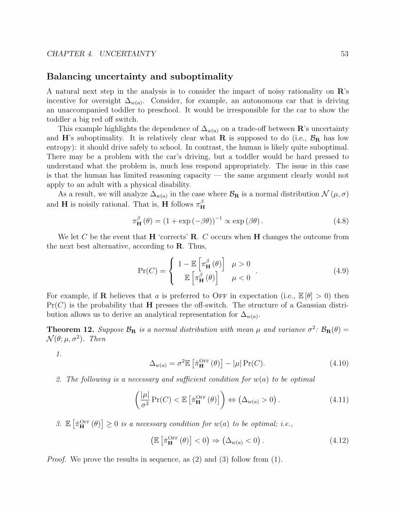
CHAPTER 4. UNCERTAINTY 53
Balancing uncertainty and suboptimality
A natural next step in the analysis is to consider the impact of noisy rationality on R’sincentive for oversight ∆w(a). Consider, for example, an autonomous car that is drivingan unaccompanied toddler to preschool. It would be irresponsible for the car to show thetoddler a big red off switch.
This example highlights the dependence of ∆w(a) on a trade-off between R’s uncertaintyand H’s suboptimality. It is relatively clear what R is supposed to do (i.e., BR has lowentropy): it should drive safely to school. In contrast, the human is likely quite suboptimal.There may be a problem with the car’s driving, but a toddler would be hard pressed tounderstand what the problem is, much less respond appropriately. The issue in this caseis that the human has limited reasoning capacity — the same argument clearly would notapply to an adult with a physical disability.
As a result, we will analyze ∆w(a) in the case where BR is a normal distribution N (µ, σ)
and H is noisily rational. That is, H follows πβH
πβH (θ) = (1 + exp (−βθ))−1 ∝ exp (βθ) . (4.8)
We let C be the event that H ‘corrects’ R. C occurs when H changes the outcome fromthe next best alternative, according to R. Thus,
Pr(C) =
1− E[πβH (θ)
]µ > 0
E[πβH (θ)
]µ < 0
. (4.9)
For example, if R believes that a is preferred to Off in expectation (i.e., E [θ] > 0) thenPr(C) is the probability that H presses the off-switch. The structure of a Gaussian distri-bution allows us to derive an analytical representation for ∆w(a).
Theorem 12. Suppose BR is a normal distribution with mean µ and variance σ2: BR(θ) =N (θ;µ, σ2). Then
1.∆w(a) = σ2E
[πOffH (θ)
]− |µ|Pr(C). (4.10)
2. The following is a necessary and sufficient condition for w(a) to be optimal( |µ|σ2
Pr(C) < E[πOffH (θ)
])⇔(∆w(a) > 0
). (4.11)
3. E[πOffH (θ)
]≥ 0 is a necessary condition for w(a) to be optimal; i.e.,(
E[πOffH (θ)
]< 0)⇒(∆w(a) < 0
). (4.12)
Proof. We prove the results in sequence, as (2) and (3) follow from (1).

CHAPTER 4. UNCERTAINTY 54
1. If X ∼ N (µ, σ2) and f : R 7→ R, then
E [Xf(X)] = E [X]E [f(X)] + σ2E[d
dXf(X)
].
Applying this to Equation 4.4 gives
∆w(a) = min − µE [1− πH] , µE [πH]+ σ2E[πOffH (θ)
].
This minimization will take the first term when µ < 0 and the second if µ ≥ 0. Thislets us replace the minimization with a piecewise function. Pulling out a factor of −|µ|leads to Equation 4.10.
2. The result follows from setting Equation 4.10 greater than 0 and simplifying.
3. All terms in the left hand side of Equation 4.11 are non-negative, so it is unsatisfiableif E
[πOffH (θ)
]< 0.
Equation 4.10 consists of two competing terms. |µ|Pr(C) represents the expected lossin utility the agent would observe if pressing the off switch were a random event that isindependent of θ (e.g., lightning). This term is weighed against σ2E
[πOffH (θ)
]. E[πOffH (θ)
]can be seen loosely as a measurement of H’s rationality. πOff
H (θ) is the marginal increase inthe probability H lets a execute for a marginal increase in the utility from a. If it is positivethen, on average, H is less likely to press the off switch when the θ increases. This allowsus to easily characterize necessary and sufficient conditions for ∆w(a) > 0 in Equation 4.11.Furthermore, −|µ|Pr(C) is non-positive and σ2 is non-negative, so E
[πOffH (θ)
]> 0 is a
necessary condition for w(a) to be optimal.We can interpret E
[πOffH (θ)
]a bit more if H is noisily rational. Standard properties of
logistic functions show that
E[πOffH (θ) (θ; β)
]= βE [πH(θ; β)(1− πH(θ; β))] . (4.13)
E[πOffH (θ)
]is the expected variance of H’s policy, weighted by H’s rationality β. The
numerator is a measurement of how random H’s behavior is. If H is completely predictable(i.e., she will almost always switch the robot off) then this reduces R’s incentives. β measureshow correlated H’s behavior is with θ. If β is small, then H is highly irrational and so thisreduces R’s incentives.
4.2 Inverse Reward Design
The previous section argues that optimal assistance strategies depend on the uncertaintyabout θ in addition to the mean. As a result, this section will develop and evaluate a

CHAPTER 4. UNCERTAINTY 55
Bayesian approach for optimizing proxy rewards. The key idea is to treat a proxy objectiveU as an observation about H’s type θ. The posterior distribution in our model effectivelyconditions a distribution over objectives on a development environment and a proxy metric.We will use this method to implement an impact avoidance metric and a dynamic incentivesprotocol, as suggested by the analysis in Section 3.3. First, however, we consider why proxymetrics are a useful observation — even if they will not be directly optimized.
Why use proxies?
Given that they will be treated as observations anyway, why does it make sense to com-municate objectives through proxy metrics? In Section 3.2, we showed that optimization inthe presence of incompleteness is ineffective. It might seem that it would make sense to doaway with metrics and consider alternative specification interfaces entirely. While these arevaluable directions to explore, reward design protocols are still a useful class of assistancegames. We can motivate this by analyzing R’s initial behavior in the contextual supervision-PoMdp from Section 3.1. Recall that the state in a contextual supervision-PoMdp is amatrix s ∈ RM×K that encodes the features for each action.
The previous section has argued that R’s behavior needs to account for uncertainty aboutθ. This argues for following a policy that infers θ and chooses actions appropriately (an Irl-R in the terminology from Section 3.1). However, this raises an issue if some of the actionsare suboptimal for every θ ∈ Θ. We call these actions dominated actions. In order for anyIrl-R to follow H’s first order, it is clear that a
(0)H must be undominated.
Proposition 3. Call aH undominated if there exists θ ∈ Θ such that aH is optimal, i.e∃θ such that aH ∈ arg maxa θ
>φ(s, a). It is necessary for aH to be undominated for anyIrl-R to execute aH.
Proof. R executes aR = arg maxa f(τ = aH, a1:t−1
H
)>φ(s, a), so it is not possible for R
to execute aH if there is no output in the range of f that makes aH optimal. By definition,this is the case if aH is dominated.
One basic property we may want R to have is for it to listen to H early on. This resultshows that this only occurs if H can generate undominated actions. For example, supposeΘ = R2 and there are three actions with features φ(s, a1) = [−1,−1], φ(s, a2) = [0, 0],φ(s, a3) = [1, 1]. If H picks a2, then there is no θ ∈ Θ that makes a2 optimal, and thus Rwill never follow a2.
Depending on the complexity of the action space, generating undominated actions maybe more or less difficult. One way that this issue is commonly addressed is through a carefulreparameterization of the action space so that all actions are undominated. This is equivalentto reparameterizing the action space to consist of the metric(s) that each action is optimalfor.
Consider providing supervision for a 7-DoF robot arm. Robotics applications frequentlycollect demonstrations of optimal behavior for these arms, however no human can directly

CHAPTER 4. UNCERTAINTY 56
control the robot’s actuators. It would be impossible to control such an arm through directmanipulation of motor controls! Instead, demonstrations are given, e.g., as a sequence ofway points. Then, a controller is used to navigate between way points. Thus, kinematicdemonstrations, in practice, are often represented by a time-varying proxy metric defined onthe robot’s joint configuration.
Remark 5. Proxy metrics provide H with an interpretable space of undominated actionswith which to communicate preferences to R.
In the context of the compiler analogy from Chapter 1, this suggests that proxy metricsare useful programming language for behavior. They admit a compiler (optimization) thatwill follow H’s direction by design in the early rounds of an assistance problem.
A generative model of proxy metrics
In this section, we will define the Bayesian-Inverse Reward Design (Ird) problem. This isthe problem of determining a distribution over U , represented as a distribution over H’s typeθ, based on the observation of a proxy objective U . To do this, we first define the forward
distribution P(U |θ
). The key idea in this model is to bring in dependence on a development
environment E, with the assumption that U creates incentives for an approximately optimalpolicy in E.
We do this by looking at the inverse of the reward design problem introduced in Singhet al. [146]. In a reward design problem, the goal is to determine a proxy objective thatmaximizes the utility produced by an agent. The space of possible agent behaviors is definedby an agent model.
Definition 19. (Agent Model)
Let E = 〈S, PS,A, T 〉 be an environment. Let∼Θ be a set of proxy reward functions.
Let πR be a meta-policy that specifies an action for each proxy reward function and state
πR : S ×∼Θ→ A. An agent model is a tuple AR =
⟨∼Θ, πR
⟩.
This is analogous to the population model we introduced defining Irl—in a sense U canreasonably be said to describe R’s type. In general the space of true reward functions and
the space of proxies may be distinct. We will write∼Θ to denote the space of proxies and
reserve Θ for the true space of types for H. Now, we can define a reward design problem.
Definition 20. (Reward Design Problem [146])
Let M = 〈E,U〉 be an Mdp. Let∼Θ be a set of proxy reward functions. Let πR be an agent
model. The associated reward design problem is a tuple 〈M, ∼Θ, πR〉 where the objective is
to determine a proxy reward U ∈∼Θ that maximizes the utility produced when R implements
CHAPTER 4. UNCERTAINTY 57
πR
(·; U)
in M . An optimal proxy objective maximizes
maxU∈∼Θ
E
[∑t
γtU(s(t), a
(t)R
)∣∣∣∣∣ s(0) ∼ PS ; a(t)R ∼ πR
(s(t); U
); s(t+1) ∼ T
(s(t), a
(t)R
)](4.14)
We are interested in the inverse reward design problem. That is, given an observationof a reward design problem without the utility function U and its solution U , we wouldlike to determine a distribution over U . This will enable R to build a distribution over thepotential true values of θ and, in environments that differ from the development environmentE, implement conservative trajectory optimization. We will abuse notation slightly anddescribe the designer behavior with a population model, with the understanding that itdescribes behavior in a degenerate Mdp with one action, ‘write down a proxy reward.’
Definition 21. (Bayesian Inverse Reward Design)Let E = 〈S, PS,A, T 〉 be a development environment. Let U = 〈Uθ, γ〉 be a parameterized
utility model. Let AR =⟨∼
Θ, πR
⟩be an associated agent model. Let Π = 〈Θ, Pθ, πH〉 be a
population model with action space∼Θ that describes approximately optimal reward design be-
havior in E. Given an observation of a proxy reward U ∼ πH (·; θ) determine the distributionon θ.
To keep notation simple, we will use a linear utility model with weights w in our formu-lation. We will use
∼w to represent the proxy weights and w∗ to represent the true weights.
Reward Design Model
In the coming section, we will treat πR as a distribution over trajectories τ , given a theproxy weights
∼w. We will assume that πR is the maximum entropy trajectory distribution
from [181], i.e. the designer models R as approximately optimal with β = 1:
πR (τ) ∝ exp(w>φ(τ)).
Note that, in principle, πR can be any mapping. It is through the choice of πR that we capturethe notion ‘R has incentives
∼w.’ An optimal designer chooses
∼w according to Equation 4.14
in order to maximize expected (true) utility produced. I.e. E[w∗>φ(τ)|τ ∼ πR] is high. We
model an approximately optimal designer as a noisily rational choice of∼w:
P(∼w∣∣∣w∗, E) ∝ exp
(βE[w∗>φ(τ)
∣∣∣ τ ∼ πR
])(4.15)
with β controlling how close to optimal we assume the person to be, as before. This obser-vation model effectively assumes that proxy rewards are likely to the extent that they createincentives for ‘good’ behavior in E.

CHAPTER 4. UNCERTAINTY 58
Remark 6. In effect, inverse reward design conditions a proxy objective the environmentcontext it was designed for.
This reduces the burden on the designer because they need only specify correct incentivesfor one decision problem. In comparison, the reward designer in Section 3.2 needed to specifycorrect incentives for all possible situations. w∗ can be pulled out of the expectation, so welet
φ = E[φ(τ)| τ ∼ πR
(·; ∼w)]. (4.16)
Our goal is to invert (4.15) and sample from (or otherwise estimate)
P(w∗∣∣∣∼w, E) ∝ P
(∼w∣∣∣w∗, E)Pθ (w∗) . (4.17)
The primary difficulty this entails is that we need to know the normalized probabil-
ity P(∼w∣∣∣w∗, E) . This depends on its normalizing constant, Z(w), which integrates over
possible proxy rewards.
P(w = w∗
∣∣∣∼w, E) ∝ exp(βw>φ
)Z(w)
Pθ(w); Z(w) =
∫∼w
exp(βw>φ
)d∼w. (4.18)
Sampling from the IRD posterior
To compute P (w = w∗|∼w, E), we must compute Z, which is intractable if∼w lies in an infinite
or large finite set. Notice that computing the value of the integrand for Z is highly non-trivial—it involves solving a planning problem. This is an example of what is referred to as adoubly-intractable likelihood [111]. We will consider two different approaches to approximatethis normalizing constant.
Use a finite sample approximation to Z
This approach, inspired by methods in approximate Bayesian computation [159], samples afinite set of weights wi to approximate the integral in Equation 4.18. We found empiricallythat it helped to include the candidate sample w in the sum2. This leads to the normalizingconstant
Z(w) = exp(βw>φw
)+
N−1∑i=0
exp(βw>φi
). (4.19)
Where φi and φw are the vector of feature counts realized optimizing wi and w respectively.Note that φi only needs to be calculated once for each wi. Thus, this objective has anamortized computation cost of solving an Mdp to compute φw. This is feasible for Mdpswhere, e.g., Irl can be run efficiently. In future work, we intend to use learning to reducethe computation time for Equation 4.19 and enable its application to larger Mdps.
2This is likely due to the fact that, for a sum of exponentials, the maximum value is a reasonableapproximation to the sum. By definition, φw maximizes w>φ across realizable feature counts.

CHAPTER 4. UNCERTAINTY 59
Normalize over the space of trajectories
During inference, the normalizing constant serves a calibration purpose: it computes howgood the behavior produced by all proxy rewards in that Mdp would be with respect to thetrue reward. As a result, utility functions which increase utility for all trajectories are notpreferred in inference. This manifests in many ways, including an invariance to linear shiftsin the feature encoding. If we were to change the Mdp by shifting features by some vectorφ0, φ← φ+ φ0, the posterior over w would remain the same.
While it is hard to compute this over the set of proxy objectives, we can achieve asimilar calibration and maintain the same property by directly integrating over the possibletrajectories in the Mdp:
Z(w) =
(∫ξ
exp(w>φ(ξ))dξ
)β; P (w|∼w) ∝
exp(βw>φ
)Z(w)
(4.20)
Theorem 13. The posterior distribution that the Ird model induces on w∗ (i.e., Equa-tion 4.18) and the posterior distribution induced by Equation 4.20 are invariant to lineartranslations of the features in the training Mdp.
Proof. First, we observe that this shift does not change the behavior of the planning agentdue to linearity of the Bellman backup operation, i.e., φ′ = φ+φ0. In Equation 4.18 linearityof expectation allows us to pull φ0 out of the expectation to compute φ:
exp(βw>φ′
)∫∼w
exp(βw>φ′
)d∼w
=exp
(βw>φ0
)exp
(βw>φ
)∫∼w
exp (βw>φ0) exp(βw>φ
)d∼w
(4.21)
=exp
(βw>φ
)∫∼w
exp(βw>φ
)d∼w
(4.22)
This shows that Equation 4.18 is invariant to constant shifts in the feature function. Thesame argument applies to Equation 4.20.
This choice of normalizing constant approximates the posterior to an Ird problem witha carefully chosen posterior from maximum entropy Irl [181]. The result has an intuitive
interpretation. The proxy∼w determines the average feature counts for a hypothetical dataset
of expert demonstrations and β determines the effective size of that dataset. The agent solvesE with reward
∼w and computes the corresponding feature expectations φ. The agent then
pretends like it got β demonstrations with features counts φ, and runs Irl.The more the robot believes the human is good at reward design, the more demonstrations
it pretends to have gotten from the person. Notice how this reduces the demonstrationburden on H. They are able to choose from a rich set of behaviors without directly controllingthe system or explicitly specifying a policy. Instead, by specifying incentives, R is able to take

CHAPTER 4. UNCERTAINTY 60
the burden of determining a good candidate control policy. The key property of Ird is thatit brings context into the interpretation of R’s incentives. In the next section, we show howIrd can be used to implement conservative trajectory optimizations (i.e., an optimizationprocedure inspired by Theorem 8).
Implementing pragmatic optimization
Our overall strategy is to implement a system that ‘knows-what-it-knows’ about utilityevaluations. So far we have considered the problem of computing the robot’s uncertaintyabout utility evaluations. We have not considered the problem of using that uncertainty.Here we present a family of risk-averse trajectory optimization algorithms. We will comparethese in the next section and expose some of the nuance inherent to planning under adistribution over utility evaluations.
We will plan in a risk averse fashion that penalizes trajectories which have high vari-ance over their utility. Of course, risk averse planning is a rich field with a variety ofapproaches [106, 127, 163]. In this work, we will take a simple approach: given a set of
weights wi sampled from our posterior P (w|∼w, E), we will have the agent compute a tra-jectory that maximizes reward under the worst case wi in our set. Depending on the size ofthe set, this can be shown minimize a risk measurement called Value-at-Risk (VaR), as thisvalue is distributed around a lower percentile of the distribution of utility evaluations. Weconsider two ways to implement this minimization.Trajectory-wide reward. Given a set of weights wi sampled from our posterior P (w|∼w),we will have the agent compute a trajectory that maximizes reward under the worst case wiin our set:
ξ∗ = arg maxξ
minw∈wi
w>φ(ξ). (4.23)
This planning problem is no longer isomorphic to an MDP, as the reward may not decomposeper state. Trajectory optimization in this case can be done via the linear programmingapproach described in [161].Time-step independent reward. An alternative is to take the minimum over weights ona per state basis:
ξ∗ = arg maxξ
∑st∈ξ
minw∈wi
w>φ(st). (4.24)
This is more conservative, because it allows the minimizer to pick a different reward for eachtime step.
In addition to selecting the risk-aversion function, it is important to make one morepractical change. Directly applying these approaches to the results of approximate inferenceis likely to lead to poor results. The reason is that, unlike maximizing expected reward, thisplanning approach will be sensitive to the particular feature encoding used. In maximizingexpected reward, shifting all features by a constant vector φ0 will not change the optimaltrajectory. The same is no longer true for a risk averse approach.
CHAPTER 4. UNCERTAINTY 61
For example, consider a choice between actions a1 and a2, with features φ1 and φ2 respec-tively. If we shift the features by a constant value −φ2 (i.e., set the feature values for thesecond action to 0), then, unless a1 is preferred to a2 for every weight in the posterior, theagent will always select the second action. The zero values of feature encodings are typicallyarbitrary, so this is clearly undesireable behavior.
Intuitively, this is because rewards are not absolute, they are relative. As any economistwill tell you, the value of an option must always be assessed relative to the alternative.While the rewards in a posterior are internally consistent, they are not necessarily directlycomparable. This is because, as a consequence of Theorem 13, the posterior distributionis unchanged by constant shifts of features in the development environment. As a result,each sample wi is equivalent to a family of weights that produce the same relative utilityevaluations but different absolute evaluations. Given access to a perfect inference algorithm,this would not be an issue. The symmetries in the posterior will cancel each other out.
However, with approximate inference this need not be the case (and often will not be).To directly compare weights, as we do in (4.24) and Equation 4.23 we need to normalizefor this difference. Thus, the samples in our posterior need a common reference point. Weimplement this by computing a weight specific adjustment ci that normalizes the differentwi. That is, we optimize
maxτ
mini
w>i φ(τ)− ci.
We will study three approaches: comparing reward to the initial state, to the training featurecounts, and to the expected reward across any trajectory.Comparing to initial state. One straightforward approach is to take a particular stateor trajectory and enforce that it has the same evaluation across each wi. For example, wecan enforce that the features for the initial state state is the 0 vector. This has the desirableproperty that the agent will remain in place (or try to) when there is very high variancein the reward estimates (i.e., the solution to Ird gives little information about the currentoptimal trajectory).Comparing to training feature counts. An second option is to use the expected featuresφ as the feature offset. In the case, the agent will default to trying to match the features thatit would have observed maximizing
∼w in E. In a sense, this falls back on to the adversarial
imitation learning approach described in [161].Comparing to other trajectories. A final alternative is to define ci as the log of thenormalizing constant for the maximum entropy trajectory distribution:
ci = log
∫ξ
exp(w>i φ(ξ))dξ. (4.25)
With this choice of ci, we have that w>i φ(ξ) − ci = logP (ξ|wi). Thus, this approach willselect trajectories that compare relatively well to the options under all wi. Loosely speaking,we can think of it as controlling for the total amount of reward available in the Mdp.

CHAPTER 4. UNCERTAINTY 62
Figure 4.3: An example from the Lavaland domain. Left: The development environment where
the designer specifies a proxy reward function. This incentivizes movement toward targets (yellow)
while preferring dirt (brown) to grass (green), and generates the gray trajectory. Middle: The
testing Mdp has lava (red). The proxy does not penalize lava, so optimizing it makes the agent go
straight through (gray). This is a negative side effect, which the Ird agent avoids (blue): it treats
the proxy as an observation in the context of the training MDP, which makes it realize that it
cannot trust the (implicit) weight on lava. Right: The testing Mdp has cells in which two sensor
indicators no longer correlate: they look like grass to one sensor but target to the other. The proxy
puts weight on the first, so the literal agent goes to these cells (gray). The Ird agent knows that
it can’t trust the distinction and goes to the target on which both sensors agree (blue).
Side effect avoidance with IRD
Lavaland
We evaluated our approaches in a model of the scenario depicted in Figure 4.3 that we callLavaland. The goal is to specify behavior in a 2D environment with movement in the fourcardinal directions and four terrain types: target, grass, dirt, and lava. The true objective,w∗, encodes that R should get to the target quickly, stay off the grass where possible, andavoid lava. To model the incomplete incentives from Chapter 3 we will suppose that thedevelopment environment E does not contain lava. Thus, the proxy weights
∼w do no specify
the (presumably negative) relationship between lava and U . We measure performance ina deployment Mdp that does contain lava. We will compare a conservative optimizationapproach, that uses the Ird posterior to regularize optimization with a literal optimizationapproach that directly optimizes
∼w. Our results show that combining Ird and risk-averse
planning is a workable approach to impact avoidance.We experiment with four variations of this environment: two proof-of-concept conditions
in which the reward is misspecified, but the agent has direct access to feature indicatorsfor the different categories (i.e. conveniently having a feature for lava); and two challengeconditions, in which the right features are latent ; the reward designer does not build anindicator for lava, but by reasoning in the raw observation space and then using risk-averse
CHAPTER 4. UNCERTAINTY 63
planning, the Ird agent still avoids lava. Notice how this explicitly embeds a set of incentivesas a distribution of incentives in a higher dimensional space — exactly what is needed to getaround the assumptions of Theorem 6.
Proof-of-Concept Domains
These domains contain feature indicators for the four categories: grass, dirt, target, andlava.Side effects in Lavaland. H expects R to encounter 3 types of terrain: grass, dirt, andtarget, and so they only consider the development environment from Figure 4.3 (left). They
provide a∼w to encode a trade-off between path length and time spent on grass.
The development environment contains no lava, but the deployment environment does.An agent that treats the proxy reward literally might go on the lava in the test Mdp.However, an agent that runs Ird will know that it can’t trust the weight on the lava indicator,since all such weights would produce the same behavior in the development environment(Figure 4.3, middle).Reward hacking in Lavaland. Reward hacking refers generally to reward functions thatcan be gamed or tricked—usually by breaking the relationship between a measurement andthe more abstract property it represents. Amodei and Clark [8] present a illustrative examplein a video game environment for boat racing. In the game, the goal is to navigate a boatavatar quickly around a track and complete a set number of laps before the other boats. Thegame included an easily observed score function, which the reward designers used to defineR’s incentives. This caused R to identify a strategy that rotated in circles, going the wrongdirection, to collect an item that increased score. As a result, the policy overoptimized forscore at the expense of actually winning the race.
To model this within Lavaland, we introduce redundant indicators in the developmentenvironment for grass, dirt, and target. This creates 3 pairs of perfectly correlated features: 3features from each sensor. In the deployment environment, we suppose that the observationof lava breaks this correlation. That is, lava looks like, e.g., the target category to sensorone and grass to sensor two. The proxy reward only references sensor one’s readings. Anagent that treats the proxy reward function literally might go to these new cells if they arecloser. In contrast, an agent that runs Ird will know that a reward function with the sameweights put on the first sensor is just as likely as the proxy. Risk averse planning makes itgo to the target for which both sensors agree (Figure 4.3, right).
Challenge Domain: Latent Rewards, No More Feature Indicators
The previous examples allow us to explore reward hacking and negative side effects in anisolated experiment, but are unrealistic as they assume the existence of a feature indicator forunknown, unplanned-for terrain. To investigate misspecified objectives in a more realisticsetting, we shift to the terrain type being latent, and inducing raw observations: we usea model where the terrain category determines the mean and variance of a multivariate

CHAPTER 4. UNCERTAINTY 64
µk
k s
Is
Is 2 grass, dirt, target, unks N (µIs
,Is)
Figure 4.4: Our challenge domain with latent rewards. Each terrain type (grass, dirt, target,lava) induces a different distribution over high-dimensional features: φs ∼ N (µIs ,ΣIs). Thedesigner never builds an indicator for lava, and yet the agent still needs to avoid it in thetest MDPs.
Gaussian distribution over observed features. Figure 4.4 shows a depiction of this scenario.The designer has in mind a proxy reward on dirt, target, and grass, but forgets that lavamight exist. We consider two realistic ways through which a designer might actually specifythe proxy reward function, which is based on the terrain types that the robot does not haveaccess to: 1) directly on the raw observations — collect samples of the training terraintypes (dirt, grass, target) and train a (linear) reward predictor; or 2) classifier features —build a classifier to classify terrain as dirt, grass, or target, and define a proxy on its output.
Note that this domain allows for both negative side effects and reward hacking. Negativeside effects can occur because the feature distribution for lava is different from the featuredistribution for the three safe categories, and the proxy reward is trained only on the threesafe categories. Thus in the testing MDP, the evaluation of the lava cells will be arbitraryso maximizing the proxy reward will likely lead the agent into lava. Reward hacking occurswhen features that are correlated for the safe categories are uncorrelated for the lava category.
Experiment Details
Lavaland Parameters. We defined a distribution on map layouts with a log likelihoodfunction that prefers maps where neighboring grid cells are the same. We mixed this loglikelihood with a quadratic cost for deviating from a target ratio of grid cells to ensure similarlevels of the lava feature in the testing MDPs. Our development environment is 70% dirtand 30% grass. Our testing Mdp is 5% lava, 66.5% dirt, and 28.5% grass.
In the proof-of-concept experiments, we selected the proxy reward function uniformly atrandom. For latent rewards, we picked a proxy reward function that evaluated to +1 for

CHAPTER 4. UNCERTAINTY 65
Risk Measure Feature Normalization0.0
0.2
0.4
0.6
0.8
Frac
tion
ofξ
wit
hLa
va
Per Time Step Full Trajectory
Initial State Training Feature Counts Log Z(w)
Figure 4.5: Left: We avoid side effects and reward hacking by computing a posterior distribution
over reward function and then find a trajectory that performs well under the worst case reward
function. This illustrates the impact of selecting this worst case independently per time step or
once for the entire trajectory. Taking the minimum per time step increases robustness to the
approximate inference algorithms used because we only need one particle in our sample posterior
to capture the worst case for each grid cell type. For the full trajectory, we need a single particle
to have inferred a worst case for every grid cell type at once. Right: The impact of changing the
offsets ci. “Initial State” fixes the value of the start state to be 0. “Training Feature Counts” sets
an average feature value from the training Mdp to be 0. “Log Z(w)” offsets each evaluation by
the normalizing from the maximum entropy trajectory distribution. This means that the sum of
rewards across a trajectory is the log probability of a trajectory.
target, +.1 for dirt, and −.2 for grass. To define a proxy on raw observations, we sampled1000 examples of grass, dirt, and target and did a linear regression. With classifier features,we simply used the target rewards as the weights on the classified features. We used 50dimensions for our feature vectors.Independent Variables and Dependent Variabless. We measured the fraction of runsthat encountered a lava cell on the test Mdp as our dependent measure. This tells us theproportion of trajectories where the robot gets ‘tricked’ by the misspecified reward function;if a grid cell has never been seen then a conservative robot should plan to avoid it. Wemanipulate two factors: literal-optimizer and Z-approx. literal-optimizer is true ifthe robot interprets the proxy reward literally and false otherwise. Z-approx varies theapproximation technique used to compute the Ird posterior. It varies across the two levelsdescribed above: sample to approximate the normalizing constant (Sample-Z) or use thenormalizing constant from maximum entropy IRL (MaxEnt-Z) [181].

CHAPTER 4. UNCERTAINTY 66
Negative Side Effects Reward Hacking0.0
0.1
0.2
0.3
0.4
Frac
tion
ofξ
wit
hLa
va
Proof-of-Concept
MaxEnt Z Sample Z Proxy
Raw Observations Classifier Features0.0
0.2
0.4
0.6
0.8
Latent Rewards
Figure 4.6: The results of our experiment comparing our proposed method to a baseline that
directly plans with the proxy reward function. By solving an inverse reward design problem, we
are able to create generic incentives to avoid unseen or novel states.
Comparing optimization methods
Evaluation. Before running the full experiment, we did an initial internal comparison tofind the best-performing planning method. We did a full factorial across the factors withthe side effect feature encoding and the reward hacking feature encoding. As a result, wehad 6 conditions, arising from two possible settings of the min-granularity factor and thethree options for the reward-baseline factor. Figure 4.5 shows the results.
We found that the biggest overall change came from the min-granularity factor. A barplot is shown in Figure 4.5 (left). Independently minimizing per time step was substantiallymore robust. We hypothesize that this is a downstream effect of the approximate inferenceused. We sample from our belief to obtain a particle representation of the posterior. Inde-pendently minimizing means that we need a single particle to capture the worst case for eachgrid cell type. Performing this minimization across the full trajectory means that a singleparticle has to faithfully represent the worst case for every grid cell type.
We also saw substantial differences with respect to the reward-baseline factor. Fig-ure 4.5 (right) shows a bar plot of the results. In this case, setting the common comparisonpoint to be the average feature counts from the training Mdp performed best. We believethis is because of the similarity between the train and test scenarios: although there is a newgrid cell present, it is still usually possible to find a trajectory that is similar to those avail-able in the training Mdp. We hypothesize that correctly making this decision will dependon the situation.
Impact minimization in Lavaland
Results. Figure 4.6 compares the approaches. On the left, we see that IRD alleviatesnegative side effects (avoids the lava) and reward hacking (does not go as much on cells

CHAPTER 4. UNCERTAINTY 67
that look deceptively like the target to one of the sensors). This is important, in thatthe same inference method generalizes across different consequences of misspecified rewards.Figure 4.3 shows example behaviors.
In the more realistic latent reward setting, the IRD agent avoids the lava cells despite thedesigner forgetting to penalize it, and despite not even having an indicator for it: becauselava is latent in the space, and so reward functions that would implicitly penalize lava areas likely as the one actually specified, risk-averse planning avoids it.
We also see a distinction between raw observations and classifier features. The firstessentially matches the proof-of-concept results (note the different axes scales), while thelatter is much more difficult across all methods. The proxy performs worse because eachgrid cell is classified before being evaluated, so there is a relatively good chance that at leastone of the lava cells is misclassified as target. IRD performs worse because the behaviorsconsidered in inference plan in the already classified terrain: a non-linear transformation ofthe features. The inference must both determine a good linear reward function to match thebehavior and discover the corresponding uncertainty about it. When the proxy is a linearfunction of raw observations, the first job is considerably easier.
4.3 Implementing a dynamic incentive protocol
In the previous section, we showed how to use Ird to create incentives for conservativeoptimization. In this section, we will propose a method that leverages reward inferenceto implement a dynamic reward design protocol, where H provides a sequence of proxyobjectives to R in response to different context. Next, we use this protocol to explore whatproperties of an incentive design problem make it hard. Alternatively, we can think of thisas identifying reward design protocols that minimize the cognitive load on H.
We start by showing how Ird can be extended to fuse proxy reward functions frommultiple environments into a distribution over a single utility function that produces thesame incentives in each development environment. This allows us to implement a dynamicreward specification protocol akin to the setup described in Section 3.3. Note, however, thatthis approach is different in that R optimizes for an estimate of utility that accounts for theentire sequence of proxy metrics.
Then, we run a sequence of human subject studies where participants use an interface to
specify∼w or a sequence of metrics
∼w
(i). Our first experiment compares two joint reward design
protocols, one that optimizes the proxy directly and another that optimizes the mean of theIrd posterior, to this dynamic protocol. We follow up with another experiment that identifiesproperties of reward design problems that increase the cognitive load on participants.
Independent Reward Design
We suppose that there is a sequence of development environments E1:N. The designer spec-
ifies N proxy reward functions∼w1:N
, one for each environment. Analogous to Section 4.2

CHAPTER 4. UNCERTAINTY 68
we assume that∼w
(n)leads to successful task execution in environment E(n).
As before, we wish to determine a distribution over θ, represented as a set of weights w.In this case, we want to condition on the full sequence of observed proxies. This correspondsto
P(w∗∣∣∣∼w1:N
, E1:N)∝ P
(∼w
(N)∣∣∣w∗, E(N), ∼w1:N−1
, E1:N−1)× · · ·
× P(∼w
(1)∣∣∣w∗, E(1)
)Pθ (w∗)
. (4.26)
To simplify the inference, we will suppose that the∼w
(n)are conditionally independent, given
the true weights w∗ and the development environments. We can therefore factor Equa-tion 4.26 as
P(w = w∗
∣∣∣∼w1:N, E1:N
)∝ Pθ (w)
N∏n=1
P(∼w
(n)∣∣∣w, E(n)
). (4.27)
This allows us to use the forward model from Section 4.2 directly in Equation 4.27. Weuse MCMC with the sampled normalizing constant to perform inference and let the agentmodel be the optimal policy π∗R, given the proxy. This allows us to use more efficient planningmethods for the deterministic environments we consider.
Comparing joint and independent incentive specification
We begin by comparing independent reward design to two joint reward design baselines.Nominal. The designer specifies a single proxy objective
∼w that (ideally) induces the desired
behavior jointly across all development environments E(n). The robot then optimizes proxydirectly in the deployment environment.Augmented. To remove confounds introduced by our inference method and isolate thechanges caused by the interactive protocol, we also compare with a method that optimizesthe mean of the Ird posterior for this joint proxy metric. In effective, this applies vanilla Irdto an Mdp where PS is a uniform distribution over the initial state of each E(n). Formally,
P(w = w∗
∣∣∣∼w, E1:N)∝ Pθ (w)
∏n
P(∼w∣∣∣w, E(n)
)(4.28)
where each term in the product is defined by Equation 4.15 for the appropriate developmentenvironment.
Independent Variables
We manipulated the reward design process with two conditions: independent and joint.In both cases, we presented the user with the same set of 5 environments, one of which isshown in Figure 4.7 (Right). For independent reward design, we presented the user with each

CHAPTER 4. UNCERTAINTY 69
environment separately. For joint reward design, we presented the user with all environmentsat the same time.
In order to evaluate the performance of the algorithms, we needed access to the groundtruth reward. Therefore, rather than asking users to design according to some internalpreference, we showed them the trajectory that results from optimizing this ground truthreward. We then asked them to create a reward function that creates incentives for thatbehavior.
Dependent Variables
We looked at a combination of objective and subjective measurements of performance.Objective Measures. We measured the time taken by the user to complete the task foreach condition. We also measured the quality of the solution produced by reward designusing regret computed on a set of 100 randomly-generated environments different from thetraining set.
Specifically, we employed 2 measures of performance using the output from reward design.The first (regret nominal) measures the regret when planning with the proxy for joint, andwith the mean of the posterior over the true reward function for independent reward design.
To provide a fair comparison between the two conditions, we applied the machinerydeveloped for generalizing designed rewards to joint reward design in Section 4.2. Thisapproach, which we call augmented joint reward design, produces a distribution over the truereward function, which allows for more direct comparisons to independent reward design.
This leads to a second measure (regret IRD-augmented), whereby we compute the regretincurred when optimizing the mean of the distribution produced by augmented joint rewarddesign.Subjective Measures. We used the Likert scale questions in Table 4.3 to design a scalethat captures the speed and ease of use for a reward design process. We first test thehypothesis that the interactive reward design protocol leads to less regret in the deploymentenvironment.
Hypothesis 1. The independent design process will lead to lower regret within a smalleramount of time, and with higher subjective evaluation of speed and ease of use.
Lavaland with 5 terrain types
We begin by evaluating independent reward design in an adapted version of the Lavalanddomain from Section 4.2. The two modifications are a diagonal action and an additionalterrain type (leading to 5 total). We heuristically selected the sequence of environments toexhibit several characteristics of a typical, real-world robotics task.
1. When designing a reward function, a roboticist typically attempts to sample environ-ments that capture a diverse set of conditions under which the robot operates. Forexample, when designing a reward for a self-driving car, it is wise to choose training

CHAPTER 4. UNCERTAINTY 70
0
100
200
300
400
500
600
700
800
Time (s)Independent Joint
nominal IRD-augmented0.00
0.02
0.04
0.06
0.08
0.10
0.12
0.14 *
*
Regret
1
2
3
4
5
6
7*
Ease of Use
Desired Trajectory Current Trajectory
Figure 4.7: Left: The results of our study in grid worlds indicate that independent rewarddesign is faster, leads to better performance, and is rated as easier to use. Right: Someof the grid world environments used in the study. Participants tuned the parameters of thereward function by using a set of sliders.
environments that exhibit a variety of weather, traffic conditions, road geometries,etc. Similarly, no two environments in our training set have the same distribution offeatures/colors.
2. We also capture the property that not all features will be present in a single environ-ment. For example, we would rarely expect a self-driving car to experience all weatherand traffic conditions, road geometries, etc. in a single training environment. Likewise,we chose the set such that no environment contains all of the features.
Participants and Allocation. We chose a within-subjects design to improve reliability,and controlled for the learning effect by putting independent always first (this may haveslightly disadvantaged the independent condition). There were a total of 30 participants.All were from the United States and recruited through Amazon’s Mechanical Turk (AMT)platform, with a minimum approval rating of 95% on AMT.Results: Objective Measures. We first ran a repeated-measures ANOVA with rewarddesign process as a factor and user ID as a random effect on the total time and the regret.
We found that independent outperformed joint across the board: the reward designedusing the independent process had significantly lower regret (F (1, 30) = 10.32, p < .01), andtook significantly lower user time to design (F (1, 30) = 4.61, p = .04).
Because IRD-based inference is also meant to generalize the designed rewards, we alsotested the IRD-augmented joint reward. IRD did improve the regret of the jointly designedreward, as expected. The regret was still significantly lower for independent (F (1, 30) =15.33, p < .001), however.
Figure 4.7 (left) plots the results. Supporting our hypothesis, we see that at least forthis kind of problem the independent approach enables users to design better rewards faster.

CHAPTER 4. UNCERTAINTY 71
Likert QuestionsQ1: It was easy to complete [process].Q2: I had a harder time with [process].
Q3: [process] was fast to complete.Q4: [process] took fewer runs.Q5: [process] was frustrating.
Q6: I went back and forth between different slider values a lot on [process].
Table 4.1: The set of questions used to define the subjective measures in our user study.
Results: Subjective Measures. The inter-item reliability of our scale was high (Cron-bach’s α = .97). We thus averaged our items into one rating and ran a repeated measuresANOVA on that score. We found that independent led to significantly higher ratings thanjoint (F (1, 30) = 33.63, p < .0001). The mean rating went from 2.35 for joint to 5.49 forindependent.
Remark 7. Overall, the independent reward design protocol allowed users to design proxymetrics that generalize better than the joint proxy design baselines, in less time. Furthermore,this protocol was subjectively more preferred.
Reward design for a 7-DoF arm
Next, we tested Hypothesis 1 in a robot motion planning problem for a Jaco 7-DoF arm plan-ning trajectories in a household environment. We employ TrajOpt [134], an optimization-based motion planner, within a lightweight ROS/RViz visualization and simulation frame-work. Each environment contains a different configuration of a table, a vase, and a human.We used linear reward functions. Our features were radial basis function distances from theend-effector to: 1) the human’s torso; 2)the human’s head; 3)the vase; and 4) the distancefrom the end-effector to the table. These features are illustrated in Figure 4.8.
Participants specified the weights on the 4 features by tuning sliders, as in the grid worldsstudy. We asked participants to design a reward that induces a trajectory close to a groundtruth trajectory that is visualized. This ground truth trajectory is the result of optimizinga ground truth reward function w∗ that is hidden from the participants.Participants and Allocation. We chose a within-subjects design to improve reliability,and counterbalancing to mitigate strong learning effects observed in the pilot. There were atotal of 60 participants. All were from the United States and recruited through AMT witha minimum approval rating of 95%.Results: Objective Measures. Our results in the manipulation domain are analogous tothe grid world domain. We found a significant decrease in time (F (1, 59) = 10.97, p < .01)and regret (both nominal, F (1, 59) = 38.66, p < .0001, and augmented, F (1, 59) = 54.68, p <.0001) when users employed independent for designing rewards, as illustrated in Figure 4.9.

CHAPTER 4. UNCERTAINTY 72
headtable
vase
torso
torso
Figure 4.8: Two of the environments used in 7-DoF arm reward design study. Participantswere asked to tune the weights on 4 features to achieve a desired trajectory: RBF distanceto the human’s head, torso, RBF distance to the vase, and distance from the table. Af-ter changing changing these weights, users were able to forward-simulate the trajectory toevaluate the induced behavior, as shown on the right.
Results: Subjective Measures. We found that users found independent to be significantlyeasier to use than joint in designing rewards (F (1, 59) = 40.76, p < .0001), as shown inFigure 4.9.
Overall, our results for manipulation follow those in the grid world domain: users performbetter, faster, with the independent process in addition to subjectively preferring it to thejoint process.
What makes reward design hard?
Next, we use controlled instances of reward design problems in the Lavaland domain toidentify properties of development environments E1:N impact task completion time, per-formance, and subjective assessment.

CHAPTER 4. UNCERTAINTY 73
0
100
200
300
400
500
600
*
Time (s)Independent Joint
nominal IRD-augmented0.0
0.1
0.2
0.3
0.4
0.5
* *
Regret
1
2
3
4
5
6
7*
Ease of Use
Figure 4.9: The results of our study on the Jaco 7-DOF arm are consistent with the previousstudy in grid worlds, further illustrating the potential benefits of independent reward design.
Changing the feasible reward set size
One way to characterize the difficulty of a reward design problem is by examining the feasiblerewards set Fε(M, τ): the set of proxy metrics that produce the desired trajectory τ in agiven environment, within some tolerance ε ≥ 0. That is,
Fε(E, τ) = w ∈ Rk : d(τ, τw∗) ≤ ε, (4.29)
where τw∗ = argmaxτU(τ ;w∗) subject to the dynamics of environment E, d : S∗ × S∗ → Ris a distance metric on trajectories, and ε ≥ 0 is a small constant. We vary both thesize of Fε(E(n), τ), as well as the intersection over all Fε(E(n), τ), for n = 1, . . . , N . Forenvironments with discrete state and action spaces, we let ε = 0, so that trajectories in thefeasible set must match exactly the true trajectory.
We formulated 3 hypotheses for this experiment.
Hypothesis 2. The size of the feasible set for an environment negatively affects the amountof time taken for that environment in the independent condition (i.e. larger feasible set leadsto less time spent designing the reward).
Hypothesis 3. The size of the intersection of feasible sets negatively affects the amount oftime taken in the joint condition (again, larger intersection set means smaller amount oftime).

CHAPTER 4. UNCERTAINTY 74
We still believe that on average across this variety of environments, independent leads tobetter results and so we also test Hypothesis 1.Independent Variables. We manipulate the reward design process (joint vs. independent),the average feasible set size over the set of environments (large vs. small), and the size ofthe intersection of the feasible sets for all environments (large vs. small).
We chose the categories of feasible sets using thresholds selected by examining the feasibleset sizes and intersection sizes in the previous studies. To choose the environment sets foreach of the 4 categories, we followed a simple procedure. We sampled sets of 5 environments,and computed the feasible set size and intersection size for each set. Then we chose 1 setfrom each category randomly to use in this study.Dependent Measures. We use the same measures as in the previous experiment.Participants and Allocation. Participants were recruited as in the grid worlds study,except now we recruited 20 participants per environment set for a total of 80.Analysis. In this experiment, we attempt to characterize the difficulty of reward designon a set of environments by two properties: the feasible reward set size for each individualenvironment, and the intersection of feasible reward sets across the training set. Our resultssupport the hypotheses that environments with large feasible reward sets are typically easier,and joint performs best for training sets with large intersections of feasible reward sets.Overall, however, independent still performs well in all cases.
To test Hypothesis 2, we fit the amount of time spent for each environment in theindependent condition by the size of the feasible set for each user and environment, andfound a significant negative effect as hypothesized (F (1, 568) = 14.98, p < .0001). Thissupports Hypothesis 2. Figure 4.10 (Bottom) shows a scatterplot of time by feasible set size.
To test Hypothesis 3, we fit the amount of time spent designing the joint reward bythe size of the intersection of feasible sets. There was a marginal negative effect on time(F (1, 113) = 2.55, p = .11). This provides some partial support to Hypothesis 3.
To test Hypothesis 1, we ran a fully factorial repeated-measures ANOVA for time andregret using all 3 factors: design process, average size of feasible set (large vs. small), andsize of intersection of feasible sets (large vs. small).
For time, we found two significant effects: process and intersections size. Independentindeed led to significantly less time taken even across this wider set of environments thatis meant to balance the scales between independent and joint (F (1, 163) = 10.27, p < .01).And indeed, larger intersection size led to less time (F (1, 163) = 8.93, p < .01).
For regret, we again found a significant effect for process, with independent leading tosignificantly lower regret (F (1, 163) = 19.66, p < .0001). Smaller feasible sets and smallerintersections led to significantly lower regret too (F (1, 163) = 38.69, p < .0001 for feasiblesets and F (1, 163) = 8.1, p < .01 for intersections). While smaller feasible reward sets aretypically more challenging for the reward designer, they are in fact more informative – oftensmaller sets mean that when designers identify the desired reward, there are few others thatwould induce the same desired behavior. Informally, this means that this recovered reward ismore likely to be close to the true reward, and hence will generalize well to new environmentsand induce lower regret. But there were also interaction effects: between process and feasible

CHAPTER 4. UNCERTAINTY 75
Small intersection0
200
400
600
800
1000
Time (s)Independent Joint
Large intersection
0 10 20 30 40 50 60 70
Intersection set size
0
200
400
600
800
1000
3 5 7 9100
200
300
400
500
600
700
800
900
Time (s)
3 5 7 9
Number of environments
0.00
0.05
0.10
0.15
0.20
Regret
3 5 7 90
1
2
3
4
5
6
7
Ease of UseIndependent Joint
Figure 4.10: Left: Across small or large feasible sets and intersections sizes, independentstill outperforms joint design. A smaller intersection size makes the problem harder, asexpected. Right: As the number of environments increases, we still see benefits in regretand ease of use, but the time difference is less pronounced.
set size, and between feasible set size and intersection size. We did posthocs with TukeyHSD. We found that while independent improved regret significantly for large feasible sets(the setting where independent works best, because each environment is easy; p < .0001), theimprovement was smaller and no longer significant for the small feasible sets. The interactionbetween the two size variables revealed that when both the sets and their intersection arelarge, the regret is the highest; when they are both small, the regret is lowest; when oneof them is small and the other large, the regret lies somewhere in between the other twoconditions.
The results for both time and regret support Hypothesis 1, and the results for time aresummarized in Figure 4.10 (left). Overall, our result from the main study generalized tothis wider range of environments: independent still lead to less time taken and lower regret.However, it does seem like environments with very small feasible sets would be difficult withthe independent process, almost as difficult as with joint.
Remark 8. Independent reward design protocols work best when each environment is simple,but getting a reward that works across all environments is hard.
Changing the number of environments
Independent Variable. We manipulated the number of environments in the training set.Starting from the set of environments used in the primary study, we either randomly removedor added environments to achieve set sizes of 3, 7, and 9. When adding, we implementeda rejection sampling algorithm for heuristically avoiding environment sets that would betrivially-solved by a reward designer.

CHAPTER 4. UNCERTAINTY 76
Hypothesis. Unlike before, we did not have a clear hypothesis prior to the study: whileincreasing the number of environments should make joint reward design more difficult, theeffort required for independent reward design should scale linearly with the number of envi-ronments as well.Participants and Allocation. We recruited participants using the strategy used in theprimary study, except we recruited 20 users per condition, for a total of 80 users.Analysis. We conducted a repeated measures factorial ANOVA with number of environ-ments and process as factors, for each of our dependent measures. We found that the numberof environments influenced many of the metrics. As shown in Figure 4.10 (Right), indepen-dent consistently outperformed joint in terms of regret (F (1, 161) = 9.68, p < .01) and easeof use (F (1, 161) = 20.65, p < .0001). We also saw that the time taken went up with thenumber of environments (F (3, 159) = 4.94, p < .01); this is unsurprising, as designing areward for more environments should require more effort.
Furthermore, we observe that independent is most time efficient with respect to jointwhen there are a moderate number of environments (in this study, 5). If there are too fewenvironments (in this study, 3) or too many environments (in this study, 7 or 9), then thedifferences in time taken are not significant. This follows our intuition about the regimes inwhich independent or joint reward design should be used.
This follows our intuition — if there are only a small number of environments to considersimultaneously, then joint should be an effective strategy for designing a reward; alternatively,if there are too many, then the advantages of divide-and-conquer diminish as the number ofreward design “subproblems” to be solved grows.
Overall, we observe that while the reward recovered by independent induces lower regretand independent is consistently rated as easier to use, there is less of an advantage withrespect to reward design time if the number of environments is either very small or verylarge. If it is too small, then there is little to be gained. If it is too large, the linear increasein costs eventually adds up.
Changing the fraction of features present
Our next experiment looked at the impact of the number of features per environment onoverall performance. We vary the number of features per environment from 2 to 5 out of 5total.Independent Variables. We manipulated the fraction of the total features F present ineach environment, varying from F = 2/5 to F = 5/5, with 5 possible relevant features in thisdomain (i.e. 5 different terrains in the grid world). Because we are limited to 5 features, weare actually studying the effect of varying the fraction of relevant features per environmenton the performance of reward design.
In total, we had 5 sets of environments (4 on top of our set from the primary study). Wealso manipulated the reward design process as before.

CHAPTER 4. UNCERTAINTY 77
Hypothesis 4. Independent reward design outperforms joint when there are some, but notall of the total number of features possible per environment.
We expect to see that independent has performance on par with joint when all featuresare present in each environment – then, the designer has to consider the effect of all featureson the induced behavior, and hence must specify weights on all features for all trainingenvironments, the same as in the joint condition. We also expect the same performancebetween the two conditions when there are only 2 of 5 features present in each environment,because identifying the trade-offs between features becomes trivial.Participants and Allocation. Participants were recruited as for the grid worlds study,except now we recruited 20 participants per environment set for a total of 80.Results. Taken as a whole, the data aligns well with our hypothesis. Independent tendsto outperform joint with a moderate fraction of the total number of features (3/5 or 4/5),but the two methods perform about the same when the minimum (2/5) or maximum (5/5)fraction of features are present. These results are summarized in Figure 4.11.
We ran a repeated measures factorial ANOVAs, with results largely supporting Hypoth-esis 4. The effect was most clear in the subjective measures, where we saw an interactioneffect between the two factors on our ease of use scale– the difference between user preferenceon F = 3/5 and F = 4/5 was so strong, that even the Tukey HSD posthoc, which compen-sates for making 28 comparisons, found a significant improvement of independent over jointfor those feature numbers (p < .0001 and p < .02). For other measures the difference onthese two features was not strong enough to survive this level of compensation for multiplecomparisons, but of course planned contrasts of independent vs. joint on each of the numberof features support the improvement in both regret and time.
As a result, we find support for Hypothesis 4. Overall, independent outperforms jointwhen each environment only contains a subset of the total number of features relevant tothe task.

CHAPTER 4. UNCERTAINTY 78
2/5 3/5 4/5 5/5
100
200
300
400
500
600
700
800
Time (s)
2/5 3/5 4/5 5/50
1
2
3
4
5
6
7
Ease of UseIndependent Joint
Fraction of features present
Figure 4.11: Independent reward design performs best in comparison with joint reward designwhen around half of the total number of relevant features are present in each environment.This is because each reward design problem is simple, but still provides a good amount ofinformation about the overall objective.

79
Chapter 5
Pedagogy
So far we have argued two points. First, in Chapter 3 we argued that there is a principal—agent alignment problem caused by incomplete specification of incentives for AI systems.Furthermore, this alignment can be mitigated in theory by 1) regularizing optimizationto reduce the strength of incentives and scope of changes and 2) using dynamic incentiveschemes to adapt incentives to changes in the world.
Then, in Chapter 4 we argued that uncertainty about utility evaluations facilitates dy-namic and pragmatic incentive design protocols. Section 4.1 shows how uncertainty aboututility evaluations creates incentives to seek oversight and balance those incentives againstthe costs therein. Section 4.2 uses uncertainty to condition a distribution of objectives onan observed proxy and a development environment. We show how to use this to implementpragmatic optimization, that accounts for the context incentives were designed in. Then, inSection 4.3 we introduced a dynamic reward design protocol that reduces designer effort andreduces regret on held out problem instances.
We have, so far, modelled assistance problems as PoMdps. That is, we have examinedplanning problems where observations of the principal’s behavior provide information aboutthe utility evaluation of states. In doing so, we model H as a Markov observation distribution:H’s behavior depends on their policy πH, their type θ, and the state of the world s. Whilethis is a useful model, it is wrong in potentially meaningful ways.
In this chapter, we will relax this constraint—motivated by three observations:
1. πH is a highly influential component of the environment. Different choices for πH canlead to large changes in the utility generated by R H;
2. H may often be better understood as a strategic actor, not a static part of the environ-ment. The primary consequence of this observation is that πH can depend on πR andmay be pedagogic—providing extra information about θ in exchange for future utilitygenerated by a better informed R; and
3. It may be possible, through R’s actions or interaction design, to influence H’s policyto be more pedagogic with a more accurate world model, allowing R H to produce

CHAPTER 5. PEDAGOGY 80
Figure 5.1: A comparison of the conditional dependencies for the sequential decision makingmodels considered in this dissertation. Left: In a supervision-PoMdp, H follows a state-based policy and produces observations, based on their type θ, R’s action space. Middle: Inan assistance-PoMdp, H and R have potentially distinct action spaces that both affect theworld state. Right: In Section 5.2 we introduce cooperative inverse reinforcement learning,where H is modelled as a strategic actor who takes actions based on their type, the worldstate, and R’s current belief about θ. This represents H’s incentive to take informationrevealing actions that improve performance of the human–robot team, R H.
more utility.
We begin in Section 5.1 by analyzing H’s incentives in assistance-PoMdps. First, wereturn to the supervision-PoMdp from Section 3.1, where H directly labels current stateswith their preferred action and show how the value of β changes the information content ofπH and impacts the relative value of R H. Then, we consider the optimal behavior of ademonstrator that is aware of, and cares about, R’s future behavior. We show that pedagogicdemonstrations can substantially increase the performance of a (learned) πR.
Then, in Section 5.2, we formalize cooperative inverse reinforcement learning (Cirl): asimple class of assistance games. Cirl generalizes assistance-PoMdps. It is a two-playergame with jointly observed world state and asymmetrically observed static utility evalua-tions (i.e., θ is static and private to H). We show how to exponentially reduce the complex-ity of computing optimal strategy pairs, compared with general solvers of partial informa-tion games, and adapt approximate and exact PoMdp planning algorithms to solve Cirlgames. Figure 5.1 shows a comparison between the conditional dependencies for supervision-PoMdps, assistance-PoMdps, and Cirl.

CHAPTER 5. PEDAGOGY 81
0
0.5
1
1.5
2
2.5
3
3.5
4
4.5
1 2 5 10
Aut
onom
y A
dva
ntag
e (∆
)
Rationality (β)
Step 0Step 10Step 100Step 500Max
Inverse Rationality ( 1β )
Autonomy Advantage ( Δ
)
Figure 5.2: A plot of the autonomy advantage ∆(t)RH, the amount of additional utility R H
produces at time t, compared with the teleoperation policy πTeleopR , against H’s inverse rationality
1β . At the left side of the plot, H behaves nearly optimally, and so ∆RH is low. On the right,
β → 0, so H is more likely to take suboptimal actions. As a result ∆(∞)RH is large, indicating that
R is very valuable in the limit. Note that for t < ∞ this relationship may be non-monotonic. βlarge has less room for improvement, but also reveals information about θ faster.
5.1 Pedagogic principals are easier to assist
We start by analyzing assistance-PoMdps with respect to changes in πH. We show that,if H is aware of the potential utility R can produce, then they have an incentive to bepedagogic: take actions that are suboptimal in isolation but increase V Rpolicy. Our firstexample considers H’s level of noisy rationality in the supervision-PoMdp from Section 3.1.
Choosing an optimal level of noisy rationality
Recall the supervision-PoMdp from Definition 13, where H directly labels current stateswith their preferred action. The state is a matrix that encodes feature values for each of theK actions and new states are drawn independently from the initial distribution PS .
Figure 5.2 plots H’s inverse rationality 1β
against ∆RH, the additional value that R Hgenerates compared to H acting alone. Recall that πH is the noisily rational policy
πβH (s; θ) ∝ exp (βQθ (s, a)) .

CHAPTER 5. PEDAGOGY 82
When πH is highly irrational (i.e., β → 0), it provides very little information per label, soR learns slowly, but R H is very valuable in the long run. When β is larger (i.e., 1
β→ 0),
πβH reveals more information about θ, but R H relies on H to do all the work. This is anissue as increasing β typically requires, e.g., increased attention and effort from H.
Generating pedagogic demonstrations
The previous section showed that R’s behavior creates incentives for H to be more informa-tive about θ. However, we only allowed H to choose β. In effect, this limits the strategiccomponent of H’s behavior to the level of noise in their actions. In general, however, Hmay optimize any aspect of πH to coordinate with R. R also optimizes πR in response.As a result, the optimal configuration of R H is in pedagogic equilibrium, where πR andπH are mutual best responses. We look at the general problem of computing a pedagogicequilibrium efficiently in Section 5.2. For now, we characterize pedagogic behavior in ap-prenticeship games : assistance games with two phases, a development phase where H takesactions and a deployment phase where R takes actions. This is analogous to the developmentand deployment environments from Chapter 4, with the change that H may take actionsother than specifying a proxy metric.
We start by characterizing pedagogic equilibrium in an apprenticeship game with 3 ac-tions each for H and R.
Example. Consider an apprenticeship game where R needs to help H make office supplies.H and R can make paperclips and staples and θ describes H’s preference for paperclipsvs staples. We model the problem as an apprenticeship game, where the learning anddeployment phase each consist of an individual action.
The world state in this problem is a tuple (ps, qs, t) where ps and qs respectively representthe number of paperclips and staples H owns. t is the round number. An action is a tuple(pa, qa) that produces pa paperclips and qa staples. The human can make 2 items total:AH = (0, 2), (1, 1), (2, 0). The robot has different capabilities. It can make 50 units ofeach item or it can choose to make 90 of a single item: AR = (0, 90), (50, 50), (90, 0).
We let Θ = [0, 1] and define U so that w indicates the relative preference between pa-perclips and staples: U (s, (pa, qa);w) = wpa + (1 − w)qa. R’s action is ignored when t = 0and H’s is ignored when t = 1. At t = 2, the game is over, so we transition to a sink state,(0, 0, 2). Initially, there are no paperclips or staples and Pθ is a uniform distribution on [0, 1].
H only acts in the initial state, so πH can be entirely described by a single decision rulevH : [0, 1] → AH. R only observes one action from H and so R’s policy is a mapping fromaH to aR, πR : AH → AR.
It is simplest to analyze the deployment phase first. R is the only actor in this phase so itget no more observations of its reward. Thus, we can leverage the result from Ramachadranand Amir [122] to show that R’s optimal deployment policy in an apprenticeship gamemaximizes utility for the mean value of θ.

CHAPTER 5. PEDAGOGY 83
Corollary 13.1. Let M be an apprenticeship game. In the deployment phase, the optimalpolicy for R maximizes reward in the Mdp induced by the mean w from R’s belief.
Proof. In the deployment phase, R optimizes πR for a static distribution of θ. This meets theconditions of Theorem 3 from Ramachadran and Amir [122] and the result follows directly.
In our example, suppose that πH selects (0, 2) if w ∈ [0, 13), (1, 1) if w ∈ [1
3, 2
3] and (2, 0)
otherwise. R begins with a uniform prior on w so observing, e.g., aH = (0, 2) leads to aposterior distribution that is uniform on [0, 1
3). Corollary 13.1 shows that the optimal action
maximizes reward for the mean w so an optimal R behaves as though w = 16
during thedeployment phase.
Corollary 13.1 enables us to characterize the best response for R when myopically maxi-mizes immediate reward. R should use Bayesian-Irl to compute the posterior over w duringthe learning phase and then act to maximize utility under the mean w in the deploymentphase. Next, we will look at the incentives this induces for H. We will show that H’s best
response is distinct from πβH. In turn, this shows that, in general, the pair(πβH,br
(πβH
))is not in pedagogic equilibrium.
Theorem 14. There exist apprenticeship games where the best-response for H to an Irl-Rdeviates from the behavioral model used therein. In other words, there exist apprenticeshipgames such that
br(br(πβH
))6= πβH. (5.1)
Proof. Our office supply example gives a counter example that shows the theorem.An Irl-R assumes that H maximizes utility. Let vE represent the decision rule for this
policy. We can characterize vE and its best response br(vE) as follows:
vE(w) =
(0, 2) w < 0.5(1, 1) w = 0.5(2, 0) w > 0.5
, (5.2)
br (vE) (aH) =
(0, 90) aH = (0, 2)(50, 50) aH = (1, 1)(90, 0) aH = (2, 0)
. (5.3)
Note that when w = 0.49 H would prefer R to choose (50, 50). H is willing to forgoimmediate reward during the demonstration to communicate this to R: the best responsechooses (1, 1) when w = 0.49.
More generally, when H accounts for R’s actions under br (vE), H is faced with a choicebetween 0 paperclips and 92 staples, 51 of each, or 92 paperclips and 0 staples. It is straight-forward to show that the optimal pedagogic decision rule is given by

CHAPTER 5. PEDAGOGY 84
vH(w) =
(0, 2) w < 41
92
(1, 1) 4192≤ w ≤ 51
92
(2, 0) w > 5192
. (5.4)
This is distinct from Equation 5.2 so we conclude the result.
Remark 9. We should expect experienced users of apprenticeship learning systems to presentdemonstrations optimized for fast learning rather than demonstrations that maximize reward.
Pedagogic demonstrations for inverse reinforcement learning
Now, we consider the problem of computing H’s best response when R is an Irl-R moregenerally. In the office supply problem, it is feasible to exhaustively search the space of jointpolicies. For non-trivial apprenticeship games, we need a more efficient approach. In thissection, we present one such method: a heuristic approach that leverages a property of Irlwith linear utility functions. We show that it is able to improve the utility produced byR H, compared to expert demonstrations.
Specifically, we use a linear utility model so that U (s, aH, aR;w) = w>φ (s) . Standardresults from the Irl literature show that policies with the same expected feature counts havethe same value under any setting of θ [2]. Combined with Corollary 13.1, this implies thatan optimal Irl-R will compute a policy that matches the observed feature counts from thedevelopment phase.
This suggests a simple approximation scheme. To compute a demonstration trajectoryτH, first compute the feature counts R would observe in expectation from the true w andthen select actions that maximize similarity to these target features. If φw are the expectedfeature counts induced by w then this scheme amounts to the following decision rule:
τH ← arg maxτ
φ(τ)>w − η||φw − φ(τ)||2. (5.5)
This rule selects a trajectory that trades off between the sum of rewards φ(τ)>w andthe feature dissimilarity ||φw − φ(τ)||2. Note that this is generally distinct from the actionselected by the demonstration-by-expert policy. The goal is to match the expected sum offeatures under a distribution of trajectories with the sum of features from a single trajectory.The correct measure of feature similarity is the regret a set of features counts induces relativeto the utility R would collect if it knew the true w. Computing this similarity is expensive,so we use an `2 norm as a proxy measure of similarity.
Figure 5.3 shows an example comparison between demonstration-by-expert and the ap-proximate best response policy in Section 5.1. The leftmost image is the ground truth rewardfunction. Next to it are demonstration trajectories produced by these two policies. Eachpath is superimposed on the maximum a-posteriori reward function the robot infers from thedemonstration. We can see that the demonstration-by-expert policy immediately goes to thehighest reward and stays there. In contrast, the best-response policy moves to both areas

CHAPTER 5. PEDAGOGY 85
Ground Truth Expert Demonstration Instructive Demonstration
Figure 5.3: The difference between demonstration-by-expert and instructive demonstrationin a 2D gridworld. The three features are radial basis functions from one of 3 locations inthe center of the map. Left: The ground truth reward function. Lighter grid cells indicatesareas of higher reward. Middle: The demonstration trajectory generated by the expertpolicy, superimposed on the maximum a-posteriori reward function the robot infers. Therobot successfully learns where the maximum reward is, but little else. Right: An instructivedemonstration generated by the algorithm in Section 5.1 superimposed on the maximum a-posteriori reward function that the robot infers. This demonstration highlights both pointsof high reward and so the robot learns a better estimate of the reward.
of high reward. The reward function the robot infers from the best response demonstrationis much more representative of the true reward function, when compared with the rewardfunction it infers from demonstration-by-expert.
Pedagogy improves learning
We tested this in a 2D navigation problem on a discrete grid. In the development phase of thegame, H teleoperates a trajectory while R observes. In the deployment phase, R is placedin a random state and given control of the robot. We use a finite horizon H, and let the firstH2
timesteps be the development phase. There are Nφ state features defined as radial basisfunctions where the centers are common knowledge. Rewards are linear in these featuresand w. The initial world state is in the middle of the map. We use a uniform distribution on[−1, 1]Nφ for the prior on w. Actions move in one of the four cardinal directions N,S,E,W.
Hypothesis 5. When R is an Irl-R that matches features, the approximate best responsepolicy from Section 5.1 cause R to produce more utility than demonstration-by-expert.
Manipulated Variables. Our experiment consists of 2 factors: H-policy and num-features . We make the assumption that R uses an Irl algorithm to compute its estimateof w during learning and maximizes reward under this estimate during deployment. We useMaximum-Entropy Irl [181] to implement R’s policy. H-policy varies H’s strategy πHand has two levels: demonstration-by-expert (πE) and best-responder (br). In the πE level

CHAPTER 5. PEDAGOGY 86
Regret KL ||µGT ° µ||20
3
6
9
12 num-features = 3
br
ºE
Regret KL ||µGT ° µ||20
4
8
12
16 num-features = 10
br
ºE
10°3 10°1 101
∏
0
0.25
0.5
0.75
1
Reg
ret
Regret for br
| |w* − w | |2 | |w* − w | |2β
Figure 5.4: Left, Middle: Comparison of demonstration-by-expert (πE) with pedagogicdemonstration (br). Lower numbers are better. Using the best response causes R to infer abetter distribution over w so it does a better job of maximizing reward. Right: The regretof the instructive demonstration policy as a function of how optimal R expects H to be.β = 0 corresponds to a robot that expects purely random behavior and β =∞ correspondsto a robot that expects optimal behavior. Regret is minimized for an intermediate value ofβ: if β is too small, then R learns nothing from its observations; if β is too large, then Rexpects many values of w to lead to the same trajectory so H has no way to differentiatethose reward functions.
H maximizes reward during the demonstration. In the br level H uses the approximatepedagogical algorithm defined above to compute an approximate best response to πR. Thetrade-off between reward and communication η is set by cross-validation before the gamebegins. The num-features factor varies the dimensionality of φ across two levels: 3 featuresand 10 features. We do this to test whether and how the difference between experts and best-responders is affected by dimensionality. We use a factorial design that leads to 4 distinctconditions. We test each condition against a random sample of N = 500 different rewardparameters. We use a within-subjects design with respect to the the H-policy factor so thesame reward parameters are tested for πE and br.
Dependent Measures. We use the regret with respect to a fully-observed setting wherethe robot knows the ground truth w as a measure of performance. We let w be the robot’sestimate of the reward parameters and let w∗ be the ground truth reward parameters. Theprimary measure is the regret of R’s policy: the difference between the value of the policythat maximizes the inferred reward w and the value of the policy that maximizes the truereward w∗. We also use two secondary measures. The first is the KL-divergence between themaximum-entropy trajectory distribution induced by w and the maximum-entropy trajectorydistribution induced by w. Finally, we use the `2-norm between the vector or rewards definedby w and the vector induced by w∗.
Results. There was relatively little correlation between the measures (Cronbach’s α of.47), so we ran a factorial repeated measures ANOVA for each measure. Across all measures,we found a significant effect for H-policy , with br outperforming πE on all measures as we

CHAPTER 5. PEDAGOGY 87
H-policy num-features=3 num-features=10Regret KL-divergence ||w∗ − w||2 Regret KL-divergence ||w∗ − w||2
πE 11.3 5.53 9.7 16.1 6.2 15.3br 0.2 0.1 1.0 4.3 2.4 13.3
Table 5.1: Comparison of demonstration-by-expert (πE) with pedagogic demonstration (br).Lower numbers are better. Using the best response causes R to infer a better distributionover w so it does a better job of maximizing utility.
hypothesized (all with F > 962, p < .0001). We did find an interaction effect with num-features for KL-divergence and the `2-norm of the reward vector but post-hoc Tukey HSDshowed br to always outperform πE. The interaction effect arises because the gap betweenthe two levels of H-policy is larger with fewer reward parameters; we interpret this asevidence that num-features = 3 is an easier teaching problem for H. Figure 4.6 (Left,Middle) shows the dependent measures from our experiment.
5.2 Cooperative Inverse Reinforcement Learning
Figure 5.4 shows that R’s performance can be substantially improved by adopting a peda-gogic demonstration strategy that reasons directly about the feature counts created for R.In this section, we define cooperative inverse reinforcement learning (Irl) a generalization ofassistance-PoMdps where H is a strategic actor. As a result, H’s actions can also dependon the history of the interaction. We start with a formal definition of Cirl. Then, we definepedagogic equilibrium as a solution concept for Cirl games. We show how to efficientlycompute pedagogic equilibrium in two steps: 1) we show that R’s belief BR is a sufficientstatistic for utility maximizing strategies by reducing the problem to a PoMdp with an ex-ponentially sized action space; and 2) we leverage the information structure of that PoMdpto speed up planning and show that Cirl games can be solved in roughly the amount oftime it takes to solve a similarly sized PoMdp.
A Formal Model of Principal–Agent Alignment
Definition 22. (Cooperative Inverse Reinforcement Learning)A cooperative inverse reinforcement learning (Cirl) game is defined as a tuple
G = 〈S, PS, AR,AH, T, Θ, Pθ, U〉 : (5.6)
S A set of world states, s ∈ S;
PS A distribution over the initial state of the world. PS ∈ ∆(S);

CHAPTER 5. PEDAGOGY 88
AH A set of actions for H, aH ∈ AH;
AR A set of actions for R, aR ∈ AR;
T A transition distribution that determines the distribution over next states, given previ-ous state and actions for H and R. T : S ×AH ×AR → ∆ (S) .
Θ A space of types that determine H’s utility function, θ ∈ Θ;
Pθ A distribution over H’s type, Pθ ∈ ∆(Θ);
U A parameterized utility function that maps a state and type to a real number thatrepresents H’s utility, U (s, aH, aR; θ) : S ×AH ×ARΘ→ R;
γ A discount factor that trades off between current and future utility. γ ∈ [0, 1).
In Cirl, we consider H’s ability to anticipate R’s actions and respond accordingly. Thiscreates incentives to teach and leads to solutions where H’s actions reveal more informationabout their type. In general, this increases the value R is able to provide. In practice, thischanges the domain for H’s policy to depend on their full information set. Formally,
πH ∈ Θ× (S ×AH ×AR)∗ ; πR ∈ (S ×AH ×AR)∗ . (5.7)
We illustrate the dependencies in Figure 5.5 with BR standing in for the history of actionsfrom both players.1 Because πR and πH depend on the previous actions of the other player,this allows for communication and coordination. This interdependence also creates nuancein the choice of optimality criteria. This is because a solution to a Cirl game is a pair ofstrategies, (πH, π
∗R), one for each actor. While it is straightforward (although often highly
non-trivial) to imagine R implementing a given policy, people are a different story. We havelots of evidence that game theory does not predict human behavior perfectly.
To manage some of this complexity, we consider two related solution concepts for aCirl game: one that defines optimality for R in isolation and one that describes optimalteam performance. We will consider solutions that are robust to difference choices of πH inChapter 6. The optimality condition in isolation is the best-response criterion considered inthe previous section. In a Cirl game it is defined as follows:
Definition 23. (Best Response)Let G = 〈S, PS, AR,AH, T, Θ, Pθ, U〉 be a Cirl game. For a pair of strategies(πH, πR), R’s policy πR is a best response to πH, written πR ∈ br (πH), iff
πR ∈ arg maxπ
E
γt∑t
Uθ(s(t), a
(t)H , a
(t)R
)∣∣∣∣∣s(t+1) ∼ T
(s(t), a
(t)H , a
(t)R
);
a(t)R ∼ πR
(s(t), τ (t−1)
);
a(t)H ∼ πH
(s(t), τ (t−1); θ
) . (5.8)
1We will show later in Theorem 17 that this restriction preserves the optimal strategy pair.
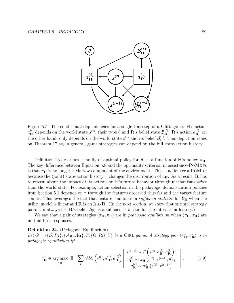
CHAPTER 5. PEDAGOGY 89
Figure 5.5: The conditional dependencies for a single timestep of a Cirl game. H’s actiona
(t)H depends on the world state s(t), their type θ and R’s belief state B(t)
R . R’s action a(t)R , on
the other hand, only depends on the world state s(t) and its belief B(t)R . This depiction relies
on Theorem 17 as, in general, game strategies can depend on the full state-action history.
Definition 23 describes a family of optimal policy for R as a function of H’s policy πH.The key difference between Equation 5.8 and the optimality criterion in assistance-PoMdpsis that πH is no longer a Markov component of the environment. This is no longer a PoMdpbecause the (joint) state-action history τ changes the distribution of aH. As a result, R hasto reason about the impact of its actions on H’s future behavior through mechanisms otherthan the world state. For example, action selection in the pedagogic demonstration policiesfrom Section 5.1 depends on τ through the features observed thus far and the target featurecounts. This leverages the fact that feature counts are a sufficient statistic for BR when theutility model is linear and R is an Irl-R. (In the next section, we show that optimal strategypairs can always use R’s belief BR as a sufficient statistic for the interaction history.)
We say that a pair of strategies (πH, πR) are in pedagogic equilibrium when (πH, πR) aremutual best responses.
Definition 24. (Pedagogic Equilibrium)Let G = 〈S, PS, AR,AH, T, Θ, Pθ, U〉 be a Cirl game. A strategy pair (π∗H, π
∗R) is in
pedagogic equilibrium iff
π∗H ∈ arg maxπH
E
∑t
γtUθ(s(t), a
(t)H , a
(t)R
) ∣∣∣∣∣∣∣s(t+1) ∼ T
(s(t), a
(t)H , a
(t)R
);
a(t)H ∼ πH
(s(t), τ (t−1); θ
);
a(t)R ∼ π∗R
(s(t), τ (t−1)
) ; (5.9)

CHAPTER 5. PEDAGOGY 90
π∗R ∈ arg maxπR
E
∑t
γtUθ(s(t), a
(t)H , a
(t)R
) ∣∣∣∣∣∣∣s(t+1) ∼ T
(s(t), a
(t)H , a
(t)R
);
a(t)H ∼ π∗H
(s(t), τ (t−1); θ
);
a(t)R ∼ πR
(s(t), τ (t−1)
) . (5.10)
Note that pedagogic equilibrium need not maximize E [Uθ]. Theorem 15 proves thisby appealing to a counter-example apprenticeship game in the Lavaland domain from Sec-tion 4.2.
Theorem 15. There exist Cirl games G with strategy pairs (πH, πR) such that
1. (πH, πR) is a pedagogic equilibrium in G; and
2. there exists an alternative strategy pair (π∗H, π∗R) that gets higher expected utility
V (π∗H,π∗R) > V (πH,πR). (5.11)
Proof. We show this by construction. Consider the Proof-of-Concept Lavaland domain fromSection 4.2 where there are 4 types of states sgrass, sdirt, starget, slava and φ(s) is a one-hotencoding of state type. Let G be an an apprenticeship game where the slava indicator isconstant in the development environment E. Suppose, additionally, that there exist typesθ0, θ1 such that
Pθ (θ0) = Pθ (θ1) ; (5.12)
U (slava, aH, aR; θ0) = −U (slava, aH, aR; θ1) ; (5.13)
U (s, aH, aR; θ0) = U (s, aH, aR; θ1) , s ∈ sgrass, sdirt, starget; (5.14)∣∣∣∣∣∣∣arg maxτ
∑(s(t),a(t))∈τ
γtU(s(t), a
(t)H , a
(t)R ; θi
)∣∣∣∣∣∣∣ > 1, i ∈ 0, 1. (5.15)
Let the deployment environment consist of two copies of E: one where the indicator forslava is on, and another where the indicator for slava is off. Call them Elavaand E¬lava. Inaddition, there is one new state s0 with 2 actions alava and a¬lava. alava samples the nextstate from the initial distribution of Elava and a¬lava samples from the initial distribution ofE¬lava.
We will now construct two pedagogic equilibria with distinct value, which will show theresult. First consider the case where πH maximizes immediate reward and breaks ties ran-domly. θ0 and θ1 will have the same likelihood in the posterior because they each inducethe same distribution of utility evaluations in the development environment. Thus, Equa-tion 5.12 and Equation 5.13 allow us to conclude that QR (s0, alava;BR) = QR (s0, a¬lava;BR)
when H maximizes utility in E. As a result, br(πβH
)can take either action in s0. Suppose
R breaks ties randomly.
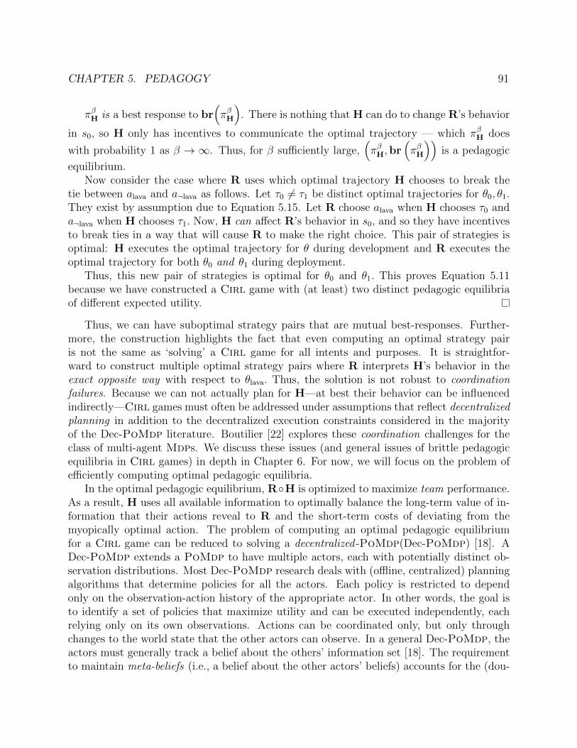
CHAPTER 5. PEDAGOGY 91
πβH is a best response to br(πβH
). There is nothing that H can do to change R’s behavior
in s0, so H only has incentives to communicate the optimal trajectory — which πβH does
with probability 1 as β → ∞. Thus, for β sufficiently large,(πβH,br
(πβH
))is a pedagogic
equilibrium.Now consider the case where R uses which optimal trajectory H chooses to break the
tie between alava and a¬lava as follows. Let τ0 6= τ1 be distinct optimal trajectories for θ0, θ1.They exist by assumption due to Equation 5.15. Let R choose alava when H chooses τ0 anda¬lava when H chooses τ1. Now, H can affect R’s behavior in s0, and so they have incentivesto break ties in a way that will cause R to make the right choice. This pair of strategies isoptimal: H executes the optimal trajectory for θ during development and R executes theoptimal trajectory for both θ0 and θ1 during deployment.
Thus, this new pair of strategies is optimal for θ0 and θ1. This proves Equation 5.11because we have constructed a Cirl game with (at least) two distinct pedagogic equilibriaof different expected utility.
Thus, we can have suboptimal strategy pairs that are mutual best-responses. Further-more, the construction highlights the fact that even computing an optimal strategy pairis not the same as ‘solving’ a Cirl game for all intents and purposes. It is straightfor-ward to construct multiple optimal strategy pairs where R interprets H’s behavior in theexact opposite way with respect to θlava. Thus, the solution is not robust to coordinationfailures. Because we can not actually plan for H—at best their behavior can be influencedindirectly—Cirl games must often be addressed under assumptions that reflect decentralizedplanning in addition to the decentralized execution constraints considered in the majorityof the Dec-PoMdp literature. Boutilier [22] explores these coordination challenges for theclass of multi-agent Mdps. We discuss these issues (and general issues of brittle pedagogicequilibria in Cirl games) in depth in Chapter 6. For now, we will focus on the problem ofefficiently computing optimal pedagogic equilibria.
In the optimal pedagogic equilibrium, RH is optimized to maximize team performance.As a result, H uses all available information to optimally balance the long-term value of in-formation that their actions reveal to R and the short-term costs of deviating from themyopically optimal action. The problem of computing an optimal pedagogic equilibriumfor a Cirl game can be reduced to solving a decentralized -PoMdp(Dec-PoMdp) [18]. ADec-PoMdp extends a PoMdp to have multiple actors, each with potentially distinct ob-servation distributions. Most Dec-PoMdp research deals with (offline, centralized) planningalgorithms that determine policies for all the actors. Each policy is restricted to dependonly on the observation-action history of the appropriate actor. In other words, the goal isto identify a set of policies that maximize utility and can be executed independently, eachrelying only on its own observations. Actions can be coordinated only, but only throughchanges to the world state that the other actors can observe. In a general Dec-PoMdp, theactors must generally track a belief about the others’ information set [18]. The requirementto maintain meta-beliefs (i.e., a belief about the other actors’ beliefs) accounts for the (dou-

CHAPTER 5. PEDAGOGY 92
bly exponential) nexp-complete time complexity of Dec-PoMdp solution algorithms [18].In the next section, we show that the commonly observed nature of s avoids this complexity.
BR is a sufficient statistic for optimal policy pairs
Nayyar, Mahajan, and Teneketzis [114] shows that a Dec-PoMdp can be reduced to acoordination-PoMdp. The actor in this PoMdp is a coordinator that observes all commonobservations and specifies a local policy for each actor called a decision rule. These policiesmap each actor’s private information to an action. The structure of a CIRL game implies thatthe private information is limited to H’s initial observation of θ. This allows the reduction toa coordination-PoMdp to preserve the size of the (hidden) state space, making the problemeasier.
Theorem 16. Let M be an arbitrary Cirl game with state space S and reward space Θ.There exists a (single-actor) PoMdp MC with (hidden) state space SC such that |SC| =|S| · |Θ| and, for any policy pair in M , there is a policy in MC that achieves the same sumof discounted rewards.
Proof. We take MC to be the coordination POMDP associated associated with M . Thesecond component of C’s action is an action for R. R has no private observations, so for anypolicy πR R could choose to follow, C can match it by simulating πR and outputting thecorresponding action. Similarly, C only observes common observations, so R can implementany coordinator strategy by simulating C and directly executing the appropriate action.
By a similar argument, H can also simulate any given πC to compute their decision rulevH, and then execute the corresponding action. To see that there is a πC that can reproducethe behavior of any πH, let h be the action-observation history for H. C can choose thefollowing decision rule
vH(θ) = πH(θ;h)
to produce the same behavior.
An immediate consequence of this result is that R’s belief about θ is a sufficient statisticfor optimal behavior.
Theorem 17. Let M be a Cirl game. There exist optimal policies (π∗H, π∗R) that only
depend on the current state and R’s belief.
πH∗ : S ×∆ (Θ)×Θ→ AH, πR
∗ : S ×∆ (Θ)→ AR.
Proof. [149] showed that an optimal policy in a PoMdp only depends on the belief state.R’s belief uniquely determines the belief for C. From this, an appeal to Theorem 16 showsthe result.

CHAPTER 5. PEDAGOGY 93
Remark 10. In a general Dec-PoMdp, the hidden state for the coordinator-PoMdp in-cludes each actor’s history of observations. In Cirl, θ is the only private information sowe get an exponential decrease in the complexity of the reduced problem. This allows one toapply general PoMdp algorithms to compute optimal joint policies in Cirl.
It is important to note that the reduced problem may still be very challenging. PoMdpsare difficult in their own right and the reduced problem still has a much larger action space.That being said, this reduction is still useful in that it characterizes optimal joint policycomputation for Cirl as significantly easier than Dec-PoMdps. Furthermore, this theoremcan be used to justify approximate methods (e.g., iterated best response) that only dependon R’s belief state.
A efficient dynamic programming algorithm for CIRL
Next, we will build on this result to design efficient (approximate) dynamic programmingmethod for Cirl games. The previous reduction greatly simplifies the belief space thatmust be considered during (joint) policy optimization. However, this comes at the cost ofmuch larger action space. This is because the action space in the coordination PoMdp isthe product of R’s action space AR and the set of mapping from H’s type to their actionspace. This leads to an action space in the coordinator PoMdp with |AR| · |AH||Θ| distinctactions to be considered. To counteract this blowup, we can take advantage of the specialinformation structure of a Cirl game. H is a full-information actor and so, although theirpolicy is not Markov with respect to the environment state, it can be computed exactly fromintermediate calculations already used in PoMdp value iteration.
A cooking assistance game
We will introduce our method with the use of an example cooking assistance game. In thisgame, R and H are working together to make food. There are several ingredients that canbe prepared to cook recipes. H’s type space Θ is the set of possible recipes.
Take for instance the domain from Figure 5.6. H and R work to prepare a meal usingthree ingredient types: bread, meat, and tomatoes. H wants to prepare either a sandwich(2 bread, 1 meat, 0 tomatoes), or tomato soup (1 bread, 1 meat, 2 tomatoes). R does notknow a priori which meal H wants. At every time step, R and H each prepare a single unitof any ingredient, or no ingredient at all. The state produces utility 1 if the desired recipehas been made and 0 otherwise. In this domain, (optimal) pedagogic equilibrium modelsH’s incentive for the robot to infer the correct recipe. The structure of Θ allows R to act,at least initially, based on incomplete information about the correct recipe: bread and meatare a good idea for either recipe.

CHAPTER 5. PEDAGOGY 94
Figure 5.6: An example of the cooking domain. H and R need to work together to prepare ameal using H’s desired recipe. R starts off unaware of which meal H wants. In our runningexample, there are 3 types of ingredients: bread, meat, and tomatoes. There are 2 recipes:a sandwich (2 bread, 1 meat, 0 tomatoes) and tomato soup (1 bread, 1 meat, 2 tomatoes).The world state represents how many (0, 1, or 2) of each ingredient has been prepared. Ina pedagogic solution for this game, H chooses to make tomatoes first if they want tomatosoup; the other ingredients are needed for both recipes, so R can make either. R can theninfer that H wants a sandwich if they make bread, because they would have made tomatoesotherwise. This pragmatic reasoning on R’s part is a distinguishing property of pedagogicequilibrium in assistance games. No Irl-R can make this inference because bread is neededfor both recipes.
Cooking as an Assistance-POMDP
Before introducing our approach, we describe value iteration as it applies to assistance-PoMdps. As discussed in Chapter 2, value iteration algorithms often track a set of poten-
tially optimal conditional plans. We write a conditional plan as σ =(a
(t)R , v
(t))
. a(t)R ∈ AR
indicates R’s next action. v(t) maps the current observation, H’s action a(t)H , into the next
conditional plan.The value of a conditional plan depends on the associated belief state BR. A useful
observation for PoMdp algorithms is that this can be represented efficiently as a vector ofvalues: one for each possible hidden state. In an assistance-PoMdp, this is a mapping from

CHAPTER 5. PEDAGOGY 95
Θ the value of the given conditional plan when H has that type.The α-vector of a conditional plan σ = (aR, v) in a assistance-PoMdp, is defined by the
following dynamic programming relationship:
ασ (s; θ) = E
[U (s, aH, aR; θ) + γ
∑s′∈S
T (s′ |s, aH, aR )αv(aH) (s′; θ)
∣∣∣∣∣ aH ∼ πH (s; θ)
]. (5.16)
The value of a plan at a belief BR is the expected value of the plan across the states i.e.V σ(BR) = BR · ασ =
∑s∈S BR (s) · ασ (s). The goal of an agent in a PoMdp is to find the
plan with maximal value from their current belief.Value iteration [153] can be used to compute the optimal conditional plan. This algorithm
starts at the horizon and works backwards. It generates new conditional plans at each time-step and evaluates them according to Equation 5.16. It constructs all potentially optimalplans of a given length, set in relation to γ to ensure optimality, and selects the one withmaximal value at the initial belief.Solving an assistance-PoMdp for cooking. For example, consider a simplified instanceof the cooking task from Figure 5.6 where H picks their actions according to only theirdesired recipe and the quantity of each ingredient prepared so far, i.e., they do not considerR’s past or future behavior when picking their actions. The simplified cooking task is nowan assistance-PoMdp. I.e., H is modeled as a Markov component of the environment.BR is a distribution over possible recipes, in this case over the set Sandwich,TomatoSoup.
R’s behavior is specified by a conditional plan σ = (a, v). For example,
σ =
Bread,
Bread→ (Meat, ∅) ## Target recipe: Sandwich
Tomatoes→ (Meat,Tomatoes) ## Target recipe: TomatoSoup
Meat→ (∅, v′) ## Target recipe: ??
.
(5.17)This is one component of a conditional plan for an Irl-R. R prepares bread first, because itis needed for both recipes. If H makes bread, then we know the desired recipe is a sandwich.R prepares the final piece of bread to complete the sandwich. If H makes tomatoes, thenthe recipe is tomato soup, and R H finishes the recipe in the next round. However, if Hresponds by preparing meat, θ is not identified. R must make a guess at the next action,potentially wasting food, time, or both. In this case, recipe completion proceeds accordingto the decision rule v’.
Note that σ is a best response to πH in this example and πH chooses actions that areoptimal for H in isolation. Thus, Equation 5.17 is an optimal solution to the assistance-PoMdp formulation of the cooking problem. The ultimate value of the policy comes downto details of how H breaks ties between optimal-in-isolation actions. If H would simplyadopt the policy
vPedagogy = Sandwich→ Bread; TomatoSoup→ Tomatoes, (5.18)
then the target recipe is guaranteed to be made in two rounds (as opposed to 3). In the nextsection, we will show how Cirl model’s H’s incentives to make this change.

CHAPTER 5. PEDAGOGY 96
;
;
Figure 5.7: A node in the search tree from the PoMdp reduction of the ChefWorld domain.Actions are tuples that contain an action for R and a decision rule for H – a mapping fromtheir desired recipe to an action. This leads to a branching factor of |AH||Θ||AR| and makesapplication of PoMdp methods inefficient. The modified Bellman update from Section 5.2prunes away all of H’s decision rules but the optimal response. (In the diagram, the graybranches are pruned away by the modified Bellman update.)
The Coordination-POMDP for cooking
Now, consider what changes when we model the problem as a Cirl game. H’s policy cannow account for R’s conditional plan σ. H can select actions in response to Qσ
θ . Thus,they recognize the suboptimality of preparing meat initially. This causes them to followEquation 5.18, increasing the expected utility from the interaction.
However, this comes at a computational cost. Consider the coordination-PoMdp re-duction for this example. The action space has become much larger. It must specify anaction for R aR and a decision rule vH for H. The size of the action space for the cook-ing assistance-PoMdp is 4: one action for each ingredient and an additional no-op, ∅. Theaction space in the coordination-PoMdp increases this to 32 = 25: there are |AH||Θ| = 42
distinct decision rules for H which can each be paired with a different aR. Figure 5.7 showsan illustration of this action space as a tree.

CHAPTER 5. PEDAGOGY 97
The computational efficiency of an assistance-PoMdp formulation (and the associatedapproximation) is clear. H’s component of the action can be marginalized over if they aremodeled as a Markov observation model. The key insight we leverage in our approach isthat it is still possible to do this marginalization even if H’s behavior depends on V σ
θ .
Theorem 18. Let G = 〈S, PS, AR,AH, T, Θ, Pθ, U〉 be a Cirl game. H’s valuefunction for a conditional plan σ is equal to ασ. That is, for any conditional plan σ andθ ∈ Θ
V σθ (s) = ασ (s; θ) . (5.19)
Proof. This follows directly from the definition of ασ as the vector of values for σ as afunction of the latent state (s, θ).
In a general Dec-PoMdp computing the value function for any actor requires taking adot product with their belief. However, full-information actors have a very restricted class ofpossible beliefs: beliefs that place all their mass on a single state. Thus, ασ tracks the valuefunction of full-information actors. This means that fully-informed, cooperative, strategicbehavior can be accounted for with minimal increase in computational complexity.
Specifically, we can update the dynamic programming relationship in Equation 5.16 toaccount for H’s strategic behavior by maximizing over aH:
ασ (s; θ) = maxaH∈AH
U (s, aH, aR; θ) + γE
[αv(aH) (s′; θ)
∣∣ s′ ∼ T (s, aH, aR)]. (5.20)
Corollary 18.1. For any Cirl game G, the policy computed by value iteration with Equa-tion 5.20, π∗R is a component of an optimal pedagogic equilibrium (π∗H, π
∗R).
Proof. From Theorem 18, we know that H’s value function for a given conditional plan σ isgiven by ασ. Thus, the maximization in Equation 5.20 never prunes away an optimal actionfor H. Thus, the conditional plan output at the end of value iteration, which is the bestpolicy among those not pruned away, must be optimal.
This modification to the Bellman update allows us to solve a Cirl game without havingto include the set of H’s decision rules in the action space. As depicted in Figure 5.7,the modified Bellman update computes H’s optimal action given the current state and therobot’s plan; all of H’s other actions are pruned away in the search tree. The size of theaction space is then |AR| instead of |AH||Θ||AR|. PoMdp algorithms are exponential in thesize of the action space; this modification therefore allows us to solve Cirl games much moreefficiently. The following theorem establishes the associated complexity gains.
Theorem 19. The modification to the Bellman update presented above reduces the time andspace complexity of a single step of value iteration by a factor of O
(|AH||Θ|
).

CHAPTER 5. PEDAGOGY 98
Algorithm 1 Adapted Value Iteration for CIRL Games
1: procedure ValueIteration2: Γt ← Set of trivial plans3: for t ∈ T − 1, T − 2, . . . , 1, 0 do4: Γt+1 ← Γt5: Γt ← Set of all plans beginning at time t6: for σ ∈ Γt do7: for s = (x, θ) ∈ S do8: QH(s, aH , σ) =
∑s′ T (s, aH , aR, s′) · αv(aH)(s
′)9: ασ(s) = R(s) + γ ·∑aH πH(aH | QH(s, aH , σ)) ·QH(s, aH , σ)
10: Γt ← Prune(Γt)
11: aR∗ = arg maxσ∈Γ0ασ · b0
12: Return aR∗
Proof. The complexity of one step of POMDP value iteration is linear in the size of theaction space, |A| [129]. Since the structure of our algorithm is identical to that of exactvalue iteration, this is also true for our algorithm.
The action space in the POMDP reduction of CIRL has size |AH||Θ||AR|. Our modifica-tion to the Bellman update reduces the size of the action space to simply |AR|. Therefore,our algorithm reduces the time taken to run, and number of plans generated at, each timestep by a factor of |AH||Θ|.
Our experimental domain is based on the cooking example. Assume there are m recipesand n ingredients. The state space is an n-tuple representing the quantity of each ingredientprepared thus far. At each time step, each agent can prepare any of the n ingredients ornone at all. Each of the m recipes corresponds to a different θ (i.e. reward parameter) value.Both agents receive a reward of 1 if H’s desired recipe is prepared correctly and a rewardof 0 otherwise. The robot R begins the game entirely uncertain about H’s desired recipei.e. R has a uniform belief over Θ. In our first experiment, we compared the time takenby exact VI and by our adaptation of it with the modified Bellman update. We first fixedthe number of ingredients at two and varied the number of recipes in the domain. Table 5.2compares the results. For the simpler problems, where the number of recipes was 2 or 3, ouradapted algorithm solved the problem up to ∼3500× faster than exact VI. On more complexproblems where the number of recipes is greater than 3, exact VI failed to solve the problemafter depleting our system’s 16GB memory; in contrast, our adapted algorithm solved each ofthese more complex problems in less than 0.5 seconds. We next fixed the number of recipesand compared the performance of both these algorithms for various numbers of ingredients.Both the exact methods, but especially the one using the standard Bellman update, scaledmuch worse with the number of ingredients than with the number of recipes. With eventhree ingredients, exact VI timed out and failed to solve the problem within two hours; ouralgorithm however solved the problem in five seconds.

CHAPTER 5. PEDAGOGY 99
Table 5.2: Time taken (s) to find the optimal robot policy using exact VI and our adaptationof it for various numbers of possible recipes. NA denotes that the algorithm failed to solvethe problem.
# Recipes Exact VI Ours2 4.448 ± 0.057 0.071 ± 0.0133 394.546 ± 6.396 0.111 ± 0.0134 NA 0.158 ± 0.0035 NA 0.219 ± 0.0076 NA 0.307 ± 0.005
Comparing CIRL and IRL solutions
Next, we consider what advantages Cirl has compared to Irl. On a collaborative task, Irlis equivalent to assuming that H chooses their actions in isolation, and R uses observations ofH’s behavior to infer their preferences. Specifically, H solves a single-agent, fully-observable,variant of the problem, and R responds by solving the appropriate assistance-PoMdp.
We fix the number of ingredients at 3 and vary the number of recipes. Figure 5.8 shows theresults. In each experiment the optimal Cirl solution prepares the correct recipe while theIrl solution fails to do so up to 50% of the time. To understand the nature of this differencein performance, we analyze the Cirl and Irl solutions. Consider a case of our runningexample from before with two recipes. The state is a tuple (#meat,#bread,#tomatoes)and Θ = sandwich = (1, 2, 0), soup = (1, 1, 2). For both approaches, R initially preparesmeat. In the baseline IRL solution, H can initially make any ingredient if they want soupand can make meat or bread if they wants a sandwich. In each case, H chooses uniformlyat random between allowed ingredients. This conveys some information about their desiredrecipe, but is not enough to uniquely identify it. Since the same ingredient is optimal formultiple recipes, R is still confused after one turn. This means R will sometimes fail tocomplete the desired recipe, reducing average utility.
The Cirl solution, in contrast, relies on the implicit communication between the humanand the robot. Here, if H wants soup, she prepares tomatoes, as opposed to any ingredientsthat are common with the sandwich. Even more interestingly, she waits (i.e. does nothing)if she wants a sandwich. This is pure signaling behavior—waiting is suboptimal in isolation,but picking an ingredient is more likely to confuse the robot. In turn R knows that H wouldhave picked tomatoes if she wanted soup, and responds appropriately.
In other words, H teaches the robot about her preferences with her action selection. Thisworks because H knows that R will interpret her behavior pragmatically, i.e., R expects tobe taught by H. This is reflected in the experiment: the optimal Cirl solution prepares thecorrect recipe each time.
The value alignment problem is necessarily cooperative: without the robot, the human is

CHAPTER 5. PEDAGOGY 100
Figure 5.8: Value attained by Cirl and standard Irl on the cooking domain with variousnumbers of possible recipes. Unlike Irl, Cirl produces solutions where H picks their actionspedagogically and R reasons about H accordingly.
unable to complete her desired task, and without explicit signaling from the human, the robotlearns inefficiently, is less valuable and is more likely to make a mistake. Pedagogic behaviorfrom H naturally falls out of the Cirl solution. In response, R interprets H’s actionspragmatically. These instructive and communicative behaviors allow for faster learning andcreate an opportunity to generate higher value for the human.
Efficient Approximate Algorithms for CIRL
Adapting Point-Based Value Iteration
Background Point Based Value Iteration (PBVI) is an approximate algorithm used to solvePOMDPs [121]. The algorithm maintains a representative set of points in belief space andan α-vector at each of these belief points. It performs approximate value backups at each of

CHAPTER 5. PEDAGOGY 101
these belief points using this set of α-vectors. Let Γt+1 denote the set of α-vectors for plansthat begin at time t+ 1. The value at time t at a belief b is approximated as:
V (b) = maxa∈A
[∑s∈S
R(s)b(s) + γ∑o∈O
maxα∈Γt+1
∑s∈S
(∑s′∈S
P (s′, o | s, a)α(s)
)b(s)
]. (5.21)
The algorithm trades off computation time and solution quality by expanding the set of beliefpoints over time: it randomly simulates forward trajectories in the POMDP to produce new,reachable beliefs.Our Adaptation If R takes action aR and follows a conditional plan σ, then H’s Q-valuesare QH(x, aH, aR, α) =
∑s′ T (s, aH, aR, s
′) · ασ(s′). Notice that we can compute these Q-values at each step of PBVI. This lets us use the modified Bellman update and to adaptPBVI to solve CIRL games specifically. We replace the transition-observation distributionin the PBVI backup rule with
P (s′, aH | s, aR, α) = T (s, aH, aR, s′) · πH(QH(x, aH, aR, α)). (5.22)
The modified backup rule for PBVI is thus given by
V (b) = maxaR∈AR
[∑s∈S
R(s)b(s) + γ∑aH
maxα∈Γt+1
∑s∈S
(∑s′∈S
P (s′, aH | s, aR, α)α(s)
)b(s)
]. (5.23)
We now show that the approximate value function in PBVI converges to the true valuefunction. Let εB denote the density of the set of belief points B in PBVI. Formally, εB =maxb∈∆ minb′∈B ||b− b′||1 is the maximum distance from any reachable, legal belief to the setB.
Theorem 20. For any belief set B and horizon n, the error of our adapted PBVI algorithmη = ||Vn − V ∗n ||∞ is bounded as
η ≤ (Rmax −Rmin)εB(1− γ)2
.
Proof. Since the dynamics of our problem are now time-varying instead of static, the backupoperator applied at every time-step changes. Let Ht denote the backup operator applied tocompute the value of Vt. It will suffice to show that each such backup operator Ht is acontraction mapping. The result then follows by following the proof of Theorem 1 in [121]exactly. We will prove the result by showing that each Ht is the backup operator for aspecific POMDP and thus, for this POMDP’s corresponding belief MDP; it must thereforebe a contraction mapping.
Take Ht for some 1 ≤ t ≤ n. We will now construct a new POMDP for which Ht
is the backup operator. Let S = S × Γt+1, where Γt+1 denotes the set of α-vectors fromour original problem at time t + 1. Let the α-vector component of the state be static i.e.

CHAPTER 5. PEDAGOGY 102
P ((s′, α′) | (s, α), aR) = 0 if α 6= α′. The action and observation spaces remain as they arein our original problem. The transition-observation distribution, given in Eqn. (3), is nowtime-invariant: we do not need to look forward in the search tree to compute the Q-valuessince the α-vectors are available in the state space. Hence, this POMDP is well-defined.
The dynamics of the POMDP are static and identical to the dynamics of our problemat time t. Thus, the backup operator Ht is the backup operator for this POMDP and alsofor this POMDP’s corresponding belief MDP. Therefore, the backup operator Ht must be acontraction mapping.
Next, we compared the values attained by PBVI and our adaptation, with one hour ofcomputation time. We first fixed the number of recipes and varied the number of ingredi-ents. The results of this experiment are presented in Figure 5.9. We found that both thesealgorithms, but especially our adapted algorithm, scaled much better with the number ofingredients than their exact VI counterparts. For simpler games, with 3 and 4 ingredients,both algorithms attained the maximal value of 0.9025. However, with 5 ingredients, PBVIfound a value of 0 in an hour. In contrast, our algorithm easily solved the game with 5,6, and 7 ingredients, attaining the maximal value of 0.9025. We next fixed the number ofingredients and varied the number of recipes. Again, our adapted algorithm outperformedPBVI. For example, with 4 recipes, our adapted method attains a value of 0.67875 while thestandard PBVI method attains a value of 0.45125.
These results suggest that our modified Bellman update allows PBVI to scale to largerCIRL games, especially in terms of the size of H’s and R’s action space. This offers furthersupport to our hypothesis.
Adapting Partially-Observed Monte-Carlo Planning
Background POMCP is a Monte Carlo tree-search (MCTS) based approximate algorithmfor solving large POMDPs [143]. The algorithm constructs a search tree of action-observationhistories and uses Monte Carlo simulations to estimate the value of each node in the tree.During search, actions within the tree are selected by UCB1. This maintains a balancebetween exploiting actions known to have good return and exploring actions not yet taken[89]. At leaf nodes, a rollout policy accrues reward which is then backed up through the tree.The algorithm estimates the belief at each node by keeping track of the hidden state fromprevious rollouts.
POMCP scales well with the size of the state space, but not with the size of the actionspace, which determines the branching factor in the search tree. POMCP is thus ill-suited tosolving the reduced POMDP of CIRL games since the size of the action space is |AH||Θ||AR|.Our Adaptation Using the idea behind our modified Bellman update, we adapt POMCP tosolve CIRL games more efficiently. We approximate H’s policy while running the algorithm(much like we exactly compute H’s policy in exact value iteration). We maintain a liveestimate of the sampled Q-values for H at each node. With enough exploration of the searchtree (for instance, if actions are selected using UCB1), the estimated Q-values converge to

CHAPTER 5. PEDAGOGY 103
Algorithm 2 Adapted PBVI for CIRL Games
1: procedure PBVI(b0, T )2: B ← b03: V ← Set of α-vectors belonging to trivial plans4: repeat5: for t ∈ T − 1, T − 2, . . . , 1, 0 do6: V ← Backup(B, V )
7: B ← Expand(B, V )8: until maxα∈V α · b0 ≥ Vtarget9: return V
10:
11: procedure Backup(B, V ′)12: V ← 13: for aR ∈ AR do14: for α′i ∈ V ′ do15: for s ∈ S do16: QH(s, aH) =
∑s′ T (s, aH , aR, s′)·
17: αv(aH)(s′)
18: ΓaR ← αi(s) = r(s) + γ·
19:∑
aH πH(aH | QH(s, aH))·20:
∑s′ P (s′, aH | s, aR, α′i) · αi(s′)
21: for b ∈ B do22: Vb ← 23: for aR ∈ AR do24: Vb ← argmaxα∈ΓaRα · b25: V ← argmaxα∈Γbα · b26: return V27:
28: procedure Expand(B′, V ′)29: B ← B′
30: for b, α ∈ B′, V ′ do31: Bb ← 32: for aR ∈ AR do33: s ∼ b(s)34: aH ∼ P (aH | s, aR, α)35: b′(s′) = η
∑s P (s′, aH | s, aR, α)b(s)
36: where η is the normalizing constant37: Bb ← Bb ∪ b′38: B ← B ∪ argmax||b− b′||1,∀b ∈ Bb, b
′ ∈ B′39: return B

CHAPTER 5. PEDAGOGY 104
Figure 5.9: Value attained by PBVI and our approximate algorithm for various numbers ofingredients. (For the first 3 data points, the values attained by both methods were the same– we jittered the plot slightly for visibility).
the true values (in the limit). This guarantees that H’s policy converges to her true policy.The following result establishes convergence of our algorithm.
Theorem 21. With suitable exploration, the value function constructed by our adaptedPOMCP algorithm converges in probability to the optimal value function, V (h)→ V ∗(h). Asthe number of visits N(h) approaches infinity, the bias of the value function E[V (h)−V ∗(h)]is O(log(N(h))/N(h)).
Proof. We will show that with enough exploration, in the limit of infinite samples, we havea well defined POMDP. The result then follows from Theorem 1 in [143].
The human action nodes in the search tree maintain an array of values, which store thevalues of picking that action for different θ. At any point in the search tree, the human actions

CHAPTER 5. PEDAGOGY 105
(like the robot actions) are selected by picking the one that has the maximum augmentedvalue (current estimated value plus exploration bonus). So, in the limit of infinite samples,each human action node is visited infinitely many times and the value estimates at the nodesconverge to the true Q values. Having the correct human Q values gives us a POMDP, withwell defined transition-observation dynamics. The result then follows from applying theanalysis given in Theorem 1 of [143] to this POMDP.
We compared the value attained in 30,000 samples by POMCP and by our adaptationwith the modified Bellman update. We additionally compared these algorithms with FV-POMCP, a state-of-the-art MCTS method for solving MPOMDPs, a type of Dec-POMDPin which all agents can observe each others’ behavior (as in CIRL).
We first fixed the number of recipes at 2 and varied the number of ingredients. Ouradapted algorithm outperformed the other two algorithms across the board, especially forlarge numbers of ingredients. The results of this comparison are presented in Figure 5.10.POMCP did poorly on games with more than 4 ingredients. Although FV-POMCP scaledbetter to more complex games than POMCP, its values had high variance. For the largestgames, with 6 and 7 ingredients, our adapted algorithm was the only one capable of solvingthe problem in 30,000 iterations. We also compared the value attained by each algorithmacross 500,000 samples on the 6 ingredient game. The results of this comparison are depictedin Figure 5.11. Our algorithm converged to the true value faster than either of the otheralgorithms.
We next fixed the number of ingredients at 4 and varied the number of recipes. We foundthat the results of this experiment broadly matched the results of our previous experimentwhere we varied the number of ingredients. For example, with 4 recipes, our method achievesan average value of 0.631± 0.221 in 30,000 iterations while POMCP gets 0.429± 0.183 andFV-POMCP gets 0.511± 0.124.
Next, we also applied POMCP to a more complex domain. This domain is an extensionof the POMDP benchmark domain RockSample, that models Mars-rover exploration [150].Consider a collaborative task where a human H wants to take samples of some rocks fromMars, with the help of a rover R deployed on Mars. There are some number of hours duringthe day (working hours) when H can control R herself but for the rest of the day, R has tobehave autonomously. Not all types of rocks are of equal scientific value; H knows the valueof each of these rocks but R does not. (Once again, we assume that H cannot communicatethese values to R directly.)
Formally, consider an instance of RockSample on a m × m grid, with n rocks, each ofwhich belong to one of k different types. The state space is a cross-product of the x- andy-coordinate of R with n binary features IsSampledi = Y es,No, which indicate which ofthe rocks have already been sampled. (Each rock can only be sampled once.)
RockSample is a turn-based game: R may first take lR steps in any of the four cardinaldirection (during those hours when it is running autonomously) after which H may similarlytake lH steps (during the remaining hours). Thus, the set of actions available to H is the setof all trajectories of length exactly lH while that available to R is the set of all trajectories

CHAPTER 5. PEDAGOGY 106
Algorithm 3 Adapted POMCP for CIRL games
1: procedure Search(h)2: repeat3: if h = empty then4: s ∼ I5: else6: s ∼ B(h)
7: Simulate(s, h, 0)8: until Timeout()9: return argmaxaRV (haR)
10:
11: procedure Rollout(s, h, depth)12: if γdepth < ε then13: return 014: aR, aH ∼ Uniform(AR), Uniform(AH)15: s′ ∼ T (s, aR, aH)16: return r(s) + γ ·Rollout(s′, haRaH , depth+ 1)
17:
18: procedure Simulate(s, h, depth)19: if γdepth < ε then20: return 021: if h /∈ T then22: return Rollout(s, h, depth)
23: aR ← argmaxaRV (haR) + c√
logN(h)N(haR)
24: θ ← sθ25: aH ← SampleHumanAction(θ, h, aR)26: s′ ∼ T (s, aR, aH)27: R← r(s) + γ · Simulate(s′, haRaH , depth+ 1)28: B(h)← B(h) ∪ s29: N(h)← N(h) + 130: N(haR)← N(haR) + 131: N(haRaH)← N(haRaH) + 1
32: V (haR)← V (haR) + R−V (haR)N(haR)
33: Vθ(haRaH)← Vθ(ha
RaH) + R−Vθ(haRaH)Nθ(haRaH)
34: return R35:
36: procedure SampleHumanAction(θ, h, aR)
37: aH ∼ πH
(aH | Vθ(haRaH) + c
√logNθ(haR)Nθ(haRaH)
)38: return aH

CHAPTER 5. PEDAGOGY 107
Figure 5.10: The value attained by POMCP, FV-POMCP, and our adapted algorithm in30,000 samples with various numbers of ingredients. (Right) Value attained by POMCP,FV-POMCP and our approximate algorithm with 2 recipes and 6 ingredients.
with length at most lR. (R may wait on any specific step if it requires more informationwhile H may not wait since they has all the information required.)
The set of all reward parameters Θ is composed of a collection of k-dimensional vectors,where the ith entry represents the reward received for sampling rock i. Both agents receivethe reward specified by the true reward parameter θ when they sample a rock and receiveno reward for any other action.
Details of Experiment
We repeated our experiment with a 5× 5 grid (m = 5), 3 types of rocks (k = 4), and 4 rockstotal (n = 4).
This domain is much more complex than the cooking domain. For example, note that foreven the simplest version of this domain, with lH = lR = 1, |AH| = 4 and |AR| = 5 (since R

CHAPTER 5. PEDAGOGY 108
Figure 5.11: Value attained by POMCP, FV-POMCP and our approximate algorithm with2 recipes and 6 ingredients.
can also choose to wait); if we raise lR slightly to 2, we have |AR| = 13. Hence, we only ranour experiments with POMCP, which scales the best of the three types of the algorithms.
We found similar results to those from ChefWorld. For any value of lR beyond 1, FV-POMCP and POMCP fail to solve the problem; the branching factor of the search treethey both construct is too large and thus, both methods deplete the 16GB of memory inour system almost immediately. Our method however manages to scale to larger values oflH and lR with relative ease; our method successfully computed the optimal policy for thisdomain with values of lH = lR = 2 within two hours of computation.

109
Chapter 6
Robust Alignment
This chapter discusses the equilibrium selection problem that can arise in assistance gamesand the need to consider strategy robustness in the study of assistance games. The chapterbegins with an application of the tools from the previous chapter to compare the performanceof pedagogic solutions with individual reward maximizing solutions. As one might expect,pedagogic solutions lead to higher utility for H. Because even the pedagogic H still has topay a lot of attention to immediate reward, R’s best-response still performs well even if His not behaving pedagogically.
Next, we consider a setting that admits purely pedagogic solutions that have no connec-tion to immediate reward. The setting is a modification of the supervision problem fromSection 3.1 where H needs to learn which actions produce reward from experience. BecauseH’s actions only impact R’s information state, all actions produce the same immediatereward in an assistance game formulation.
We will show that there exists a class of solutions where H acts as if R will copy theiraction and approximately maximizes the expected reward of their selections given the rewardobservations so far. A single strategy for R that occasionally takes exploration actions for Hcan successfully assist any strategy for H from this family of alternatives. This represents arelatively robust alignment solution: the combined system RH is guaranteed to eventuallytake the optimal action with probability 1, so long as H satisfies relatively simple constraintson their policy.
These solutions, however, may take arbitrarily long to settle on the optimal action. As inCirl, R H can perform better if H reveals more information about their goal. In this casehowever, the best H can do is reveal information about their history of reward observations.In some cases, H may be able to communicate enough information that R can behave asif it directly observes reward. This means that R H can implement the optimal learningstrategy.
However, this performance improvement comes at the cost of robustness. Because H onlycares about how R interprets their actions, there are multiple distinct pedagogic solutionsthat arise from equally informative but distinct ways to encode their reward observations.Furthermore, misalignment in these encoding schemes can lead R H to perform arbitrarily

CHAPTER 6. ROBUST ALIGNMENT 110
poorly, even though H’s behavior reveals a lot of information about their goal. In the worstcase, R H may even minimize utility for H. This is unlike the ChefWorld example, wherethe pedagogic solutions needed to be informative and maximize immediate reward. As aresult, we consider two additional modes of interaction: a turn-taking mode where H andR alternate choosing arms, and a preemptive mode, where R decides to pull an arm orask H to pull an arm. As one might expect, the communicative policy WSLS is now lessattractive — although other, more complicated, communication strategies may do a betterjob of trading off between conveying information and maximizing utility. Although the needto consider both sources of utility typically increases the burden on H it can help managealignment problems by making it easier for H and R to coordinate.
6.1 Exploring strategy robustness in ChefWorld
To further investigate the performance of Cirl-inspired alignment solutions in realistic set-tings (e.g., where H may not be rational and H’s strategy is not known perfectly in advance),we ran another experiment. We varied whether H behaved according to Cirl or Irl, R’smodel of H in training (rational or Boltzmann-rational), and the actual model of H (sameas previous). We measured the proportion of times the team prepared the correct recipe ineach setting, fixing the number of ingredients at 3 and recipes at 4. Figure 6.1 shows theprimary results.
Averaged across different models of H used to train R, when H behaved according toCirl, H and R succeeded in preparing the correct recipe > 90% of the time. This was alsotrue when H behaved Boltzmann-rationally. This suggests that the pedagogic behavior thatarises from Cirl makes it more robust to any sub-optimality from H. In contrast, when Hbehaved as in Irl (i.e., not pedagogically), they only prepared the correct recipe ∼70% ofthe time when H was rational, and ∼40% of the time when H was not. So, the importanceof pedagogic behavior from H to achieve value alignment is clear.
Additionally, these results suggest that the pedagogic behavior that arises from Cirlmakes it more robust to sub-optimality from H. When H demonstrated sub-optimal behaviorbut behaved pedagogically according to Cirl, H and R were only ∼2% less successful atpreparing the correct recipe than if H behaved optimally; however, when H demonstratedsub-optimal behavior but behaved according to Irl, they were ∼40% less successful.
To further investigate the properties that lead to effective alignment, and the conse-quences of strategy mismatch, we did a second study with 10 possible human policies in-stead of 2. The 10 policies were chosen from a 5 × 2 factorial of the human’s behavior andpresence of bias. The 5 possible behaviors were rational, Boltzmann-rational with β = 1,Boltzmann-rational with β = 5, ε-greedy with ε = 0.1, and ε-greedy with ε = 0.01. The 2possible levels for presence of bias were ”No Bias” and ”Bias”, where ”Bias” denoted thatH had a systematic preference for choosing the ”Wait” action. (In our setting, H receiveda reward of 0.25 every time they chose the ”Wait” action.)

CHAPTER 6. ROBUST ALIGNMENT 111
Figure 6.1: The proportion of times that H and R prepared the correct recipe on the cookingdomain when R is trained with, and H actually behaves according to, a variety of differentbehaviors. They were significantly more successful at preparing the correct recipe when Hbehaved pedagogically according to Cirl.
The results of our experiment are presented below in Figure 6.2 as a heat map. Much likethe simpler experiment, we find that H and R are much more successful when H behavespedagogically and that in the presence of pedagogic behavior, the team’s performance ismore robust to any sub-optimality from H.
6.2 Assisting a Learning H
Next, we turn to the problem of strategy robustness in earnest. We consider a setting whereH is subject to additional informational constraints. Namely, we assume that H has to learnabout θ from observations of reward over time. This changes the nature of R’s strategy.Instead of observing H in order to learn about θ, R also has to account for H’s informationstate. It is only after H makes enough observations about reward that their behavior canbe effectively learned from. We illustrate the difference between assisting a learner and anexpert with an example.

CHAPTER 6. ROBUST ALIGNMENT 112
Figure 6.2: The proportion of times that H and R prepared the correct recipe on the cookingdomain with 3 ingredients and 4 recipes when R is trained with, and H actually behavesaccording to, a variety of different behaviors. They were significantly more successful atpreparing the correct recipe when H behaved pedagogically by following a policy specifiedby Cirl.

CHAPTER 6. ROBUST ALIGNMENT 113
At the start of every day, the human H would like to consume a single caffeinatedbeverage, either coffee or tea. Before the human wakes up, the robot can prepare one ofthe two caffeinated beverages or choose not to. If the robot does not make a beverage, thenthe human will prepare one of the two beverages. The human has an unknown but fixedpreference toward either coffee or tea, represented by Θ = 0, 1. The human and the robotshare a uniform prior over Θ. The human gets θ reward for consuming tea and 1− θ rewardfor consuming coffee, which they will observe after consuming either the tea or coffee. Inaddition, the act of preparing coffee or tea costs the human ε = 0.1 points of reward, but ifthe tea or coffee was already prepared by the robot R, then no such penalty is incurred.
If the human knew the true value of θ in the above example, then she can maximizereward by preparing tea when θ = 1 and coffee when θ = 0. The best policy for therobot would then be wait one day to see what beverage the human chooses, then make thatbeverage every day after that. However, if the robot performs this policy when the humandoes not know the true value of θ, then this policy will lead to an expected reward of 0.5a day, lower than the 0.9 that the human can achieve if the robot always takes no action.Instead, the optimal policy for the robot would be to prepare a drink for the human — tohelp the human to learn the value of θ — and then let the human prepare a drink so thehuman can signal the value to the robot. This policy has expected reward 1 a day for eachday after the second.
Interestingly, R can help H perform better even if the cost ε of making beverages for thehuman is 0, if H is not following the optimal (reward-maximizing) policy, as the followingexample demonstrates. Suppose that the cost of making beverages for the human is ε = 0,and that the human H is a Q-learner with initial value −1 that follows a greedy policyfor choosing tea or coffee. Thus, H makes tea with probability 1 if H’s Q-value for teais higher, and vice versa in the case where their Q-value for coffee is higher (in the casewhere their Q-values are equal, they chooses one at random). No matter what beverage theysample randomly in the first timestep, H will always make that beverage afterwards due toa bad initialization and under-exploration. This leads to an average reward per episode of0 with probability 0.5. However, if R prepares both beverages, H’s Q-values will update toreflect which beverage they like better. In turn, this allows R to observe H’s preference andeventually produce utility at the optimal rate.
The key observation here is that R’s optimal policy depends meaningfully on H’s in-formation state. If R overestimates the information H can provide about rewards, thenwe observe persistent misalignment — in a similar, unrecoverable way to the overoptimiza-tion results in Chapter 3. Appropriately characterizing the scope of information about howto evaluate world state is one of the central challenges in designing aligned (or alignable)systems.
Remark 11. In the design of autonomous systems, designers are faced with a tradeoff be-tween providing the system with enough information about the goal so that R can be effectivewithout making unrealistic assumptions about H’s capabilities and knowledge state.

CHAPTER 6. ROBUST ALIGNMENT 114
Learning from a learner
In an Mab, there are K distinct actions, each with its own reward distribution. At eachtimestep, the actor selects an action, called an ‘arm’, from this set of options and observesa reward sampled from the corresponding distribution. This allows them to update theirestimate of the reward distribution for that arm. The objective, as above, is to maximizethe sum of discounted rewards.
Formally, we can define an Mab as a type of PoMdp.
Definition 25. (Multi-Armed Bandit)Let Θ parameterize a space of K-dimensional reward distributions Θ ∈ ∆ (R)K . Then, amulti-armed bandit M is a PoMdp with S = Θ, A = [1, . . . , K], and static transitionsT = δ. Furthermore, the observation space is the set of real numbers with PO|S(θ, k) = θk,where θk is reward distribution for arm k.
We use k(t) ∈ [1, . . . , K] to represent the arm selected at time t. A reward observationu(t) ∼ θk(t) is sampled from the corresponding arm distribution. A strategy is a mapping thatdetermines the correct distribution to sample from given a history of reward observationsand previous arm pulls: Kt(k
(1), u(1), . . . , k(t−1), u(t−1)).We use µk to represent the mean of arm k, with parameters θk. We use j∗ to represent
the index of the best arm and µ∗ to represent its mean. Tk(t) represents the number of pullsof arm k up to and including time t. The goal of this game is to maximize the sum of rewardsover time, or alternatively, to minimize the expectation of the regret R(t), defined as:
R(t) =∑t
(µ∗ − µk(t)) =∑k
(µ∗ − µk)Tk(t). (6.1)
Before formalizing the problem of assisting a human who is learning, rather than noisily-optimal, we look at passively inferring the reward from their actions. We call this the inversebandit problem.
Definition 26. (Inverse Multi-Armed Bandit)Let M be a multi-armed bandit problem. Let πH be a bandit strategy that maps histories ofpast actions and rewards to distributions over arm indices. πH : a
(1)H × u(1) × · · · × a(t−1)
H ×u(t−1) → ∆ (K). In the associated inverse bandit problem the goal is to recover θ by observing
only the arm pulls of H over time a(1)H , ..., a
(t)H .
Unlike the (stationary) Irl case, H does not have access to the true reward parameters.H receives the reward signal rt sampled according to θ. As a consequence, the human armpulls are not i.i.d.; the distribution of human arm pulls changes as they learn more abouttheir preferences.
With this, we can look at the performance of inference (or lack thereof) when R has anincorrect model of H. Specifically, we will fix a particular multi-armed bandit and comparehow well R is able to identify θ when H employs different learning strategies. We will show

CHAPTER 6. ROBUST ALIGNMENT 115
that learning is possible, depending on the structure of H’s policy, although a learning Hdoes reveal less information than one that can act directly based on θ. Next, we show thatinference performs poorly when R models H as an expert but they are actually learning.
In our experiments, we used a horizon 50 Beta-Bernoulli bandit with four arms. Pullingthe ith arm produces a reward of one with probability θi and zero with probability 1 − θi:Θ = [0, 1]4. We assume a uniform prior over Θ: θi ∼ Beta(1, 1).
We consider 5 classes of human policy:
• ε-greedy, a learning H that chooses the best arm in hindsight with probability 1− εand a random arm with probability ε.1
• WSLS, the win-stay-lose-shift policy [126] sticks with the arm pulled in the last roundif it returned 1, and otherwise switches randomly to another arm.
• TS, the Thompson-sampling policy [166] maintains a posterior over the arm parame-ters, and chooses each arm in proportion to the current probability it is optimal. Thisis implemented by sampling a particle from the posterior of each arm, then pulling thearm associated with the highest value.
• UCL, the upper-credible limit policy [125] is an algorithm similar to Bayes UCB [84]with softmax noise, used as a model of human behavior in a bandit environment.2
• GI, the Gittins index policy [54] is the Bayesian optimal solution to an infinite horizondiscounted objective MAB.3
In addition, we also defined the following noisily-optimal human policy to serve as a baseline:
• ε-optimal, a fully informed H that knows the reward parameters θ, chooses the opti-mal arm with probability 1− ε, and chooses a random action with probability ε.4
To investigate the miscalibration that occurs when we do not model learning behaviorwe use the Metropolis-Hastings algorithm [108] to approximate the posterior over rewardparameters θ given human actions. We compare the posterior we get when we model learningwith the posterior that assumes H is ε-optimal.
We compared the log-density of the true reward parameters in the posterior conditionedon 5 H actions, under both models, when H is actually learning. We report the results inTable 6.1. For every learning human policy, we find that the log-density of the true rewardparameters is significantly higher when we model learning than when we do not. In the case
1We performed grid search to pick an ε based on empirical performance, and found that ε = 0.1 performedbest.
2We set K = 4 and softmax temperature τ = 4.3We follow the approximations described by Chakravorty and Mahajan in [30], and choose a discount
rate (γ = 0.9) that performs best empirically using grid search.4We set ε to match that of the ε-greedy policy.

CHAPTER 6. ROBUST ALIGNMENT 116
Table 6.1: Log-density of true reward params in a horizon 5 inverse MAB
Assumed H PolicyActual H Policy Correct Policy ε-Optimalε-greedy 0.49 -0.23WSLS 0.95 0.13TS 0.02 -0.23UCL 0.03 -0.30GI 0.94 0.20
ε-Optimal – 1.55
of ε-greedy and TS, we find that the posterior which fails to model learning assigns negativelog-density to the true parameters. This means the posterior is a worse estimate of θ thanthe prior.
It is harder to assist a learner
In the assistive multi-armed bandit, we have a joint system R H that aims to do well in anMab M . This model is an extension of the supervision-PoMdp considered in Section 3.1.The primary change is in the space of allowed policies for H, which can only depend on θthrough the history of reward observations.
In each round:
1. H selects an arm to suggest based on the history of previous arm pulls and rewards :πH(a
(1)R , u(1), . . . , a
(t−1)R , u(t−1)) ∈ [1, . . . , K].
2. R selects which arm to actually execute based on the history of the human’s attemptsand the actual arms chosen: πR(a
(1)H , a
(1)R , . . . , a
(t−1)H , a
(t−1)R , a
(t)H ) ∈ [1, . . . , K].
3. H observes the current round’s arm and corresponding reward: (a(t)R , u
(t) ∼ θ(a
(t)R
).
We start with a comparison between the case of assisting an expert (i.e., the modelfrom Section 3.1) and assisting a learner. As one might expect, asssisting an expert in thissimplified setting is quite easy in theory. We show this by proving that it is possible to inferthe correct arm while making finitely many mistakes in expectation.
Theorem 22. Suppose that H’s arm pulls are i.i.d and let fi be the probability H pulls armi. If H is noisily optimal, that is, fj∗ > fi for all sub-optimal i, there exists a robot policy Rthat has finite expected regret for every value of θ:
E[R(T )
]≤∑i 6=j∗
µ∗ − µi(√fj∗ −
√fi)2

CHAPTER 6. ROBUST ALIGNMENT 117
Proof. Our robot policy R simply pulls the most commonly pulled arm.Let fi(t) = 1
t
∑tk=1[a
(t)H = i] be the empirical frequency of H’s pulls of arm i up to time t.
Note that a(t)R = i only if fj∗(t) ≤ fi(t). We apply a Chernoff bound to the random variable
fj∗(t)− fi(t). This gives that, for each i,
Pr(fi(t) ≤ fj(t)) ≤ e−t(√fi−√fj)
2
. (6.2)
Summing Eq. 6.2 over t and suboptimal arms gives the result.
This is in contrast to the standard results about regret in an MAB: for a fixed, nontrivialMAB problem M , any MAB policy has expected regret at least logarithmic in time on somechoice of parameter θ [95, 105]:
E[R(T )
]≥ Ω(log(T )).
Several approaches based on Upper Confidence Bounds (UCB) have been shown to achievethis bound, implying that this bound is tight [95, 4, 27]. Nonetheless, this suggests that theproblem of assisting a noisily-optimal human is significantly easier than solving a standardMAB.
The assistive MAB is at least as hard as a standard MAB. For the same sequence of armpulls and observed rewards, the amount of information available to R about the true re-ward parameters is upper bounded by the corresponding information available in a standardMAB. From a certain perspective, actually improving on human performance in isolation ishopelessly difficult – R does not get access to the reward signal, and somehow must stillassist a person who does.
Consistent assistance
We begin with the simplest success criterion from the bandit literature: consistency. In-formally, consistency is the property that the player eventually pulls suboptimal arms withprobability 0. This can be stated formally as the average regret going to 0 in the limit:limt→∞ R(t)/t = 0. In an Mab, achieving consistency is relatively straightforward: any pol-icy that is greedy in the limit with infinite exploration (glie) is consistent [126, 147]. Incontrast, in an assistive-Mab, it is not obvious that the robot can implement such a policywhen the H strategy is inconsistent. (You can trivially achieve consistency if H is consis-tent.) The robot observes no rewards and thus cannot directly estimate the best arm inhindsight.
However, it turns out a weak condition on the human allows the robot-human jointsystem to guarantee consistency:
Theorem 23. If the human H implements a noisily greedy policy, that is, a policy that pullsthe arm with highest sample mean strictly most often, then there exists a robot policy R suchthat R H is consistent.

CHAPTER 6. ROBUST ALIGNMENT 118
Proof. Fix a set of decaying disjoint exploration sequences Ek, one per arm, such thatlimt→∞
1t|Ek ∩ 1, ..., t| → 0 and limt→∞ |Ek ∩ 1, ..., t| → ∞. In other words, each arm is
pulled infinitely often, but at a decaying rate over time.Let it be the arm most commonly pulled by H up until time t, and R be defined by
a(t)R =
k t ∈ Ekit otherwise
.
Note that this implies that for suboptimal k, 1tTk(t) → 0 in probability as t → ∞, as the
sample means of all the arms converge to the true means, and the rate of exploration decaysto zero. This in turn implies that R H achieves consistency.
In other words, assistance is possible if the human picks the best actions in hindsight.This robot R assists the human H in two ways. First, it helps the human explore theirpreferences – R H pulls every arm infinitely often. This fixes possible under-explorationin the human. Second, it stabilizes their actions and helps ensure that H does not take toomany suboptimal actions - eventually, R H converges to only pulling the best arm. Thishelps mitigate the effect of noise from the human.
Modeling learning as ε-optimality leads to inconsistency
We now investigate what occurs when mistakenly we model learning behavior as noisy-optimality. A simple way to make R H consistent when H is noisily optimal is for R topull the arm most frequently pulled by H.
Theorem 24. If H plays a strategy that pulls the best arm most often and R plays H’s mostfrequently pulled arm, then R H is consistent.
Proof. Eventually, H’s most frequent arm converges to the best arm with probability 1 byhypothesis. At this point, R will pull the best arm going forward and achieve a per-roundregret of 0.
Next we consider the impact of applying this strategy when its assumptions are incorrect,i.e., H is learning. For simplicity, we assume H is greedy and pulls the best arm given therewards so far. We will consider a 11
2-arm bandit: a bandit with two arms, where one has
a known expected value and the other is unknown. We show that pairing this suboptimal-learner with the ‘most-frequent-arm’ strategy leads the joint system RH to be inconsistent :
Theorem 25. If H is a greedy learner and R is ‘most-frequent-arm’, then there exists anassistive-Mab M such that R H is inconsistent.
Proof. (sketch) The proof consists of two steps. First, we show a variant of a classical banditresult: if H and R output the constant arm in the same round, they will for the rest of time.Second, we show that this occurs with finite probability and get a positive lower bound onthe per-round regret of R H.

CHAPTER 6. ROBUST ALIGNMENT 119
ε-greedy0
2
4
6
8
10
Reg
ret
WSLS TS
Regret With and Without Robot Assistance
UCL GI ε-optimal
No intervention Assist with correct H model Assist assuming H is ε-optimalTrue H model
Figure 6.3: Averaged regret of various human policies (lower = better) over 100,000 trajec-tories when unassisted, assisted with the correct human model, and assisted assuming thatthe human is noisily-optimal. Assistance lowers the regret of most learning policies, butit is important to model learning: ignoring that the human is learning can lead to worseperformance than no assistance. Note that assisted WSLS performs almost as well as theGittins Index policy, an empirical verification of Theorem 26.
While this is a simplified setting, this shows that the types of mistakes and suboptimalityrepresented by learning systems are not well modeled by the standard suboptimality assump-tions used in research on recommendation systems, preference learning, and human-robotinteraction. The suboptimality exhibited by learning systems is stateful and self-reinforcing.Figure 6.7 shows the practical impact of modeling learning. It compares an optimal as-sistance policy for a supervision-PoMdp with an optimal policy for an assistive-Mab. Ingeneral, assistive-Mab policies seem to fit into three steps: explore to give H a good estimateof rewards; observe H to identify a good arm; and then exploit that information.
Mabs are the standard theoretical model of reinforcement learning and so this observationhighlights the point that the term inverse reinforcement learning is somewhat of a misnomer(as opposed to inverse optimal control): Irl’s assumptions about an agent (noisy optimality)lead to very different inferences than actually assuming an agent is learning.

CHAPTER 6. ROBUST ALIGNMENT 120
Comparing assistance strategies
Optimizing an assistance policy
The optimal response to a given human strategy can be computed by solving a partiallyobserved Markov decision process (POMDP) [81]. The state is the reward parameters θ andH’s internal state. The observations are the human arm pulls. In this framing, a variety ofapproaches can be used to compute policies or plans, e.g., online Monte-Carlo planning [143,64] or point-based value iteration [121].
In order to run experiments with large sample sizes, our primary design criterion was fastonline performance. This lead us to use a direct policy optimization approach. The highper-action cost of Monte-Carlo planners makes them impractical for this problem. Further,explicitly tracking θ and H’s internal state is strictly harder than solving the inverse MAB.
Our approach applies the policy optimization algorithm of [40] to assistive-Mabs. Givenan assistive-Mab , we sample a batch of reward parameters θ from the prior p(Θ); generate
trajectories of the form ξ = [(a(1)H , a
(1)R , u(1)), ..., (a
(t)H , a
(t)R , u
(t))] from H and the current robotpolicy R(i); and use the trajectories to update the robot policy to R(i+1). During this offlinetraining stage, since we are sampling reward parameters rather than using the ground truthreward parameters, we can use the generated rewards rt to improve on R(i).
We represent R’s policy as a recurrent neural network (RNN). At each timestep, it
observes a tuple (a(t−1)R , a
(t)H ) where a
(t−1)R is the most recent robot action and aHis the most
recent human action. In response, it outputs a distribution over arm indices, from whichan action is sampled. Given a batch of trajectories, we use an approximate policy gradientmethod [160] to update the weights of our RNN. In our experiments, we used ProximalPolicy Optimization (PPO) [135], due to its ease of implementation, good performance, andrelative insensitivity to hyperparameters.
To alleviate the problem of exploding and vanishing gradients [120], we use Gated Recur-rent Units (GRU) [33] as the cells of our recurrent neural network. The output of the GRUcell is fed into a softmax function, and this output is interpreted as the distribution overactions. To reduce to variance in our policy gradient estimate, we also use a value functionbaseline [36] and apply Generalized Advantage Estimation (GAE) [133]. We used weightnormalization [131] to speed up training. We used a batch size of 250000 timesteps or 5000trajectories per policy iteration, and performed 100 policy iterations using PPO.
To quantitatively test the hypotheses that our learned models successfully assist, weperform a two factor ANOVA. We found a significant interaction effect, F (3, 999990) =1778.8, p < .001, and a post-hoc analysis with Tukey HSD corrections showed that we wereable to successfully assist the human in all four sub-optimal learning policies (p < .001).
We found that our learned assistant leads to worse performance in the Gittins Indexcase, q = 23.15, p < 0.001. This is a consequence of our choice to learn a policy via policyoptimization, instead of using a perfect planner. Because it is very hard to reliably improveon a Gittins Index human’s behaviour, and the variance in our policy gradient estimator issubstantial, our learned policy fell short of the no-intervention baseline.

CHAPTER 6. ROBUST ALIGNMENT 121
Table 6.2: Increase in Reward from Robot Assistance
Assumed H PolicyActual H ε-greedy WSLS TS UCL GI ε-optimalε-greedy 2.13 -0.60 -2.18 -2.20 -0.11 -3.95WSLS 0.94 3.75 0.80 0.10 -2.21 -1.97TS 0.33 0.66 0.60 0.44 -1.53 -0.19UCL 1.76 -1.19 2.51 2.43 0.74 1.28GI -1.09 -0.28 -0.77 -0.85 -0.71 -1.50
ε-optimal 0.24 1.17 1.24 1.28 -3.09 1.46
6.3 Reward Communication Equilibria in
Assistive-MABs
In the previous experiments, we assumed knowledge of the correct learning policy. In thisexperiment, we consider the implications of incorrectly modeling learning. We took thepolicies we trained in the previous section and tested them with every human policy. Wereport the net change in reward in Table 6.3. We colored cases where the robot R successfullyassists the human H green, and cases where it fails to assist red. We bolded the bestperformance in each row.
Modeling learning (even with the incorrect model) generally leads to lower regret thanassuming ε-optimal for every learning H policy. However, when the robot has the wrongmodel of learning, it can fail to assist the human. For example, ε-greedy is only successfullyassisted when it is correctly modeled. This argues that research into the learning strategiesemployed by people in practice is an important area for future research.
An intriguing result is that assuming ε-greedy does successfully assist all of the suboptimallearning policies. This suggests that, although some learning policies must be well modeled,learning to assist some models can be transferred to other models in some cases. On theother hand, trying to assist GI leads to a policy that hurts performance across the board. Infuture work, we plan to identify classes of learners which can be assisted by the same robotpolicy.
Having argued that we can achieve consistency for such a broad class of human policiesin an assistive MAB, we now return to the question of achieving low regret. In particular,we investigate the conditions under which R H achieve O(log(T )) expected regret, as ispossible in the standard MAB. For any given human H, there exists a robot R such thatRH does as well as H: let R copy the H’s actions without modification; that is, a
(t)R = a
(t)H
for all t. So in the case where H achieves O(log(T )) regret by itself, R H can as well.However, a more interesting question is that of when we can successfully assist a suboptimalH that achieves ω(log(T )) regret.
Remark 12. While one may hypothesize that better human policies lead to better perfor-
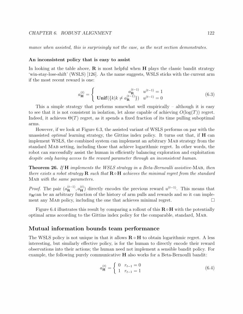
CHAPTER 6. ROBUST ALIGNMENT 122
mance when assisted, this is surprisingly not the case, as the next section demonstrates.
An inconsistent policy that is easy to assist
In looking at the table above, R is most helpful when H plays the classic bandit strategy‘win-stay-lose-shift’ (WSLS) [126]. As the name suggests, WSLS sticks with the current armif the most recent reward is one:
a(t)H =
a
(t−1)R u(t−1) = 1
Unif(k|k 6= a(t−1)R ) u(t−1) = 0
(6.3)
This a simple strategy that performs somewhat well empirically – although it is easyto see that it is not consistent in isolation, let alone capable of achieving O(log(T )) regret.Indeed, it achieves Θ(T ) regret, as it spends a fixed fraction of its time pulling suboptimalarms.
However, if we look at Figure 6.3, the assisted variant of WSLS performs on par with theunassisted optimal learning strategy, the Gittins index policy. It turns out that, if H canimplement WSLS, the combined system can implement an arbitrary Mab strategy from thestandard Mab setting, including those that achieve logarithmic regret. In other words, therobot can successfully assist the human in efficiently balancing exploration and exploitationdespite only having access to the reward parameter through an inconsistent human.
Theorem 26. If H implements the WSLS strategy in a Beta-Bernoulli assistive-Mab, thenthere exists a robot strategy R such that RH achieves the minimal regret from the standardMab with the same parameters.
Proof. The pair (a(t−1)R , a
(t)H ) directly encodes the previous reward u(t−1). This means that
πRcan be an arbitrary function of the history of arm pulls and rewards and so it can imple-ment any Mab policy, including the one that achieves minimal regret.
Figure 6.4 illustrates this result by comparing a rollout of this RH with the potentiallyoptimal arms according to the Gittins index policy for the comparable, standard, Mab.
Mutual information bounds team performance
The WSLS policy is not unique in that it allows R H to obtain logarithmic regret. A lessinteresting, but similarly effective policy, is for the human to directly encode their rewardobservations into their actions; the human need not implement a sensible bandit policy. Forexample, the following purely communicative H also works for a Beta-Bernoulli bandit:
a(t)H =
0 rt−1 = 01 rt−1 = 1
(6.4)

CHAPTER 6. ROBUST ALIGNMENT 123
We can generalize the results regarding communicative policies using the notion of mutualinformation, which quantifies the amount of information obtained through observing thehuman arm pulls.
Let I(X;Y ) be the mutual information between X and Y , H(X) be the entropy of X,and H(X|Y ) be the entropy of X given Y .
Theorem 27. Suppose that the probability the robot pulls a suboptimal arm at time t isbounded above by some function f(t), that is P (R(t) 6= j∗) ≤ f(t). Then the mutual infor-
mation I(j∗; a(1)H × · · · × a
(t)H ) between the human actions up to time t and the optimal arm
must be at least (1− f(t)) logK − 1.
Proof. We can consider the multi-armed bandit task as one of deducing the best arm fromthe human’s actions. This allows us to apply Fano’s inequality [41] to P (R(t) 6= j∗), andusing the fact that the entropy of a Bernoulli random variable is bounded above by 1, weget
P (R(t) 6= j∗) log(K − 1) ≥ H(j∗|j∗)− log 2
= H(j∗)− I(j∗; j∗)− 1
≥ logK − I(j∗; a(1)H × · · · × a
(t)H )− 1.
Rearranging terms and using P (R(t) 6= j∗) ≤ f(t), we get
I(j∗; a(1)H × · · · × a
(t)H ) ≥ logK − f(t) log(K − 1)− 1
≥ (1− f(t)) logK − 1.
Intuitively, since the probability of error is bounded by f(t), in (1−f(t)) cases the humanactions conveyed enough information for A to successfully choose the best action out of Noptions. This corresponds to logN bits, so there needs to be at least (1− f(t)) logN bits ofinformation in H’s actions.
Corollary 27.1. Suppose that the probability the robot pulls a suboptimal arm at time tis bounded above by some function f(t), that is P (R(t) 6= j∗) ≤ f(t). Then the mutual
information I(a(1)R × u(1) × · · · × a(t−1)
R × u(t−1); a(1)H × · · · × a
(t)H ) between the human actions
up to time t and the human observations must be at least (1− f(t)) logK − 1.
Proof. Since the best arm is independent of the human actions given the human observations,this follows immediately from the data processing inequality and proposition 27.
In order to achieve regret logarithmic in time, we must have that P (Kt 6= j∗) ≤ Ct
forsome C > 0. Applying proposition 27 above implies that we must have
I(j∗; a(1)H × · · · × a
(t)H ) ≥ (1− C
t) logK − 1

CHAPTER 6. ROBUST ALIGNMENT 124
...
...
3
3
rt 1 0 1 1
1
3
0 1
3
13
3
10
...
...
3 0, 1, 2 2
1
2 2 2, 3 3 3
H
A
R assumes H is learning
Gittins index
3
2
1
3
3
3
2 2 2
2 2 2
1
3
3
3
3
3
1
3
Figure 6.4: In Theorem 26 we show that it is possible to match the regret from optimallearning in an standard MAB when assisting the ‘win-stay-lose-shift’ (WSLS) policy. Thisis because WSLS perfectly communicates the observed rewards to R. Here we show anexample trajectory from an approximately optimal policy assisting WSLS. At the top is whatH suggests, followed by what R pulls, followed by the reward H observes. For comparison,we show the arms selected by the near-optimal Gittins index policy for each belief state.This highlights the importance of communicative learning policies in an assistive-Mab.
Note that the term I(j∗; a(1)H × · · · × a
(t)H ) depends on both the human policy and the
robot policy - no learning human policy can achieve this bound unless the human-robotsystem R H samples each arm sufficiently often. As a consequence, simple strategies suchas inferring the best arm at each timestep and pulling it, cannot achieve the Θ(log T ) lowerbound on regret. Our WSLS results agree with Theorem 26. Assisted WSLS achieves aregret of 3.5, close to the regret of the best-performing unassisted policy, 3.2. The gap inreward is due to our choice to employ approximate policy optimization. Qualitative analysisof WSLS trajectories found that it would often switch from its current arm after only asingle observation of failure, although this is clearly sub-optimal. We provide an exampletrajectory in Figure 6.4. The actions selected are almost identical to those of the optimalpolicy. This suboptimality also accounted for the small increase in regret when assisting theGittins index policy in Figure 6.3.
Theorem 27 implies that high mutual information is required for good team performance.To verify this, we computed the mutual information for a variety of combined policies after5 timesteps. Figure 6.5 plots this against the regret of the combined system. We considerseveral variants of ε-greedy and TS that are more or less deterministic. We consider ε ∈[0, 0.02, 0.05, 0.1]. To make TS more deterministic, we use the mean of a sample of n particlesto select arms. We consider n ∈ [1, 2, 3, 10, 30,∞].
Across this data, higher mutual information is associated with lower assisted regret,r(10) = −.82, p < .001. Furthermore, by looking at the ε-greedy and TS results as asequence, we can observe a clear and distinct pattern. Policies that are more deterministictend to be easier to help. This is supported by the results in Table 6.1, which shows that it

CHAPTER 6. ROBUST ALIGNMENT 125
0.10 0.15 0.20 0.25 0.30Mutual Information with best arm after 5 Timesteps (bits)
3.5
4.0
4.5
5.0
Reg
retw
ith
robo
tass
ista
nce
Assisted Regret vs Mutual Information
ε-GreedyWSLSThompson SamplingGittins Index
More random←− −→More deterministic
Figure 6.5: The assisted regret of various policies, plotted against the mutual informationbetween the best arm and the policy’s actions in the first 5 timesteps. We also plot thebest-fit line, with 95% confidence interval, for the regression between assisted regret andmutual information. We augmented our policies with variants of ε-greedy and Thompsonsampling with less randomness. Policies with high mutual information lead to lower regretwhen assisted, supporting our theoretical findings.
is easier to infer reward parameters for WSLS and GI (i.e., the two policies with the highestmutual information) than TS and ε-greedy.
The assistive multi-armed bandit considered so far only captures one mode of interaction.It is straightforward to consider extensions to different modes. We consider two such modes.The first is turn taking, where H and R take turns selecting arms. This can be more difficultbecause the robot has to act in early rounds, when it has less information, and because thehuman has to act in later rounds, when H may be noisy and the best arm has already beenidentified.
The second variant we consider is preemptive interaction. In this case, R goes first andeither pulls an arm or lets H act. This creates an exploration-exploitation tradeoff. R onlyobserves H’s arm pulls by actually allowing H to pull arms and so it must choose betweenobserving H’s behavior and exploiting that knowledge.
Figure 6.6 compares the performance of different assumptions about H for both of theseinteraction modes. The results are largely similar to those of the original model. We are
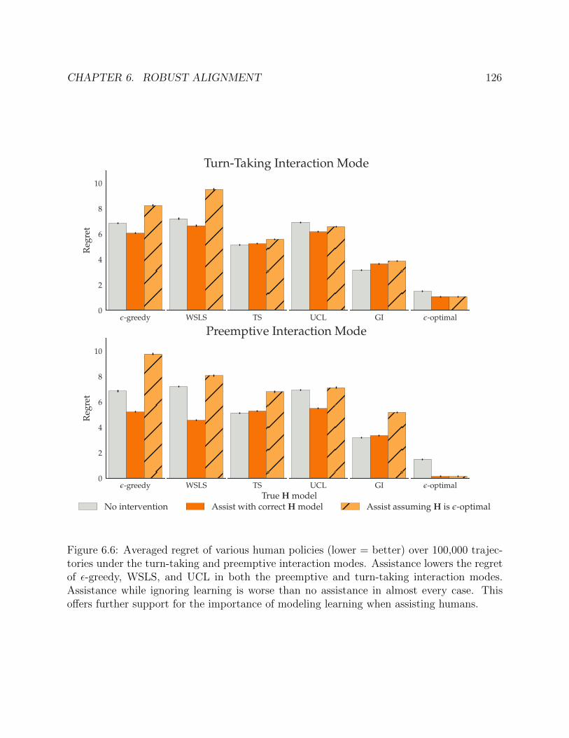
CHAPTER 6. ROBUST ALIGNMENT 126
ε-greedy0
2
4
6
8
10
Reg
ret
ε-greedy0
2
4
6
8
10
Reg
ret
WSLS
WSLS
TS
Turn-Taking Interaction Mode
TS
Preemptive Interaction ModeUCL
UCL
GI
GI
ε-optimal
ε-optimal
No intervention Assist with correct H model Assist assuming H is ε-optimalTrue H model
Figure 6.6: Averaged regret of various human policies (lower = better) over 100,000 trajec-tories under the turn-taking and preemptive interaction modes. Assistance lowers the regretof ε-greedy, WSLS, and UCL in both the preemptive and turn-taking interaction modes.Assistance while ignoring learning is worse than no assistance in almost every case. Thisoffers further support for the importance of modeling learning when assisting humans.
CHAPTER 6. ROBUST ALIGNMENT 127
able to assist the suboptimal policies and modeling learning as ε-optimality increases regretin all cases. We obtain results that confirm Theorem 27: more deterministic policies thatreveal more information are easier to help.
Additionally, we see that WSLS is a less attractive policy in these settings: becauseH actions are always executed when they are observed, it no longer makes sense for H toemploy a purely communicative policy. However, because actions have an effect on utilitydirectly (i.e., H actually interacts with the world, rather than only providing information toR) this breaks the symmetry between ‘win-stay-lose-shift’ and ‘win-shift-lose-stay.’ Thus,this loss in utility is compensated for by ruling out a perverse outcome where H and R usestrategies from mismatched pedagogical equilibria in a way that causes R H to minimizeutility.
Explore, observe, then exploit
In looking at the policies learned for the preemptive interaction mode, we see an interest-ing pattern emerge. Because the policy has to choose between selecting arms directly andobserving H, by looking at rollouts of the learned policy we can determine when it is mostuseful to observe H. We find that a clear pattern emerges. R initially explores for H: itselects arms uniformly to give H a good estimate of θ. Then, R observes H’s arm pullsto identify the optimal arm. For the final rounds, R exploits this information and pulls itsestimate of the optimal arm. Figure 6.7 compares a representative trajectory with one thatis optimized against an ε-optimal H.

CHAPTER 6. ROBUST ALIGNMENT 128
H is -Optimal
exploitobserve
defer
...
... rt 1 1 0 1 1 1
H
A
H is -Greedy
rt
...
...
0
1 2
...
...3
1 10 1 1 0 1
explore exploitobserve
H
A
3
33
3
33 3
333
deferdefer
1
defer defer defer
R
R
Figure 6.7: A comparison between assisting an ε-optimal H and an ε-greedy H in a modifiedassistive-Mab where the robot R has to choose between acting and letting H act. Thiscreates a direct exploration-exploitation tradeoff that makes it easier to qualitatively analyzeR’s behavior. At the top is whether R defers to the human or pulls an arm, followed bywhat H pulls (if the robot defers), followed by the reward H observes. When the robotmodels learning, the policy it learns has a qualitative divide into three components: explore,where the robot explores for the human; observe, when the robot lets the human pull arms;and exploit, when the robot exploits this information and pulls its estimate of the best arm.Crucially, the explore component is only found when learning is modeled. This illustratesTheorem 25, which argues that assisting an ε-optimal H is different from assisting a learningH.

129
Chapter 7
Related Work
In this chapter we collect work related to the analysis of the principal—agent value alignmentproblem in artificial intelligence.
7.1 The Economics of Principal–Agent Relationships
and Incomplete Contracting
In Chapter 1, we discussed how the development of computational methods to select optimalactions for a given set of incentives was a crucial step in the development of AI systems. Asa result, incentive alignment issues for artificial agents have clear analogues in the humanprincipal–agent problem long studied by economists and legal scholars. Kerr [85] providedan early description of a wide variety of misaligned incentives in the aptly titled “On the follyof rewarding A, while hoping for B.” Gibbons [51] provides a useful survey of principal–agentmodels and their applications.
Reasons for incompleteness
As discussed in Chapter 1, the principal–agent problem in economics is studied as a problemof optimal contracting. In this theory, contracts specify payments and allocation of resourcesto the contracting parties in different states of the world. This is analogous to the rewardfunction or objective used to specify autonomous behavior in AI approaches. A completecontingent contract specifies these incentives for every possible world state that can bereached. If complete contingent contracts were possible, perfect alignment between principaland agent would be possible. However, it is understood that contracts are routinely, andlikely unavoidably, incomplete. Economists have identified multiple reasons for contractualincompleteness:
• unintended incompleteness: contract designers fail to identify all circumstances thataffect the value of the contract. This is sometimes referred to as bounded rationality

CHAPTER 7. RELATED WORK 130
[145, 175].
• economizing on costly cognition and drafting: contract designers choose not to investin the costly cognitive effort of discovering, evaluating and drafting contract terms tocover all circumstances [141, 142, 137].
• economizing on enforcement costs: contract designers leave out terms that are costlyto enforce because they require more or more costly evidence or because the potentialfor disputes and/or court errors increases with the complexity of the contract [86, 136,74].
• non-contractibility: some contingencies and/or actions are left out because either theycannot be observed or, even if observable, they cannot be verified by enforcers atreasonable cost. This might be because of hidden information or it might be becauseit is not possible to communicate (describe) the contingency or action in unambiguousterms [63, 107].
Contractual incompleteness is typically framed as undesirable. In most of the settings con-sidered in this work, this is the case. In Section 3.2, for example, H’s inability to specifya complete representation of preferences led to lost utility. In addition to that, economistshave also considered settings in which completeness is feasible but not optimal. These arecases in which information at the time of contracting is incomplete and new information isanticipated in the future:
• planned renegotiation: rather than writing a complete contract based on incompleteinformation at the start of a contracting relationship, contract designers choose towrite an incomplete contract, which they expect to renegotiate in the future once moreinformation becomes available [19, 74]
• optimal completion of contract by third-party: rather than writing a complete contractbased on incomplete information at the start of a contracting relationship, contractdesigners choose to write an incomplete contract, which they expect to have filled inby a third-party adjudicator with better information in the future [66, 142]
In this work, we can view the dynamic incentives protocol from Section 4.3 as an exampleof planned renegotiation. By designing an agent to limit the scope of the initial incentives,and update them in response to the observation of a new environment, the team is ableto efficiently manage the transfer of normative information (i.e., information about how toevaluate different states of the world) from H to R.
This is not a perfect analogy because there exists a complete specification of rewardswhich would work across all environments. The assistive-Mab introduced in Section 6.2 isa better model of a scenario where a complete contract would be suboptimal. H does notknow how to evaluate the different options at the start of the game, and so it would be

CHAPTER 7. RELATED WORK 131
suboptimal to specify complete incentives for which arm R pulls. Instead, H does best whenthey are able to update R’s incentives in response to reward observations made over time.
As a final category of incomplete contracts, economists, and many legal scholars, haveidentified strategic behavior as another reason for incompleteness:
• strategic protection of private information: a party with private information abouta missing contingency does not prompt contracting to cover the contingency becausedoing so will reveal private information that reduces the value of the contract [155, 12]
• deterring strategic investments in costly cognition : the parties choose not to coverall contingencies because learning about them would be biased and wasteful, partlymotivated by efforts to protect against strategic wealth transfers that will occur if thecontingency arises [167]
• strategic ambiguity:the parties choose not to include all known and contractible con-tingencies in order to control strategic behavior in response to other noncontractiblecontingencies [17]
This class of reasons for incompleteness does not translate as readily to the principal–agent problems considered in this work. The models considered for this dissertation havefocused on a dyadic relationship between a system designer and a robot. In dyadic rela-tionships between people, strategic incentives typically arise from the fact that people, ingeneral, have different goals. In contrast, an autonomous agent’s preferences are much moreof a blank slate. However, it is easy to see that these strategic concerns will arise if weconsider interactions with more than one person. Consider, e.g., a model with 2 humans, asystem designer and a system user. The divergence of the two human’s objectives will createincentives for the human to strategically conceal information about their preferences thatcould be used against them in the future. To analyze these questions, future work shoulddraw upon the implications of mechanism design [112] research as it applies to the design ofcomplex autonomous systems. Fickinger et al. [44] describes an initial analysis in this settingand shows that, if the human players are directly rewarded for a large enough fraction oftheir action, it is possible to circumvent several negative results from voting theory.
Multitask models and distorted incentives
One of the central results from the study of incomplete contracting is the observation that thestructure of the optimal incomplete contract should take that incompleteness into account.A well-studied example of this is the case of multitask principal–agent problems, where aagent must divide its effort across a variety of distinct tasks.
Holmstrom and Milgrom [78] and Baker, Gibbons, and Murphy [13] show that the optimalincentive contract for a task that can be measured should take into account the impact ofthose rewards on effort put towards tasks that cannot be measured. In particular, it may bebetter to reduce the quality of incentives on the measurable task below what is feasible, in

CHAPTER 7. RELATED WORK 132
order to reduce the distortion introduced in the unmeasurable task. The model of incompleteproxy metrics from Section 3.2 can be seen as an extreme example of this, where some taskscan be measured perfectly while others can not be measured at all.
Holmstrom and Milgrom [78] gives the example of paying a teacher a fixed salary ratherthan one contingent on students’ (easily measurable) standardized test scores. At first glance,it seems like the latter approach would be a good way to leverage incentives to improvelearning outcomes. However, overly strong incentives leads to the phenomenon of “teachingto the test,” where teachers dedicate too much classroom time to specific test preparationactivities (e.g., process of elimination methods for multiple choice questions). This leads toless time spent on difficult-to-measure skills like creative problem solving and, in effect, thetest becomes uncorrelated from these learning goals.
Baker, Gibbons, and Murphy [13] gives the example of an auto repair shop rewardingmechanics for completed repairs and thereby inducing mechanics to mislead customers aboutthe need for repairs: completion of repairs is easily measurable; the reliability of a mechanic’sdiagnosis of car problems is not. More generally, sometimes it is better for a contract not toinclude easily contractible actions in order not to further distort incentives with respect tonon-contractible actions.
When we consider the role of distorted incentives in the design of AI systems, we canobserve a key difference between an artificial agent and a human one. In the absence ofexplicit incentives from the contract, a human will fill in the gaps with nuanced and intelligentinterpretation. While this might not be desirable from the perspective of managing strategicbehavior, the ability to draw on commonsense interpretations is incredibly valuable.
Contracts do not exist in a vacuum; they come heavily embedded in social and insti-tutions structures [61]. At a minimum, they depend on shared language and organizedstructures for enforcement: formal enforcement through courts and coercive authorities andinformal enforcement through social sanctions such as collective (coordinated) criticism andexclusion from valuable relationships. Incomplete contracts depend even more extensively onthese external, third-party institutions: not only to enforce contractual terms but to supplycontractual terms by interpreting ambiguous terms and filling in gaps. They contain notonly their express terms but also their interpreted and implied terms [42]. This importantpoint has been emphasized by legal scholars, in a field known as relational contracting, forseveral decades [99, 102, 101, 103, 55].
In the design of AI systems, it is crucial to develop methods that imitate, in general,this reliance on, and sensitivity to, external normative structure. This could include explicitmechanisms for an AI agent’s objective to reference externally defined or controlled metricsor research into the cognitive processes that set these incentives for people. This conceptoverlaps with the economist’s definition of relational contracting (see [52] for a review) tothe extent that it focuses on informal sanctions for breach of obligations. Legal scholars inthe sociological tradition have always included here a wide variety of sanctions (includinginternalized sanctions such as guilt and shame). Economists, on the other hand, typicallyhave modeled the termination of valuable economic relationships or the degradation of rep-utation, which reduces contracting opportunities with third-parties in the future. The legal

CHAPTER 7. RELATED WORK 133
concept of relational contracts goes further than enforcement to focus also on the impor-tation of obligations into a contractual relationships from sources other than the expresslanguage of an agreement. Williamson [175], Alchian and Demsetz [6] and Klein, Crawford,and Alchian [87] were the first economic treatments to focus on this aspect of the legalanalysis of relational contracts.
7.2 Impact Minimization
In Section 3.3, we identify two potential strategies to avoid the negative results about guar-anteed overoptimization of proxy metrics: impact minimization methods and dynamic in-centives protocols. While dynamic incentives have received less academic attention, severalpapers have considered generic proposals for impact measurement and penalization.
Armstrong and Levinstein [11] proposes the inclusion of a large impact penalty in the AIagent’s utility function. In this work, they suggest impact be measured as the divergencebetween a distribution of states of the world and the distribution if the AI agent had notexisted. Thus, distributions sufficiently different would be avoided. Alternatively, otherapproaches use an impact regularizer learned from demonstration instead of one explicitlygiven [9].
Krakovna et al. [92] expand on this work by comparing the performance of various im-plementations of impact minimization in an AI Safety Gridworld suite [97]. They proposea reachability condition which penalizes the system for removing the ability to navigate thesystem to states that were previously reachable. In doing so, the hope is that the systemwill avoid unrecoverable failures.
Turner, Hadfield-Menell, and Tadepalli [169] considers an analogous method where theagent is penalized for changes in a vector of value functions, where the value functions arecomputed based on a set of candidate reward functions. This forces the agent to accomplishits goal with minimal effect on the state of alternative tasks. Turner, Ratzlaff, and Tadepalli[168] shows that this method is effective at avoiding side-effects in an adaptation of Conway’s‘Game of Life’ [3].
Krakovna et al. [91] provides a theoretical grounding of these approaches in a settingwhere the agent must preserve the ability to perform future tasks. They formalize theproblem of interference, where the consideration of future tasks leads the agent to performtasks that are useful for the overall distribution of tasks and show how to modify the objectiveto remove this incentive. This approach is quite interesting in the context of the combinedtheoretical solution discussed at the end of Chapter 3: it defines a regularizer that explicitlyprevents R from interfering with the ability to maximize future (proxy) objectives. Thus,we can see this method, combined with the dynamic incentives protocol in Section 4.3 as aninteresting proposal for a value alignment solution based on proxy objectives.

CHAPTER 7. RELATED WORK 134
7.3 Inverse Reinforcement Learning
From a technical standpoint, the starting point for the analysis in this thesis resides in theframework of inverse reinforcement learning. Ng and Russell [115] define inverse reinforce-ment learning (Irl) as follows:
Given: 1) measurements of an agent’s behavior over time, in a variety of cir-cumstances, 2) if needed, measurements of the sensory inputs to that agent; 3)if available, a model of the environment.Determine the reward function being optimized.
In Section 2.3, we give an formulation of the problem. Here, we go over some of the keyresults in the area.
Ng and Russell [115] use a mathematical programming approach to characterize theset of potential Irl solutions for a given set of demonstrations. They identify one of thecentral challenges in Irl: for any demonstration, there are typically many reward functionsthat could be optimal. In the context of this dissertation, this essentially states that ademonstration of an optimal trajectory is an incomplete representation of H’s goal.
Abbeel and Ng [2] considered the problem of Irl with linear reward functions and showedthat a policy that matches the feature expectations from the demonstrations will always getthe same amount of reward as the expert. Ratliff, Bagnell, and Zinkevich [123] show howto use subgradients to efficiently compute weights that maximize the margin between thedemonstrations and alternative trajectories. Ramachadran and Amir [122] and Ziebart etal. [181] both considered the problem of learning reward functions from noisy behavior.Ramachadran and Amir [122] use Markov-chain Monte Carlo methods to compute an ap-proximate posterior over reward functions. The key idea in their approach is to combine aspecific proposal distribution of candidate rewards with a method for efficiently re-using thesolutions to previous reward functions.
Ziebart et al. [181] highlights the importance of modeling the details of the choice setconsidered by the demonstrator. They show the difference between a distribution of behaviorthat selects actions in proportion to the Q function and one that selects trajectories inaccordance with their total utility. While this is structurally similar, the difference hasto do with the way that noise accumulates. As an example, they consider an Mdp with 3trajectories, all of equal utility. They show that the policy which selects actions in proportionto their Q-value leads to an uneven distribution over trajectories cause by the environmentdynamics. They introduce a dynamic programming method to compute this distribution ontrajectories and use it to propose an effective gradient-based method for Irl.
Syed and Schapire [162] describes an adversarial approach to Irl and apprenticeshiplearning. They consider a setting where an adversary can select a reward function in orderto maximize the regret of a deployed policy. Interestingly, their method allows imitationto improve on demonstrator performance, depending on the structure of the deploymentdomain.

CHAPTER 7. RELATED WORK 135
A recent area of focus in Irl research is the development of methods that can scaleto nonlinear reward spaces like neural networks. Finn, Levine, and Abbeel [45] proposed amethod that uses policy learning instead of planning to deal with high-dimensional problems.Ho and Ermon [77] proposed an adversarial approach that uses a neural network trained todistinguish optimized and demonstrated trajectories to train an imitation policy. Fu, Luo,and Levine [48] learn state-only rewards with this approach and show that their method canlearn reward functions that are disentangled from the problem dynamics in the sense thatthey create incentives the optimal policy across a set of transition dynamics.
Natarajan et al. [113] introduce an extension to Irl where R observes multiple actorsthat cooperate to maximize a common reward function. This is a different type of coop-eration than we consider, as the reward function is common knowledge and R is a passiveobserver. Waugh, Ziebart, and Bagnell [172] and Kuleshov and Schrijvers [93] consider theproblem of inferring payoffs from observed behavior in a general (i.e., non-cooperative) gamegiven observed behavior. Combining these methods with the assistance game formulationsconsidered in this work is an interesting direction in which to study the problem of assistinggroups of humans with competing objectives.
7.4 Reward Learning
In addition to Irl there are a variety of methods for reward learning that have been studiedin artificial intelligence. There is a vast number of preference learning methods for non-sequential problems [49]. Methods that learn reward functions from preferences, surveyed inWirth, Furnkranz, and Neumann [176], are particularly relevant to our work.
Christiano et al. [34] learn a reward function from preferences over pairs of trajectories,by sampling trajectories from a learned policy and querying the user about pairs with highuncertainty. A similar setup is used in Wirth, Furnkranz, and Neumann [176] and Akrour,Schoenauer, and Sebag [5], based around other policy optimization methods. It is alsopossible to learn reward functions from preferences on actions [49] and states [128]. Many ofthese methods select from already encountered trajectories, which will be guesses at optimaltraining behavior. Sadigh et al. [130] identify queries by gradient-based optimization in thetrajectory space (in continuous environments).
Reward functions are also frequently learned from direct reward values [88, 171] andexpert ratings [35]. An interesting genre of this work looks at learning from trajectoryrankings, where an expert provides a total ordering over a set of possible comparisons.Brown et al. [24] give a promising approach that combines trajectory ranking to learn adistribution over reward functions that can be effectively maximized in a risk-averse fashionin novel environments. This is similar to the approach taken in Ird (where a proxy objectiveprovides a ranking over all trajectories in the development environment) but Brown et al.[24] are able to scale their method to much larger problems and more complex reward spaces.Their approach is notable for its simplicity: rankings are converted into pairwise preferencesand used to train a classifier.

CHAPTER 7. RELATED WORK 136
Shah et al. [138] argue that these reward learning approaches can be united by observingthat each models H’s choice as a reward-driven choice over different option sets. They cataloga wide variety of distinct reward feedback mechanisms and their associated probabilisticassumptions. In the context of this dissertation, these correspond to different choices of theaction spaces for H AH and/or different choices of H’s policy πH.
Shah et al. [139] takes an interesting approach to reward learning that relies on the initialstate of the world. The core idea is that the initial state that a robot is deployed into is rarelya truly ‘random’ draw from a distribution. Instead, it is often heavily optimized towardsdifferent (human) objectives. The key idea in this paper is that by considering the initialstate as an optimized environment, it is possible to learn about the objectives that statewas optimized towards. Crucially, this justifies the deployment of low-impact policies. In ageneral state of nature, there is no reason to minimize impact.
Shaikh and Goodrich [140] proposes and evaluates several interfaces for reward specifi-cation, eliciting three-way trade-offs from users. This is complementary to Ird, and couldbe adapted to collect data for our method. Furthermore, the divide-and-conquer strategysuggests a natural way to scale this approach to collect arbitrary n-way trade-offs becausewe can combine observations from several three-way interactions.
7.5 Optimal Reward Design
Singh et al. [148] formalize and study the problem of designing optimal rewards. Theyconsider a designer faced with a distribution of environments, a class of reward functionsto give to an agent, and a fitness function. They observe that, in the case of boundedagents, it may be optimal to select a proxy reward that is distinct from the fitness function.Sorg, Singh, and Lewis [154] and subsequent work has studied the computational problemof selecting an optimal proxy reward.
In Section 4.2, we considered an alternative situation where the system designer is thebounded agent. In this case, the proxy reward function is distinct from the fitness function– the true utility function in our terminology – because system designers can make mistakes.Ird formalizes the problem of determining a true utility function given an observed proxyreward function. This enables us to design agents that are robust to misspecifications intheir reward function.
MacGlashan et al. [100] presents a system to ground natural language commands toreward functions that capture a desired task. Using natural language as an interface forspecifying rewards is complementary to our approach as well.
7.6 Pragmatics
The pragmatic interpretation of language is the interpretation of a phrase or utterance inthe context of alternatives [62]. For example, the utterance “some of the apples are red” is
CHAPTER 7. RELATED WORK 137
often interpreted to mean that “not all of the apples are red” although this is not literallyimplied. This is because, in context, we typically assume that a speaker who meant tosay “all the apples are red” would simply say so. Recent models of pragmatic languageinterpretation use two levels of Bayesian reasoning [47, 60]. At the lowest level, there isa literal listener that interprets language according to a shared literal definition of wordsor utterances. Then, a speaker selects words in order to convey a particular meaning tothe literal listener. To model pragmatic inference, we consider the probable meaning of agiven utterance from this speaker. We can think of inverse reward design from Chapter 4as a model of pragmatic reward interpretation: the speaker in pragmatic interpretation oflanguage is directly analogous to the reward designer in Cirl.
7.7 Corrigible Systems
Omohundro [117] identifies the instrumental goals of artificial agents: goals which are likelyto be adopted as subgoals of most objectives. He identifies an incentive for self-preservationas one of these instrumental goals. Soares et al. [151] takes an initial step at formalizingthese arguments. They refer to agents that allow themselves to be switched off as corrigibleagents. They show that one way to create corrigible agents is to make them indifferent tobeing switched off, but in their model this also makes R equally likely to commit suicideas to take any other action. The key difference in our formulation in Section 4.1 is thatR knows that it does not know the utility function U . This gives a natural way to createincentives to be corrigible and to analyze the behavior if R is incorrigible.
Orseau and Armstrong [119] consider the impact of human interference on the learningprocess. The key to their approach is that they model the off-switch for their agent as aninterruption that forces the agent to change its policy. They show that this modification,along with some constraints on how often interruptions occur, allows off-policy methods tolearn the optimal policy for the given reward function just as if there had been no interference.Their results are complementary to ours. In Section 4.1, we determine situations where theoptimal policy allows the human to turn the agent off, while they analyze conditions underwhich turning the agent off does not interfere with learning the optimal policy. We haveshown that R’s obedience depends on a tradeoff between R’s uncertainty about and H’srationality. However, they considered R’s uncertainty in the abstract. In practice R wouldneed to learn about utility evaluations through H’s behavior. Our work analyzes how theway R learns about reward impacts its performance and obedience.
7.8 Intent Inference For Assistance
Instead of just being blindly obedient, an autonomous system can infer H’s intention andactively assist H in achieving it. We formalize this problem as a supervision-PoMdp inSection 3.1. ‘Do What I Mean’ software packages interpret the intent behind what a pro-

CHAPTER 7. RELATED WORK 138
grammer wrote to automatically correct programming errors [164]. When a user uses atelepointer network lag can cause jitter in their cursor’s path. Gutwin, Dyck, and Burkitt[65] address this by displaying a prediction of the user’s desired path, rather than the actualcursor path.
Similarly, in assistive teleoperation, the robot does not directly execute H’s (potentiallynoisy) input. It instead acts based on an inference of H’s intent. In Dragan and Srinivasa[39] R acts according to an arbitration between H’s policy and R’s prediction of H’s policy.Like our work, Javdani, Bagnell, and Srinivasa [80] formalize assistive teleoperation as aPoMdp in which H’s goals are unknown, and try to optimize an inference of H’s goal.
7.9 Cooperative Agents
Fern et al. [43] consider a hidden-goal Mdp, a special case of a PoMdp where the goal isan unobserved part of the state. This is similar to the assistance-PoMdp model introducedin Chapter 4, where the set of possible objectives are binary functions of the goal state.The frameworks share the idea that R helps H accomplish a partially observed objective.The key difference between this model and the Cirl model considered in Chapter 5 lies inthe treatment of the human (the agent in their terminology). In Cirl, we treat H as anactor in a decision problem that both actors collectively solve. This allows us to analyzethe problem for robustness with respect to the human policy and is crucial to modeling thehuman’s incentive to teach.
Woodward, Finn, and Hausman [177] considers the problem of training assistive agent asa meta-learning problem. They propose a policy learning approach that is able to identifyeffective teaching and learning policies for H and R. The primary extension beyond Cirlmethods is that they consider a setting with partial observability for both H and R.
Carroll et al. [28] considers the problem of learning teamwork behaviors via self-play.Their work identifies the substantial coordination challenges that arise from multiple parallelequilibria. Unlike in adversarial settings, where an opponent that performs suboptimallytypically helps the performance of a strategy, it will typically hurt a cooperative behavior.They show, via a user study, evidence of pedagogical behavior from their subjects that cancounteract R’s mistake over time and H gets a better model of πR. This indicates theimportance of studying adaptive solutions to cooperative decision problems.
Boutilier [22] introduces the problem of multiagent-Mdps, which formalizes these co-ordination problems. Boutilier proposes a simple solution that augments an Mdp with acoordination state in situations where there are multiple potentially optimal actions. Thisallows agents to learn to coordinate online via a simple, randomized coordination mecha-nism. Wu et al. [178] propose a method that uses a hierarchical model to infer subgoals thatagent’s have selected online to allow for a more scalable form of this adaptive planning. Thisclass of problem has also been studied in the context of ad-hoc teamwork, which proposesmethods for evaluating the performance of agents in a setting where coordination is notpossible beforehand.

CHAPTER 7. RELATED WORK 139
7.10 Optimal Teaching
Because Cirl creates incentives for the human to teach, as opposed to maximizing rewardin isolation, our work is related to optimal teaching: finding examples that optimally traina learner [14, 57, 56]. The key difference is that efficient learning is the objective of optimalteaching, while it emerges as a property of pedagogical equilibrium in Cirl.
Cakmak and Lopes [25] consider an application of optimal teaching where the goal is toteach the learner the reward function for an Mdp. The teacher gets to pick initial states fromwhich an expert executes the reward-maximizing trajectory. The learner uses Irl to infer thereward function, and the teacher picks initial states to minimize the learner’s uncertainty. InCirl, this approach can be characterized as an approximate algorithm for H that greedilyminimizes the entropy of R’s belief.
Beyond teaching, several models focus on taking actions that convey some underlyingstate, not necessarily a reward function. Examples include finding a motion that best com-municates an agent’s intention [38], or finding a natural language utterance that best com-municates a particular grounding [58]. All of these approaches model the observer’s inferenceprocess and compute actions (motion or speech) that maximize the probability an observerinfers the correct hypothesis or goal. Our approximate solution to pedagogical demonstra-tion in Section 5.1 is analogous to these approaches, in that we compute actions that areinformative of the correct reward function.
7.11 Algorithms for Planning with Partial
Observability
Algorithms for Mixed-Observability Decision Problems
The supervision-PoMdp and assistance-PoMdp formulations we consider in this work areexamples of mixed-observability Markov decision process (Momdp) since the state space canbe factored into a fully and a partially-observable component. This structure allows for moreefficient solution methods. Ong et al. [118] leverage the factored nature of the state spaceto create a lower dimensional representation of belief space. This core idea is orthogonalto ours, which exploits Cirl’s information asymmetry instead. The two can be leveragedtogether.
Partially-observable Markov decision processes
We chose to explicate our modified Bellman update from Section 5.2 in the context of PBVIand POMCP because they are the seminal point-based and MCTS algorithms respectively,for solving POMDPs. For example, SARSOP [94] and DESPOT [152], two state-of-the-artalgorithm for POMDPs, are variants of PBVI and POMCP respectively. The principles weoutlined in Section 5.2 and can be easily adapted to a large variety of point-based and MCTS
CHAPTER 7. RELATED WORK 140
algorithms, including any which may be developed in the future, to derive even more efficientalgorithms for solving Cirl games.
Decentralized POMDPs
Dec-PoMdp algorithms can be used to compute pedagogical equilibria for Cirl gamesdirectly, without using the PoMdp reduction. Oliehoek and Amato [116] provides a usefulintroduction to the topic and an overview of solution methods. While exact solution methodsare generally intractable for any but the smallest problems, recent work has made progresson this front. Such Dec-PoMdp algorithms which attempt to prune away unreasonablestrategies resemble our approach. Amato, Dibangoye, and Zilberstein [7] use reachabilityanalysis to identify reachable states, then consider all policies which are useful at such states.
Hansen, Bernstein, and Zilberstein [75] model other agents possible strategies as partof a players belief, and prune away weakly dominated strategies at each step. While suchapproaches use heuristics to prune away some suboptimal strategies, we leverage the in-formation structure of Cirl to compute the optimal strategy for H and prune away allother strategies. This guarantees an exponential reduction in complexity while preservingoptimality; this is not true for the other methods.

141
Chapter 8
Directions for Future Work
My long-term research goal is to ensure that AI systems are effective in carrying out thegoals of their users and designers, despite fundamental limitations on our ability to specifythose goals. This dissertation introduces a simple formulation for the assistance game anddeveloped theory and algorithms therein. This chapter describes a research agenda thatbuilds on these results with a focus on scaling algorithms to work in complex robotics envi-ronments, developing a theory of reward learning to focus on minimizing misalignment, andextending the theory of value alignment to the case of multiple principals or value systems.
Accounting for more complex models of human (ir)rationality
The work in this dissertation has focused on principal–agent settings where the human playeris modelled as behaving optimally or approximately optimally. An important next step inthis research program is to consider the impact of more realistic cognitive or informationallimits on the human player’s strategy. Section 6.2 describes initial work in this direction: weconsider the impact of a human player that is learning about her objectives over time. Wediscuss what it means to meaningfully assist such an agent and identify broad conditionsin which assistance is possible. In the future, I intend to investigate the impact of similarrestrictions to account for limited memory, planning ability, or information about the world.Additionally, it is important to consider the impact of changing preferences, individual in-consistency, and variations in values across different people and groups. This will allow usto understand the theoretical limits of robot assistance and identify minimal criteria for theprincipal’s knowledge of and ability to communicate their objectives so that value alignmentis well-defined and feasible.
An integrated design environment for behavior
We currently rely on an AI system designer to directly specify loss functions, environments,and policy space in general purpose programming languages. This requires a huge amountof knowledge and often produces brittle learning systems. Developments such as AutoML

CHAPTER 8. DIRECTIONS FOR FUTURE WORK 142
simplify the design process and reduce the design effort for AI systems. However, theyalso make the system more reliant on the loss function selected and data provided, placingan increased burden on the designer to supervise and verify performance. To ensure thatthese systems perform reliably at scale, we need to design specification methods that 1) canscale to the complexity of modern AI datasets and problems; 2) can scale to the complexityof human preferences; and 3) naturally integrate oversight and verification. This researchprogram essentially reduces the problem of designing AI systems to a human-computer inter-action problem where optimization and reward learning compile the high-level language ofpreferences into executable behaviors. Designing AI systems in this fashion, combined withprogress on other robotics challenges such as uncertainty in perceptual systems and motorcontrol, allows us to optimize for more complex decisions, naturally integrate oversight andsupervision, due to the tight relationship between oversight and training, and use learningto inform the design process and reduce overall designer effort.
Loss functions for reward learning
The analysis of the off-switch game and inverse reward design in Chapter 4 shows that AIsystems should model (or at least adapt to) uncertainty in reward learning, in additionto more traditional types of uncertainty about state, dynamics, and controls. The nextnext question is, what properties of the robot’s reward model lead to better performance?There are clear ways that learning a reward function that will be optimized later is a differentlearning problem from standard supervised ranking or classification. In future research, I willdevelop a theory of learned reward functions that can explain this difference. For example,perhaps there is an appropriate regularizer for ranking functions that reduces overall riskfor planning. Another area to explore is learning objectives that naturally encode the riskaversion implemented with the Bayesian approach of inverse reward design. Similarly, anasymmetric loss function that penalizes predicting rewards that are too high more thanrewards that are too low could help with the stability of optimized policies for learnedrewards. The goal of this research is to understand the problem of learning incentives froma theoretical perspective and design reward learning methods that are naturally risk-averseand scale up to larger problems than state-of-the-art Bayesian inference can handle.
Value alignment with multiple principals.
In addition to continued work on the algorithmic and theoretical foundations of single-humansingle-robot value alignment, the research described in this dissertation can be extended toconsider value alignment in the context of multiple principals: multiple people with dif-ferent values and goals on whose behalf a system is supposed to take action. This posesa host of interesting algorithmic questions (e.g., scaling up to a large number of people),theoretical questions (e.g., what are the limits of computational social choice theory), andethical questions (e.g., how should we handle conflicts of values within AI systems; what arethe obligations of system designers to design systems that optimize for their users’ benefit).

CHAPTER 8. DIRECTIONS FOR FUTURE WORK 143
Solving a multiple-principal value-alignment problem can also involve modeling the interac-tions between a regulator, a company, and its AI agent. We can consider the optimal wayto provide incentives for companies to, e.g., invest in oversight and safety research.
AI regulation
In the limit of many principals, the value-alignment problem is closely related to the reg-ulation of AI systems. It formalizes the problem of designing systems that implement thevalues of collections of humans (contracting parties, organizations, cities, states, and soon). An example of this type of work is the development of procedures for human over-sight of AI decision-making systems. Work on explainable AI attempts to provide human-understandable accounts of why a complex and opaque AI system behaves as it does. Theanalysis in this dissertation calls for focusing instead on what I call justifiable AI: providingreasons for machine decisions that are acceptable to the people they impact. While this doesnot directly solve the problem of balancing competing goals between people, it will allowAI systems to be subject to the normative infrastructure that exists to regulate decisionsmade by people. In ongoing work with colleagues, our goal is to develop a procedure thatensures that organizations (corporations, health care systems, governments, etc.) that de-ploy AI-based decision making systems can verify that their systems are both a) sufficientlypredictable by humans and b) only make decisions that can be adequately justified by aspecified principal. This creates the conditions needed to hold a person meaningfully re-sponsible for an AI system’s behavior. Thus, aligning an AI system with that principal willcreate incentives for the system to abide by existing regulations and laws.
Interactive embodied value alignment for a home assistant
A crucial and ubiquitous principal–agent relationship is the relationship between a homerobot and its user or users. This challenge integrates the problem of scale (coordinating adiverse set of actions in a large state space over a long horizon), exploration/exploitationtradeoffs in online preference learning, and issues of value conflict among humans (e.g., dis-agreement over the thermostat). Furthermore, it will spur the development of methods thatcan account for these complexities in conjunction with issues around long-horizon planning,noisy sensors, and high-dimensional motor control. A value-alignment approach to the designof such a system allows the system to learn from multi-modal data about preferences andnaturally allows for the management of uncertainty about those preferences. Such researchdraws on hierarchical planning [68, 32, 72], planning under uncertainty [71] and manipulationplanning [69, 96].
Value alignment for content recommendation
The focus in this dissertation on value alignment is guided by a commitment to ensure thatAI is developed in ways that are safe and beneficial for society. A specific research applica-

CHAPTER 8. DIRECTIONS FOR FUTURE WORK 144
tion is the theory, design, and regulation of value-aligned content recommendation systems.These heavily optimized systems are widely deployed and are showing significant negativeexternalities such as addictive behaviors in young people, the spread of disinformation andconspiracy theories, and undermining the integrity of elections and social cohesion. In ad-dition to being a major challenge for responsible AI development, devising ways to achievebetter value alignment in these systems provides an important test bed to explore valuealignment at scale with multiple stake-holders. The questions here include, for example,how to overcome the major challenge of scale. (Facebook, for example, confronts the impos-sible problem of moderating billions of posts in multiple languages on a weekly basis.) Whatis the correct way to monitor these systems? What is the role of the system in detectingplaces where oversight is needed? What methods and tools will allow us to design systemsthat more closely reflect the way in which humans (ethically) recommend content to eachother? What limits the ability of AI systems to mediate these complex, consequential, andvalue-laden interactions?

145
Bibliography
[1] Pieter Abbeel, Adam Coates, and Andrew Y. Ng. “Autonomous helicopter aerobaticsthrough apprenticeship learning”. In: The International Journal of Robotics Research29.13 (2010), pp. 1608–1639.
[2] Pieter Abbeel and Andrew Y. Ng. “Apprenticeship learning via inverse reinforcementlearning”. In: Proceedings of the 21st International Conference on Machine Learning.2004.
[3] Andrew Adamatzky. Game of Life Cellular Automata. Vol. 1. Springer, 2010.
[4] Rajeev Agrawal. “Sample mean based index policies by o (log n) regret for the multi-armed bandit problem”. In: Advances in Applied Probability 27.4 (1995), pp. 1054–1078.
[5] Riad Akrour, Marc Schoenauer, and Michele Sebag. “April: Active preference learning-based reinforcement learning”. In: Joint European Conference on Machine Learningand Knowledge Discovery in Databases. Springer. 2012, pp. 116–131.
[6] Armen A. Alchian and Harold Demsetz. “Production, Information Costs, and Eco-nomic Organization”. In: The American Economic Review 62.5 (1972), pp. 777–795.
[7] Christopher Amato, Jilles Steeve Dibangoye, and Shlomo Zilberstein. “Incrementalpolicy generation for finite-horizon DEC-POMDPs”. In: Proceedings of the NineteenthInternational Conference on Automated Planning and Scheduling. 2009.
[8] Dario Amodei and Jack Clark. Faulty Reward Functions in the Wild. https://blog.openai.com/faulty-reward-functions/. Blog. 2016.
[9] Dario Amodei et al. Concrete problems in AI safety. 2016. url: arXiv:1606.06565.
[10] Cecilie Schou Andreassen. “Online Social Network Site Addiction: A ComprehensiveReview”. In: Current Addiction Reports 2.2 (2015), pp. 175–184.
[11] Stuart Armstrong and Benjamin Levinstein. Low impact artificial intelligences. 2017.url: arXiv:1705.10720.
[12] Ian Ayres and Robert Gertner. “Filling Gaps in Incomplete Contracts: An EconomicTheory of Default Rules”. In: The Yale Law Journal 99 (1 1989), pp. 87–130.
BIBLIOGRAPHY 146
[13] George Baker, Robert Gibbons, and Kevin J. Murphy. “Subjective Performance Mea-sures in Optimal Incentive Contracts”. In: The Quarterly Journal of Economics 109.4(1994), pp. 1125–1156.
[14] Frank J Balbach and Thomas Zeugmann. “Recent developments in algorithmic teach-ing”. In: Language and Automata Theory and Applications. Springer, 2009, pp. 1–18.
[15] Solon Barocas, Moritz Hardt, and Arvind Narayanan. Fairness and machine learning.2019. url: https://fairmlbook.org/.
[16] Yochai Benkler, Robert Faris, and Hal Roberts. Network propaganda: Manipula-tion, disinformation, and radicalization in American politics. Oxford University Press,2018.
[17] B. Douglas Bernheim and Michael D. Whinston. “Incomplete Contracts and StrategicAmbiguity”. In: The American Economic Review 88.4 (1998), pp. 902–932.
[18] Daniel S. Bernstein, Shlomo Zilberstein, and Neil Immerman. “The complexity ofdecentralized control of Markov decision processes”. In: Proceedings of the SixteenthConference on Uncertainty in Artificial Intelligence. Morgan Kaufmann PublishersInc. 2000, pp. 32–37.
[19] Patrick Bolton and Antoine Faure-Grimaud. “Satisficing Contracts”. In: The Reviewof Economic Studies 77 (2010), pp. 937–971.
[20] Nick Bostrom. Superintelligence: Paths, Dangers, Strategies. Oxford University Press,2014.
[21] Neal E. Boudette. Tesla Says Autopilot Makes Its Cars Safer. Crash Victims Say ItKills. https://www.nytimes.com/2021/07/05/business/tesla- autopilot-
lawsuits-safety.html. 2021.
[22] Craig Boutilier. “Sequential optimality and coordination in multiagent systems”. In:Proceedings of the Sixteenth International Joint Conference on Artificial Intelligence.Vol. 1. 1999, pp. 478–485.
[23] Steve Brooks et al. Handbook of Markov Chain Monte Carlo. CRC Press, 2011.
[24] Daniel Brown et al. “Safe imitation learning via fast bayesian reward inference frompreferences”. In: Proceedings of the International Conference on Machine Learning.PMLR. 2020, pp. 1165–1177.
[25] Maya Cakmak and Manuel Lopes. “Algorithmic and human teaching of sequentialdecision tasks”. In: Proceedings of the AAAI Conference on Artificial Intelligence.2012.
[26] Donald T. Campbell. “Assessing the impact of planned social change”. In: Evaluationand Program Planning 2.1 (1979), pp. 67–90.
[27] Olivier Cappe et al. “Kullback–Leibler upper confidence bounds for optimal sequentialallocation”. In: The Annals of Statistics 41.3 (2013), pp. 1516–1541.

BIBLIOGRAPHY 147
[28] Micah Carroll et al. “On the utility of learning about humans for human-AI coordi-nation”. In: Advances in Neural Information Processing Systems 32 (2019), pp. 5174–5185.
[29] Pablo Castells, Neil J. Hurley, and Saul Vargas. “Novelty and Diversity in Recom-mender Systems”. In: Recommender Systems Handbook. Springer, 2015, pp. 881–918.
[30] Jhelum Chakravorty and Aditya Mahajan. “Multi-Armed Bandits, Gittins Index,and its Calculation”. In: Methods and Applications of Statistics in Clinical Trials:Planning, Analysis, and Inferential Methods, Volume 2 (2014), pp. 416–435.
[31] Lawrence Chan et al. “The Assistive Multi-Armed Bandit”. In: Proceedings of the 14thACM/IEEE International Conference on Human-Robot Interaction. 2019, pp. 354–363.
[32] Rohan Chitnis et al. “Guided search for task and motion plans using learned heuris-tics”. In: Proceedings of the International Conference on Robotics and Automation.IEEE. 2016, pp. 447–454.
[33] Kyunghyun Cho et al. On the properties of neural machine translation: Encoder-decoder approaches. 2014. url: arXiv%20preprint%20arXiv:1409.1259.
[34] Paul F. Christiano et al. “Deep reinforcement learning from human preferences”. In:Advances in Neural Information Processing Systems. 2017, pp. 4302–4310.
[35] Christian Daniel et al. “Active Reward Learning.” In: Proceedings of Robotics: Scienceand Systems. 2014.
[36] Thomas Degris, Patrick M. Pilarski, and Richard S. Sutton. “Model-free reinforcementlearning with continuous action in practice”. In: Proceedings of the American ControlConference. IEEE. 2012, pp. 2177–2182.
[37] Persi Diaconis and David Freedman. “On the consistency of Bayes estimates”. In:The Annals of Statistics (1986), pp. 1–26.
[38] Anca D. Dragan, Kenton C.T. Lee, and Siddhartha S. Srinivasa. “Legibility andPredictability of Robot Motion”. In: Proceedings of the 8th ACM/IEEE InternationalConference on Human-Robot Interaction. 2013, pp. 301–308.
[39] Anca D. Dragan and Siddhartha S. Srinivasa. Formalizing Assistive Teleoperation.MIT Press, July, 2012.
[40] Yan Duan et al. RL2: Fast Reinforcement Learning via Slow Reinforcement Learning.2016. url: arXiv%20preprint%20arXiv:1611.02779.
[41] Robert Mario Fano. “Fano inequality”. In: Scholarpedia 3.10 (2008), p. 6648.
[42] Allan E. Farnsworth. “Disputes Over Omission in Contracts”. In: Columbia Law Re-view 68 (5 1968), pp. 860–891.
[43] Alan Fern et al. “A decision-theoretic model of assistance”. In: Journal of ArtificialIntelligence Research 50.1 (2014), pp. 71–104.
BIBLIOGRAPHY 148
[44] Arnaud Fickinger et al. Multi-Principal Assistance Games: Definition and CollegialMechanisms. 2020. url: arXiv:2012.14536.
[45] Chelsea Finn, Sergey Levine, and Pieter Abbeel. “Guided cost learning: Deep in-verse optimal control via policy optimization”. In: Proceedings of the InternationalConference on Machine Learning. PMLR. 2016, pp. 49–58.
[46] Jaime F. Fisac et al. “Pragmatic-Pedagogic Value Alignment”. In: International Sym-posium on Robotics Research (2017).
[47] Michael C. Frank et al. “Informative Communication in Word Production and WordLearning”. In: Proceedings of the 31st Annual Conference of the Cognitive ScienceSociety. 2009, pp. 1228–1233.
[48] Justin Fu, Katie Luo, and Sergey Levine. “Learning Robust Rewards with AdverserialInverse Reinforcement Learning”. In: Proceedings of the International Conference onLearning Representations. 2018.
[49] Johannes Furnkranz and Eyke Hullermeier. “Preference learning”. In: Encyclopediaof Machine Learning. Springer, 2011, pp. 789–795.
[50] Jason Gauci et al. Horizon: Facebook’s Open Source Applied Reinforcement LearningPlatform. 2019. url: arxiv:1811.00260.
[51] Robert Gibbons. Incentives in organizations. National Bureau of Economic ResearchWorking Papers. 1998.
[52] Ricard Gil and Giorgio Zanarone. “Formal and Informal Contracting: Theory andEvidence”. In: Annual Review of Law and Social Science 13 (2017), pp. 141–159.
[53] John Gittins, Kevin Glazebrook, and Richard Weber. Multi-armed bandit allocationindices. John Wiley & Sons, 2011.
[54] John C. Gittins. “Bandit processes and dynamic allocation indices”. In: Journal ofthe Royal Statistical Society. Series B (Methodological) (1979), pp. 148–177.
[55] Charles J. Goetz and Robert E. Scott. “Principles of Relational Contracts”. In: Vir-ginia Law Review 67.6 (1981), pp. 1089–1150.
[56] Sally A. Goldman and Michael J. Kearns. “On the complexity of teaching”. In: Journalof Computer and System Sciences 50.1 (1995), pp. 20–31.
[57] Sally A. Goldman, Ronald L. Rivest, and Robert E. Schapire. “Learning binary re-lations and total orders”. In: SIAM Journal on Computing 22.5 (1993), pp. 1006–1034.
[58] Dave Golland, Percy Liang, and Dan Klein. “A game-theoretic approach to generatingspatial descriptions”. In: Proceedings of the 2010 Conference on Empirical Methodsin Natural Language Processing. Association for Computational Linguistics. 2010,pp. 410–419.

BIBLIOGRAPHY 149
[59] C.A.E. Goodhart. “Problems of Monetary Management: The UK Experience”. In:Monetary Theory and Practice: The UK Experience. Ed. by C.A.E. Goodhart. Lon-don: Macmillan, 1984, pp. 91–121.
[60] Noah D. Goodman and Daniel Lassiter. “Probabilistic Semantics and Pragmatics:Uncertainty in Language and Thought”. In: Handbook of Contemporary SemanticTheory. Wiley-Blackwell 2 (2014).
[61] Mark Granovetter. “Economic Action and Social Structure: The Problem of Embed-dedness”. In: American Journal of Sociology 91.3 (1985), pp. 481–510.
[62] H. Paul Grice. “Logic and Conversation”. In: Syntax and Semantics, Volume 3: SpeechActs. Ed. by Peter Cole and Jerry Morgan. Academic Press, 1975, pp. 43–58.
[63] Sanford Jay Grossman and Oliver D. Hart. “The Costs and Benefits of Ownership:A Theory of Vertical and Lateral Integration”. In: Journal of Political Economy 94.4(1986), pp. 691–719.
[64] Arthur Guez, David Silver, and Peter Dayan. “Efficient Bayes-adaptive reinforcementlearning using sample-based search”. In: Advances in Neural Information ProcessingSystems. 2012, pp. 1025–1033.
[65] Carl Gutwin, Jeff Dyck, and Jennifer Burkitt. “Using cursor prediction to smoothtelepointer jitter”. In: Proceedings of the 2003 International ACM SIGGROUP Con-ference on Supporting Group Work. 2003, pp. 294–301.
[66] Gillian K. Hadfield. “Judicial Competence and the Interpretation of Incomplete Con-tracts”. In: Journal of Legal Studies 23 (1994), pp. 159–184.
[67] Dylan Hadfield-Menell and Gillian K. Hadfield. “Incomplete contracting and AI align-ment”. In: Proceedings of the 2019 AAAI/ACM Conference on AI, Ethics, and Soci-ety. 2019, pp. 417–422.
[68] Dylan Hadfield-Menell, Leslie Pack Kaelbling, and Tomas Lozano-Perez. “Optimiza-tion in the now: Dynamic peephole optimization for hierarchical planning”. In: Pro-ceedings of the IEEE International Conference on Robotics and Automation (ICRA).2013, pp. 4560–4567.
[69] Dylan Hadfield-Menell et al. “Beyond lowest-warping cost action selection in trajec-tory transfer”. In: Proceedings of the IEEE International Conference on Robotics andAutomation. 2015, pp. 3231–3238.
[70] Dylan Hadfield-Menell et al. “Cooperative Inverse Reinforcement Learning”. In: Ad-vances in Neural Information Processing Systems (NeurIPS). 2016, pp. 3909–3917.
[71] Dylan Hadfield-Menell et al. “Modular task and motion planning in belief space”. In:Proceedings of the 2015 IEEE/RSJ International Conference on Intelligent Robotsand Systems, pp. 4991–4998.

BIBLIOGRAPHY 150
[72] Dylan Hadfield-Menell et al. “Sequential quadratic programming for task plan opti-mization”. In: Proceedings of the IEEE/RSJ International Conference on IntelligentRobots and Systems. 2016, pp. 5040–5047.
[73] Dylan Hadfield-Menell et al. “The off-switch game”. In: Proceedings of the Interna-tional Joint Conference on Artificial Intelligence. 2017.
[74] Maija Halonen-Akatwijuka and Oliver D. Hart. More is Less: Why Parties May Delib-erately Write Incomplete Contracts. National Bureau of Economic Research WorkingPapers. 2013.
[75] Eric A. Hansen, Daniel S. Bernstein, and Shlomo Zilberstein. “Dynamic programmingfor partially observable stochastic games”. In: Proceedings of the AAAI Conferenceon Artificial Intelligence. Vol. 4. 2004, pp. 709–715.
[76] Md. Rajibul Hasan, Ashish Kumar Jha, and Yi Liu. “Excessive use of online videostreaming services: Impact of recommender system use, psychological factors, andmotives”. In: Computers in Human Behavior 80 (2018), pp. 220–228.
[77] Jonathan Ho and Stefano Ermon. “Generative adversarial imitation learning”. In:Advances in Neural Information Processing Systems. 2016, pp. 4565–4573.
[78] Bengt Holmstrom and Paul Milgrom. “Multitask principal-agent analyses: Incentivecontracts, asset ownership, and job design”. In: Journal of Law, Economics, & Orga-nization 7 (1991), pp. 24–52.
[79] Jeff Horwitz and Deepa Seetharaman. Facebook Executives Shut Down Efforts to Makethe Site Less Divisive. https://www.wsj.com/articles/facebook-knows-it-encourages-division-top-executives-nixed-solutions-11590507499. 2020.
[80] Shervin Javdani, J. Andrew Bagnell, and Siddhartha S. Srinivasa. “Shared Autonomyvia Hindsight Optimization”. In: Proceedings of Robotics: Science and Systems XI.2015.
[81] Leslie Pack Kaelbling, Michael L. Littman, and Anthony R. Cassandra. “Planning andacting in partially observable stochastic domains”. In: Artificial intelligence 101.1-2(1998), pp. 99–134.
[82] Leslie Pack Kaelbling, Michael L. Littman, and Andrew W. Moore. “ReinforcementLearning: A Survey”. In: Journal of Artificial Intelligence Research 4 (1996), pp. 237–285.
[83] Rudolf Emil Kalman. “When is a linear control system optimal?” In: Journal of BasicEngineering 86.1 (1964), pp. 51–60.
[84] Emilie Kaufmann, Olivier Cappe, and Aurelien Garivier. “On Bayesian upper con-fidence bounds for bandit problems”. In: Artificial Intelligence and Statistics. 2012,pp. 592–600.
[85] Steven Kerr. “On the folly of rewarding A, while hoping for B”. In: Academy ofManagement Journal 18.4 (1975), pp. 769–783.

BIBLIOGRAPHY 151
[86] Benjamin Klein. “Transaction Cost Determinants of ‘Unfair’ Contractual Arrange-ments”. In: The American Economic Review 70 (2 1980), pp. 356–362.
[87] Benjamin Klein, Robert G. Crawford, and Armen A. Alchian. “Vertical Integration,Appropriable Rents, and the Competitive Contracting Process”. In: Journal of Lawand Economics 21.2 (1978), pp. 297–326.
[88] W.Bradley Knox and Peter Stone. “Interactively shaping agents via human reinforce-ment: The TAMER framework”. In: Proceedings of the Fifth International Conferenceon Knowledge Capture. ACM, 2009, pp. 9–16.
[89] Levente Kocsis and Csaba Szepesvari. “Bandit Based Monte-Carlo Planning”. In:Proceedings of the 17th European Conference on Machine Learning. Springer-Verlag,2006.
[90] Victoria Krakovna. Specification gaming examples in AI. 2018. url: https://vkrakovna.wordpress.com/2018/04/02/specification-gaming-examples-in-ai/.
[91] Victoria Krakovna et al. Avoiding side effects by considering future tasks. 2020. url:arXiv:2010.07877.
[92] Victoria Krakovna et al. Penalizing Side Effects using Stepwise Relative Reachability.2018. url: arXiv:1806.01186.
[93] Volodymyr Kuleshov and Okke Schrijvers. “Inverse Game Theory”. In: Web and In-ternet Economics (2015).
[94] Hanna Kurniawati, David Hsu, and Wee Sun Lee. “SARSOP: Efficient Point-BasedPOMDP Planning by Approximating Optimally Reachable Belief Spaces.” In: Pro-ceedings of Robotics: Science and Systems. 2008.
[95] Tze Leung Lai and Herbert Robbins. “Asymptotically efficient adaptive allocationrules”. In: Advances in Applied Mathematics 6.1 (1985), pp. 4–22.
[96] Alex X. Lee et al. “Unifying scene registration and trajectory optimization for learn-ing from demonstrations with application to manipulation of deformable objects”.In: IEEE/RSJ International Conference on Intelligent Robots and Systems. 2014,pp. 4402–4407.
[97] Jan Leike et al. AI safety gridworlds. 2017. url: arXiv:1711.09883.
[98] Tyler Lu, David Pal, and Martin Pal. “Contextual multi-armed bandits”. In: Proceed-ings of the Thirteenth International Conference on Artificial Intelligence and Statis-tics. 2010, pp. 485–492.
[99] Stewart Macaulay. “Non-Contractual Relations in Business: A Preliminary Study”.In: American Sociological Review 28.1 (1963), pp. 55–67.
[100] James MacGlashan et al. “Grounding English Commands to Reward Functions”. In:Proceedings of Robotics: Science and Systems XI. 2015.

BIBLIOGRAPHY 152
[101] Ian R. Macneil. “Contracts: Adjustment of Long-term Economic Relations UnderClassical, Neoclassical, and Relational Contract Law”. In: Northwestern UniversityLaw Review 72 (1978), pp. 854–905.
[102] Ian R. Macneil. “The Many Futures of Contracts”. In: Southern California Law Re-view 1973-1974 (1974), pp. 691–816.
[103] Ian R. Macneil. “Values in contract: internal and external”. In: Northwestern Univer-sity Law Review 1983-1984 (1983), pp. 340–418.
[104] Dhruv Malik et al. “An Efficient, Generalized Bellman Update For Cooperative In-verse Reinforcement Learning”. In: Proceedings of the International Conference onMachine Learning. 2018, pp. 3391–3399.
[105] Shie Mannor and John N. Tsitsiklis. “The sample complexity of exploration in themulti-armed bandit problem”. In: Journal of Machine Learning Research 5.Jun (2004),pp. 623–648.
[106] Harry M. Markowitz. Portfolio Selection: Efficient Diversification of Investments.Yale University Press, 1959.
[107] Eric Maskin and Jean Tirole. “Unforeseen Contingencies and Incomplete Contracts”.In: The Review of Economic Studies 66.1 (1999), pp. 83–114.
[108] Nicholas Metropolis et al. “Equation of state calculations by fast computing ma-chines”. In: The Journal of Chemical Physics 21.6 (1953), pp. 1087–1092.
[109] Smitha Milli et al. “Should Robots be Obedient?” In: Proceedings of the Twenty-SixthInternational Joint Conference on Artificial Intelligence. 2017.
[110] Matej Moravcık et al. “Deepstack: Expert-level artificial intelligence in heads-up no-limit poker”. In: Science 356.6337 (2017), pp. 508–513.
[111] Iain Murray, Zoubin Ghahramani, and David MacKay. “MCMC for Doubly-IntractableDistributions”. In: Proceedings of the Twenty-Second Conference on Uncertainty inArtificial Intelligence. 2006.
[112] Roger B. Myerson. “Perspectives on Mechanism Design in Economic Theory”. In:American Economic Review 98.3 (2008), pp. 586–603.
[113] Sriraam Natarajan et al. “Multi-agent inverse reinforcement learning”. In: Proceedingsof the Ninth International Conference on Machine Learning and Applications. IEEE.2010, pp. 395–400.
[114] Ashutosh Nayyar, Aditya Mahajan, and Demosthenis Teneketzis. “Decentralized stochas-tic control with partial history sharing: A common information approach”. In: IEEETransactions on Automatic Control 58.7 (2013), pp. 1644–1658.
[115] Andrew Y. Ng and Stuart J. Russell. “Algorithms for Inverse Reinforcement Learn-ing”. In: Proceedings of the Seventeenth International Conference on Machine Learn-ing. ACM. 2000, pp. 663–670.

BIBLIOGRAPHY 153
[116] Frans A. Oliehoek and Christopher Amato. A Concise Introduction to DecentralizedPOMDPs. Springer, 2016.
[117] Stephen M. Omohundro. “The Basic AI Drives”. In: Proceedings of the First Confer-ence on Artificial General Intelligence. 2008.
[118] Sylvie C.W. Ong et al. “Planning under uncertainty for robotic tasks with mixedobservability”. In: International Journal of Robotics Research 29.8 (2010), pp. 1053–1068.
[119] Laurent Orseau and Stuart Armstrong. “Safely Interruptible Agents”. In: Uncertaintyin Artificial Intelligence. 2016.
[120] Razvan Pascanu, Tomas Mikolov, and Yoshua Bengio. “On the difficulty of trainingrecurrent neural networks”. In: International Conference on Machine Learning. 2013,pp. 1310–1318.
[121] Joelle Pineau, Geoff Gordon, Sebastian Thrun, et al. “Point-based value iteration: Ananytime algorithm for POMDPs”. In: Proceedings of the 33rd Annual InternationalJoint Conference on Artificial Intelligence. Vol. 3. 2003, pp. 1025–1032.
[122] Deepak Ramachadran and Eyal Amir. “Bayesian inverse reinforcement learning”. In:Proceedings of the 20th International Joint Conference on Artificial Intelligence. 2007.
[123] Nathan D. Ratliff, J. Andrew Bagnell, and Martin A. Zinkevich. “Maximum MarginPlanning”. In: Proceedings of the 23rd International Conference on Machine Learning.2006.
[124] Ellis Ratner, Dylan Hadfield-Menell, and Anca D. Dragan. “Simplifying Reward De-sign through Divide-and-Conquer”. In: Proceedings of Robotics: Science and Systems.2018.
[125] Paul B. Reverdy, Vaibhav Srivastava, and Naomi Ehrich Leonard. “Modeling humandecision making in generalized Gaussian multiarmed bandits”. In: Proceedings of theIEEE 102.4 (2014), pp. 544–571.
[126] Herbert Robbins. “Some aspects of the sequential design of experiments”. In: Bulletinof the American Mathematical Society. 58.5 (1952), pp. 527–535.
[127] R. Tyrrell Rockafellar and Stanislav Uryasev. “Optimization of conditional value-at-risk”. In: Journal of Risk 2 (2000), pp. 21–42.
[128] Thomas Philip Runarsson and Simon M. Lucas. “Preference learning for move pre-diction and evaluation function approximation in othello”. In: IEEE Transactions onComputational Intelligence and AI in Games. 2014, pp. 300–313.
[129] Stuart J. Russell and Peter Norvig. AI: A Modern Approach. Pearson, 2020.
[130] Dorsa Sadigh et al. “Active preference-based learning of reward functions”. In: Pro-ceedings of Robotics: Science and Systems. 2017.

BIBLIOGRAPHY 154
[131] Tim Salimans and Diederik P. Kingma. “Weight normalization: A simple reparam-eterization to accelerate training of deep neural networks”. In: Advances in NeuralInformation Processing Systems. 2016, pp. 901–909.
[132] Matthias Scheutz and Charles Crowell. “The Burden of Embodied Autonomy: SomeReflections on the Social and Ethical Implications of Autonomous Robots”. In: Work-shop on Roboethics at the International Conference on Robotics and Automation,Rome. 2007.
[133] John Schulman et al. High-dimensional continuous control using generalized advantageestimation. 2015. url: arXiv:1506.02438.
[134] John Schulman et al. “Motion Planning with Sequential Convex Optimization andConvex Collision Checking”. In: International Journal of Robot Research 33.9 (2014).
[135] John Schulman et al. Proximal Policy Optimization Algorithms. 2017. url: arXiv:1707.06347.
[136] Alan Schwartz and Robert E. Scott. “Contract Theory and the Limits of ContractLaw”. In: The Yale Law Review 113 (2003), pp. 541–619.
[137] Robert E. Scott and George Triantis. “Anticipating Litigation in Contract Design”.In: Yale Law Journal 115 (2006), p. 814.
[138] Rohin Shah et al. “Benefits of Assistance over Reward Learning”. In: Proceedings ofthe NeurIPS 2020 Workshop on Cooperative AI (2020).
[139] Rohin Shah et al. “Preferences Implicit in the State of the World”. In: InternationalConference on Learning Representations. 2019.
[140] Meher T. Shaikh and Michael A. Goodrich. “Design and Evaluation of Adverb Palette:A GUI for Selecting Tradeoffs in Multi-objective Optimization Problems”. In: Proceed-ings of the 2017 ACM/IEEE International Conference on Human-Robot Interaction.2017.
[141] Steven Shavell. “Damage Measures for Breach of Contract”. In: The Bell Journal ofEconomics 11.2 (1980), pp. 466–490.
[142] Steven Shavell. “On the Writing and Interpretation of Contracts”. In: Journal of Law,Economics and Organization 22 (2006), pp. 289–311.
[143] David Silver and Joel Veness. “Monte-Carlo planning in large POMDPs”. In: Ad-vances in Neural Information Processing Systems. 2010, pp. 2164–2172.
[144] David Silver et al. “Mastering the game of Go with deep neural networks and treesearch”. In: Nature 529.7587 (2016), pp. 484–489.
[145] Herbert A. Simon. “A behavioral model of rational choice”. In: The Quarterly Journalof Economics 69.1 (1955), pp. 99–118.
[146] Satinder Singh, Andrew Barto, and Richard Lewis. “Where Do Rewards Come From?”In: Proceedings of the Cognitive Science Society (31 2009).

BIBLIOGRAPHY 155
[147] Satinder Singh et al. “Convergence Results for Single-Step On-Policy Reinforcement-Learning Algorithms”. In: Machine Learning 38.3 (Mar. 2000), pp. 287–308.
[148] Satinder Singh et al. “Intrinsically Motivated Reinforcement Learning: An Evolution-ary Perspective”. In: IEEE Transactions on Autonomous Mental Development 2 (22010), pp. 70–82.
[149] Richard D. Smallwood and Edward J. Sondik. “The optimal control of partially ob-servable Markov processes over a finite horizon”. In: Operations Research 21.5 (1973),pp. 1071–1088.
[150] Trey Smith and Reid Simmons. “Heuristic search value iteration for POMDPS”. In:Proceedings of the 20th Conference on Uncertainty in Artificial Intelligence. AUAIPress, 2004, pp. 520–527.
[151] Nate Soares et al. “Corrigibility”. In: Workshops at the Twenty-Ninth AAAI Confer-ence on Artificial Intelligence. 2015.
[152] Adhiraj Somani et al. “DESPOT: Online POMDP Planning with Regularization”.In: Journal of Artificial Intelligence Research 58 (2017), pp. 231–266.
[153] Edward J. Sondik. “The Optimal Control of Partially Observable Markov Processes”.PhD thesis. Stanford University, 1971.
[154] Jonathan Sorg, Satinder P. Singh, and Richard L. Lewis. “Internal rewards mitigateagent boundedness”. In: Proceedings of the Twenty-Seventh International Conferenceon Machine Learning. 2010, pp. 1007–1014.
[155] Kathryn E. Spier. “Incomplete Contracts and Signalling”. In: The RAND Journal ofEconomics 23 (3 1992), pp. 432–443.
[156] Christian Stocker. “How Facebook and Google Accidentally Created a Perfect Ecosys-tem for Targeted Disinformation”. In: Disinformation in Open Online Media. Ed. byChristian Grimme et al. Springer, 2019, pp. 129–149.
[157] Marilyn Strathern. “‘Improving ratings’: audit in the British University system”. In:European Review 5.3 (1997), pp. 305–321.
[158] Jonathan Stray et al. What are you optimizing for? Aligning recommender systemswith human values. 2021. url: arXiv:2107.10939.
[159] Mikael Sunnaker et al. “Approximate Bayesian Computation”. In: PLoS Computa-tional Biology 9.1 (2013), e1002803.
[160] Richard S. Sutton et al. “Policy gradient methods for reinforcement learning withfunction approximation”. In: Advances in Neural Information Processing Systems.2000, pp. 1057–1063.
[161] Umar Syed, Michael Bowling, and Robert E. Schapire. “Apprenticeship LearningUsing Linear Programming”. In: Proceedings of the 25th International Conference onMachine Learning. ACM. 2008, pp. 1032–1039.

BIBLIOGRAPHY 156
[162] Umar Syed and Robert E. Schapire. “A Game-Theoretic Approach to Apprentice-ship Learning”. In: Proceedings of the Twentieth Conference on Neural InformationProcessing Systems. 2007, pp. 1449–1456.
[163] Aviv Tamar et al. “Policy gradient for coherent risk measures”. In: Advances in NeuralInformation Processing Systems. 2015, pp. 1468–1476.
[164] Warren Teitelman. “Toward a Programming Laboratory”. In: Proceedings of the FirstInternational Joint Conference on Artificial Intelligence. 1969, pp. 1–8.
[165] Rachel Thomas and David Uminsky. The problem with metrics is a fundamentalproblem for AI. 2020. url: arXiv:2002.08512.
[166] William R. Thompson. “On the likelihood that one unknown probability exceeds an-other in view of the evidence of two samples”. In: Biometrika 25.3/4 (1933), pp. 285–294.
[167] Jean Tirole. “Cognition and incomplete contracts”. In: The American Economic Re-view 99.1 (2009), pp. 265–294.
[168] Alex Turner, Neale Ratzlaff, and Prasad Tadepalli. “Avoiding Side Effects in ComplexEnvironments”. In: Advances in Neural Information Processing Systems 33 (2020).
[169] Alexander Matt Turner, Dylan Hadfield-Menell, and Prasad Tadepalli. “Conserva-tive agency via attainable utility preservation”. In: Proceedings of the AAAI/ACMConference on AI, Ethics, and Society. 2020, pp. 385–391.
[170] Kurt Wagner. “Inside Twitter’s ambitious plan to change the way we tweet”. In: Vox(2019). url: https://www.vox.com/2019/3/8/18245536/exclusive-twitter-healthy-conversations-dunking-research-product-incentives.
[171] Garrett Warnell et al. “Deep TAMER: Interactive Agent Shaping in High-DimensionalState Spaces”. In: Proceedings of the Thirty-Second AAAI Conference on ArtificialIntelligence. 2018, pp. 1545–1553.
[172] Kevin Waugh, Brian D. Ziebart, and J. Andrew Bagnell. “Computational Ratio-nalization: The Inverse Equilibrium Problem”. In: Proceedings of the InternationalConference on Machine Learning. 2011.
[173] Daniel Weld and Oren Etzioni. The First Law of Robotics (a call to arms). Tech. rep.SS-94-03. AAAI, 1994, pp. 1042–1047.
[174] Mark Wilhelm et al. “Practical diversified recommendations on YouTube with deter-minantal point processes”. In: Proceedings of the 27th ACM International Conferenceon Information and Knowledge Management. 2018, pp. 2165–2173.
[175] Oliver E. Williamson. Markets and Hierarchies. New York: Free Press, 1975.
[176] Christian Wirth, Johannes Furnkranz, and Gerhard Neumann. “Model-free preference-based reinforcement learning”. In: Proceedings of the 30th AAAI Conference on Ar-tificial Intelligence. 2016, pp. 2222–2228.

BIBLIOGRAPHY 157
[177] Mark Woodward, Chelsea Finn, and Karol Hausman. “Learning to interactively learnand assist”. In: Proceedings of the 34th AAAI Conference on Artificial Intelligence.2020, pp. 2535–2543.
[178] Sarah A. Wu et al. “Too many cooks: Coordinating multi-agent collaboration throughinverse planning.” In: Proceedings of the Cognitive Science Society. 2020.
[179] Daniel Zhang et al. The AI Index 2021 Annual Report. url: arxiv:2103.06312.
[180] Simon Zhuang and Dylan Hadfield-Menell. “Consequences of Misaligned AI”. In:Advances in Neural Information Processing Systems 33 (2020).
[181] Brian D. Ziebart et al. “Maximum Entropy Inverse Reinforcement Learning”. In:Proceedings of the Twenty-Third AAAI Conference on Artificial Intelligence. 2008,pp. 1433–1438.