An Adaptive Forward/Backward Greedy Algorithmfor Learning Sparse Representations

Tong Zhang

Statistics DepartmentRutgers University, NJ

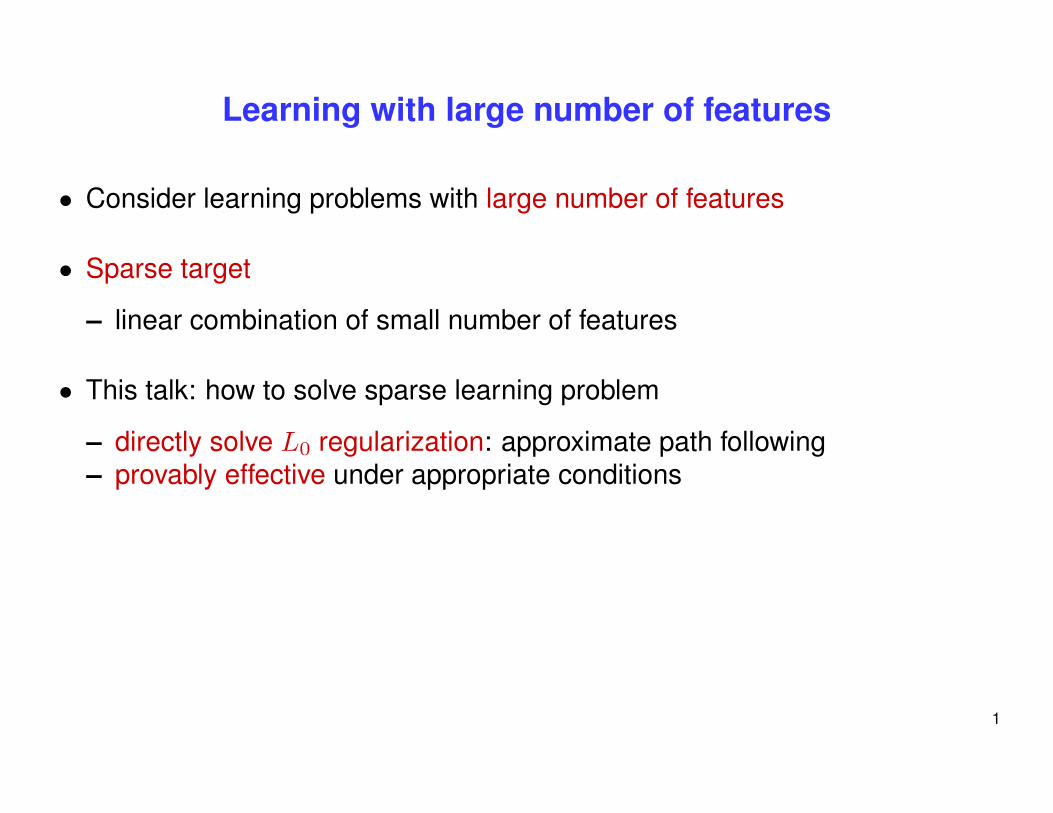
Learning with large number of features

• Consider learning problems with large number of features

• Sparse target

– linear combination of small number of features

• This talk: how to solve sparse learning problem

– directly solve L0 regularization: approximate path following– provably effective under appropriate conditions

1

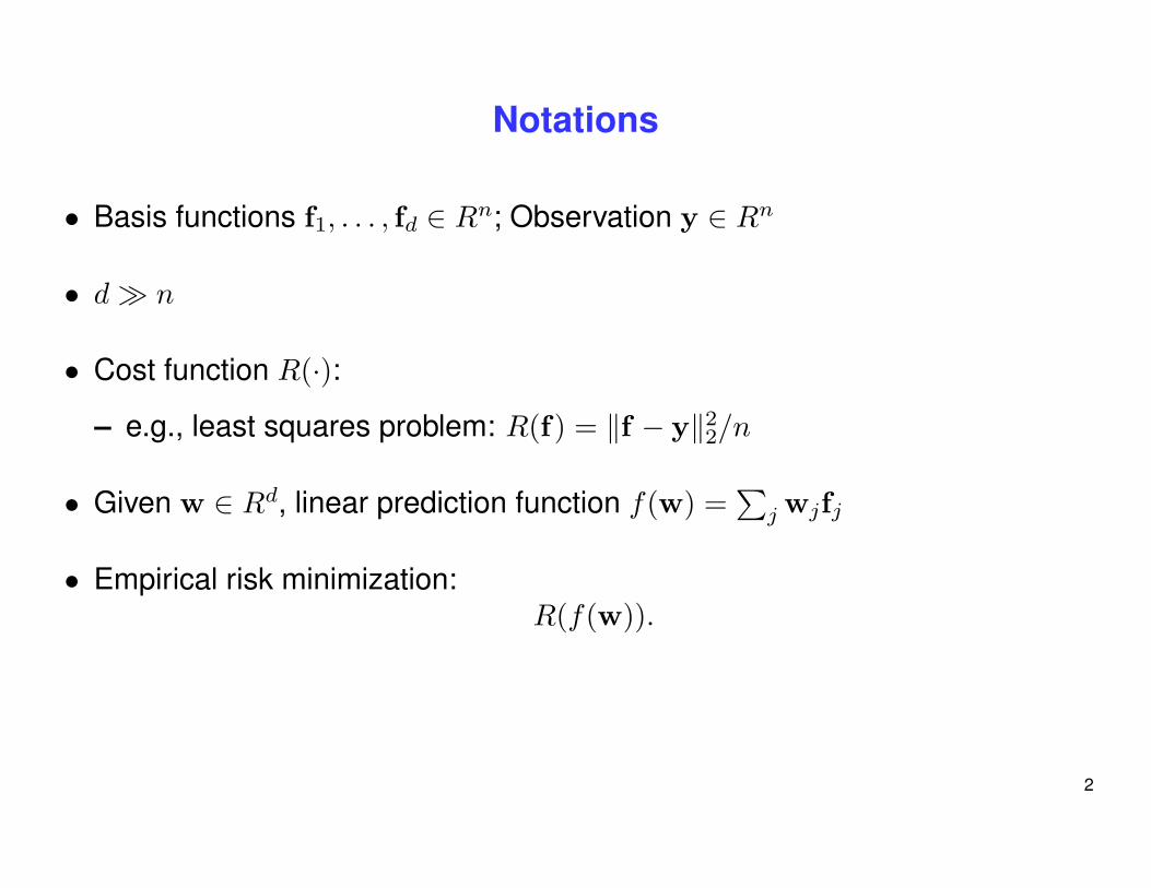
Notations

• Basis functions f1, . . . , fd ∈ Rn; Observation y ∈ Rn

• d � n

• Cost function R(·):

– e.g., least squares problem: R(f) = ‖f − y‖22/n

• Given w ∈ Rd, linear prediction function f(w) =∑

j wjfj

• Empirical risk minimization:R(f(w)).

2

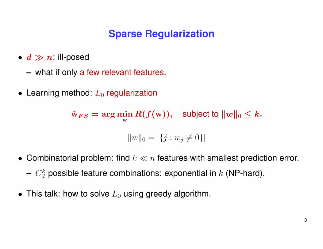
Sparse Regularization

• d � n: ill-posed

– what if only a few relevant features.

• Learning method: L0 regularization

wF S = arg minw

R(f(w)), subject to ‖w‖0 ≤ k.

‖w‖0 = |{j : wj 6= 0}|

• Combinatorial problem: find k � n features with smallest prediction error.

– Ckd possible feature combinations: exponential in k (NP-hard).

• This talk: how to solve L0 using greedy algorithm.

3

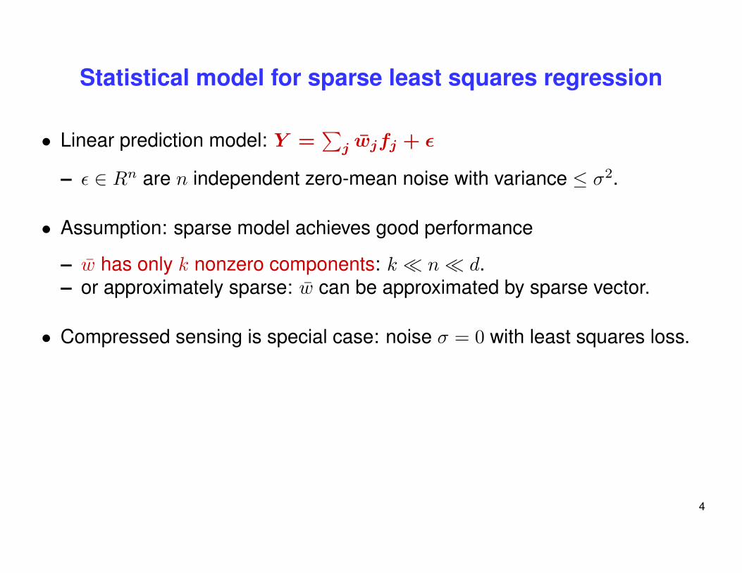
Statistical model for sparse least squares regression

• Linear prediction model: Y =∑

j wjfj + ε

– ε ∈ Rn are n independent zero-mean noise with variance ≤ σ2.

• Assumption: sparse model achieves good performance

– w has only k nonzero components: k � n � d.– or approximately sparse: w can be approximated by sparse vector.

• Compressed sensing is special case: noise σ = 0 with least squares loss.

4

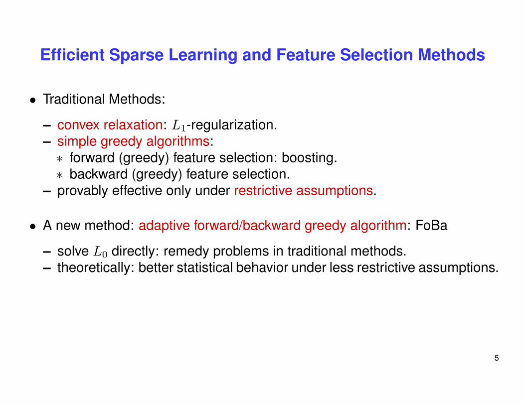
Efficient Sparse Learning and Feature Selection Methods

• Traditional Methods:

– convex relaxation: L1-regularization.– simple greedy algorithms:∗ forward (greedy) feature selection: boosting.∗ backward (greedy) feature selection.

– provably effective only under restrictive assumptions.

• A new method: adaptive forward/backward greedy algorithm: FoBa

– solve L0 directly: remedy problems in traditional methods.– theoretically: better statistical behavior under less restrictive assumptions.

5

Some Assumptions

• sub-Gaussian noise: σ is noise level

• basis are normalized: ‖fj‖2 = 1 (j = 1, . . . , d)

• sparse-eigenvalue conditions: any small number of basis functions arelinearly independent for small k (f(w) =

∑j wjfj)

ρ(k) = inf{

1n‖f(w)‖22/‖w‖22 : ‖w‖0 ≤ k

}> 0,

and for all F ⊂ {1, . . . , d}, let

λ(F ) = sup{

1n‖f(w)‖22/‖w‖22 : support(w) ⊂ F

}.

6

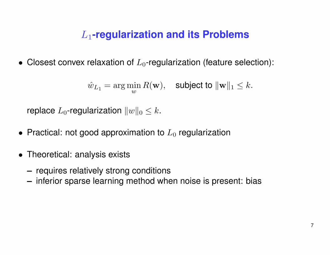
L1-regularization and its Problems

• Closest convex relaxation of L0-regularization (feature selection):

wL1 = arg minw

R(w), subject to ‖w‖1 ≤ k.

replace L0-regularization ‖w‖0 ≤ k.

• Practical: not good approximation to L0 regularization

• Theoretical: analysis exists

– requires relatively strong conditions– inferior sparse learning method when noise is present: bias

7

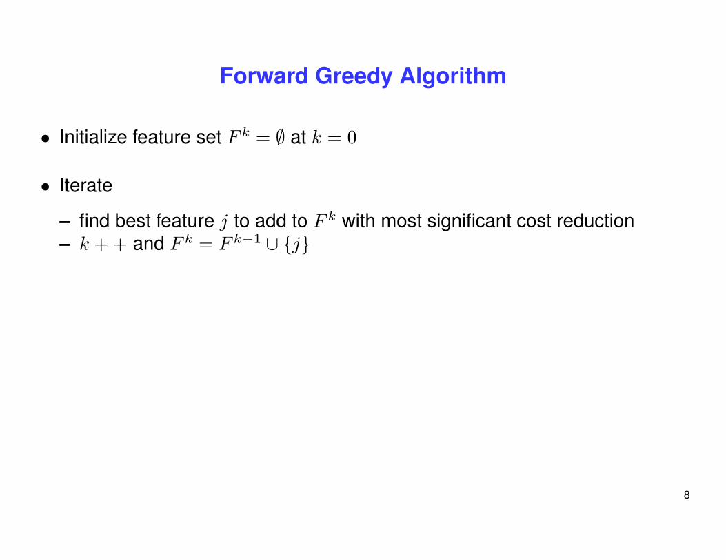
Forward Greedy Algorithm

• Initialize feature set F k = ∅ at k = 0

• Iterate

– find best feature j to add to F k with most significant cost reduction– k + + and F k = F k−1 ∪ {j}

8

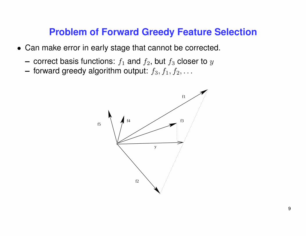
Problem of Forward Greedy Feature Selection

• Can make error in early stage that cannot be corrected.

– correct basis functions: f1 and f2, but f3 closer to y– forward greedy algorithm output: f3, f1, f2, . . .

f5

y

f1

f2

f3f4

9

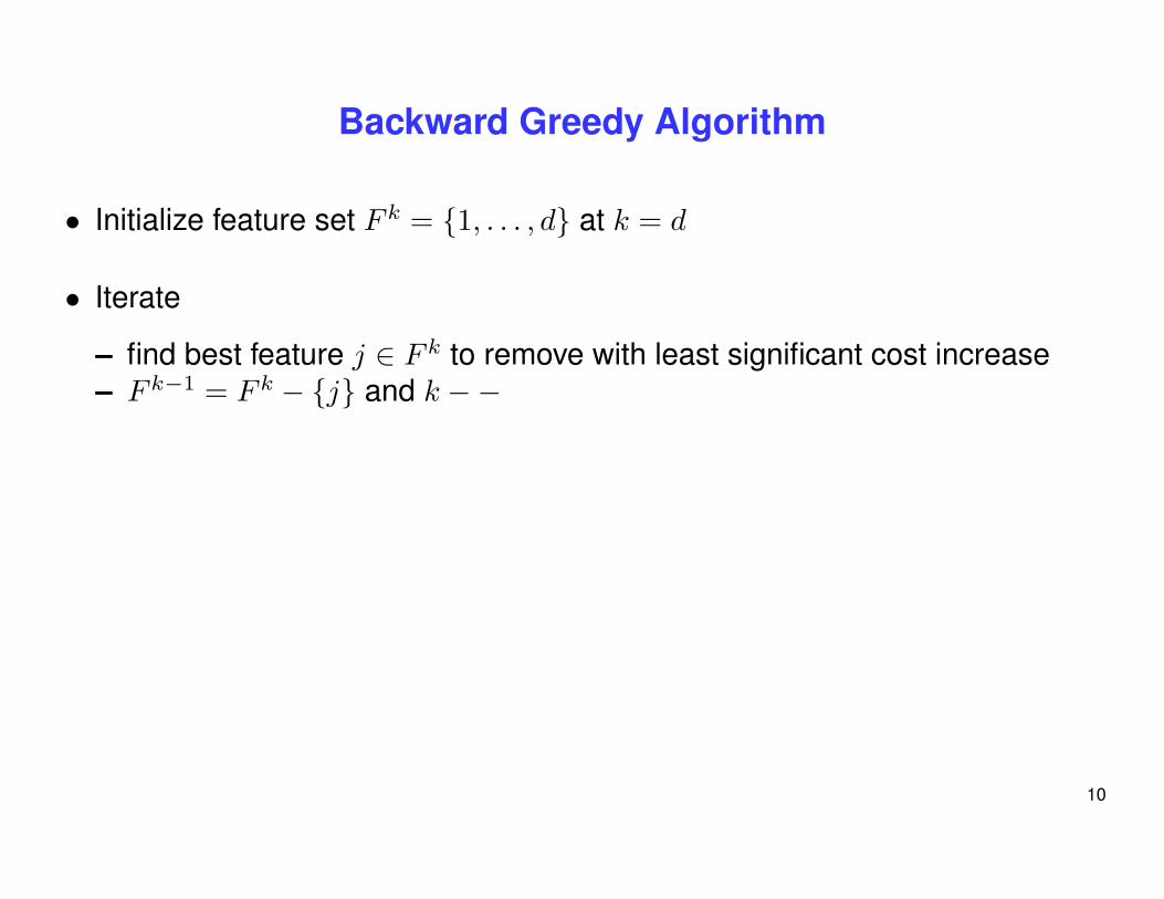
Backward Greedy Algorithm

• Initialize feature set F k = {1, . . . , d} at k = d

• Iterate

– find best feature j ∈ F k to remove with least significant cost increase– F k−1 = F k − {j} and k −−

10

Problems of Backward Greedy Feature Selection

• Computationally very expensive.

• The naive version overfits the data when d � n: R(F d) = 0.

– fails if R(F d − {j}) = 0 for all j ∈ Ft.– cannot effectively eliminate bad features

• Works only when n � d (insignificant overfitting).

– when n � d: have to regularize the naive version to prevent overfitting– how to regularize?

11

Idea: Combine Forward/Backward Algorithms

• Forward greedy

– pros: computationally efficient; doesn’t overfit– cons: error made in early stage doesn’t get corrected later

• Backward greedy

– pros: can correct error by looking at the full model– cons: need to start with sparse/non-overfited model

• Combination: adaptive forward/backward greedy

– computationally efficient; doesn’t overfit; error made in early stage can becorrected by backward greedy step later

– key design issue: when to take a backward step?

12

Greedy method for Direct L0 minimization

• Optimize objective function greedily:

minw

[R(w) + λ‖w‖0].

• Two types of greedy operations to reduce L0 regularized objective

– feature addition (forward): R(w) decreases, λ‖w‖0 increases by λ– feature deletion (backward): R(w) increases, λ‖w‖0 decreases by λ

• First idea: alternating with addition/deletion to reduce objective

– “local” solution: a fixed point of the procedure– problem: ineffective deletion with small λ: overfitting like backward greedy

• Key modification: track a sparse solution path

– L0 path-following: λ decreases from ∞ to 0.

13

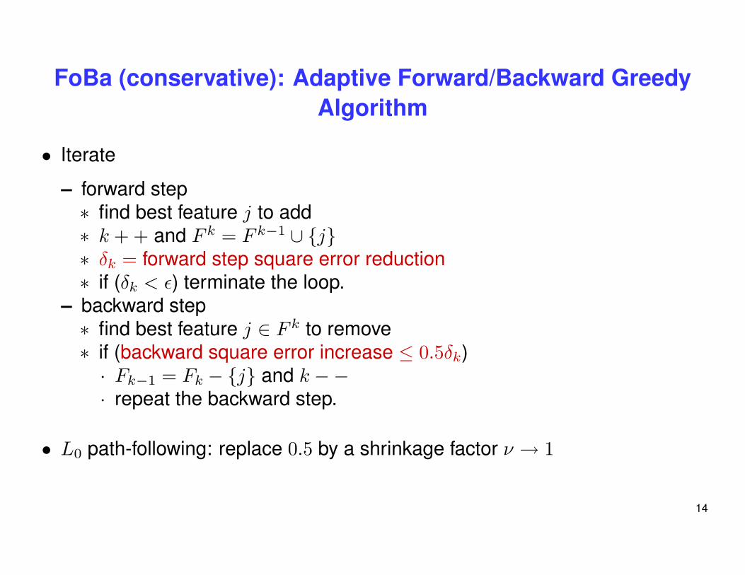
FoBa (conservative): Adaptive Forward/Backward GreedyAlgorithm

• Iterate

– forward step∗ find best feature j to add∗ k + + and F k = F k−1 ∪ {j}∗ δk = forward step square error reduction∗ if (δk < ε) terminate the loop.

– backward step∗ find best feature j ∈ F k to remove∗ if (backward square error increase ≤ 0.5δk)· Fk−1 = Fk − {j} and k −−· repeat the backward step.

• L0 path-following: replace 0.5 by a shrinkage factor ν → 1

14

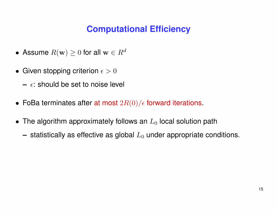
Computational Efficiency

• Assume R(w) ≥ 0 for all w ∈ Rd

• Given stopping criterion ε > 0

– ε: should be set to noise level

• FoBa terminates after at most 2R(0)/ε forward iterations.

• The algorithm approximately follows an L0 local solution path

– statistically as effective as global L0 under appropriate conditions.

15

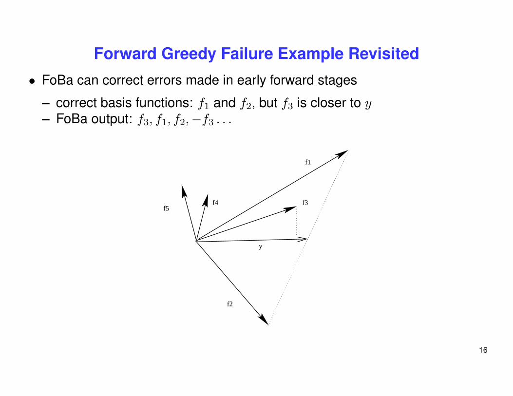
Forward Greedy Failure Example Revisited

• FoBa can correct errors made in early forward stages

– correct basis functions: f1 and f2, but f3 is closer to y– FoBa output: f3, f1, f2,−f3 . . .

f5

y

f1

f2

f3f4

16

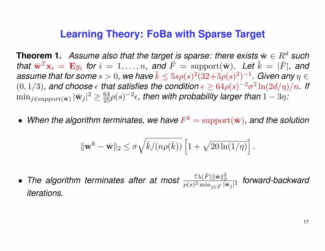
Learning Theory: FoBa with Sparse Target

Theorem 1. Assume also that the target is sparse: there exists w ∈ Rd suchthat wTxi = Eyi for i = 1, . . . , n, and F = support(w). Let k = |F |, andassume that for some s > 0, we have k ≤ 5sρ(s)2(32+5ρ(s)2)−1. Given any η ∈(0, 1/3), and choose ε that satisfies the condition ε ≥ 64ρ(s)−2σ2 ln(2d/η)/n. Ifminj∈support(w) |wj|2 ≥ 64

25ρ(s)−2ε, then with probability larger than 1− 3η:

• When the algorithm terminates, we have F k = support(w), and the solution

‖wk − w‖2 ≤ σ√

k/(nρ(k))[1 +

√20 ln(1/η)

].

• The algorithm terminates after at most 7λ(F )‖w‖22

ρ(s)2 minj∈F |wj|2forward-backward

iterations.

17

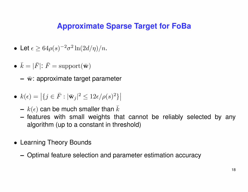
Approximate Sparse Target for FoBa

• Let ε ≥ 64ρ(s)−2σ2 ln(2d/η)/n.

• k = |F |: F = support(w)

– w: approximate target parameter

• k(ε) =∣∣{j ∈ F : |wj|2 ≤ 12ε/ρ(s)2}

∣∣– k(ε) can be much smaller than k– features with small weights that cannot be reliably selected by any

algorithm (up to a constant in threshold)

• Learning Theory Bounds

– Optimal feature selection and parameter estimation accuracy

18

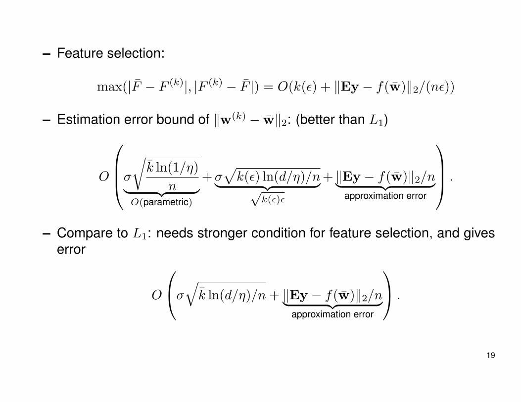
– Feature selection:

max(|F − F (k)|, |F (k) − F |) = O(k(ε) + ‖Ey − f(w)‖2/(nε))

– Estimation error bound of ‖w(k) − w‖2: (better than L1)

O

σ

√k ln(1/η)

n︸ ︷︷ ︸O(parametric)

+σ√

k(ε) ln(d/η)/n︸ ︷︷ ︸√k(ε)ε

+ ‖Ey − f(w)‖2/n︸ ︷︷ ︸approximation error

.

– Compare to L1: needs stronger condition for feature selection, and giveserror

O

σ√

k ln(d/η)/n + ‖Ey − f(w)‖2/n︸ ︷︷ ︸approximation error

.

19

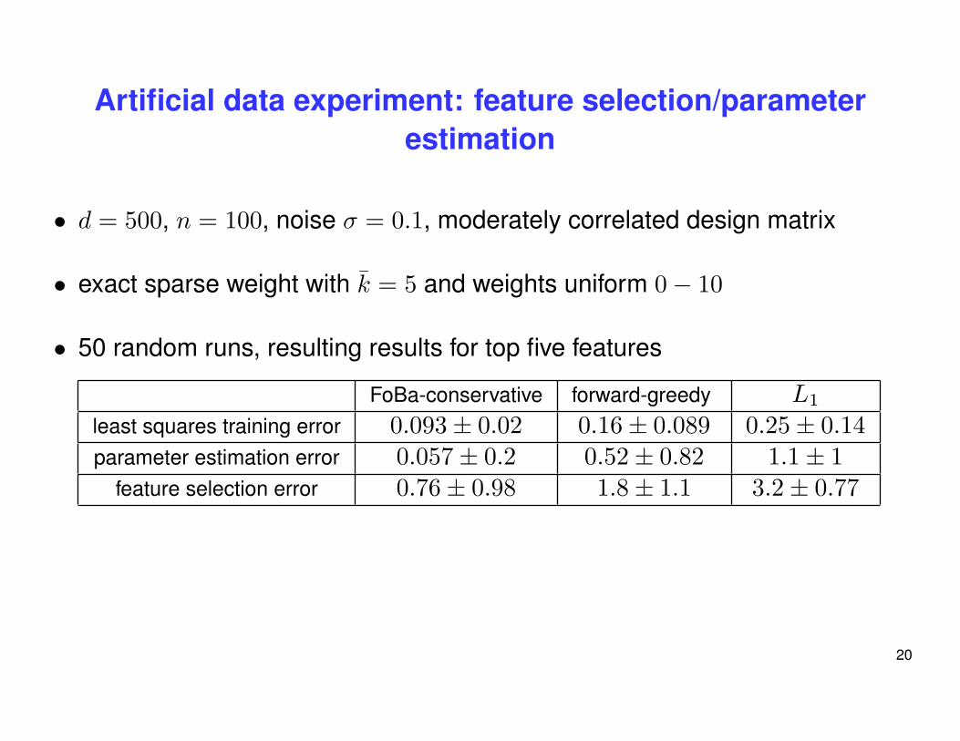
Artificial data experiment: feature selection/parameterestimation

• d = 500, n = 100, noise σ = 0.1, moderately correlated design matrix

• exact sparse weight with k = 5 and weights uniform 0− 10

• 50 random runs, resulting results for top five features

FoBa-conservative forward-greedy L1

least squares training error 0.093± 0.02 0.16± 0.089 0.25± 0.14parameter estimation error 0.057± 0.2 0.52± 0.82 1.1± 1

feature selection error 0.76± 0.98 1.8± 1.1 3.2± 0.77

20

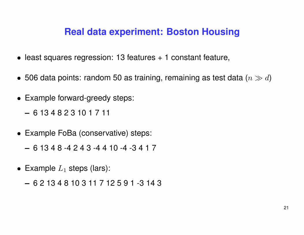
Real data experiment: Boston Housing

• least squares regression: 13 features + 1 constant feature,

• 506 data points: random 50 as training, remaining as test data (n � d)

• Example forward-greedy steps:

– 6 13 4 8 2 3 10 1 7 11

• Example FoBa (conservative) steps:

– 6 13 4 8 -4 2 4 3 -4 4 10 -4 -3 4 1 7

• Example L1 steps (lars):

– 6 2 13 4 8 10 3 11 7 12 5 9 1 -3 14 3

21

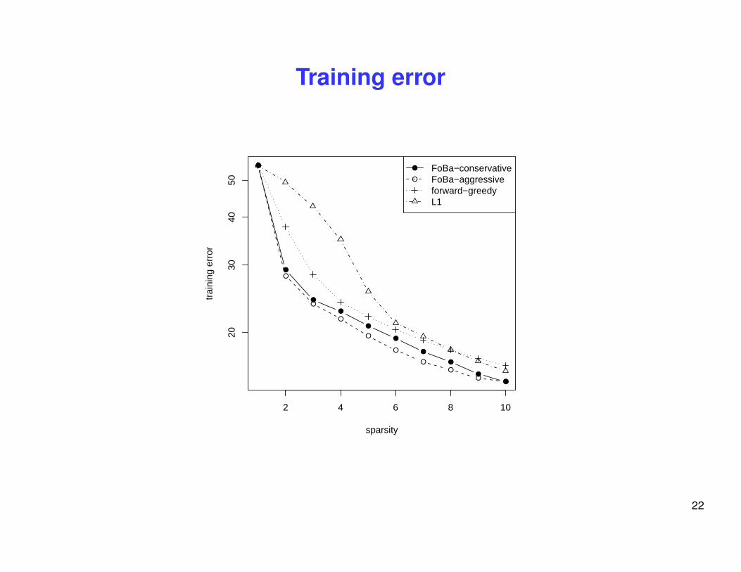
Training error

●

●

●

●

●

●

●

●

●

●

2 4 6 8 10

2030

4050

sparsity

trai

ning

err

or

●

●

●

●

●

●

●

●

●●

●

●

FoBa−conservativeFoBa−aggressiveforward−greedyL1

22

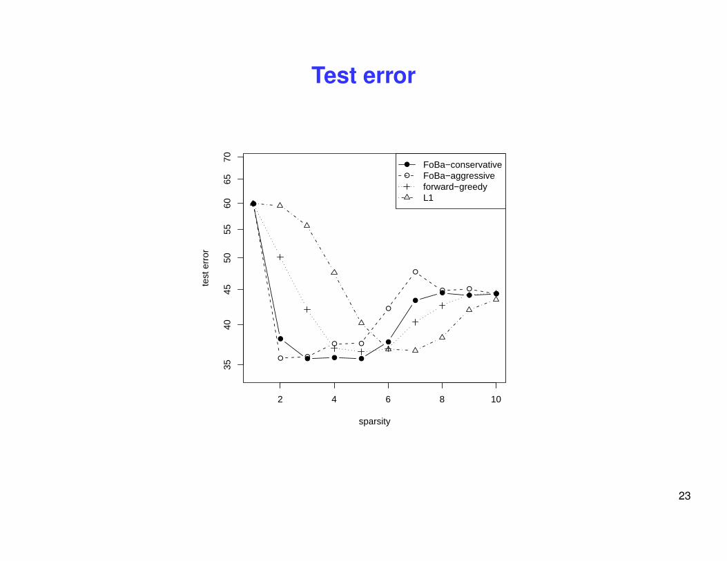
Test error

●

●

● ● ●

●

●

● ● ●

2 4 6 8 10

3540

4550

5560

6570

sparsity

test

err

or●

● ●

● ●

●

●

● ●●

●

●

FoBa−conservativeFoBa−aggressiveforward−greedyL1

23

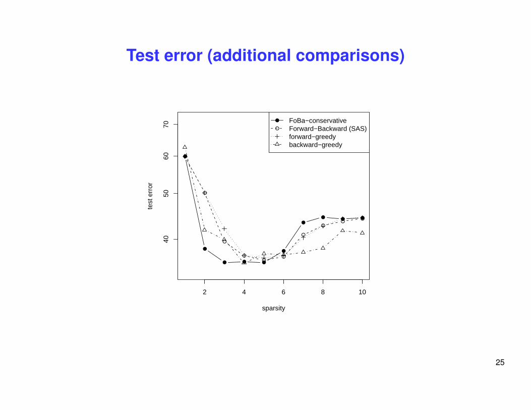
Training error (additional comparisons)

●

●

●

●

●

●

●

●

●

●

2 4 6 8 10

2030

4050

sparsity

trai

ning

err

or

●

●

●

●

●

●

●●

●●

●

●

FoBa−conservativeForward−Backward (SAS)forward−greedybackward−greedy

24

Test error (additional comparisons)

●

●

● ● ●

●

●

● ● ●

2 4 6 8 10

4050

6070

sparsity

test

err

or●

●

●

●●

●

●

●●

●

●

●

FoBa−conservativeForward−Backward (SAS)forward−greedybackward−greedy

25

Summary

• Traditional approximation methods for L0 regularization

– L1 relaxation (bias: need non-convexity)– forward selection (not good for feature selection)– backward selection (cannot start with overfitted model)

• FoBa: combines the strength of forward backward selection

– approximate path-following algorithm to directly solve L0

– theoretically: more effective than earlier algorithms– practically: closer to L0 than forward-greedy and L1

• A Final Remark: L0 (sparsity) does not always lead to better predictionperformance in practice (unstable for certain problems)

26