3/9/2006 16.75 1

Airline Fleet Assignment

Cynthia Barnhart16.75 Airline Management

Outline:– Problem Definition and Objective– Fleet Assignment Network Representation– Fleet Assignment Models and Algorithms– Extension of Fleet Assignment to Schedule Design– Conclusions

3/9/2006 16.75 2

Airline Schedule Planning

Select optimal set of flight legsin a schedule

Schedule Design

Route individual aircraft honoringmaintenance restrictions

Assign aircraft types to flight legs such that contribution is maximizedA flight specifies origin, destination,

and departure timeFleet Assignment

Aircraft Routing Contribution = Revenue - Costs

Crew SchedulingAssign crew (pilots and/or flight

attendants) to flight legs

3/9/2006 16.75 3

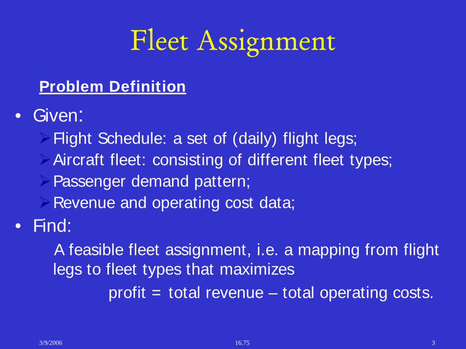
Fleet AssignmentProblem Definition

• Given:Flight Schedule: a set of (daily) flight legs;Aircraft fleet: consisting of different fleet types;Passenger demand pattern;Revenue and operating cost data;

• Find:A feasible fleet assignment, i.e. a mapping from flight legs to fleet types that maximizes

profit = total revenue – total operating costs.

3/9/2006 16.75 4

Fleet Assignment• Class Exercise: Flight Network

LGA

BOS

ORD

Boston Logan

New York LaGuardia

CL30x(3 flights)

CL33x(3 flights)

CL55x(2 flights)

CL50x(2 flights)

Chicago O’Hare

3/9/2006 16.75 5

Fleet Assignment

• Class Exercise: Flight Schedule, Fares, & Demand

Flight # From To Dept Time (EST)

Arr Time (EST)

Fare [$]

Demand [passengers]

CL301 LGA BOS 1000 1100 150 250 CL302 LGA BOS 1100 1200 150 250 CL303 LGA BOS 1800 1900 150 100 CL331 BOS LGA 0700 0800 150 150 CL332 BOS LGA 1030 1130 150 300 CL333 BOS LGA 1800 1900 150 150 CL501 LGA ORD 1100 1400 400 150 CL502 LGA ORD 1500 1800 400 200 CL551 ORD LGA 0700 1000 400 200 CL552 ORD LGA 0830 1130 400 150

3/9/2006 16.75 6

Fleet Assignment

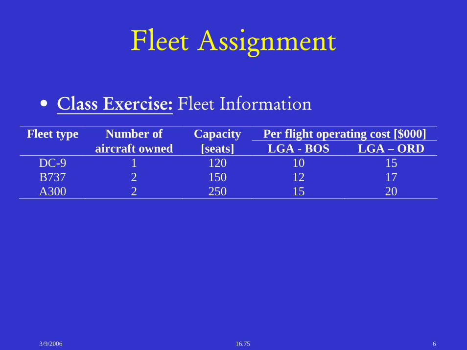
• Class Exercise: Fleet InformationFleet type Number of Capacity Per flight operating cost [$000]

aircraft owned [seats] LGA - BOS LGA – ORD DC-9 1 120 10 15 B737 2 150 12 17 A300 2 250 15 20

3/9/2006 16.75 7

Fleet Assignment

• Class Exercise:

Find:An assignment of fleet types to the

flights in this network that maximizes net profit.

3/9/2006 16.75 8

Fleet Assignment

Evaluating assignment profits:

flfllfl OpCostCapDfarec ,, ),min(: −×=where:where:

. legflight to fleet type assigning ofcost operating :

; fleet type ofcapacity :; legflight of demand :

; legflight of fare :

;legflight to fleet typeassigningofity profitabil :

,

,

lfOpCost

fCaplD

lfare

lfc

fl

f

l

l

fl

3/9/2006 16.75 9

Fleet Assignment• Class Exercise: Evaluating assignment

profitabilities…Profitability [$000 per day]

Flight # DC-9 B737 A300 CL301 8 10.5 22.5 CL302 8 10.5 22.5 CL303 5 3 0 CL331 8 10.5 7.5 CL332 8 10.5 22.5 CL333 8 10.5 7.5 CL501 33 43 40 CL502 33 43 60 CL551 33 43 60 CL552 33 43 40

3/9/2006 16.75 10

Fleet AssignmentTime-Line Network:

BOS

CL331

CL301

CL302 CL303

CL332 CL333

CL551CL552 CL501

CL502

LGA

ORD

0800 1000 1200 1400 1600timescale

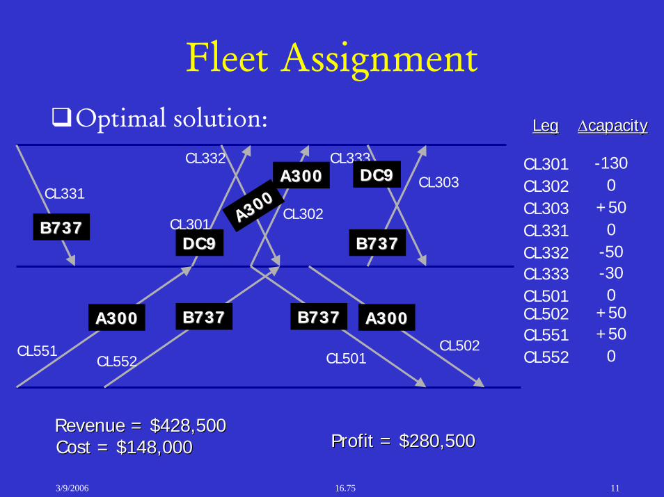
3/9/2006 16.75 11

Fleet AssignmentOptimal solution: LegLeg ∆∆capacitycapacity

CL301CL302CL303CL331CL332CL333CL501CL502CL551CL552

CL331

CL301CL302

CL303

CL332 CL333

CL551CL552 CL501

CL502

A300A300 A300A300B737B737B737B737

DC9DC9 B737B737A300A300

DC9DC9A300A300

B737B737

-1300

+500

-50-300

+50+50

0

Revenue = $428,500 Revenue = $428,500 Cost = $148,000Cost = $148,000 Profit = $280,500Profit = $280,500

3/9/2006 16.75 12

Fleet AssignmentTime-Line Network:

Airport AAirport A

Airport BAirport B

Flight arc

v−vy +vy

wl,f

Ground arc

count line

3/9/2006 16.75 13

Notations• Decision Variables

– fk,i equals 1 if fleet type k is assigned to flight leg i, and 0 otherwise

– yk,o,t is the number of aircraft of fleet type k, on the ground at station o, and time t

• Parameters– Ck,i is the cost of assigning fleet k to flight leg i– Nk is the number of available aircraft of fleet type k – tn is the “count time”

• Sets– L is the set of all flight legs i– K is the set of all fleet types k– O is the set of all stations o– CL(k) is the set of all flight arcs for fleet type k crossing the

count time

3/9/2006 16.75 14

Fleet Assignment Model (FAM)

Kk∈∀

∑ ∑∈ ∈Kk Li

ikik fcMin ,,

1, =∑∈Kk

ikf

0),,(

,,,),,(

,,, =−−+ ∑∑∈∈

+−

tokOiiktok

tokIiiktok fyfy

kkCLi

ikOo

tok Nfyn

≤+ ∑∑∈∈ )(

,,,

{ }1,0, ∈ikf 0,, ≥toky

Li∈∀

tok ,,∀

Subject to:

Kk∈∀

∑ ∑∈ ∈Kk Li

ikik fcMin ,,

1, =∑∈Kk

ikf

0),,(

,,,),,(

,,, =−−+ ∑∑∈∈

+−

tokOiiktok

tokIiiktok fyfy

kkCLi

ikOo

tok Nfyn

≤+ ∑∑∈∈ )(

,,,

{ }1,0, ∈ikf 0,, ≥toky

Li∈∀

tok ,,∀

Subject to:

Kk∈∀

∑ ∑∈ ∈Kk Li

ikik fcMin ,,

1, =∑∈Kk

ikf

0),,(

,,,),,(

,,, =−−+ ∑∑∈∈

+−

tokOiiktok

tokIiiktok fyfy

kkCLi

ikOo

tok Nfyn

≤+ ∑∑∈∈ )(

,,,

{ }1,0, ∈ikf 0,, ≥toky

Li∈∀

tok ,,∀

Subject to:

Hane et al. (1995), Abara (1989), and Jacobs, Smith and Johnson (2000)

3/9/2006 16.75 15

Constraints• Cover Constraints

– Each flight must be assigned to exactly one fleet

• Balance Constraints– Number of aircraft of a fleet type arriving at

a station must equal the number of aircraft of that fleet type departing

• Aircraft Count Constraints– Number of aircraft of a fleet type used

cannot exceed the number available

3/9/2006 16.75 16

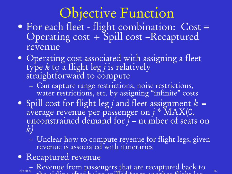
Objective Function• For each fleet - flight combination: Cost ≡

Operating cost + Spill cost –Recaptured revenue

• Operating cost associated with assigning a fleet type k to a flight leg j is relatively straightforward to compute– Can capture range restrictions, noise restrictions,

water restrictions, etc. by assigning “infinite” costs• Spill cost for flight leg j and fleet assignment k =

average revenue per passenger on j * MAX(0, unconstrained demand for j – number of seats on k)– Unclear how to compute revenue for flight legs, given

revenue is associated with itineraries• Recaptured revenue

– Revenue from passengers that are recaptured back to the airline after being spilled from another flight leg

3/9/2006 16.75 17

FAM Example: Spill

A B

Demand = 100Fare = $100

Revenue

$8,000

$10,000

$10,000

$10,000

Capacity

80

100

120

150

Fleet Type

i

ii

iii

iv

Contribution

$3,000

$4,000

$3,000

$2,000

Assignment Cost

$7,000

$6,000

$7,000

$8,000

Op. Cost

$5,000

$6,000

$7,000

$8,000

Spill Cost

$2,000

$0

$0

$0

3/9/2006 16.75 18

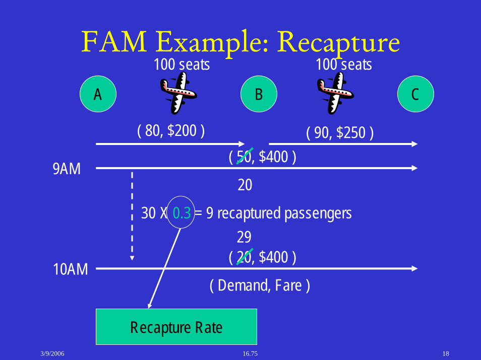
( 50, $400 )9AM

FAM Example: Recapture

A B C

( 80, $200 ) ( 90, $250 )

( Demand, Fare )

30

20

( 20, $400 )10AM

Recapture Rate

X 0.3 = 9 recaptured passengers29

100 seats 100 seats

3/9/2006 16.75 19

Fleet Assignment

A few observations on FAM:Nodes can be consolidated to reduce model size;Fleet-specific time-line networks are possible;Fleet assignment not aircraft assignment! Note that feasibility of FAM implies that aircraft rotations exist (takes only a little bit of thinking);However, these rotations might not be maintenance feasible…

3/9/2006 16.75 20

Fleet Assignment

Solvability:FAM can be solved using standard branch-and-bound software;Solution times are FAST, thanks to FAM’s small LP gaps…

3/9/2006 16.75 21

Fleet Assignment

Computational Sample: 2,044 flight legs, 9 fleet types2,044 flight legs, 9 fleet types

Problem size# of columns 18,487# of rows 7,827# of non-zero entries 50,034

Strength of formulationRoot node LP solution 21,401,658Best IP solution 21,401,622Difference 36

Solution time [sec] 974

3/9/2006 16.75 22

Fleet Assignment

• FAM suffers from a significant drawback in its modeling of the revenue side…

• Passengers book itineraries not flight legs…

• Capacity decisions on one leg will affect passenger spill on other legs…

• This phenomenon is known as network effects.

3/9/2006 16.75 23

Fleet Assignment Model (FAM)

Kk∈∀

∑ ∑∈ ∈Kk Li

ikik fcMin ,,

1, =∑∈Kk

ikf

0),,(

,,,),,(

,,, =−−+ ∑∑∈∈

+−

tokOiiktok

tokIiiktok fyfy

kkCLi

ikOo

tok Nfyn

≤+ ∑∑∈∈ )(

,,,

{ }1,0, ∈ikf 0,, ≥toky

Li∈∀

tok ,,∀

Subject to:

Kk∈∀

∑ ∑∈ ∈Kk Li

ikik fcMin ,,

1, =∑∈Kk

ikf

0),,(

,,,),,(

,,, =−−+ ∑∑∈∈

+−

tokOiiktok

tokIiiktok fyfy

kkCLi

ikOo

tok Nfyn

≤+ ∑∑∈∈ )(

,,,

{ }1,0, ∈ikf 0,, ≥toky

Li∈∀

tok ,,∀

Subject to:

Kk∈∀

∑ ∑∈ ∈Kk Li

ikik fcMin ,,

1, =∑∈Kk

ikf

0),,(

,,,),,(

,,, =−−+ ∑∑∈∈

+−

tokOiiktok

tokIiiktok fyfy

kkCLi

ikOo

tok Nfyn

≤+ ∑∑∈∈ )(

,,,

{ }1,0, ∈ikf 0,, ≥toky

Li∈∀

tok ,,∀

Subject to:

Major Shortcoming:Major Shortcoming:FAM assumes leg independenceFAM assumes leg independence

Hane et al. (1995), Abara (1989), and Jacobs, Smith and Johnson (2000)

3/9/2006 16.75 24

FAM Example: Network Effects

A B C

( 50, $400 )( 80, $200 ) ( 90, $250 )

( Demand, Fare )

Spill Cost

?

?

?

$0

Fleet Type

i

ii

iii

iv

Capacity

80

100

120

150

Leg Interdependence

Network Effects

3/9/2006 16.75 25

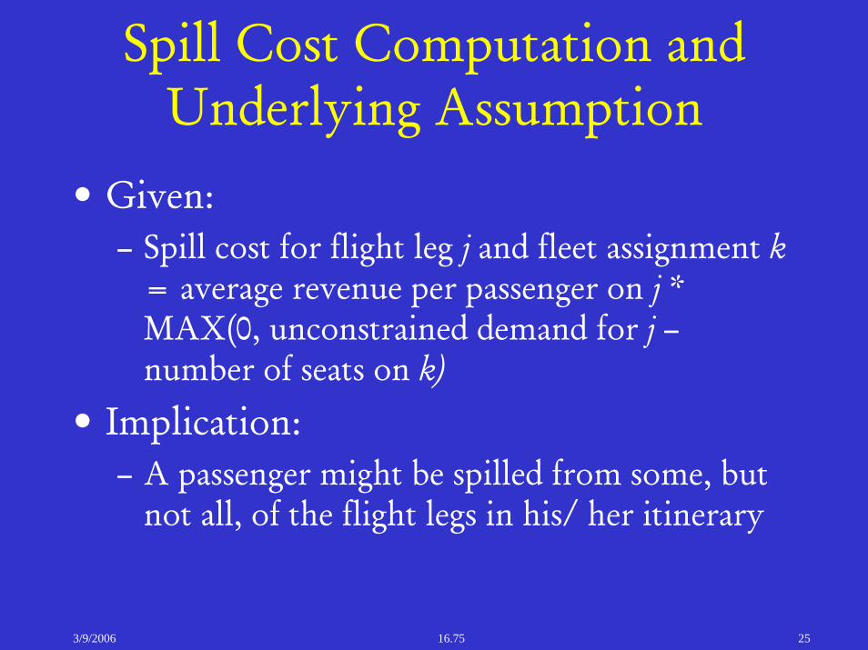
Spill Cost Computation and Underlying Assumption

• Given: – Spill cost for flight leg j and fleet assignment k

= average revenue per passenger on j * MAX(0, unconstrained demand for j –number of seats on k)

• Implication: – A passenger might be spilled from some, but

not all, of the flight legs in his/ her itinerary

3/9/2006 16.75 26

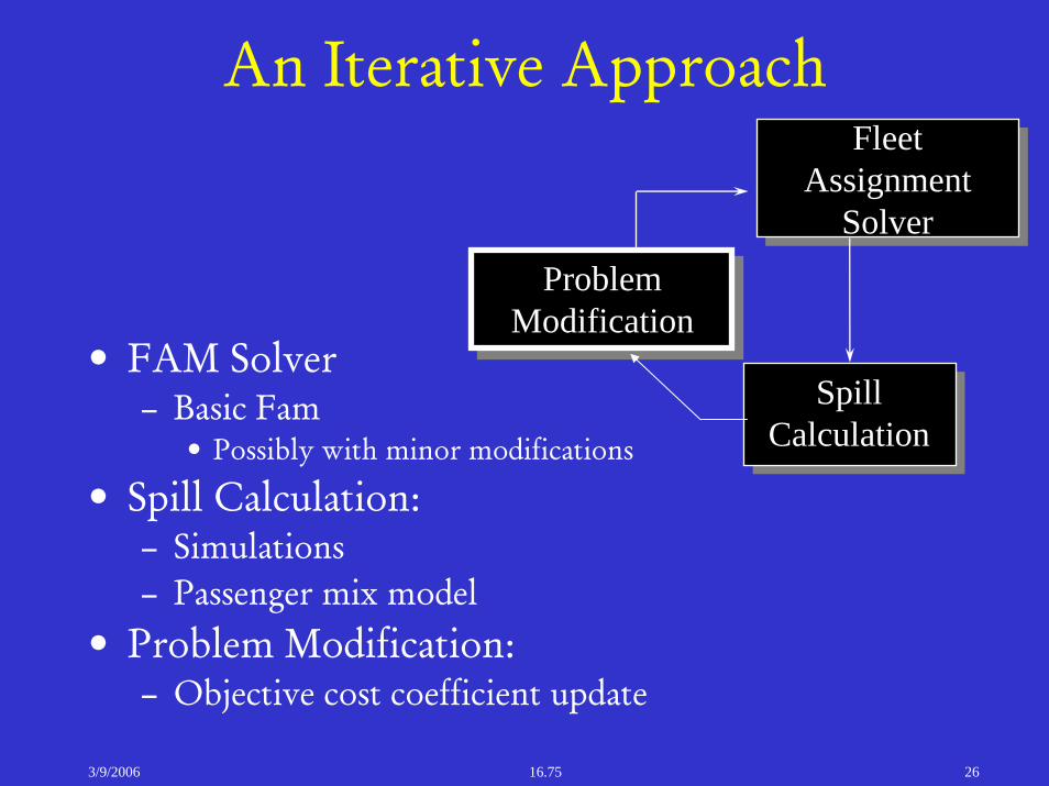
An Iterative ApproachFleet

AssignmentSolver

SpillCalculation

ProblemModification

• FAM Solver– Basic Fam

• Possibly with minor modifications

• Spill Calculation: – Simulations – Passenger mix model

• Problem Modification: – Objective cost coefficient update

3/9/2006 16.75 27

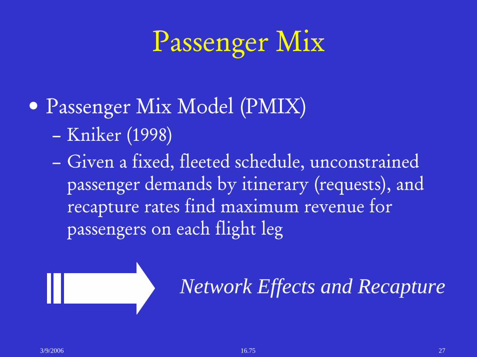
Passenger Mix

• Passenger Mix Model (PMIX)– Kniker (1998)– Given a fixed, fleeted schedule, unconstrained

passenger demands by itinerary (requests), and recapture rates find maximum revenue for passengers on each flight leg

Network Effects and RecapturePMIX

3/9/2006 16.75 28

Problem Modification

• Based on differences in expected spill from FAM and the Spill Calculator, we modify the FAM problem– Update objective cost coefficients

• Cost coefficient update, many heuristics possible

3/9/2006 16.75 29

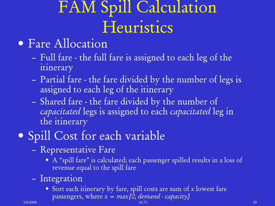
FAM Spill Calculation Heuristics

• Fare Allocation– Full fare - the full fare is assigned to each leg of the

itinerary– Partial fare - the fare divided by the number of legs is

assigned to each leg of the itinerary– Shared fare - the fare divided by the number of

capacitated legs is assigned to each capacitated leg in the itinerary

• Spill Cost for each variable– Representative Fare

• A “spill fare” is calculated; each passenger spilled results in a loss of revenue equal to the spill fare

– Integration• Sort each itinerary by fare, spill costs are sum of x lowest fare

passengers, where x = max{0, demand - capacity}

3/9/2006 16.75 30

An Illustrative ExampleX Y Z

flight 1 flight 2Fleet Type Seats

A 100B 200

MarketAverage

FareItineraryNo. of

Pax1 $200X-Y 75

$225Y-Z 2 150X-Z 1-2 $300 75

$30,000 $38,125A-A 50 X-Z, 75 Y-Z

$15,625A-B $11,250

B-A $22,500 $28,125

Fleet Assign. Full Alloc.Partial Alloc. Actual Opt.

B-B $3,750 $5,625

Fl. 1- Fl. 2 SpillSpill Spill Spilled Pax31,875

12,500

28,125

5,625

25 X-Z, 25 X-Y

125 Y-Z

25 Y-Z

3/9/2006 16.75 31

Spill Calculation: Results

• For a 3 fleet, 226 flights problem:– The best representative fare solution results in

a gap with the optimal solution of $2,600/day– Using a shared fare scheme and integration

approach, we found a solution with an $8/day gap.

• By simply modifying the basic spill model, significant gains can be achieved

3/9/2006 16.75 32

Itinerary-Based Fleet Assignment

• Impossible to estimate airline profit exactly using link-based costs

• Enhance basic fleet assignment model to include passenger flow decision variables– Associate operating costs with fleet

assignment variables– Associate revenues with passenger flow

variables

3/9/2006 16.75 33

Itinerary-based Fleet Assignment Definition

• Given– a fixed schedule, – number of available aircraft of different types, – unconstrained passenger demands by

itinerary, and– recapture rates,

Find maximum contribution

Network effectsODFAM

3/9/2006 16.75 34

Kk ∈∀

, , ( )r rk i k i p p r p

k K i L p P r PM in c f fare b fare t

∈ ∈ ∈ ∈

+ −∑ ∑ ∑ ∑%

1, =∑∈Kk

ikf

0),,(

,,,),,(

,,, =−−+ ∑∑∈∈

+−

tokOiiktok

tokIiiktok fyfy

kkCLi

ikOo

tok Nfyn

≤+ ∑∑∈∈ )(

,,,

{ }1,0, ∈ikf 0,, ≥toky

Li ∈∀

tok ,,∀

S u b je c t to :

iPr Pp

rp

rp

pi

Pr Pp

rp

pi

kkik QtbtSEATSf ≥−+ ∑ ∑∑ ∑∑

∈ ∈∈ ∈δδ,

pPr

rp Dt ≤∑

∈

0≥rpt

Li∈∀

Pp ∈∀

Kk ∈∀

, , ( )r rk i k i p p r p

k K i L p P r PM in c f fare b fare t

∈ ∈ ∈ ∈

+ −∑ ∑ ∑ ∑%

1, =∑∈Kk

ikf

0),,(

,,,),,(

,,, =−−+ ∑∑∈∈

+−

tokOiiktok

tokIiiktok fyfy

kkCLi

ikOo

tok Nfyn

≤+ ∑∑∈∈ )(

,,,

{ }1,0, ∈ikf 0,, ≥toky

Li ∈∀

tok ,,∀

S u b je c t to :

iPr Pp

rp

rp

pi

Pr Pp

rp

pi

kkik QtbtSEATSf ≥−+ ∑ ∑∑ ∑∑

∈ ∈∈ ∈δδ,

pPr

rp Dt ≤∑

∈

0≥rpt

Li∈∀

Pp ∈∀

Itinerary-Based FAM (IFAM)

FAMFAM

PMMPMMConsistent Spill + RecaptureConsistent Spill + Recapture

Fleet AssignmentFleet Assignment

Kniker (1998)

3/9/2006 16.75 35

Kk ∈∀

, , ( )r rk i k i p p r p

k K i L p P r PM in c f fare b fare t

∈ ∈ ∈ ∈

+ −∑ ∑ ∑ ∑%

1, =∑∈Kk

ikf

0),,(

,,,),,(

,,, =−−+ ∑∑∈∈

+−

tokOiiktok

tokIiiktok fyfy

kkCLi

ikOo

tok Nfyn

≤+ ∑∑∈∈ )(

,,,

{ }1,0, ∈ikf 0,, ≥toky

Li ∈∀

tok ,,∀

S u b je c t to :

iPr Pp

rp

rp

pi

Pr Pp

rp

pi

kkik QtbtSEATSf ≥−+ ∑ ∑∑ ∑∑

∈ ∈∈ ∈δδ,

pPr

rp Dt ≤∑

∈

0≥rpt

Li∈∀

Pp ∈∀

Kk ∈∀

, , ( )r rk i k i p p r p

k K i L p P r PM in c f fare b fare t

∈ ∈ ∈ ∈

+ −∑ ∑ ∑ ∑%

1, =∑∈Kk

ikf

0),,(

,,,),,(

,,, =−−+ ∑∑∈∈

+−

tokOiiktok

tokIiiktok fyfy

kkCLi

ikOo

tok Nfyn

≤+ ∑∑∈∈ )(

,,,

{ }1,0, ∈ikf 0,, ≥toky

Li ∈∀

tok ,,∀

S u b je c t to :

iPr Pp

rp

rp

pi

Pr Pp

rp

pi

kkik QtbtSEATSf ≥−+ ∑ ∑∑ ∑∑

∈ ∈∈ ∈δδ,

pPr

rp Dt ≤∑

∈

0≥rpt

Li∈∀

Pp ∈∀

Itinerary-Based FAM (IFAM)

1

3

2

Kniker (1998)

3/9/2006 16.75 36

Column and Constraint Generation

Original RMP 1

2

3

4

5

6

7

8

3/9/2006 16.75 37

Implementation Details• Computer

– Workstation class computer

– 2 GB RAM– CPLEX 6.5

• Full size schedule– ~2,000 legs– ~76,000 itineraries– ~21,000 markets– 9 fleet types

• RMP constraint matrix size– ~77,000 columns– ~11,000 rows

• Final size– ~86,000 columns– ~19,800 rows

• Solution time– LP: > 1.5 hours– IP: > 4 hours

88% Saving from Row Generation> 95% Saving from Column Generation

3/9/2006 16.75 38

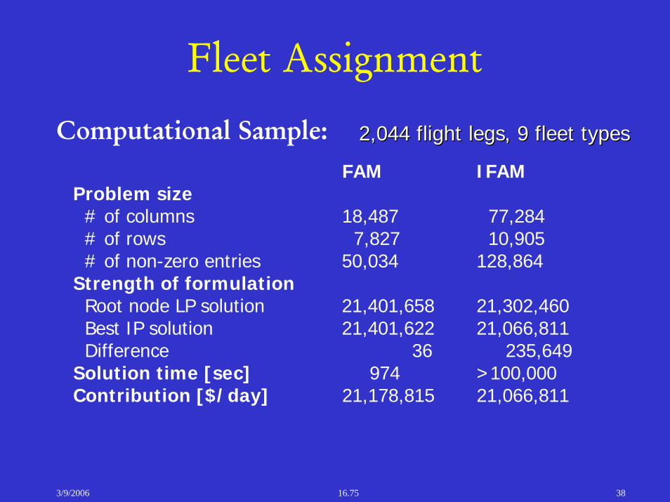
Fleet Assignment

Computational Sample: 2,044 flight legs, 9 fleet types2,044 flight legs, 9 fleet types

FAM IFAMProblem size# of columns 18,487 77,284# of rows 7,827 10,905# of non-zero entries 50,034 128,864

Strength of formulationRoot node LP solution 21,401,658 21,302,460Best IP solution 21,401,622 21,066,811Difference 36 235,649

Solution time [sec] 974 >100,000Contribution [$/day] 21,178,815 21,066,811

3/9/2006 16.75 39

IFAM Contributions

• Annual improvements over basic FAM– Network Effects: ~$30 million– Recapture: ~$70 million

• These estimates are upper bounds on achievable improvements

3/9/2006 16.75 40

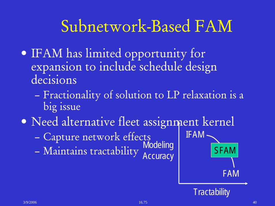
Subnetwork-Based FAM• IFAM has limited opportunity for

expansion to include schedule design decisions– Fractionality of solution to LP relaxation is a

big issue• Need alternative fleet assignment kernel

– Capture network effects– Maintains tractability

Tractability

ModelingAccuracy

FAM

IFAM?SFAM

3/9/2006 16.75 41

FAMIFAM

1

2

3

4

5

6

7

8

9

1

2

3

4

5

6

7

8

9

SFAM

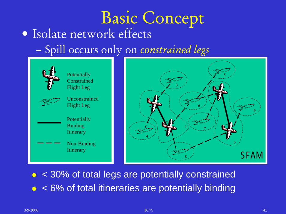
Basic Concept• Isolate network effects

– Spill occurs only on constrained legs

Potentially Constrained Flight Leg

Unconstrained Flight Leg

Potentially Binding Itinerary

Non-Binding Itinerary

Potentially Constrained Flight Leg

Unconstrained Flight Leg

Potentially Binding Itinerary

Non-Binding Itinerary

< 30% of total legs are potentially constrained< 6% of total itineraries are potentially binding

3/9/2006 16.75 42

Modeling Challenges• Utilize composite variables (Armacost, 2000;

Barnhart, Farahat and Lohatepanont, 2001)

11

1 2 3 4 5 6 7 8 9

A A A B B B C C C

A B C A B C A B C

1 2 3 4 5 6 7 8 9

A A A B B B C C C

A B C A B C A B C

3 Fleet Types: A, B, and C

ChallengesEfficient column enumeration

3/9/2006 16.75 43

SFAM Formulation

Kk∈∀

( ) ( )1 1

mS S

S S

Mm m

n nm n

Min C fηΠ

Π Π= =∑∑

( ) ( )1 1

1mS S

S S

M im m

n nm n

fη

δΠ

Π Π= =

=∑∑

( ) ( ) ( ) ( ), ,

, , , ,( , , ) 1 1 ( , , ) 1 1

0m mS SS S

S S S S

M Mk i k im m m mk o t k o tn n n n

i I k o t m n i O k o t m n

y f y fη η

κ κΠ Π

− +Π Π Π Π∈ = = ∈ = =

+ − − =∑ ∑∑ ∑ ∑∑

( ) ( ), ,( ) 1 1

mS S

S Sn

M km mk o t kn n

o A i CL k m ny f N

η

γΠ

Π Π∈ ∈ = =

+ ≤∑ ∑ ∑∑

( ) { }0,1Sm

nfΠ

∈ 0,, ≥toky

Li∈∀

tok ,,∀

Subject to:

Kk∈∀

( ) ( )1 1

mS S

S S

Mm m

n nm n

Min C fηΠ

Π Π= =∑∑

( ) ( )1 1

1mS S

S S

M im m

n nm n

fη

δΠ

Π Π= =

=∑∑

( ) ( ) ( ) ( ), ,

, , , ,( , , ) 1 1 ( , , ) 1 1

0m mS SS S

S S S S

M Mk i k im m m mk o t k o tn n n n

i I k o t m n i O k o t m n

y f y fη η

κ κΠ Π

− +Π Π Π Π∈ = = ∈ = =

+ − − =∑ ∑∑ ∑ ∑∑

( ) ( ), ,( ) 1 1

mS S

S Sn

M km mk o t kn n

o A i CL k m ny f N

η

γΠ

Π Π∈ ∈ = =

+ ≤∑ ∑ ∑∑

( ) { }0,1Sm

nfΠ

∈ 0,, ≥toky

Li∈∀

tok ,,∀

Subject to:

FAM solution algorithm applies

3/9/2006 16.75 44

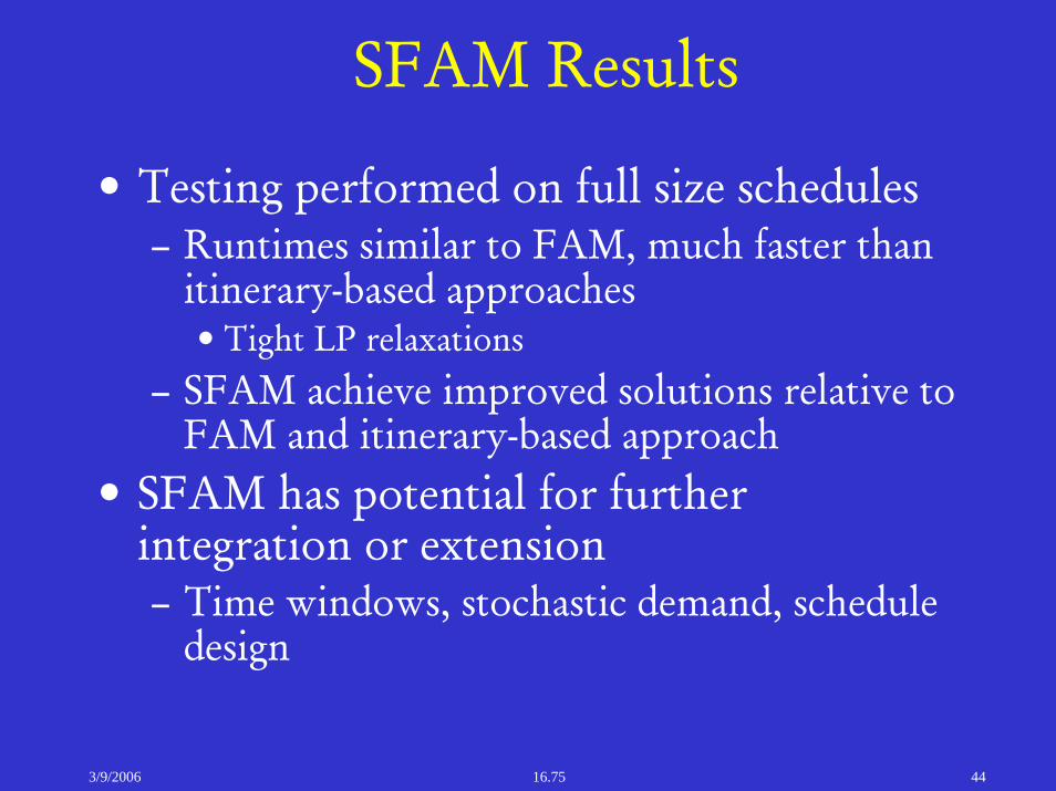
SFAM Results

• Testing performed on full size schedules– Runtimes similar to FAM, much faster than

itinerary-based approaches• Tight LP relaxations

– SFAM achieve improved solutions relative to FAM and itinerary-based approach

• SFAM has potential for further integration or extension– Time windows, stochastic demand, schedule

design

3/9/2006 16.75 45

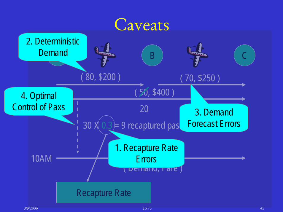
( 50, $400 )9AM

Caveats

A B C

( 80, $200 ) ( 70, $250 )

( Demand, Fare )

X 0.3 = 9 recaptured passengers30

20

( 20, $400 )10AM

Recapture Rate

2. Deterministic Demand

4. Optimal Control of Paxs

1. Recapture Rate Errors

3. Demand Forecast Errors

3/9/2006 16.75 46

Recapture Rate Sensitivity

Fleeting Contribution

EstimatedRevenue

IFAM

Fleeting Decision

Solve PMixwith varied

recapture rates

Solve PMixwith varied

recapture ratesOperating Cost

Specified Recapture Rate

PMix flows passengers on fleeted schedule assuming full knowledge of passenger choices

3/9/2006 16.75 47

Recapture Rate Sensitivity

Recapture Rate Sensitivity

01,0002,0003,0004,0005,0006,0007,0008,000

0.5 0.6 0.7 0.8 0.9 1 1.1 1.2 1.3 1.4 1.5

Recapture Rate Multiplier ( δ)

Impr

ovem

ent o

ver

Bas

ic F

AM

($/d

ay)

Sensitivity of IFAMImprovement gained from network effects aloneImprovement gained from network effects and recapture

3/9/2006 16.75 48

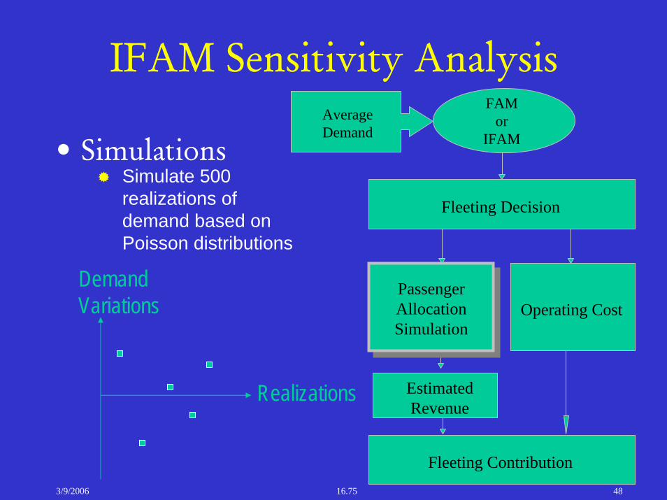
IFAM Sensitivity Analysis

Fleeting Contribution

EstimatedRevenue

• Simulations

FAMor

IFAM

Fleeting Decision

PassengerAllocationSimulation

PassengerAllocationSimulation

Operating Cost

Average Demand

Simulate 500 realizations of demand based on Poisson distributions

Realizations

DemandVariations

3/9/2006 16.75 49

FAM IFAM Difference (IFAM-FAM)Problem 1N-3ARevenue 4,858,089$ 4,918,691$ 60,602$ Operating Cost 2,020,959$ 2,021,300$ 341$ Contribution 2,837,130$ 2,897,391$ 60,261$ Problem 2N-3ARevenue 3,526,622$ 3,513,996$ (12,626)$ Operating Cost 2,255,254$ 2,234,172$ (21,082)$ Contribution 1,271,368$ 1,279,823$ 8,455$

$/day

Realizations

DemandVariationsIFAM vs. FAM

Demand Stochasticity

Demand deviation ~14%

3/9/2006 16.75 50

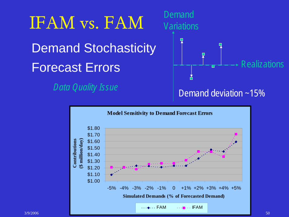
Realizations

DemandVariations

Demand deviation ~15%

IFAM vs. FAMDemand StochasticityForecast Errors

Data Quality Issue

Model Sensitivity to Demand Forecast Errors

$1.00$1.10$1.20$1.30$1.40$1.50$1.60$1.70$1.80

-5% -4% -3% -2% -1% 0 +1% +2% +3% +4% +5%Simulated Demands (% of Forecasted Demand)

Con

trib

utio

ns($

mill

ion/

day)

FAM IFAM

3/9/2006 16.75 51

Extending Fleet Assignment Models to Include “Incremental”

Schedule Design…

3/9/2006 16.75 52

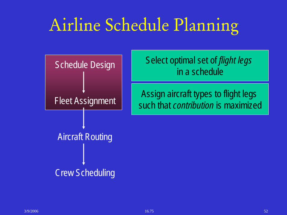
Airline Schedule Planning

Select optimal set of flight legsin a schedule

Schedule Design

Fleet AssignmentAssign aircraft types to flight legs

such that contribution is maximized

Aircraft Routing

Crew Scheduling

3/9/2006 16.75 53

Schedule Design: Fixed Flight Network, Flexible Schedule

Approach• Fleet assignment model with time

windows– Allows flights to be re-timed slightly (plus/

minus 10 minutes) to allow for improved utilization of aircraft and improved capacity assignments

Initial step in integrating flight schedule design and fleet assignment decisions

3/9/2006 16.75 54

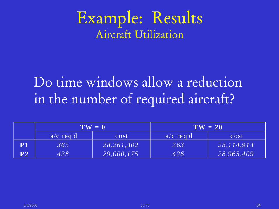
Example: ResultsAircraft Utilization

Do time windows allow a reduction in the number of required aircraft?

TW = 0 TW = 20a/c req'd cost a/c req'd cost

P1 365 28,261,302 363 28,114,913P2 428 29,000,175 426 28,965,409

3/9/2006 16.75 55

Results

• Time windows can provide significant cost savings, as well as a potential for freeing aircraft– $50 million in operating costs alone for one

U.S. airline

3/9/2006 16.75 56

Schedule Design: Optional Flights, Flexible Schedule

Approach• Fleet assignment with “optional” flight

legs– Additional flight legs representing varying

flight departure times– Additional flight legs representing new flights– Option to eliminate existing flights from

future flight network

Incremental Schedule Design

3/9/2006 16.75 57

Demand and Supply Interactions

A BMarket Share450

A B

100150100100

Market Share410

A BMarket Share300

100200

40100190

120

150

Non-LinearInteractions

3/9/2006 16.75 58

Formulation

Kk ∈∀

∑ ∑∑ ∑∈ ∈∈ ∈

−+Pp Pr

rpr

rpp

Kk Liikik tfarebfarefcMin )(~

,,

1, =∑∈ Kk

ikf

0),,(

,,,),,(

,,, =−−+ ∑∑∈∈

+−

tokOiiktok

tokIiiktok fyfy

kkCLi

ikOo

tok Nfyn

≤+ ∑∑∈∈ )(

,,,

{ }1,0, ∈ikf 0,, ≥toky

Fi L∀ ∈

tok ,,∀

S u b j e c t t o :

iPr Pp

rp

rp

pi

Pr Pp

rp

pi

kkik QtbtSEATSf ≥−+ ∑ ∑∑ ∑∑

∈ ∈∈ ∈δδ,

pPr

rp Dt ≤∑

∈

0≥rpt

Li ∈∀

Pp ∈∀

, 1k ik K

f∈

≤∑ Oi L∀ ∈

Kk ∈∀

∑ ∑∑ ∑∈ ∈∈ ∈

−+Pp Pr

rpr

rpp

Kk Liikik tfarebfarefcMin )(~

,,

1, =∑∈ Kk

ikf

0),,(

,,,),,(

,,, =−−+ ∑∑∈∈

+−

tokOiiktok

tokIiiktok fyfy

kkCLi

ikOo

tok Nfyn

≤+ ∑∑∈∈ )(

,,,

{ }1,0, ∈ikf 0,, ≥toky

Fi L∀ ∈

tok ,,∀

S u b j e c t t o :

iPr Pp

rp

rp

pi

Pr Pp

rp

pi

kkik QtbtSEATSf ≥−+ ∑ ∑∑ ∑∑

∈ ∈∈ ∈δδ,

pPr

rp Dt ≤∑

∈

0≥rpt

Li ∈∀

Pp ∈∀

, 1k ik K

f∈

≤∑ Oi L∀ ∈Flight SelectionFlight Selection

FAMFAMPMMPMM

Fleet AssignmentFleet AssignmentSpill + RecaptureSpill + Recapture

Schedule DesignSchedule Design

Lohatepanont, M. and Barnhart, Cynthia, “Airline Schedule Planning: Integrated Models and Algorithms for Schedule Design and Fleet Assignment,” Transportation Science, future.

3/9/2006 16.75 59

Schedule Design: Results• Demand and supply interactions

– Tractability potentially a big issue• Resulting schedules operate fewer flights

– Lower operating costs– Fewer aircraft required

• Order of magnitude impact: ~$100 - $350 million improvement annually for variable market demand– Rough estimates: sensitive to quality of data, spill and

recapture assumptions, demand forecasts and stochasticity

– Comparison to planners’ schedules– Excludes benefits from saved aircraft