Group members

Muhammad Bilal (11-EE-074)

Waheed Ashfaq (11-EE-140)

Farhaj Ishtiaq ch. (11-EE-031)

HITEC UNIVERSITY TAXILA CANTT PAKISTAN(DEPARTMENT OF ELECTRICAL ENGINEERING)

TOPIC

Aircraft Pitch

CONTENTS:

Aircraft Pitch System Modeling

Aircraft Pitch System Analysis

Aircraft Pitch PID Controller Design

Aircraft Pitch Root Locus Controller Design

Aircraft Pitch Simulink Modeling

What is pitch angle and angle of attack in

air-craft

Pitch angle: is the angle between the center line of the roll axis of the aircraft (nose to tail, the longitudinal axis) and the horizon.

Angle of attack is the angle between the chord line of an airfoil and the relative wind through which it is moving.

The angle of attack and the pitch angle are usually different in flights

Sometimes the pitch angle may be positive or negative in normal flight, but the angle of attack is always positive.

Principle of flight

There are 4 forces involved with flight:i. Lift

ii. Weight

iii. Thrust

iv. Drag

AXIS OF FLIGHT

Three axis’ of flight include:Pitch, Roll, and Yaw

1. Pitch is controlled by the air flow across the elevators.

1. Yaw is controlled by the air flow across the rudder

1. Roll is controlled by the air flow across the ailerons

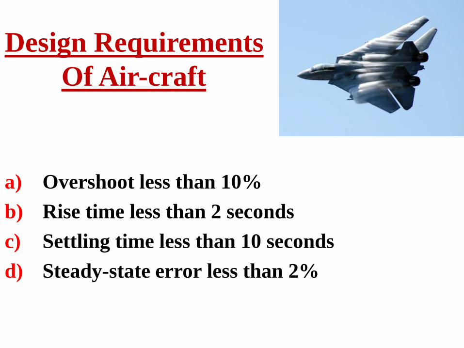
Design Requirements

Of Air-craft

a) Overshoot less than 10%

b) Rise time less than 2 seconds

c) Settling time less than 10 seconds

d) Steady-state error less than 2%

Aircraft Pitch: System Modeling

System Modeling

• The of equations governing the motion of an aircraft are a very complicated set of six nonlinear coupled differential equations.

• However, under certain assumptions, they can be decoupled and linearized into longitudinal and lateral equations. Aircraft pitch is governed by the longitudinal dynamics. In this example we will design an autopilot that controls the pitch of an aircraft.

Conti……

We will assume that the aircraft is in steady-state at

constant altitude and velocity.

Thus, the thrust, drag, weight and lift forces balance each

other in the x- and y-directions.

We will also assume that a change in pitch angle will not

change the speed of the aircraft under any circumstance

(unrealistic but simplifies the problem a bit).

Under these assumptions, the longitudinal equations of

motion for the aircraft can be written as follows:

Transfer Function:

Before finding the transfer function and state-space models,

let's plug in some numerical values to simplify the modeling

equations shown above:

Above equation become:

Transfer Function:

To find the transfer function of the above system, we need to take the Laplace transform of the above modeling equations.

The Laplace transform of the above equations are shown below.

MATLAB

Representation:

Output:

Aircraft Pitch: System

Analysis

System analysis contain:

Open loop response.

Close loop response.

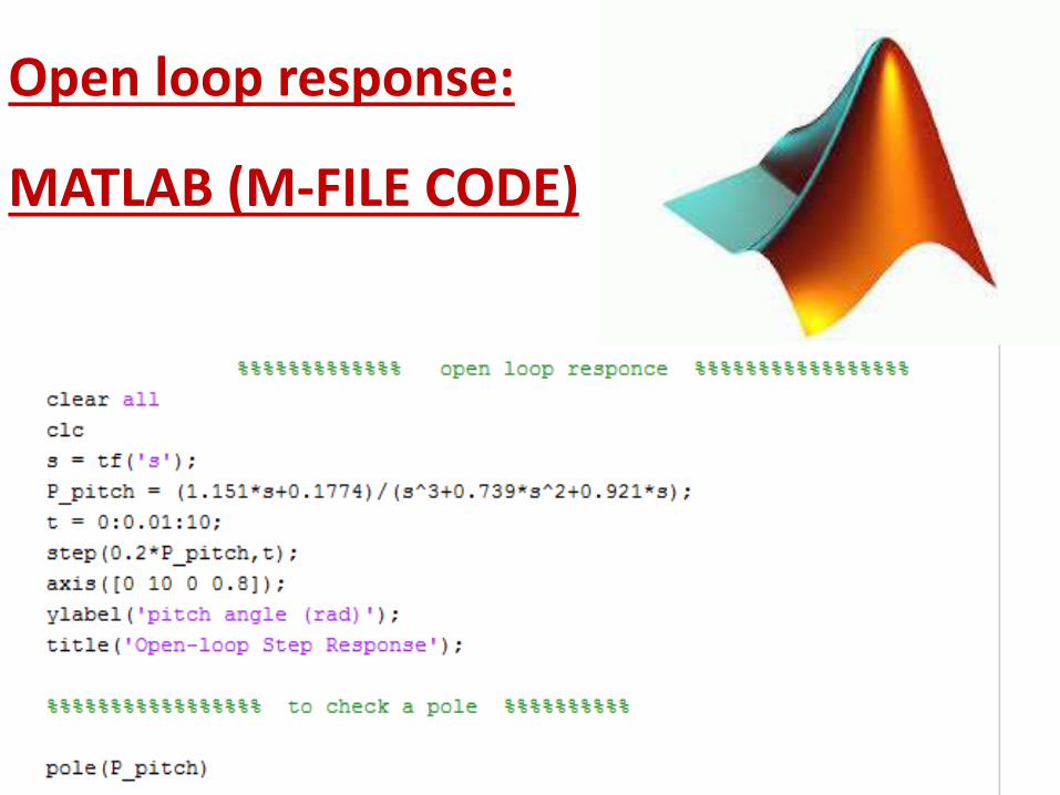
Open loop response:

MATLAB (M-FILE CODE)

Output:

From the above plot, we see that the open-loop response does not satisfy the design criteria at all. In fact, the open-loop response is unstable.

Stability of a system can be determined by examining the poles of the transfer function where the poles can be identified using the MATLAB command pole as shown below.

Pole(P_pitch)

As indicated by this function, one of the poles of the open-loop transfer function is on the imaginary axis while the other two poles are in the left-half of the complex s-plane.

A pole on the imaginary axis indicates that the free response of the system will not grow unbounded, but also will not decay to zero. Even though the free response will not grow unbounded.

Closed-loop response:

In order to stabilize this system and eventually meet our given design requirements, we will add a feedback controller.

Closed loop code:

OUTPUT

conti…..

The above plot again demonstrates that this closed-loop system does not meet the given design requirements.

Aircraft Pitch:

PID Controller Design

PID Controller Design

In PID controller design we cover:

• Proportional control

• PI control

• PID Control

1. In PID controller designing we use SISO tool.

2. The main advantage of using the SISO tool Design within MATLAB is that it have the automated tuning capabilities which design the PID controller

Design Criteria For PID:

Proportional control

Let's begin by designing a proportional controller of the form C(s) = Kp. The SISO Design Tool we will use for design can be opened by typing SISOtool(P_pitch) at the command line.

This will open both the SISO Design Task window as well as the Control and Estimation Tools Manager window.

Since our reference is a step function of 0.2 radians, we can set the precompensator block F(s) equal to 0.2 to scale a unit step input to our system.

This can be accomplished from the Compensator Editor tab of the open window. Specifically, choose F from the drop-down menu in the Compensator portion of the window and set the compensator equal to 0.2 as shown in the figure below

To see the performance of our system with this controller, go to the Analysis Plots tab of the Control and Estimation Tools Manager window.

Then choose a Plot Type of Step for Plot 1 in the Analysis Plots section of the window as shown below. Then choose a response of Closed loop r to y for Plot 1 as shown in the figure below:

The resulting performance is improved, though the settle time is still much too large. We will likely need to add integral and/or derivative terms to our controller in order to meet the given requirements.

PI control

From inspection of the above, notice that the addition of integral control helped reduce the average error in the signal more quickly.

Unfortunately, the integral control also made the response more oscillatory, therefore, the settle time requirement is still not met.

the overshoot requirement is no longer met either. Let's try also adding a derivative term to our controller

PID Control

Increasing the derivative gain Kd in a PID controller can often help reduce overshoot.

Therefore, by adding derivative control we may be able to reduce the oscillation in the response a sufficient amount that we can then increase the other gains to reduce the settling time.

Let's test our hypothesis by changing the Controller type to PID and again clicking the Update Compensator button. The generated controller is shown below.

Output of PID:

Conti…….

The response shown above meets all of the given requirements as summarized below.

Overshoot = 5% < 10%

Rise time = 1.2 seconds < 2 seconds

Settling time = 5 seconds < 10 seconds

Steady-state error = 0% < 2%

Therefore, this PID controller will provide the desired performance of the aircraft's pitch.

Aircraft Pitch: Root Locus Controller Design

M-File Code For Root Locus:

Root Locus Plot:

Root-Locus plot:

Output Of Root Locus:

This diagram meets all the requirements which we needed except settling time which we required 10sec but here it is 35.1sec

Conti…..

In order to get the required criteria we move the pink boxes on the root locus and dragging the box along the locus in the direction of increasing K.

The step response plot will automatically update

The effect of increasing K to a value of 200 will be that the two slowest closed-loop poles will approach closed-loop zeros thereby making their effect minimal

Conti….

A loop gain of K = 200 keeps all of the poles on the real-axis, leading to no overshoot and the presence of the integrator in the plant guarantees zero steady-state error.

Therefore, this controller meets all of the given requirements as shown in the figure below.

Our Required Outputwhen K=200

Aircraft Pitch: Simulink Modeling

In Simulink Model contains:

Building the state-space model

Generating the open-loop and closed-loop response

State-Space Model

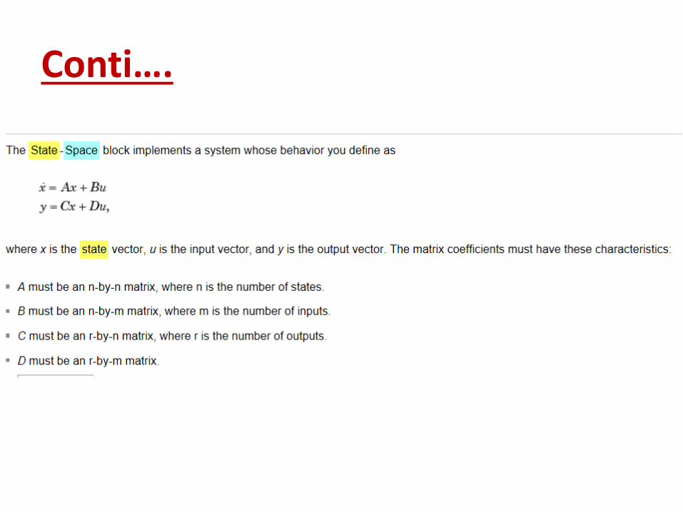
Conti….

Simulink models:

Open-loop response:

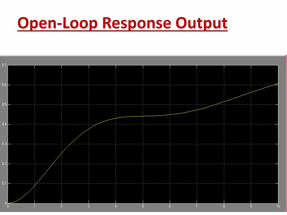
Open-Loop Response Output

Conti…..

This response is unstable and identical to that obtained in the Aircraft Pitch: System Analysis.

In order to view a stable response, we will now quickly add the state-feedback control gain K.

When gain of K is added our new Simulink diagram of open-loop response becomes…….

Simulink modelclosed-loop response:

Closed-Loop Response Output

Conti…

The output of closed-loop response is similar to Aircraft Pitch: State-Space Methods for Controller Design.

Where the state-feedback controller was designed.