
ADVANCED TECHNIQUES FOR CLOSED-LOOP …qc661yn3508/PhDthesis_main...ADVANCED TECHNIQUES FOR...
195
ADVANCED TECHNIQUES FOR CLOSED-LOOP RESERVOIR OPTIMIZATION UNDER UNCERTAINTY A DISSERTATION SUBMITTED TO THE DEPARTMENT OF ENERGY RESOURCES ENGINEERING AND THE COMMITTEE ON GRADUATE STUDIES OF STANFORD UNIVERSITY IN PARTIAL FULFILLMENT OF THE REQUIREMENTS FOR THE DEGREE OF DOCTOR OF PHILOSOPHY Mehrdad Gharib Shirangi April 2017
Transcript of ADVANCED TECHNIQUES FOR CLOSED-LOOP …qc661yn3508/PhDthesis_main...ADVANCED TECHNIQUES FOR...

ADVANCED TECHNIQUES FOR CLOSED-LOOP RESERVOIR
OPTIMIZATION UNDER UNCERTAINTY
A DISSERTATION
SUBMITTED TO THE DEPARTMENT OF
ENERGY RESOURCES ENGINEERING
AND THE COMMITTEE ON GRADUATE STUDIES
OF STANFORD UNIVERSITY
IN PARTIAL FULFILLMENT OF THE REQUIREMENTS
FOR THE DEGREE OF
DOCTOR OF PHILOSOPHY
Mehrdad Gharib Shirangi
April 2017

http://creativecommons.org/licenses/by-nc/3.0/us/
This dissertation is online at: http://purl.stanford.edu/qc661yn3508
© 2017 by Mehrdad Gharib Shirangi. All Rights Reserved.
Re-distributed by Stanford University under license with the author.
This work is licensed under a Creative Commons Attribution-Noncommercial 3.0 United States License.
ii

I certify that I have read this dissertation and that, in my opinion, it is fully adequatein scope and quality as a dissertation for the degree of Doctor of Philosophy.
Louis Durlofsky, Primary Adviser
I certify that I have read this dissertation and that, in my opinion, it is fully adequatein scope and quality as a dissertation for the degree of Doctor of Philosophy.
Tapan Mukerji
I certify that I have read this dissertation and that, in my opinion, it is fully adequatein scope and quality as a dissertation for the degree of Doctor of Philosophy.
Oleg Volkov
Approved for the Stanford University Committee on Graduate Studies.
Patricia J. Gumport, Vice Provost for Graduate Education
This signature page was generated electronically upon submission of this dissertation in electronic format. An original signed hard copy of the signature page is on file inUniversity Archives.
iii

iv

To the memory of my grandfather
Seyed Khalil Hosseini Ghasemi (1933-2015)
v

vi
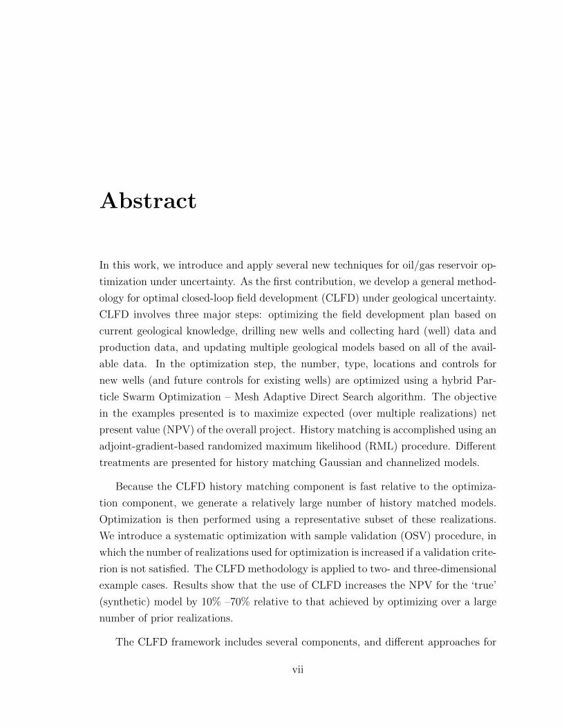
Abstract
In this work, we introduce and apply several new techniques for oil/gas reservoir op-
timization under uncertainty. As the first contribution, we develop a general method-
ology for optimal closed-loop field development (CLFD) under geological uncertainty.
CLFD involves three major steps: optimizing the field development plan based on
current geological knowledge, drilling new wells and collecting hard (well) data and
production data, and updating multiple geological models based on all of the avail-
able data. In the optimization step, the number, type, locations and controls for
new wells (and future controls for existing wells) are optimized using a hybrid Par-
ticle Swarm Optimization – Mesh Adaptive Direct Search algorithm. The objective
in the examples presented is to maximize expected (over multiple realizations) net
present value (NPV) of the overall project. History matching is accomplished using an
adjoint-gradient-based randomized maximum likelihood (RML) procedure. Different
treatments are presented for history matching Gaussian and channelized models.
Because the CLFD history matching component is fast relative to the optimiza-
tion component, we generate a relatively large number of history matched models.
Optimization is then performed using a representative subset of these realizations.
We introduce a systematic optimization with sample validation (OSV) procedure, in
which the number of realizations used for optimization is increased if a validation crite-
rion is not satisfied. The CLFD methodology is applied to two- and three-dimensional
example cases. Results show that the use of CLFD increases the NPV for the ‘true’
(synthetic) model by 10% –70% relative to that achieved by optimizing over a large
number of prior realizations.
The CLFD framework includes several components, and different approaches for
vii
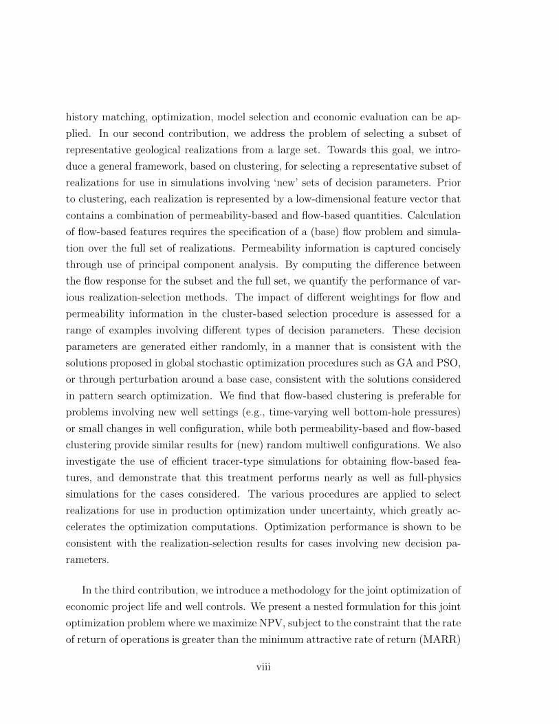
history matching, optimization, model selection and economic evaluation can be ap-
plied. In our second contribution, we address the problem of selecting a subset of
representative geological realizations from a large set. Towards this goal, we intro-
duce a general framework, based on clustering, for selecting a representative subset of
realizations for use in simulations involving ‘new’ sets of decision parameters. Prior
to clustering, each realization is represented by a low-dimensional feature vector that
contains a combination of permeability-based and flow-based quantities. Calculation
of flow-based features requires the specification of a (base) flow problem and simula-
tion over the full set of realizations. Permeability information is captured concisely
through use of principal component analysis. By computing the difference between
the flow response for the subset and the full set, we quantify the performance of var-
ious realization-selection methods. The impact of different weightings for flow and
permeability information in the cluster-based selection procedure is assessed for a
range of examples involving different types of decision parameters. These decision
parameters are generated either randomly, in a manner that is consistent with the
solutions proposed in global stochastic optimization procedures such as GA and PSO,
or through perturbation around a base case, consistent with the solutions considered
in pattern search optimization. We find that flow-based clustering is preferable for
problems involving new well settings (e.g., time-varying well bottom-hole pressures)
or small changes in well configuration, while both permeability-based and flow-based
clustering provide similar results for (new) random multiwell configurations. We also
investigate the use of efficient tracer-type simulations for obtaining flow-based fea-
tures, and demonstrate that this treatment performs nearly as well as full-physics
simulations for the cases considered. The various procedures are applied to select
realizations for use in production optimization under uncertainty, which greatly ac-
celerates the optimization computations. Optimization performance is shown to be
consistent with the realization-selection results for cases involving new decision pa-
rameters.
In the third contribution, we introduce a methodology for the joint optimization of
economic project life and well controls. We present a nested formulation for this joint
optimization problem where we maximize NPV, subject to the constraint that the rate
of return of operations is greater than the minimum attractive rate of return (MARR)
viii

or hurdle rate. The methodology provides the optimal project life and the optimal
well controls such that the maximum NPV is obtained at the end of the project
life, and the rate of return of the project is essentially equal to MARR. Application
of this procedure, enables avoiding situations where NPV increases slowly in time,
but the benefit relative to the capital employed is extremely low. We demonstrate
the successful application of this treatment for production optimization for two- and
three-dimensional reservoir models.
ix

x

Acknowledgments
First and foremost, I would like to thank God who has always helped and guided me
throughout my life and academic career.
I would like to express my sincere appreciation to my adviser, Prof. Louis Durlof-
sky, for his incredible support, patience, guidance and encouragement throughout my
PhD study. Working with him has been a wonderful journey to learn and grow in
many ways, including research and communication skills, critical thinking, concise
and coherent writing, and professionalism. I am particularly indebted to him for his
confidence in me and for providing me the freedom and opportunity to pursue some
of my own ideas, while watching over my progress and directing the research towards
a coherent set of contributions. I consider myself very fortunate for having him as
my PhD adviser. I also would like to thank Dr. Oleg Volkov for his help during
my PhD, and for serving on my PhD committee. My acknowledgements extend to
Profs. Tapan Mukerji, Roland Horne, and Peter Kitanidis for serving on my defense
committee.
I would like to extend my thanks to all other faculty and staff in the Energy
Resources Engineering Department. In particular, I want to thank Profs. Khalid
Aziz, Hamdi Tchelepi, Jef Caers, Anthony Kovscek, Kurt House and Marco Thiele,
with whom I have met on occasion for various discussions on research. I am grateful
to Dr. Obiajulu Isebor for providing the PSO-MADS code and for many useful dis-
cussions. Special thanks also to Profs. Carlo Alberto Magni (University of Modena),
Michael Saunders and Trevor Hastie (Stanford University), Jo Eidsvik (NTNU), Hadi
Hajibeygi and Denis Voskov (Delft University), Dr. David Echeverrıa Ciaurri (IBM),
and Drs. Mohammad Karimi-Fard and Celine Scheidt (Stanford University) for help-
ful discussions. I also thank Eiko Rutherford and Joanna Sun, our administrative
xi

associates, for their support on various occasions.
I would like to thank the industrial affiliates of the Stanford Smart Fields Con-
sortium for financial support, and the Stanford Center for Computational Earth &
Environmental Science (CEES) for providing the computational resources used in
this work. Special thanks to Dennis Michael who has always been of great help in
facilitating issues with CEES.
I have been fortunate to have great friends at Stanford University. I would like
to express my special thanks to my friends in the ERE department with whom I
had discussions about research, Jacob Englander, Mohammad S. Masnadi, Charles
Kang and Philip Brodrick. I would like to thank other friends in the ERE De-
partment, Yashar Mehmani, Sara Farshidi, Amir Salehi, Amir Delgoshaie, Moham-
mad Bazargan, Alireza Iranshahr, Mohammad Shahvali, Yongduk Shin, Elnur Aliyev,
Karine Levonyan, Julia Foster, Wen Song, Morgan Ames, Forest Jiang, Sumeet Tre-
han, Matthieu Rousset and Hai Vo. I also thank my Stanford friends outside the
department, Michael Albert, Long Do, Robert Shields, Rall Walsh, Ali Shariati, Ali
Shahmoradi and Asieh Tarami.
I want to thank my family who supported me during my PhD study. I especially
thank my little nephews Sajjad, Mohammad Arvin, and Ryan, whose presence gave
me hope and energy during the past years. I dedicate this dissertation to the memory
of my grandfather, Seyed Khalil Hosseini Ghasemi.
xii
Contents
Abstract vii
Acknowledgments xi
1 Introduction 1
1.1 Literature Review . . . . . . . . . . . . . . . . . . . . . . . . . . . . . 2
1.1.1 Optimization approaches for oil field operations . . . . . . . . 2
1.1.2 Optimization under uncertainty and selection of representative
models . . . . . . . . . . . . . . . . . . . . . . . . . . . . . . . 7
1.1.3 Economic measures for reservoir performance . . . . . . . . . 10
1.1.4 History matching of production data . . . . . . . . . . . . . . 11
1.1.5 Closed-loop reservoir management . . . . . . . . . . . . . . . . 12
1.2 Scope of Work . . . . . . . . . . . . . . . . . . . . . . . . . . . . . . . 14
1.3 Dissertation Outline . . . . . . . . . . . . . . . . . . . . . . . . . . . 17
2 Closed-Loop Field Development 19
2.1 CLFD workflow . . . . . . . . . . . . . . . . . . . . . . . . . . . . . . 19
2.2 CLFD optimization . . . . . . . . . . . . . . . . . . . . . . . . . . . . 22
2.3 Optimization with sample validation . . . . . . . . . . . . . . . . . . 25
2.4 CLFD history matching . . . . . . . . . . . . . . . . . . . . . . . . . 26
2.5 Computational results . . . . . . . . . . . . . . . . . . . . . . . . . . 29
2.5.1 Example 2.1: Simultaneous versus sequential optimization of
field development . . . . . . . . . . . . . . . . . . . . . . . . . 29
2.5.2 Example 2.2: CLFD for a two-dimensional reservoir model . . 33
2.5.3 Example 2.3: CLFD for a three-dimensional reservoir model . 49
xiii

2.6 Summary . . . . . . . . . . . . . . . . . . . . . . . . . . . . . . . . . 53
3 Selection of Representative Models 55
3.1 Assessment of flow-response statistics . . . . . . . . . . . . . . . . . . 56
3.2 Unsupervised Learning for Model Selection . . . . . . . . . . . . . . . 60
3.2.1 Feature selection . . . . . . . . . . . . . . . . . . . . . . . . . 60
3.2.2 Clustering for selection of representative realizations . . . . . . 64
3.3 Computational results . . . . . . . . . . . . . . . . . . . . . . . . . . 65
3.3.1 Example 3.1: new well settings in channelized models . . . . . 66
3.3.2 Example 3.2: new well configurations . . . . . . . . . . . . . . 74
3.3.3 Summary of realization-selection results . . . . . . . . . . . . 80
3.4 production optimization under uncertainty . . . . . . . . . . . . . . . 83
3.4.1 Optimization of well controls with representative realizations . 83
3.4.2 Example 3.3: production optimization under uncertainty . . . 85
3.4.3 Additional observations . . . . . . . . . . . . . . . . . . . . . . 88
3.4.4 Summary . . . . . . . . . . . . . . . . . . . . . . . . . . . . . 89
4 Optimization of Economic Project Life 91
4.1 Economic measures and production optimization . . . . . . . . . . . . 92
4.1.1 Net present value computation . . . . . . . . . . . . . . . . . . 92
4.1.2 Modified internal rate of return and economic project life . . . 93
4.1.3 Optimization problem statement . . . . . . . . . . . . . . . . 96
4.2 Computational results . . . . . . . . . . . . . . . . . . . . . . . . . . 98
4.2.1 Example 4.1: 2D bimodal reservoir . . . . . . . . . . . . . . . 98
4.2.2 Example 4.2: 3D binary reservoir . . . . . . . . . . . . . . . . 111
4.3 Summary . . . . . . . . . . . . . . . . . . . . . . . . . . . . . . . . . 115
5 Summary, Conclusions and Future Work 117
5.1 Conclusions . . . . . . . . . . . . . . . . . . . . . . . . . . . . . . . . 117
5.2 Future work . . . . . . . . . . . . . . . . . . . . . . . . . . . . . . . . 120
Nomenclature 123
Bibliography 127
xiv
Appendices 145
A CLFD for Channelized Models 147
A.1 History matching for channelized models . . . . . . . . . . . . . . . . 147
A.2 Example A1: CLFD for a channelized model . . . . . . . . . . . . . . 149
B Representative Models for a Binary System 157
B.1 Example B1: new well settings . . . . . . . . . . . . . . . . . . . . . . 157
B.1.1 Representative realizations for random well controls . . . . . . 158
B.1.2 Representative realizations for small changes in well controls . 159
B.2 Example B2: new well configurations . . . . . . . . . . . . . . . . . . 161
B.2.1 Representative realizations for random well configurations . . 162
B.2.2 Representative realizations for small changes in well locations 163
B.2.3 Summary of realization-selection results . . . . . . . . . . . . 166
xv

xvi

List of Tables
2.1 Optimization parameters for all examples . . . . . . . . . . . . . . . . 31
2.2 Final NPVs ($ MM) for three runs for sequential (well-by-well) and
simultaneous optimization (Example 2.1) . . . . . . . . . . . . . . . . 32
2.3 NPV values ($ MM) from optimization over 50 prior realizations and
from CLFD optimization, for three different true models (Example 2.2) 45
2.4 Initial and final numbers of representative realizations (determined us-
ing OSV) and the corresponding relative improvement values at each
CLFD step (Example 2.3) . . . . . . . . . . . . . . . . . . . . . . . . 52
3.1 Median (mD) values of Dα=0, Dα=0.5, Dα=1 and Drand, for 100 random
well control vectors, for different nr. Average mD values and average
ranking are also provided (Example 3.1). . . . . . . . . . . . . . . . . 69
3.2 Median values (mD) of Dα=0,prx and Dα=0.5,prx for 100 random well
control vectors, for different nr. Average mD values are also provided
(Example 3.1). . . . . . . . . . . . . . . . . . . . . . . . . . . . . . . 71
3.3 Results for various permeability-based clustering treatments (α = 1 in
all cases). Median (mD) values of Dl=99, Dfull PCA and Dfull perm, for
100 random well control vectors, for different nr. Average mD values
are also provided (Example 3.1). . . . . . . . . . . . . . . . . . . . . . 72
3.4 Results using k-medoids clustering. Median (mD) values of Dα=0,
Dα=0.5 and Dα=1, for 100 random well control vectors, for different
nr. Last column shows computational time for selection with α = 0.
Average values are also provided (Example 3.1). . . . . . . . . . . . . 73
xvii

3.5 Median (mD) values of Dα=0, Dα=0.5 and Dα=1, for 100 well control
vectors corresponding to pattern search mesh points, for different nr.
Average mD values and average ranking are also provided (Example 3.1). 75
3.6 Median values (mD) of Dα=0,prx and Dα=0.5,prx for 100 well control
vectors corresponding to pattern search mesh points, for different nr.
Average mD values are also provided (Example 3.1). . . . . . . . . . 75
3.7 Median (mD) values of Dα=0, Dα=0.5, Dα=1 and Drand, for 100 random
well configurations, for different nr. Average mD values and average
ranking are also provided (Example 3.2). . . . . . . . . . . . . . . . 77
3.8 Median values (mD) of Dα=0,prx and Dα=0.5,prx for 100 random well
configurations, for different nr. Average mD values are also provided
(Example 3.2). . . . . . . . . . . . . . . . . . . . . . . . . . . . . . . 78
3.9 Median (mD) values of Dα=0, Dα=0.5 and Dα=1, for 40 well configu-
rations corresponding to pattern search mesh points, for different nr.
Average mD values and average ranking are also provided (Example 3.2). 81
3.10 Median values (mD) ofDα=0,prx andDα=0.5,prx for 40 well configurations
corresponding to pattern search mesh points, for different nr. Average
mD values are also provided (Example 3.2). . . . . . . . . . . . . . . 81
3.11 Summary of results: average mD values for nr = 3, . . . , 15 for all cases.
The smallest value for each case is indicated in bold. . . . . . . . . . 83
3.12 Economic parameters and bounds for Example 3.3 . . . . . . . . . . . 85
3.13 Improvement in expected objective (in $106) for the full set of 200
realizations, J(xopt,Mfull)− J(x0,Mfull), evaluated using xopt obtained
from optimization runs with nr = 3 (Example 3.3). . . . . . . . . . . 87
3.14 Improvement in expected objective (in $106) for the full set of 200
realizations, J(xopt,Mfull)− J(x0,Mfull), evaluated using xopt obtained
from optimization runs with nr = 6 (Example 3.3). . . . . . . . . . . 88
4.1 Economic parameters and BHP ranges for all examples . . . . . . . . 100
4.2 NPV ($ MM), corresponding MIRR and fluid production/injection
(MM STB) for optimal controls with different project life. The so-
lution with T ∗ = 2340 days represents an optimum (Example 4.1). . . 105
xviii

4.3 Optimal NPV, corresponding MIRR and fluid production/injection
(MM STB) from optimal controls with different initial-guess BHPs
with T = 2340 days (Example 4.1). . . . . . . . . . . . . . . . . . . . 108
4.4 Optimal NPV and the corresponding MIRR for different (specified)
project life (Example 4.1). . . . . . . . . . . . . . . . . . . . . . . . . 109
4.5 Optimal NPV and the corresponding MIRR and EPL (T ∗) from opti-
mizations with different discount rates (Example 4.1). . . . . . . . . . 110
A.1 NPV values ($ MM) from optimization over prior realizations with nr =
5 and by use of OSV (where nr is increased to satisfy RI > 0.5) and
from CLFD by use of OSV, for five different true models (Example A1) 156
A.2 NPV values ($ MM) from optimization over prior realizations by use
of OSV (where nr is increased to satisfy RI > 0.5) and from CLFD by
use of OSV, for true model 4 (Example A1) . . . . . . . . . . . . . . 156
B.1 Median values (mD) of Dα=0, Dα=0.5, Dα=1 and Drand, for 300 random
well control vectors, for different nr. Average mD values and average
ranking are also provided (Example B1). . . . . . . . . . . . . . . . 160
B.2 Median (mD) values of Dα=0, Dα=0.5 and Dα=1, for 126 well control
vectors corresponding to pattern search mesh points, for different nr.
Average mD values and average ranking are also provided (Example B1).162
B.3 Median (mD) values of Dα=0, Dα=0.5, Dα=1 and Drand, for 300 random
well configurations, for different nr. Average mD values and average
ranking are also provided (Example B2). . . . . . . . . . . . . . . . . 164
B.4 Median (mD) values of Dα=0, Dα=0.5 and Dα=1, for 40 well configu-
rations corresponding to pattern search mesh points, for different nr.
Average mD values and average ranking are also provided (Example B2).165
B.5 Summary of results: average mD values for nr = 3, . . . , 15 for all cases.
The smallest value for each case is indicated in bold. . . . . . . . . . 166
xix

xx

List of Figures
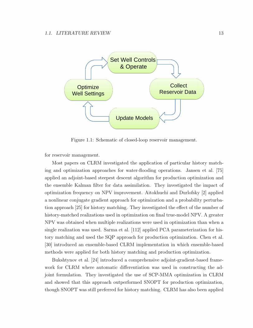
1.1 Schematic of closed-loop reservoir management. . . . . . . . . . . . . 13
1.2 Schematic of closed-loop field development (CLFD). . . . . . . . . . . 14
2.1 Schematic and notation for the closed-loop field development optimiza-
tion procedure. . . . . . . . . . . . . . . . . . . . . . . . . . . . . . . 22
2.2 True log-permeability field for Examples 2.1 and 2.2. Permeability is
in mD. . . . . . . . . . . . . . . . . . . . . . . . . . . . . . . . . . . . 30
2.3 Oil and water relative permeability curves for Example 2.1. . . . . . 31
2.4 Final oil saturation (at 3000 days) from optimal solutions for the two
approaches (Example 2.1). Well locations are also shown, with red
denoting producer, blue denoting injector, and the well numbers indi-
cating the drilling sequence. . . . . . . . . . . . . . . . . . . . . . . . 33
2.5 Oil and water relative permeability curves for Examples 2 and 3. . . 34
2.6 Well configuration from deterministic optimization (using mtrue), with
red denoting producer, blue denoting injector, and the well numbers
indicating the drilling sequence. Background shows final oil saturation
(Example 2.2). . . . . . . . . . . . . . . . . . . . . . . . . . . . . . . 36
2.7 Ordered NPV plot for NR = 50 prior realizations based on initial guess
for decision variables x0. The three selected realizations are shown in
red (Example 2.2, nr = 3). . . . . . . . . . . . . . . . . . . . . . . . . 37
2.8 Three representative prior realizations of log-permeability, along with
the initial-guess well configuration (Example 2.2). Red (outlined) cir-
cles denote producers, blue injectors, and the well numbers indicate
the drilling sequence. . . . . . . . . . . . . . . . . . . . . . . . . . . . 37
xxi
2.9 Evolution of expected NPV (J(x,M1rep)) for optimization over nr = 3
prior realizations (Example 2.2). . . . . . . . . . . . . . . . . . . . . . 38
2.10 Optimal well configuration and drilling sequence at t1 and t2. Solid red
and blue circles denote producers and injectors (drilled or in the process
of being drilled), and outlined red and blue circles denote planned
producers and injectors. Numbers indicate the drilling sequence and
background shows log-permeability for one realization (Example 2.2,
nr = 3). . . . . . . . . . . . . . . . . . . . . . . . . . . . . . . . . . . 39
2.11 Optimal expected NPV, J(xi,M irep), and the expected NPV for the
corresponding initial guess, J(xi−1,M irep), versus CLFD step (Exam-
ple 2.2, nr = 3). . . . . . . . . . . . . . . . . . . . . . . . . . . . . . . 40
2.12 Optimal expected NPV, J(xi,M irep), and the corresponding NPV for
the true model, J(xi,mtrue), versus CLFD step. The star shows the
final true NPV from CLFD (Example 2.2, nr = 3). . . . . . . . . . . 40
2.13 NPV for the nr = 3 (representative) realizations, and the correspond-
ing NPV for the true model, versus CLFD step (Example 2.2). . . . . 42
2.14 Optimal expected NPV, and the corresponding NPV for the true model,
versus CLFD step, for different numbers of representative realizations.
The star shows the final true NPV from CLFD (Example 2.2). . . . . 44
2.15 NPV for different numbers of representative realizations, and the cor-
responding NPV for the true model, versus CLFD step (Example 2.2). 45
2.16 P10, P50, P90 NPVs evaluated for the entire set of 50 realizations,
along with the expected NPV for the representative set, versus CLFD
step (Example 2.2). . . . . . . . . . . . . . . . . . . . . . . . . . . . . 46
2.17 Optimal expected NPV, and the corresponding NPV for the true model,
versus CLFD step. The number of realizations at each CLFD step is
determined using OSV. The star shows the final true NPV from CLFD
(Example 2.2). . . . . . . . . . . . . . . . . . . . . . . . . . . . . . . 47
xxii

2.18 Evolution of two RML realizations (log-permeability is shown) for dif-
ferent CLFD steps. Current optimal well configuration and drilling
sequence is also depicted. Solid red and blue circles denote producers
and injectors (drilled or in the process of being drilled), and outlined
red and blue circles denote planned producers and injectors. Numbers
indicate the drilling sequence (Example 2.2). . . . . . . . . . . . . . . 48
2.19 True log-permeability field with initial guess for well configuration,
which includes three horizontal producers and three vertical injectors
(Example 2.3). . . . . . . . . . . . . . . . . . . . . . . . . . . . . . . 50
2.20 Optimal expected NPV, and the corresponding NPV for the true model,
versus CLFD step. The number of realizations at each CLFD step is
determined using OSV. The star shows the final true NPV from CLFD
(Example 2.3). . . . . . . . . . . . . . . . . . . . . . . . . . . . . . . 51
2.21 Final optimal solution from CLFD with OSV. Horizontal producers
are shown in red and vertical injectors in blue (Example 2.3). . . . . . 53
3.1 Illustration of some of the components of qkj (for well k = 1). The
reservoir life is 3000 days, which is divided into nt = 3 intervals. . . . 57
3.2 Oil and water relative permeability curves for all examples. . . . . . . 66
3.3 Three conditional realizations of log-permeability field for bimodal
channelized model. Fixed well configuration is also shown – circles
denote producers and triangles indicate injectors (Examples 3.1 and
3.3). . . . . . . . . . . . . . . . . . . . . . . . . . . . . . . . . . . . . 67
3.4 Injector BHP profiles corresponding to a random well-control vector
xnew (Example 3.1). . . . . . . . . . . . . . . . . . . . . . . . . . . . . 68
3.5 Box plots of Dα=0, Dα=0.5 and Dα=1 for 100 random well control vec-
tors. The red line within each box corresponds to the median, and
the bottom and top of each box correspond to the 25th and 75th per-
centiles. The lines above and below the boxes correspond to the 2nd
and 98th percentiles (Example 3.1). . . . . . . . . . . . . . . . . . . . 70
xxiii
3.6 Box plots of Dα=0, Dα=0.5 and Dα=1 for 100 well control vectors corre-
sponding to pattern search mesh points. The red line within each box
corresponds to the median, and the bottom and top of each box cor-
respond to the 25th and 75th percentiles. The lines above and below
the boxes correspond to the 2nd and 98th percentiles (Example 3.1). 74
3.7 Three realizations of log-permeability field and three base well config-
urations for computing flow-based features used in clustering. Circles
denote producers and triangles indicate injectors (Example 3.2). . . . 75
3.8 Three (out of 100) random well configurations, xnew, for computing flow
responses. Circles indicate producers and triangles denote injectors
(Example 3.2). . . . . . . . . . . . . . . . . . . . . . . . . . . . . . . 76
3.9 Box plots of Dα=0, Dα=0.5 and Dα=1 for 100 random well configura-
tions. The red line within each box corresponds to the median, and
the bottom and top of each box correspond to the 25th and 75th per-
centiles. The lines above and below the boxes correspond to the 2nd
and 98th percentiles (Example 3.2). . . . . . . . . . . . . . . . . . . . 78
3.10 Base-case well configuration, and two (out of 40) new well configu-
rations corresponding to pattern search mesh points. Circles denote
producers and triangles indicate injectors (Example 3.2). . . . . . . . 79
3.11 Box plots of Dα=0, Dα=0.5 and Dα=1 for 40 well configurations corre-
sponding to pattern search mesh points. The red line within each box
corresponds to the median, and the bottom and top of each box cor-
respond to the 25th and 75th percentiles. The lines above and below
the boxes correspond to the 2nd and 98th percentiles (Example 3.2). 80
4.1 Example cash flow stream for a production optimization problem. Cash
flows are computed for each 90-day control step. . . . . . . . . . . . . 95
4.2 MIRR trajectory corresponding to cash flow stream in Fig. 4.1. The
dashed vertical line shows the time where the rate of return becomes
smaller than the specified MARR of 0.15. . . . . . . . . . . . . . . . . 96
4.3 Log-permeability field with well locations. Circles denote producers
and triangles denote injectors (Example 4.1). . . . . . . . . . . . . . . 99
xxiv
4.4 NPV trajectory from inner optimization with (a) initial guess T , and
(b) T for which NPV in (a) is the maximum. The dashed vertical line in
(a) shows the time where the maximum NPV is obtained (Example 4.1).101
4.5 Cash flow stream for the optimal controls with T = 3240 days (Exam-
ple 4.1). . . . . . . . . . . . . . . . . . . . . . . . . . . . . . . . . . . 102
4.6 (a) Cash flow percentage, computed yearly, versus time for optimal
controls with T = 3240 days, and (b) magnification for the last three
years (Example 4.1). . . . . . . . . . . . . . . . . . . . . . . . . . . . 103
4.7 MIRR trajectory for optimal controls with T = 3240 days, computed
for the period (0, t) (Example 4.1). . . . . . . . . . . . . . . . . . . . 104
4.8 (a) NPV trajectory for the optimal solution with T ∗ = 2340 days, and
(b) magnification of NPV trajectory for the period of (2000, 2400) days
from solutions for T ∗ = 2340 days (which is the optimal solution) and
T = 3240 days (Example 4.1). . . . . . . . . . . . . . . . . . . . . . . 105
4.9 MIRR trajectory for the optimal solution (T ∗ = 2340 days) computed
for the period (0, t). . . . . . . . . . . . . . . . . . . . . . . . . . . . . 106
4.10 Optimal controls x∗ for three producers and three injectors correspond-
ing to T ∗ = 2340 days (Example 4.1). . . . . . . . . . . . . . . . . . . 106
4.11 Final Sw distribution from optimal controls with different T . The well
configuration is also shown, with red circles denoting producers and
blue circles indicating injectors (Example 4.1). . . . . . . . . . . . . . 107
4.12 Initial-guess BHP profiles for three producer wells (T = 2340 days). . 108
4.13 Relationship between MIRR and optimal NPV for optimizations with
different specified project life. Only the solution corresponding to
MIRR= 0.202, NPV=$311.6 MM, is optimal in the sense of Eq. 4.7
(Example 4.1). . . . . . . . . . . . . . . . . . . . . . . . . . . . . . . 110
4.14 Binary permeability field, with red indicating sand facies (permeability
of 500 mD), and blue indicating shale facies (permeability of 10 mD).
The well configuration, which includes five horizontal producers, de-
noted by circles and lines, and six vertical injectors, denoted by trian-
gles, is also shown (Example 4.2). . . . . . . . . . . . . . . . . . . . . 112
4.15 NPV trajectory for optimal controls with T = 4950 days (Example 4.2).113
xxv
4.16 MIRR trajectory for optimal controls (T = 4950 days) computed for
the period (0, t). Dashed horizontal line shows the value of MARR
(Example 4.2). . . . . . . . . . . . . . . . . . . . . . . . . . . . . . . 113
4.17 MIRR trajectory for optimal solution (T ∗ = 3060 days) computed for
the period (0, t) (Example 4.2). . . . . . . . . . . . . . . . . . . . . . 114
4.18 Final water saturation maps from optimal solution (x∗ with T ∗ =
3060 days). (Example 4.2). . . . . . . . . . . . . . . . . . . . . . . . . 114
A.1 True permeability field, with red indicating sand facies (permeability of
500 mD), and blue indicating shale facies (permeability of 10 mD). The
initial well configuration is also shown, with circles denoting producers
and triangles denoting injectors (Example A1). . . . . . . . . . . . . 150
A.2 Three prior realizations of the permeability field, with red indicating
sand facies (permeability of 500 mD), and blue indicating shale facies
(permeability of 10 mD). . . . . . . . . . . . . . . . . . . . . . . . . . 150
A.3 Well configuration from deterministic optimization (using mtrue), with
red denoting producer, blue denoting injector, and the well numbers
indicating the drilling sequence. Background shows final oil saturation.
Note that two wells are drilled at a time (Example A1). . . . . . . . 151
A.4 Optimal expected NPV, and the corresponding NPV for the true model,
versus CLFD step. The number of realizations at each CLFD step is
determined using OSV. The star shows the final true NPV from CLFD
(Example A1). . . . . . . . . . . . . . . . . . . . . . . . . . . . . . . 152
A.5 P10, P50, P90 NPVs evaluated for the entire set of 50 realizations,
along with the expected NPV for the representative subset, versus
CLFD step (Example A1). . . . . . . . . . . . . . . . . . . . . . . . . 153
A.6 Evolution of two RML realizations for different CLFD steps, with red
indicating sand facies (permeability of 500 mD), and blue indicating
shale facies (permeability of 10 mD). Current optimal well configu-
ration and drilling sequence is also depicted. Solid white circles and
triangles denote producers and injectors (drilled or in the process of be-
ing drilled), and yellow circles and triangles denote planned producers
and injectors. Numbers indicate the drilling sequence (Example A1). 154
xxvi
A.7 Evolution of mean of (NR = 50) prior realizations (conditioned to hard
data) and mean of (NR = 50) posterior realizations of facies distribu-
tion, for different CLFD steps. Current optimal well configuration and
drilling sequence is also depicted. White circles and triangles denote
producers and injectors, respectively. Wells with colored (red or blue)
numbers are drilled, while outlined red circles and blue triangles de-
note planned producers and injectors. For the prior model (a-d) only
the drilled wells are shown. Numbers indicate the drilling sequence
(Example A1). . . . . . . . . . . . . . . . . . . . . . . . . . . . . . . 155
B.1 Three unconditional realizations of binary channelized model. Red in-
dicates sand facies (permeability of 500 mD) while blue shows non-sand
facies (permeability of 10 mD). Fixed well configuration is also shown
– circles denote producers and triangles indicate injectors (Example B1).158
B.2 Injector BHPs corresponding to a random well-control vector xnew (Ex-
ample B1). . . . . . . . . . . . . . . . . . . . . . . . . . . . . . . . . . 159
B.3 Box plots of Dα=0, Dα=0.5 and Dα=1 for 300 random well control vec-
tors. The red line within each box corresponds to the median, and
the bottom and top of each box correspond to the 25th and 75th per-
centiles. The lines above and below the boxes correspond to the 2nd
and 98th percentiles (Example B1). . . . . . . . . . . . . . . . . . . . 160
B.4 Box plots of Dα=0, Dα=0.5 and Dα=1 for 126 well control vectors corre-
sponding to pattern search mesh points. The red line within each box
corresponds to the median, and the bottom and top of each box cor-
respond to the 25th and 75th percentiles. The lines above and below
the boxes correspond to the 2nd and 98th percentiles (Example B1). . 161
B.5 Three realizations and three base well configurations for computing
flow-based features used in clustering. Circles denote producers and
triangles indicate injectors (Example B2). . . . . . . . . . . . . . . . 162
B.6 Three (out of 300) random well configurations, xnew, for computing flow
responses. Circles indicate producers and triangles denote injectors
(Example B2). . . . . . . . . . . . . . . . . . . . . . . . . . . . . . . . 163
xxvii
B.7 Box plots of Dα=0, Dα=0.5 and Dα=1 for 300 random well configura-
tions. The red line within each box corresponds to the median, and
the bottom and top of each box correspond to the 25th and 75th per-
centiles. The lines above and below the boxes correspond to the 2nd
and 98th percentiles (Example B2). . . . . . . . . . . . . . . . . . . . 164
B.8 Base-case well configuration, and two (out of 40) new well configu-
rations corresponding to pattern search mesh points. Circles denote
producers and triangles indicate injectors (Example B2). . . . . . . . 165
B.9 Box plots of Dα=0, Dα=0.5 and Dα=1 for 40 well configurations corre-
sponding to pattern search mesh points. The red line within each box
corresponds to the median, and the bottom and top of each box cor-
respond to the 25th and 75th percentiles. The lines above and below
the boxes correspond to the 2nd and 98th percentiles (Example B2). . 166
xxviii
Chapter 1
Introduction
Optimization is encountered in essentially all engineering disciplines. An optimization
problem is typically defined by a set of decision parameters, an objective function to
be minimized or maximized, and a set of constraints. Determining decision param-
eters such as the locations of new wells and operational settings of existing wells is
of primary importance in oil reservoir management, where the goal is to maximize
oil recovery or an economic measure of the project such as net present value (NPV).
These optimizations are computationally intensive because the objective function is
evaluated through a numerical simulation, which may take hours. A significant chal-
lenge in reservoir performance optimization is to appropriately account for geological
uncertainty. This is usually accomplished by considering multiple realizations of the
geological model. Optimization then involves, for example, maximizing the expected
NPV. In this case, each function evaluation performed during optimization technically
requires evaluating flow simulation results for all realizations employed, which could
be extremely expensive. Computational cost can be reduced, however, by selecting a
few representative realizations.
Our goal in this work is to develop and apply computational procedures for closed-
loop reservoir optimization under geological uncertainty. Toward this end, in our
first contribution, we develop a general framework for closed-loop field development
1
2 CHAPTER 1. INTRODUCTION
(CLFD) under uncertainty. CLFD is a comprehensive reservoir management frame-
work that includes optimization and history matching steps that are performed re-
peatedly throughout the development process. The impact of this research is poten-
tially significant as drilling new wells is one of the most expensive parts of reservoir
operations.
Our second contribution concerns the realization selection problem in optimization
under uncertainty. Specifically, we develop and test a general methodology to select a
small number of representative models from a large set of geological realizations for use
in optimization. In our third contribution, we consider the problem of determining the
economic project life (EPL) for optimal operation of existing wells. In optimization of
reservoir operations, the project life is typically specified heuristically. We introduce
a method for the joint determination of optimal well controls and EPL. Our approach
involves the application of financial metrics such as modified internal rate of return
(MIRR) and minimum attractive rate of return (MARR) to reservoir optimization
problems.
1.1 Literature Review
In this section we discuss relevant work in the areas of optimization of well control,
field development optimization, optimization under uncertainty, economic measures,
history matching, closed-loop optimization of existing wells, and selection of repre-
sentative geological realizations. There is extensive literature in many of these areas,
and we limit our discussion to the papers that are most relevant to this study.
1.1.1 Optimization approaches for oil field operations
Historically, optimization approaches were investigated separately for decisions in-
volving (1) the operation of existing wells, and (2) field development planning. In
the first case, the continuous operational settings (time-varying well rate or bottom-
hole pressure settings) of existing wells are optimized. In field development planning,
which represents a much more complex optimization problem, decision parameters
can include the number of new wells, well type (producer or injector), well locations,
drilling sequence, and well settings. Most papers considered the optimization of only
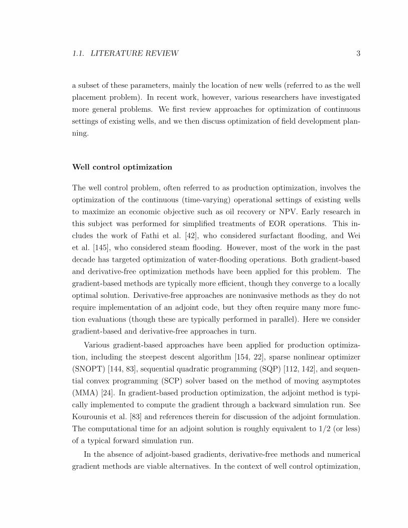
1.1. LITERATURE REVIEW 3
a subset of these parameters, mainly the location of new wells (referred to as the well
placement problem). In recent work, however, various researchers have investigated
more general problems. We first review approaches for optimization of continuous
settings of existing wells, and we then discuss optimization of field development plan-
ning.
Well control optimization
The well control problem, often referred to as production optimization, involves the
optimization of the continuous (time-varying) operational settings of existing wells
to maximize an economic objective such as oil recovery or NPV. Early research in
this subject was performed for simplified treatments of EOR operations. This in-
cludes the work of Fathi et al. [42], who considered surfactant flooding, and Wei
et al. [145], who considered steam flooding. However, most of the work in the past
decade has targeted optimization of water-flooding operations. Both gradient-based
and derivative-free optimization methods have been applied for this problem. The
gradient-based methods are typically more efficient, though they converge to a locally
optimal solution. Derivative-free approaches are noninvasive methods as they do not
require implementation of an adjoint code, but they often require many more func-
tion evaluations (though these are typically performed in parallel). Here we consider
gradient-based and derivative-free approaches in turn.
Various gradient-based approaches have been applied for production optimiza-
tion, including the steepest descent algorithm [154, 22], sparse nonlinear optimizer
(SNOPT) [144, 83], sequential quadratic programming (SQP) [112, 142], and sequen-
tial convex programming (SCP) solver based on the method of moving asymptotes
(MMA) [24]. In gradient-based production optimization, the adjoint method is typi-
cally implemented to compute the gradient through a backward simulation run. See
Kourounis et al. [83] and references therein for discussion of the adjoint formulation.
The computational time for an adjoint solution is roughly equivalent to 1/2 (or less)
of a typical forward simulation run.
In the absence of adjoint-based gradients, derivative-free methods and numerical
gradient methods are viable alternatives. In the context of well control optimization,
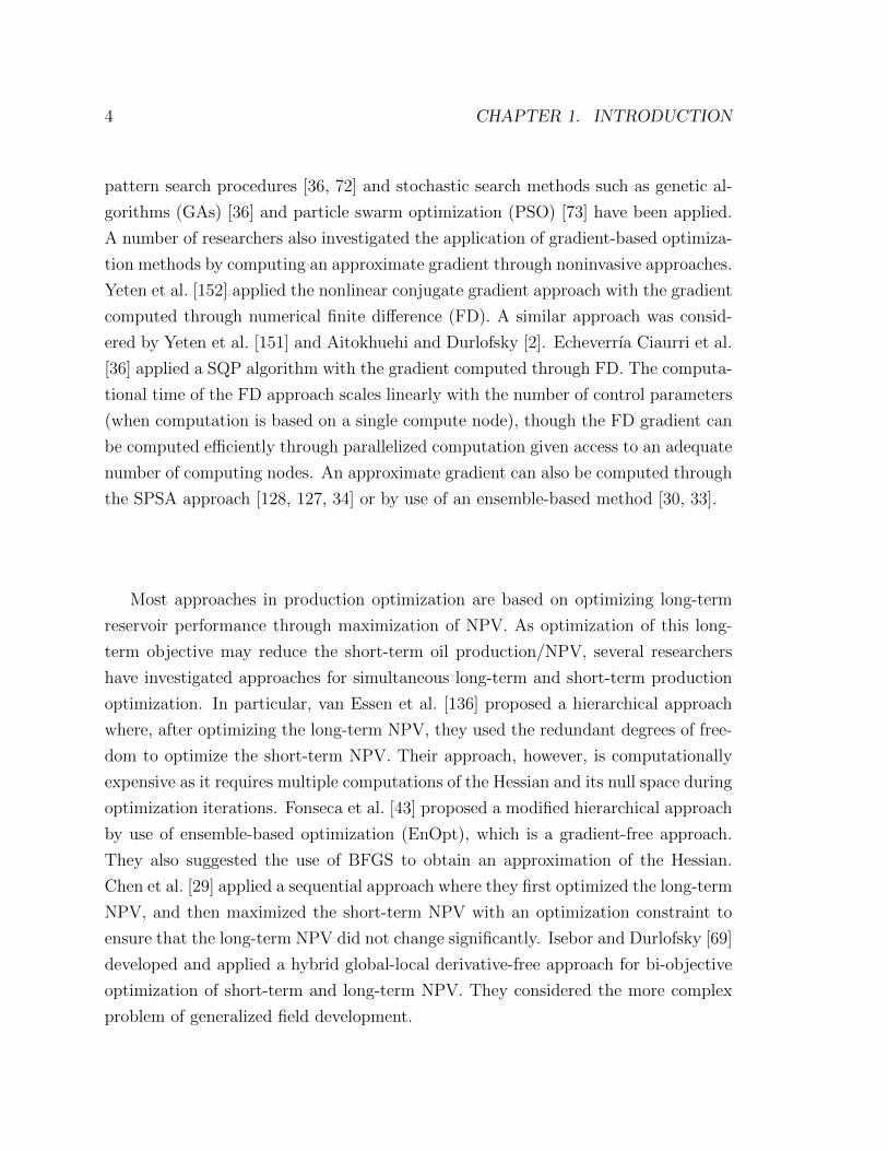
4 CHAPTER 1. INTRODUCTION
pattern search procedures [36, 72] and stochastic search methods such as genetic al-
gorithms (GAs) [36] and particle swarm optimization (PSO) [73] have been applied.
A number of researchers also investigated the application of gradient-based optimiza-
tion methods by computing an approximate gradient through noninvasive approaches.
Yeten et al. [152] applied the nonlinear conjugate gradient approach with the gradient
computed through numerical finite difference (FD). A similar approach was consid-
ered by Yeten et al. [151] and Aitokhuehi and Durlofsky [2]. Echeverrıa Ciaurri et al.
[36] applied a SQP algorithm with the gradient computed through FD. The computa-
tional time of the FD approach scales linearly with the number of control parameters
(when computation is based on a single compute node), though the FD gradient can
be computed efficiently through parallelized computation given access to an adequate
number of computing nodes. An approximate gradient can also be computed through
the SPSA approach [128, 127, 34] or by use of an ensemble-based method [30, 33].
Most approaches in production optimization are based on optimizing long-term
reservoir performance through maximization of NPV. As optimization of this long-
term objective may reduce the short-term oil production/NPV, several researchers
have investigated approaches for simultaneous long-term and short-term production
optimization. In particular, van Essen et al. [136] proposed a hierarchical approach
where, after optimizing the long-term NPV, they used the redundant degrees of free-
dom to optimize the short-term NPV. Their approach, however, is computationally
expensive as it requires multiple computations of the Hessian and its null space during
optimization iterations. Fonseca et al. [43] proposed a modified hierarchical approach
by use of ensemble-based optimization (EnOpt), which is a gradient-free approach.
They also suggested the use of BFGS to obtain an approximation of the Hessian.
Chen et al. [29] applied a sequential approach where they first optimized the long-term
NPV, and then maximized the short-term NPV with an optimization constraint to
ensure that the long-term NPV did not change significantly. Isebor and Durlofsky [69]
developed and applied a hybrid global-local derivative-free approach for bi-objective
optimization of short-term and long-term NPV. They considered the more complex
problem of generalized field development.
1.1. LITERATURE REVIEW 5
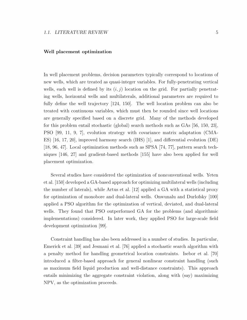
Well placement optimization
In well placement problems, decision parameters typically correspond to locations of
new wells, which are treated as quasi-integer variables. For fully-penetrating vertical
wells, each well is defined by its (i, j) location on the grid. For partially penetrat-
ing wells, horizontal wells and multilaterals, additional parameters are required to
fully define the well trajectory [124, 150]. The well location problem can also be
treated with continuous variables, which must then be rounded since well locations
are generally specified based on a discrete grid. Many of the methods developed
for this problem entail stochastic (global) search methods such as GAs [56, 150, 23],
PSO [99, 11, 9, 7], evolution strategy with covariance matrix adaptation (CMA-
ES) [16, 17, 20], improved harmony search (IHS) [1], and differential evolution (DE)
[18, 96, 47]. Local optimization methods such as SPSA [74, 77], pattern search tech-
niques [146, 27] and gradient-based methods [155] have also been applied for well
placement optimization.
Several studies have considered the optimization of nonconventional wells. Yeten
et al. [150] developed a GA-based approach for optimizing multilateral wells (including
the number of laterals), while Artus et al. [12] applied a GA with a statistical proxy
for optimization of monobore and dual-lateral wells. Onwunalu and Durlofsky [100]
applied a PSO algorithm for the optimization of vertical, deviated, and dual-lateral
wells. They found that PSO outperformed GA for the problems (and algorithmic
implementations) considered. In later work, they applied PSO for large-scale field
development optimization [99].
Constraint handling has also been addressed in a number of studies. In particular,
Emerick et al. [39] and Jesmani et al. [76] applied a stochastic search algorithm with
a penalty method for handling geometrical location constraints. Isebor et al. [70]
introduced a filter-based approach for general nonlinear constraint handling (such
as maximum field liquid production and well-distance constraints). This approach
entails minimizing the aggregate constraint violation, along with (say) maximizing
NPV, as the optimization proceeds.
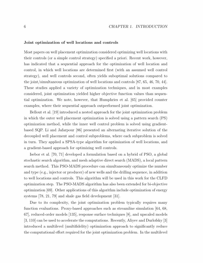
6 CHAPTER 1. INTRODUCTION
Joint optimization of well locations and controls
Most papers on well placement optimization considered optimizing well locations with
their controls (or a simple control strategy) specified a priori. Recent work, however,
has indicated that a sequential approach for the optimization of well location and
control, in which well locations are determined first (with an assumed well control
strategy), and well controls second, often yields suboptimal solutions compared to
the joint/simultaneous optimization of well locations and controls [87, 65, 46, 70, 44].
These studies applied a variety of optimization techniques, and in most examples
considered, joint optimization yielded higher objective function values than sequen-
tial optimization. We note, however, that Humphries et al. [65] provided counter
examples, where their sequential approach outperformed joint optimization.
Bellout et al. [19] introduced a nested approach for the joint optimization problem
in which the outer well placement optimization is solved using a pattern search (PS)
optimization method, while the inner well control problem is solved using gradient-
based SQP. Li and Jafarpour [86] presented an alternating iterative solution of the
decoupled well placement and control subproblems, where each subproblem is solved
in turn. They applied a SPSA-type algorithm for optimization of well locations, and
a gradient-based approach for optimizing well controls.
Isebor et al. [70, 71] developed a formulation based on a hybrid of PSO, a global
stochastic search algorithm, and mesh adaptive direct search (MADS), a local pattern
search method. This PSO-MADS procedure can simultaneously optimize the number
and type (e.g., injector or producer) of new wells and the drilling sequence, in addition
to well locations and controls. This algorithm will be used in this work for the CLFD
optimization step. The PSO-MADS algorithm has also been extended for bi-objective
optimization [69]. Other applications of this algorithm include optimization of energy
systems [78, 21, 79] and shale gas field development [31].
Due to its complexity, the joint optimization problem typically requires many
function evaluations. Proxy-based approaches such as streamline simulation [64, 68,
67], reduced-order models [135], response surface techniques [8], and upscaled models
[3, 110] can be used to accelerate the computations. Recently, Aliyev and Durlofsky [3]
introduced a multilevel (multifidelity) optimization approach to significantly reduce
the computational effort required for the joint optimization problem. In the multilevel
1.1. LITERATURE REVIEW 7
approach [3, 5], the optimization is performed over a sequence of upscaled models of
increasing fidelity. After convergence of the optimizer at a given level, the optimal
solution is used as the initial guess for the next (finer) level. The multilevel approach
has been extended to optimization under geological uncertainty [4].
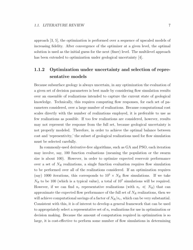
1.1.2 Optimization under uncertainty and selection of repre-
sentative models
Because subsurface geology is always uncertain, in any optimization the evaluation of
a given set of decision parameters is best made by considering flow simulation results
over an ensemble of realizations intended to capture the current state of geological
knowledge. Technically, this requires computing flow responses, for each set of pa-
rameters considered, over a large number of realizations. Because computational cost
scales directly with the number of realizations employed, it is preferable to use as
few realizations as possible. If too few realizations are considered, however, results
may not represent the response from the full set, because geological uncertainty is
not properly modeled. Therefore, in order to achieve the optimal balance between
cost and ‘representivity,’ the subset of geological realizations used for flow simulation
must be selected carefully.
In commonly-used derivative-free algorithms, such as GA and PSO, each iteration
may involve, say, 100 function evaluations (meaning the population or the swarm
size is about 100). However, in order to optimize expected reservoir performance
over a set of NR realizations, a single function evaluation requires flow simulation
to be performed over all of the realizations considered. If an optimization requires
(say) 1000 iterations, this corresponds to 105 × NR flow simulations. If we take
NR to be 100 (which is a typical value), a total of 107 simulations will be required.
However, if we can find nr representative realizations (with nr � NR) that can
approximate the expected flow performance of the full set of NR realizations, then we
will achieve computational savings of a factor of NR/nr, which can be very substantial.
Consistent with this, it is of interest to develop a general framework that can be used
to appropriately select a representative set of nr realizations for use in optimization or
decision making. Because the amount of computation required in optimization is so
large, it is cost-effective to perform some number of flow simulations in determining
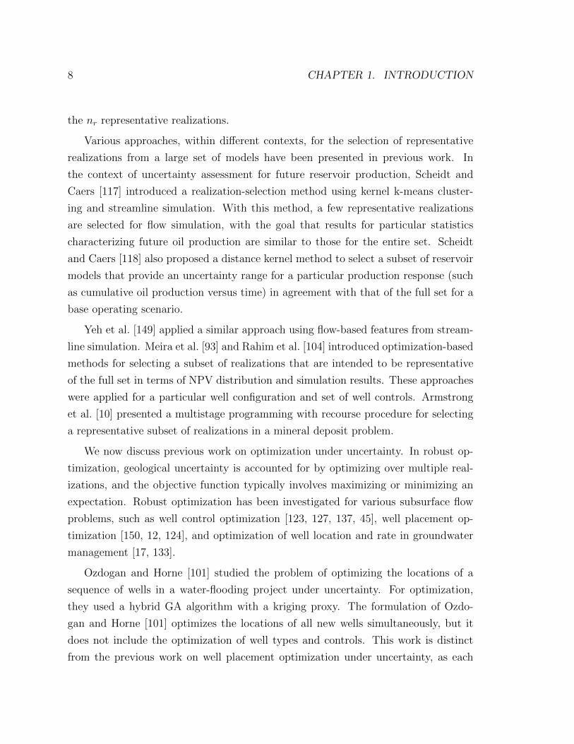
8 CHAPTER 1. INTRODUCTION
the nr representative realizations.
Various approaches, within different contexts, for the selection of representative
realizations from a large set of models have been presented in previous work. In
the context of uncertainty assessment for future reservoir production, Scheidt and
Caers [117] introduced a realization-selection method using kernel k-means cluster-
ing and streamline simulation. With this method, a few representative realizations
are selected for flow simulation, with the goal that results for particular statistics
characterizing future oil production are similar to those for the entire set. Scheidt
and Caers [118] also proposed a distance kernel method to select a subset of reservoir
models that provide an uncertainty range for a particular production response (such
as cumulative oil production versus time) in agreement with that of the full set for a
base operating scenario.
Yeh et al. [149] applied a similar approach using flow-based features from stream-
line simulation. Meira et al. [93] and Rahim et al. [104] introduced optimization-based
methods for selecting a subset of realizations that are intended to be representative
of the full set in terms of NPV distribution and simulation results. These approaches
were applied for a particular well configuration and set of well controls. Armstrong
et al. [10] presented a multistage programming with recourse procedure for selecting
a representative subset of realizations in a mineral deposit problem.
We now discuss previous work on optimization under uncertainty. In robust op-
timization, geological uncertainty is accounted for by optimizing over multiple real-
izations, and the objective function typically involves maximizing or minimizing an
expectation. Robust optimization has been investigated for various subsurface flow
problems, such as well control optimization [123, 127, 137, 45], well placement op-
timization [150, 12, 124], and optimization of well location and rate in groundwater
management [17, 133].
Ozdogan and Horne [101] studied the problem of optimizing the locations of a
sequence of wells in a water-flooding project under uncertainty. For optimization,
they used a hybrid GA algorithm with a kriging proxy. The formulation of Ozdo-
gan and Horne [101] optimizes the locations of all new wells simultaneously, but it
does not include the optimization of well types and controls. This work is distinct
from the previous work on well placement optimization under uncertainty, as each

1.1. LITERATURE REVIEW 9
function evaluation in their optimization involves a history matching step. Further,
they introduced the concept of pseudo-history, which is the ‘probable’ production his-
tory of the next well to be drilled. They defined the pseudo-history to be the future
production data for the realization corresponding to the P50 of the final NPV. Each
function evaluation involves history matching the pseudo-history for all realizations.
In their optimization, they maximized the utility, which is a function of both the
expected NPV and a risk term. They showed that maximizing the utility by inte-
grating pseudo-history in the optimization reduced the risk in terms of the standard
deviation of the final NPV.
Various strategies have been applied to select a representative subset of realizations
for use in optimization. For well control optimization, Shirangi and Mukerji [127]
selected representative realizations by applying k-medoids clustering using some flow-
based features, while Yasari et al. [148] selected realizations based on the ranking of
NPVs obtained from an initial control strategy. For well placement optimization,
Wang et al. [143] applied k-means clustering, using a few static and simulation-based
quantities. Torrado et al. [134] applied a similar approach using only static features.
Yang et al. [147] selected realizations for the robust optimization of well locations in
SAGD operations by ranking models in terms of NPV for a base well location and
control strategy, and then selecting nine realizations corresponding to P10, P20, . . . ,
P90 of the NPV distribution (here P10, P20 and P90 denote the 10th, 20th and 90th
percentiles). Bayer et al. [17, 18] developed a stack ordering approach for identifying
critical realizations for optimization of well locations in groundwater management
problems.
Most of the studies noted above used a single set of realizations throughout the
optimization. These realizations were selected according to their flow response for
a problem involving a particular (base-case) well configuration and control strategy.
Wang et al. [143], however, modified the set of representative realizations during the
course of the optimization based (in part) on the evolving flow response. Previous
studies did not provide procedures to assess whether the selected realizations ade-
quately represented the entire set during the course of the optimization. In addition,
10 CHAPTER 1. INTRODUCTION
there does not appear to have been much study of the impact of the realization-
selection procedure on optimization results. These issues will be addressed in this the-
sis.
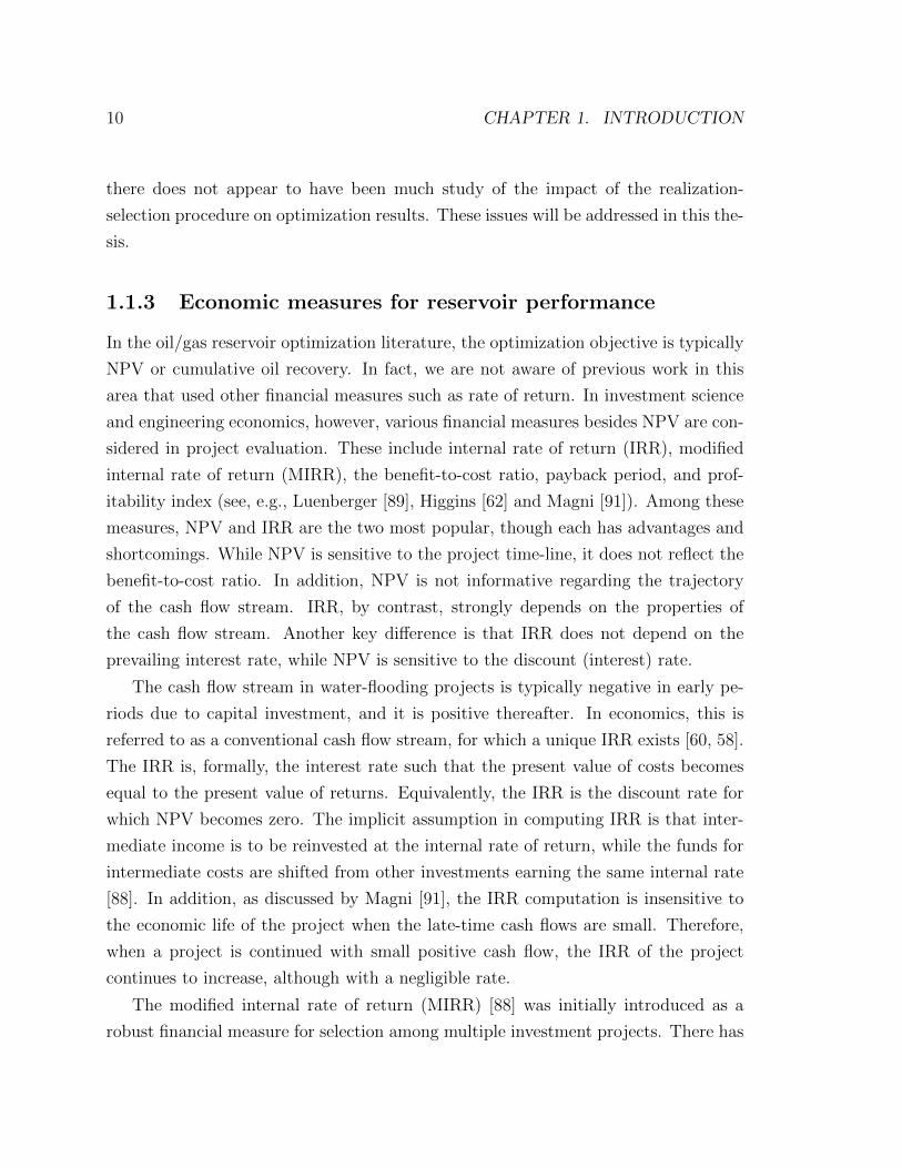
1.1.3 Economic measures for reservoir performance
In the oil/gas reservoir optimization literature, the optimization objective is typically
NPV or cumulative oil recovery. In fact, we are not aware of previous work in this
area that used other financial measures such as rate of return. In investment science
and engineering economics, however, various financial measures besides NPV are con-
sidered in project evaluation. These include internal rate of return (IRR), modified
internal rate of return (MIRR), the benefit-to-cost ratio, payback period, and prof-
itability index (see, e.g., Luenberger [89], Higgins [62] and Magni [91]). Among these
measures, NPV and IRR are the two most popular, though each has advantages and
shortcomings. While NPV is sensitive to the project time-line, it does not reflect the
benefit-to-cost ratio. In addition, NPV is not informative regarding the trajectory
of the cash flow stream. IRR, by contrast, strongly depends on the properties of
the cash flow stream. Another key difference is that IRR does not depend on the
prevailing interest rate, while NPV is sensitive to the discount (interest) rate.
The cash flow stream in water-flooding projects is typically negative in early pe-
riods due to capital investment, and it is positive thereafter. In economics, this is
referred to as a conventional cash flow stream, for which a unique IRR exists [60, 58].
The IRR is, formally, the interest rate such that the present value of costs becomes
equal to the present value of returns. Equivalently, the IRR is the discount rate for
which NPV becomes zero. The implicit assumption in computing IRR is that inter-
mediate income is to be reinvested at the internal rate of return, while the funds for
intermediate costs are shifted from other investments earning the same internal rate
[88]. In addition, as discussed by Magni [91], the IRR computation is insensitive to
the economic life of the project when the late-time cash flows are small. Therefore,
when a project is continued with small positive cash flow, the IRR of the project
continues to increase, although with a negligible rate.
The modified internal rate of return (MIRR) [88] was initially introduced as a
robust financial measure for selection among multiple investment projects. There has
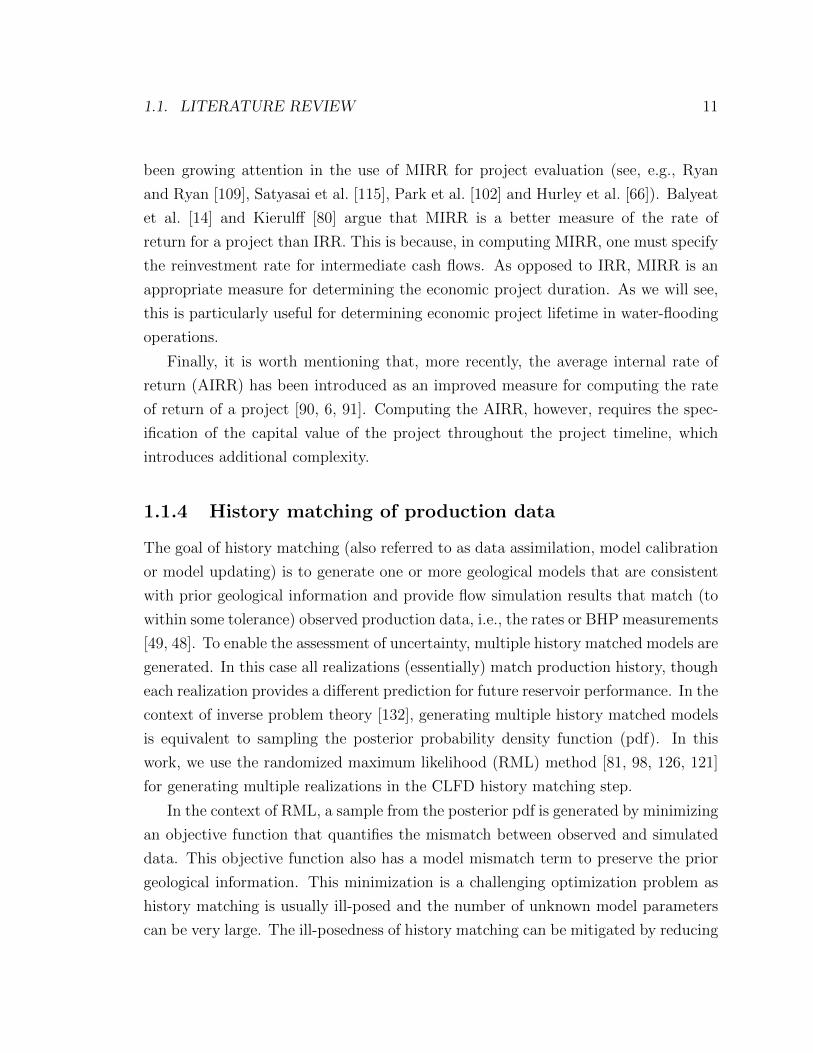
1.1. LITERATURE REVIEW 11
been growing attention in the use of MIRR for project evaluation (see, e.g., Ryan
and Ryan [109], Satyasai et al. [115], Park et al. [102] and Hurley et al. [66]). Balyeat
et al. [14] and Kierulff [80] argue that MIRR is a better measure of the rate of
return for a project than IRR. This is because, in computing MIRR, one must specify
the reinvestment rate for intermediate cash flows. As opposed to IRR, MIRR is an
appropriate measure for determining the economic project duration. As we will see,
this is particularly useful for determining economic project lifetime in water-flooding
operations.
Finally, it is worth mentioning that, more recently, the average internal rate of
return (AIRR) has been introduced as an improved measure for computing the rate
of return of a project [90, 6, 91]. Computing the AIRR, however, requires the spec-
ification of the capital value of the project throughout the project timeline, which
introduces additional complexity.
1.1.4 History matching of production data
The goal of history matching (also referred to as data assimilation, model calibration
or model updating) is to generate one or more geological models that are consistent
with prior geological information and provide flow simulation results that match (to
within some tolerance) observed production data, i.e., the rates or BHP measurements
[49, 48]. To enable the assessment of uncertainty, multiple history matched models are
generated. In this case all realizations (essentially) match production history, though
each realization provides a different prediction for future reservoir performance. In the
context of inverse problem theory [132], generating multiple history matched models
is equivalent to sampling the posterior probability density function (pdf). In this
work, we use the randomized maximum likelihood (RML) method [81, 98, 126, 121]
for generating multiple realizations in the CLFD history matching step.
In the context of RML, a sample from the posterior pdf is generated by minimizing
an objective function that quantifies the mismatch between observed and simulated
data. This objective function also has a model mismatch term to preserve the prior
geological information. This minimization is a challenging optimization problem as
history matching is usually ill-posed and the number of unknown model parameters
can be very large. The ill-posedness of history matching can be mitigated by reducing
12 CHAPTER 1. INTRODUCTION
the number of parameters through an appropriate parameterization such as TSVD
[122, 126], PCA [114, 139], and kernel PCA [114, 141]. Vo and Durlofsky [140, 139]
presented a differentiable PCA-based parameterization that enables application of
efficient gradient-based approaches for history matching complex channelized models.
This optimization-based principal component analysis (O-PCA) approach is used in
the computational results presented in Appendix A of this thesis.
Various optimization methods have been applied for solving the minimization
problem in history matching, including gradient-based methods such as BFGS [124,
51, 50], Gauss-Newton [126], Levenberg-Marquardt algorithm [126, 122, 120], and
SNOPT [139, 140]. Shirangi [122] presented efficient and scalable procedures for
generating multiple realizations of permeability and porosity fields of large-scale three-
dimensional reservoir models. He also introduced the ensemble-based regularization
approach for the efficient computation of the model mismatch term and its derivative
in history matching. Shirangi and Emerick [126] introduced an efficient TSVD-based
Levenberg-Marquardt algorithm for history matching and showed this algorithm to be
more reliable than the Gauss-Newton approach for solving nonlinear inverse problems.
History matching can also be accomplished by use of a Kalman filter [52, 85, 82],
sparsity-based approaches [41, 54], or by ensemble-based data assimilation methods
[30, 97], which do not require the computation of gradients. Joint history matching of
production and seismic data (when available) can result in more uncertainty reduction
than can be achieved using only production data. Recent procedures that use 4D
seismic and production data include those presented by Suman et al. [129], Lee [84],
Echeverrıa Ciaurri et al. [37] and Bukshtynov et al. [24].
1.1.5 Closed-loop reservoir management
The optimal continuous operation of existing wells, often referred to as closed-loop
reservoir management (CLRM), has been the subject of significant research in recent
years [95, 113, 75]. CLRM, depicted in Fig. 1.1, entails optimizing well settings based
on current geological knowledge, operating the reservoir and collecting data over some
time period, and performing data assimilation (history matching) to update the geo-
logical description for consistency with observed data. This procedure, repeated over
the reservoir life, can provide improved performance relative to heuristic approaches
1.1. LITERATURE REVIEW 13
Update Models
CollectReservoir Data
OptimizeWell Settings
Set Well Controls & Operate
Figure 1.1: Schematic of closed-loop reservoir management.
for reservoir management.
Most papers on CLRM investigated the application of particular history match-
ing and optimization approaches for water-flooding operations. Jansen et al. [75]
applied an adjoint-based steepest descent algorithm for production optimization and
the ensemble Kalman filter for data assimilation. They investigated the impact of
optimization frequency on NPV improvement. Aitokhuehi and Durlofsky [2] applied
a nonlinear conjugate gradient approach for optimization and a probability perturba-
tion approach [25] for history matching. They investigated the effect of the number of
history-matched realizations used in optimization on final true-model NPV. A greater
NPV was obtained when multiple realizations were used in optimization than when a
single realization was used. Sarma et al. [112] applied PCA parameterization for his-
tory matching and used the SQP approach for production optimization. Chen et al.
[30] introduced an ensemble-based CLRM implementation in which ensemble-based
methods were applied for both history matching and production optimization.
Bukshtynov et al. [24] introduced a comprehensive adjoint-gradient-based frame-
work for CLRM where automatic differentiation was used in constructing the ad-
joint formulation. They investigated the use of SCP-MMA optimization in CLRM
and showed that this approach outperformed SNOPT for production optimization,
though SNOPT was still preferred for history matching. CLRM has also been applied

14 CHAPTER 1. INTRODUCTION
Update Models
Drill New Well
CollectReservoir Data
Optimize Field Development
Figure 1.2: Schematic of closed-loop field development (CLFD).
to SAGD operations [106, 119], and for the management of geological carbon storage
operations [26].
1.2 Scope of Work
As discussed in Section 1.1.5, closed-loop reservoir management has been investigated
extensively. The treatments used in CLRM, however, are not typically applied for
field development decisions. If computational optimization is even used for field
development, key decisions, such as the optimal number of wells, well types and
locations, are often determined a priori, by optimizing the expected objective (e.g.,
net present value, cumulative oil recovery) over a set of prior geological realizations.
In this work, we develop and apply a general methodology for optimal closed-loop
field development under uncertainty. This new CLFD framework, depicted in Fig. 1.2,
includes (1) solving an optimization problem for the well number, type, location and
controls based on current geological knowledge, (2) sequentially drilling new wells and
collecting data, and (3) performing history matching based on all currently available
data. This process is repeated until the optimal number of wells has been drilled. It
is important to emphasize that the full development plan is (re-)optimized at each
CLFD step; i.e., the location of the next well is determined based on the fact that it
1.2. SCOPE OF WORK 15
is one in a sequence of wells.
Various treatments are also considered for the history matching step in CLFD.
Specifically, procedures are presented for treating both two-point geostatistical (Gaus-
sian) models and channelized reservoir models described by multipoint geostatistics
(MPS). For each case, methods for the integration of hard data and production data
are described.
To accomplish field development optimization over a potentially large number of
geological realizations, we develop a new treatment, which we refer to as optimization
with sample validation (OSV). This approach shares some similarities with the retro-
spective optimization (RO) procedure introduced by Wang et al. [143] for optimizing
over multiple realizations. In RO, instead of optimizing the expected value of the
objective over the entire set of realizations, a sequence of optimization subproblems,
which contain increasing numbers of realizations, is solved. In OSV, the optimization
at each CLFD step is performed over a subset of realizations that are selected to be
representative. Following this optimization, a sample validation procedure is applied
to assess whether these realizations are indeed sufficiently representative of the entire
set. If the subset is found not to be representative, a larger number of realizations is
selected and the optimization step is repeated.
The CLFD framework is very general and various procedures for history matching,
optimization, model selection and economic evaluation can be applied. Following our
development and evaluation of the general CLFD methodology, we focus on two key
components within the overall framework. Specifically, we investigate in detail the
selection of representative models and the application of new economic measures for
reservoir operations. Our intent is to study these two topics as standalone subjects,
as opposed to applying them within the CLFD framework. Integration of these new
treatments into CLFD could be topics for future work.
The OSV procedure developed in the context of CLFD requires an approach to
select a representative subset of models from a large set. While various approaches
have been presented for this, as described earlier, we are not aware of any previous
studies that assessed the performance of different selection methods. In addition, it
is important to recognize that the appropriate selection method may be different in
different contexts. For example, a selected subset that is the most representative for
16 CHAPTER 1. INTRODUCTION
a well control optimization problem (with fixed well locations) may not be the best
choice for a well placement optimization problem, as these two problems are sensitive
to different geological details.
To address these issues, we devise a procedure to quantitatively assess different
selection approaches. We introduce a general clustering method for this purpose.
In this clustering, each realization is represented by a feature vector composed of a
weighted combination of flow-based and geological quantities. Principal component
analysis (PCA) is used to express the geology (permeability field) in terms of a small
number of features, while flow-based features are obtained by solving one or more
base-case flow problems. The use of both full-physics simulations and efficient tracer-
type simulations for obtaining these flow-based features will be considered. We also
investigate the performance of different feature weightings in optimization problems.
In previous work on the optimization of reservoir operations, the project life is
(almost always) specified a priori. The economic project life (EPL) for operation of
existing wells, however, depends on the specific problem and the way in which the
reservoir is operated. Therefore, the project life should be treated as a variable, and
the EPL and well controls should be determined through a joint optimization (that
includes an appropriate definition of rate of return). In this work, we introduce a
nested formulation for the joint optimization of EPL and well controls. In particular,
we show that the use of the modified internal rate of return (MIRR) and the minimum
attractive rate of return (MARR) enables us to jointly determine optimal EPL and
well controls. Our treatments are quite useful in avoiding situations where the NPV
continues to increase in time, but the cash flow is negligible compared to the capital
value of the project.
Consistent with the discussion above, the key research objectives of this work are
as follows:
• Develop a general framework for optimal closed-loop field development op-
timization under uncertainty. Efficient approaches for the optimization and
history matching steps will be implemented. CLFD will be applied to both
Gaussian and channelized reservoir models, which entail different treatments
for history matching.
• Introduce an approach for efficient optimization with model uncertainty (which
1.3. DISSERTATION OUTLINE 17
involves the use of multiple realizations). Toward this goal, optimization with
sample validation is developed and incorporated into the CLFD optimization
step.
• Devise a general methodology for selecting representative models from a large
set of realizations for decision making and optimization under uncertainty. This
includes the introduction of a statistical procedure for comparing various ap-
proaches for this selection.
• Develop a technique to jointly determine the optimal economic project life and
optimal well controls within the context of production optimization.
1.3 Dissertation Outline
In Chapter 2, we describe the CLFD methodology and present extensive numerical re-
sults using this framework. We first introduce the CLFD workflow, and then describe
the optimization and history matching steps. Next, the optimization with sample val-
idation approach is discussed. Computational results are then presented for two- and
three-dimensional Gaussian reservoir models. CLFD results for channelized models
are presented in Appendix A.
In Chapter 3, we investigate the problem of selecting a representative subset of
realizations from a large set. We first define a flow-response vector to assess the qual-
ity of different realization selection approaches. We then present a general method,
based on unsupervised learning techniques, for selecting a representative subset. Var-
ious selection procedures are then assessed for a range of problems, including cases
involving new well locations, new well controls, and production optimization. Differ-
ent algorithmic treatments are considered, as is the use of tracer-type simulations in
place of full-physics simulations. Additional results for binary channelized reservoir
models are presented in Appendix B.
In Chapter 4, we develop and apply a new approach, based on the computation
of modified internal rate of return, for the joint optimization of well controls and
economic project life. We first discuss the computation of modified internal rate of

18 CHAPTER 1. INTRODUCTION
return for water-flooding problems, and then present our procedure for the joint op-
timization. Examples are presented for two- and three-dimensional reservoir models.
Chapter 5 includes a summary, conclusions, and recommendations for future work
in closed-loop field development and related areas.
The new CLFD framework, along with the optimization with sample validation
treatment (described in Chapter 2), has already appeared in an SPE Journal arti-
cle [124]. Our general method for selecting representative realizations, described in
Chapter 3, has been published in Computers & Geosciences [123]. Our new method-
ology for optimizing EPL, described in Chapter 4, has been presented at the 2017
SPE Reservoir Simulation Conference [125].
Chapter 2
Closed-Loop Field Development
Optimization Under Uncertainty
In this chapter, we first describe the closed-loop field development (CLFD) optimiza-
tion framework, including the procedures used for optimization and history matching.
The selection of representative realizations to use for optimization, and optimization
with sample validation, are then discussed. We next present computational results for
two- and three-dimensional examples that demonstrate the application and potential
benefits of CLFD. We end this chapter with a brief summary.
2.1 CLFD workflow
We consider the field development optimization problem in which decisions such as
the number, types, drilling sequence, locations and time-varying controls of new wells
are to be determined. The term ‘decision variables’ is used to refer to the associated
optimization variables. The reservoir is initially described by a set of prior geological
realizations. New wells are to be drilled sequentially, one (or a few) at a time, as is
commonly the case in practice.
The CLFD optimization workflow entails solving an optimization problem to de-
termine the decision variables for new and existing wells (future well control variables
are determined for existing wells), ‘drilling’ a new well and collecting the associated
data, and performing history matching based on all available data. At each step of
19
20 CHAPTER 2. CLOSED-LOOP FIELD DEVELOPMENT
the procedure, the overall future development/operating plan is optimized; i.e., the
location for the next well is determined with the knowledge that it is one well within
a sequence of wells. Optimization is performed over multiple realizations to account
for uncertainty. While we use a particular set of methods in the optimization and
history matching steps of CLFD, the framework is general and different methods can
be employed.
Similar to closed-loop reservoir management (CLRM), the CLFD workflow in-
cludes optimization and history matching steps. The optimization step in CLFD is,
however, much more complex as it involves categorical (number/type and drilling
schedule for new wells), quasi-integer (well location), and continuous (well control)
variables. This is in contrast to CLRM, which entails only well control variables. The
CLFD history matching step is also slightly different from that in CLRM. This is be-
cause, in CLFD, the observed data include both production data and hard data (e.g.,
measured values of porosity or permeability) at well locations. In CLRM, hard data
are known a priori and are thus treated differently in the history matching procedure.
In all of our computational experiments, ‘observed’ production data are generated by
simulating a model selected randomly from the prior distribution. This model, which
also provides hard data at well locations, is referred to as the ‘true model.’
We now describe the CLFD framework for the case where one well is drilled at
a time. Extension to more general cases in which two or more wells are drilled at
a time is straightforward. Let t1, t2, . . . ti, . . . tn denote a discrete time series, where
ti indicates the time (in days) that production/injection for Well i is started. We
assume that the location and type (injector or producer) of Well i are determined at
time ti−1, and that Well i is drilled during the period (ti−1, ti), which corresponds to
control step i − 1. It is also possible that, depending on the problem definition, the
optimal solution may be not to drill Well i.
Our approach for CLFD is illustrated in Fig. 2.1. The notation used in the figure
and throughout this chapter is as follows. The vector x defines the decision variables
for all wells. The maximum number of wells is denoted by nw. There can be fewer
than nw wells since in the optimization some wells may be determined to be of type ‘do
not drill’ (rather than injector or producer). A current (time ti) geological realization
is denoted by mij, with j = 1, . . . , NR, where NR is the number of realizations. For
2.1. CLFD WORKFLOW 21
the case where the geological model is fully described by a single value in each grid
block, mij will be of dimension Nb, where Nb is the number of grid blocks in the model.
Each of the current realizations is inserted (as a column) into the matrix M i, which
is thus of dimensions Nb × NR. The optimization problem entails maximization of
expected net present value (NPV) of the field development project. Expected NPV
is denoted by J .
CLFD proceeds as illustrated in Fig. 2.1. The set of initial (prior) realizations is
designated M1. Using these models, and x0 as the initial guess for the field develop-
ment decision variables (which could be user provided or generated randomly), the
optimization problem is solved to provide x1. The PSO-MADS hybrid algorithm is
used for this optimization. The optimal solution x1 defines the location and type of
Wells 1 and 2. Production from Well 1 starts at t1 (using the optimal setting) and
Well 2 is drilled during the period (t1, t2).
The first CLFD history matching is performed at t2 (Fig. 2.1). In this compu-
tation, we use production data from Well 1 and hard data from Well 1 and (newly
drilled) Well 2 to determine a new set of conditioned realizations M2. The next
optimization is performed using realizations M2, with x1 as the initial guess. This
computation provides the new optimal solution x2. As prescribed by x2, Well 3 is
then drilled, and the controls of Wells 1 and 2 are set for the next control step. This
procedure is repeated until a maximum of nw wells has been drilled. It is important
to emphasize that, at each CLFD step, the full field development plan is updated; i.e.,
the locations, types and controls for all future wells are determined. Thus, when each
new well is drilled, the fact that additional (planned) wells will be drilled is taken
into account. The locations and types of the planned wells are, however, updated in
subsequent CLFD steps.
In the history matching performed at time ti, the current realizations (conditioned
to all data up to time ti−1) are used as the initial guesses. The total history matching
period is from t1 to ti. After performing this history matching step, the simulation
state variables (phase pressures and saturations) are saved to restart files. During
optimization, all reservoir simulations start at time ti and proceed until time T (the
end of the reservoir life). This avoids repeating the simulation for the time period
before ti and thus enhances overall computational efficiency.
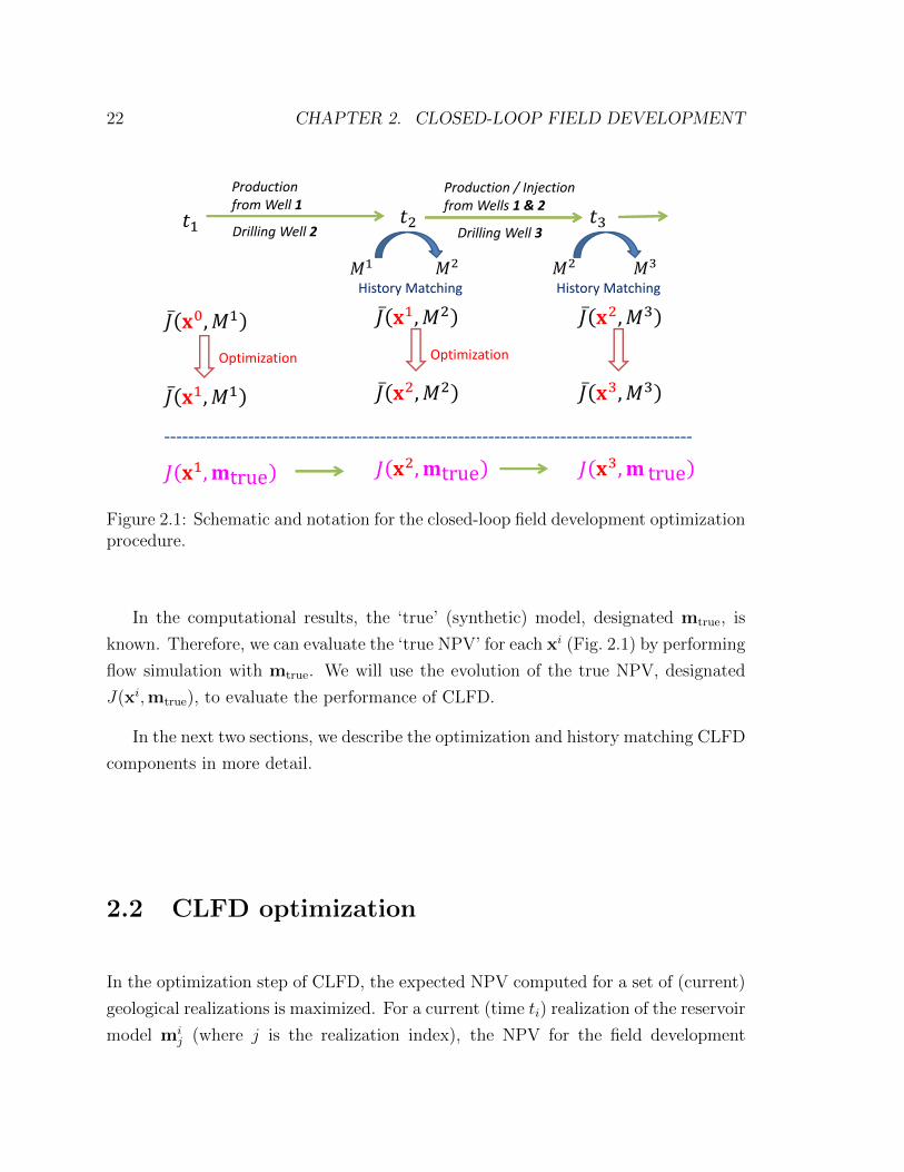
22 CHAPTER 2. CLOSED-LOOP FIELD DEVELOPMENT
History Matching History Matching
Optimization Optimization
Productionfrom Well 1
Production / Injectionfrom Wells 1 & 2
Drilling Well 2 Drilling Well 3
Figure 2.1: Schematic and notation for the closed-loop field development optimizationprocedure.
In the computational results, the ‘true’ (synthetic) model, designated mtrue, is
known. Therefore, we can evaluate the ‘true NPV’ for each xi (Fig. 2.1) by performing
flow simulation with mtrue. We will use the evolution of the true NPV, designated
J(xi,mtrue), to evaluate the performance of CLFD.
In the next two sections, we describe the optimization and history matching CLFD
components in more detail.
2.2 CLFD optimization
In the optimization step of CLFD, the expected NPV computed for a set of (current)
geological realizations is maximized. For a current (time ti) realization of the reservoir
model mij (where j is the realization index), the NPV for the field development
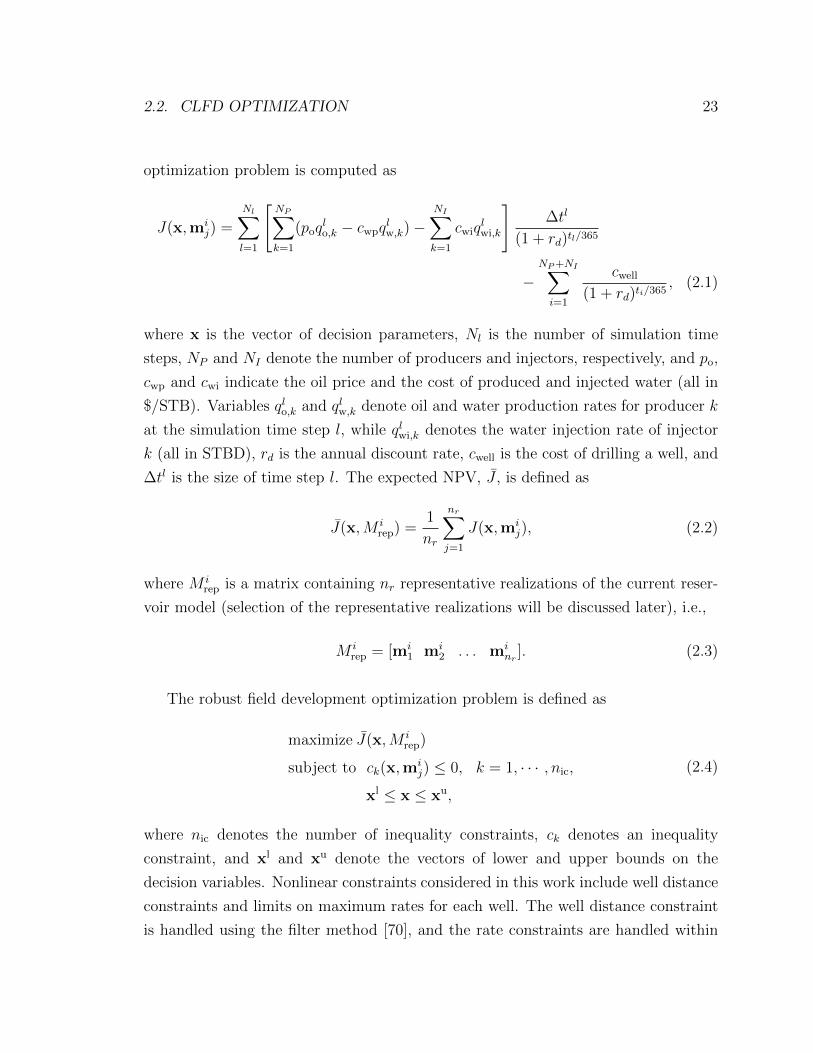
2.2. CLFD OPTIMIZATION 23
optimization problem is computed as
J(x,mij) =
Nl∑l=1
[NP∑k=1
(poqlo,k − cwpq
lw,k)−
NI∑k=1
cwiqlwi,k
]∆tl
(1 + rd)tl/365
−NP+NI∑i=1
cwell(1 + rd)ti/365
, (2.1)
where x is the vector of decision parameters, Nl is the number of simulation time
steps, NP and NI denote the number of producers and injectors, respectively, and po,
cwp and cwi indicate the oil price and the cost of produced and injected water (all in
$/STB). Variables qlo,k and qlw,k denote oil and water production rates for producer k
at the simulation time step l, while qlwi,k denotes the water injection rate of injector
k (all in STBD), rd is the annual discount rate, cwell is the cost of drilling a well, and
∆tl is the size of time step l. The expected NPV, J , is defined as
J(x,M irep) =
1
nr
nr∑j=1
J(x,mij), (2.2)
where M irep is a matrix containing nr representative realizations of the current reser-
voir model (selection of the representative realizations will be discussed later), i.e.,
M irep = [mi
1 mi2 . . . mi
nr]. (2.3)
The robust field development optimization problem is defined as
maximize J(x,M irep)
subject to ck(x,mij) ≤ 0, k = 1, · · · , nic,
xl ≤ x ≤ xu,
(2.4)
where nic denotes the number of inequality constraints, ck denotes an inequality
constraint, and xl and xu denote the vectors of lower and upper bounds on the
decision variables. Nonlinear constraints considered in this work include well distance
constraints and limits on maximum rates for each well. The well distance constraint
is handled using the filter method [70], and the rate constraints are handled within
24 CHAPTER 2. CLOSED-LOOP FIELD DEVELOPMENT
the forward simulation. The optimal solution computed at ti is denoted by xi, and
the corresponding optimal value is J(xi,M irep). The initial guess for optimization
at time ti is the optimal solution at ti−1 (i.e., xi−1). During optimization at ti, all
parameters corresponding to decisions prior to ti are held as constant.
All optimizations in this work are performed using PSO-MADS. See Isebor et al.
[70, 71] for full details on the procedure and for a number of examples that demon-
strate algorithmic performance. For a concise description of the individual PSO and
MADS algorithms, and the PSO-MADS hybrid, see Aliyev and Durlofsky [3]. PSO is a
stochastic population-based cooperative-search algorithm that provides some amount
of global exploration but is not guaranteed to converge to a (local or global) min-
imum. Each PSO ‘particle’ represents a potential solution (e.g., well configuration
and controls), which moves through the search space based on a set of ‘velocity’ com-
ponents. MADS, by contrast, is a pattern search method that provides convergence,
in many cases, to a local minimum. By combining these two procedures, we achieve
global search along with local convergence (it is important to note, however, that the
PSO-MADS algorithm does not in general find the global optimum). Examples in
Isebor et al. [70] highlight the advantages of the PSO-MADS hybrid over standalone
PSO and MADS.
The method requires a large number of function evaluations, each of which entails
nr flow simulations. Because both PSO and MADS parallelize naturally, elapsed
times, which in this work correspond to the time required to perform hundreds to
a few thousand simulations, are not overly excessive assuming simulation run times
are on the order of minutes. PSO-MADS termination criteria can be based on a
minimum improvement in the objective function, a minimum stencil size in MADS, or
a maximum number of function evaluations. At early steps of CLFD, the algorithm
typically terminates when a maximum number of function evaluations is reached,
while at later steps, termination is usually due to one of the other criteria.
2.3. OPTIMIZATION WITH SAMPLE VALIDATION 25
2.3 Optimization with sample validation and de-
termination of representative realizations
The number of simulations that must be performed in CLFD is directly proportional
to the number of realizations considered (as is evident from Eq. 2.2). This means it
is beneficial to use as few realizations as possible. It is also important to note that
the CLFD optimization usually requires many more flow simulations than the history
matching component. Thus, it is relatively inexpensive to generate ‘excess’ history
matched models.
These observations motivate the optimization with sample validation (OSV) pro-
cedure used in this work. We first describe the sample validation method and then the
overall procedure. Assume that a large number (NR) of realizations have been gener-
ated in the most recent history matching step. We wish to perform optimization using
a subset (nr) of ‘representative’ realizations. We will discuss later how representative
realizations are selected. With Mrep denoting a set of nr representative realizations
and xi−1 indicating the initial guess for the current optimization, the PSO-MADS
algorithm provides an optimum set of decision variables xi by optimizing over the
Mrep realizations. The increase in J achieved in this optimization step is given by
J(xi,Mrep)− J(xi−1,Mrep).
Our interest, however, is in maximizing the expected NPV over the entire cur-
rent set of NR realizations, denoted by M . We assess this quantity by computing
J(xi,M) − J(xi−1,M) after the optimization over Mrep has been completed. The
validation procedure requires that the ratio of the increase in J for NR realizations
relative to the increase in J for nr realizations exceeds a threshold parameter θ. We
call this ratio the relative improvement RI and express the validation criterion as:
RI =J(xi,M)− J(xi−1,M)
J(xi,Mrep)− J(xi−1,Mrep)≥ θ. (2.5)
In this work we use θ = 0.5, though of course other values could be used if we wish
to be more or less stringent. If Eq. 2.5 is not satisfied, we choose a larger number
of representative realizations (by increasing nr) and repeat the optimization (i.e.,
proceed to the next subproblem) to provide a new xi. This process terminates when
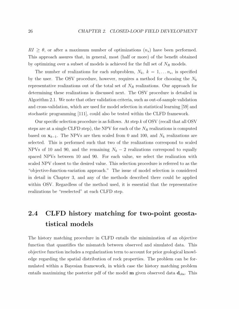
26 CHAPTER 2. CLOSED-LOOP FIELD DEVELOPMENT
RI ≥ θ, or after a maximum number of optimizations (ns) have been performed.
This approach assures that, in general, most (half or more) of the benefit obtained
by optimizing over a subset of models is achieved for the full set of NR models.
The number of realizations for each subproblem, Nk, k = 1, . . . ns, is specified
by the user. The OSV procedure, however, requires a method for choosing the Nk
representative realizations out of the total set of NR realizations. Our approach for
determining these realizations is discussed next. The OSV procedure is detailed in
Algorithm 2.1. We note that other validation criteria, such as out-of-sample validation
and cross-validation, which are used for model selection in statistical learning [59] and
stochastic programming [111], could also be tested within the CLFD framework.
Our specific selection procedure is as follows. At step k of OSV (recall that all OSV
steps are at a single CLFD step), the NPV for each of the NR realizations is computed
based on xk−1. The NPVs are then scaled from 0 and 100, and Nk realizations are
selected. This is performed such that two of the realizations correspond to scaled
NPVs of 10 and 90, and the remaining Nk − 2 realizations correspond to equally
spaced NPVs between 10 and 90. For each value, we select the realization with
scaled NPV closest to the desired value. This selection procedure is referred to as the
“objective-function-variation approach.” The issue of model selection is considered
in detail in Chapter 3, and any of the methods described there could be applied
within OSV. Regardless of the method used, it is essential that the representative
realizations be “reselected” at each CLFD step.
2.4 CLFD history matching for two-point geosta-
tistical models
The history matching procedure in CLFD entails the minimization of an objective
function that quantifies the mismatch between observed and simulated data. This
objective function includes a regularization term to account for prior geological knowl-
edge regarding the spatial distribution of rock properties. The problem can be for-
mulated within a Bayesian framework, in which case the history matching problem
entails maximizing the posterior pdf of the model m given observed data dobs. This

2.4. CLFD HISTORY MATCHING 27
Algorithm 2.1 Optimization with sample validation
Specify initial guess x0 (x0 = xi−1)for k = 1, 2, . . . , ns do
Select a set of Nk representative realizations, Mkrep = [m1 m2 . . . mNk
], usingthe objective-function-variation approachObtain xk as argmaxxJ(x,Mk
rep) using xk−1 as the initial guessEvaluate RI in Eq. 2.5 (by replacing Mrep by Mk
rep and xi by xk)if the sample validation criterion is satisfied (RI ≥ θ), then
set xi = xk and terminate the loopend ifif k = ns then
set xi = argmaxxk,k=1,...ns(J(xk,M))
end ifend for
can be expressed as [132]
f(m|dobs) = a exp(−S(m)), (2.6)
where a is the normalizing constant and S(m), referred to as the total objective
function, is given by
S(m) =1
2(m−mprior)
TC−1m (m−mprior) +
1
2(gp(m)− dpobs)
TC−1d,p(gp(m)− dpobs)
+1
2(gh(m)− dhobs)
TC−1d,h(gh(m)− dhobs)
= Sm(m) + Spd(m) + Shd (m).
(2.7)
Here Sm is the model mismatch term, Spd is the production data mismatch term, Shd is
the hard data mismatch term, mprior is the mean of the prior model, Cm denotes the
prior covariance matrix, dpobs and dhobs, of dimensions Npd and Nh
d indicate the vectors
of observed production data and hard data, gp(m) and gh(m) denote the vectors
of predicted production data and hard data, Cd,p indicates the Npd×N
pd (diagonal)
covariance matrix for the measurement error in production data, and Cd,h is the
Nhd×Nh
d (diagonal) covariance matrix for the measurement error in hard data.
The maximum a posteriori (MAP) estimate is the model that maximizes Eq. 2.6,
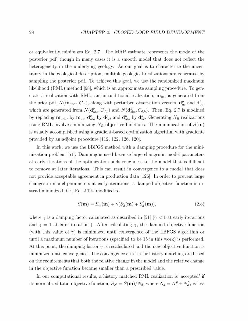
28 CHAPTER 2. CLOSED-LOOP FIELD DEVELOPMENT
or equivalently minimizes Eq. 2.7. The MAP estimate represents the mode of the
posterior pdf, though in many cases it is a smooth model that does not reflect the
heterogeneity in the underlying geology. As our goal is to characterize the uncer-
tainty in the geological description, multiple geological realizations are generated by
sampling the posterior pdf. To achieve this goal, we use the randomized maximum
likelihood (RML) method [98], which is an approximate sampling procedure. To gen-
erate a realization with RML, an unconditional realization, muc, is generated from
the prior pdf, N(mprior, Cm), along with perturbed observation vectors, dpuc and dhuc,
which are generated from N(dpobs, Cd,p) and N(dhobs, Cd,h). Then, Eq. 2.7 is modified
by replacing mprior by muc, dpobs by dpuc, and dhobs by dhuc. Generating NR realizations
using RML involves minimizing NR objective functions. The minimization of S(m)
is usually accomplished using a gradient-based optimization algorithm with gradients
provided by an adjoint procedure [112, 122, 126, 120].
In this work, we use the LBFGS method with a damping procedure for the mini-
mization problem [51]. Damping is used because large changes in model parameters
at early iterations of the optimization adds roughness to the model that is difficult
to remove at later iterations. This can result in convergence to a model that does
not provide acceptable agreement in production data [126]. In order to prevent large
changes in model parameters at early iterations, a damped objective function is in-
stead minimized, i.e., Eq. 2.7 is modified to
S(m) = Sm(m) + γ(Spd(m) + Shd (m)), (2.8)
where γ is a damping factor calculated as described in [51] (γ < 1 at early iterations
and γ = 1 at later iterations). After calculating γ, the damped objective function
(with this value of γ) is minimized until convergence of the LBFGS algorithm or
until a maximum number of iterations (specified to be 15 in this work) is performed.
At this point, the damping factor γ is recalculated and the new objective function is
minimized until convergence. The convergence criteria for history matching are based
on the requirements that both the relative change in the model and the relative change
in the objective function become smaller than a prescribed value.
In our computational results, a history matched RML realization is ‘accepted’ if
its normalized total objective function, SN = S(m)/Nd, where Nd = Npd +Nh
d , is less

2.5. COMPUTATIONAL RESULTS 29
than a specified value (here we require SN ≤ 5). Otherwise, the realization is not
considered to be a sample of the posterior pdf. Relatively few (e.g., < 5%) of the
generated realizations are discarded based on this requirement.
Because the RML runs are independent of one another, each RML realization
can be generated on a separate compute node using distributed computing. We
use Stanford’s Automatic Differentiation-based General Purpose Research Simulator,
AD-GPRS [157] for our computational experiments. The existing OpenMP-based
parallelized version of AD-GPRS [156] allows us to run each simulation on a compu-
tational node with 16 cores. This gives an average speedup of about a factor of 10 for
each simulation. The gradient for history matching is generated using the automatic
differentiation framework [83, 24]. For the CLFD results presented in this work, at
each history matching step, we generate NR = 50 posterior RML realizations plus
the MAP estimate. These models are all generated simultaneously using 51 compute
nodes.
2.5 Computational results
We now apply the CLFD procedure to three example cases, all involving oil-water
systems. In Example 2.1, simultaneous and sequential (well-by-well) optimization of
a field development scenario are compared for a deterministic reservoir description.
In Examples 2 and 3, the CLFD optimization framework is applied to two- and three-
dimensional reservoir models. The effectiveness of the sample validation procedure
is illustrated in these examples. An example involving a channelized reservoir is
presented in Appendix A.
2.5.1 Example 2.1: Simultaneous versus sequential optimiza-
tion of field development
In CLFD optimization, the goal is to determine near-term decision variables in light
of the overall field development plan (i.e., with recognition that the next well is one
well in a sequence). Optimization of immediate decisions without considering future
decisions is essentially a ‘greedy’ approach, which will in general result in a suboptimal
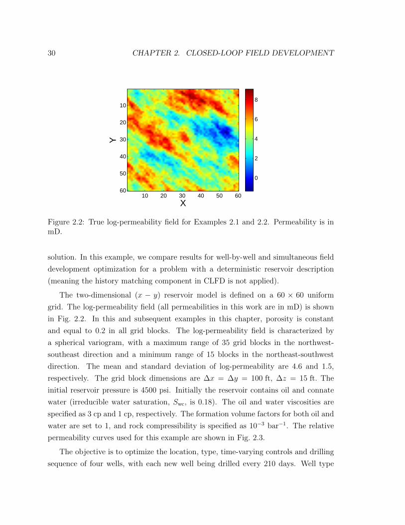
30 CHAPTER 2. CLOSED-LOOP FIELD DEVELOPMENT
X
Y
10 20 30 40 50 60
10
20
30
40
50
60
0
2
4
6
8
Figure 2.2: True log-permeability field for Examples 2.1 and 2.2. Permeability is inmD.
solution. In this example, we compare results for well-by-well and simultaneous field
development optimization for a problem with a deterministic reservoir description
(meaning the history matching component in CLFD is not applied).
The two-dimensional (x − y) reservoir model is defined on a 60 × 60 uniform
grid. The log-permeability field (all permeabilities in this work are in mD) is shown
in Fig. 2.2. In this and subsequent examples in this chapter, porosity is constant
and equal to 0.2 in all grid blocks. The log-permeability field is characterized by
a spherical variogram, with a maximum range of 35 grid blocks in the northwest-
southeast direction and a minimum range of 15 blocks in the northeast-southwest
direction. The mean and standard deviation of log-permeability are 4.6 and 1.5,
respectively. The grid block dimensions are ∆x = ∆y = 100 ft, ∆z = 15 ft. The
initial reservoir pressure is 4500 psi. Initially the reservoir contains oil and connate
water (irreducible water saturation, Swc, is 0.18). The oil and water viscosities are
specified as 3 cp and 1 cp, respectively. The formation volume factors for both oil and
water are set to 1, and rock compressibility is specified as 10−3 bar−1. The relative
permeability curves used for this example are shown in Fig. 2.3.
The objective is to optimize the location, type, time-varying controls and drilling
sequence of four wells, with each new well being drilled every 210 days. Well type
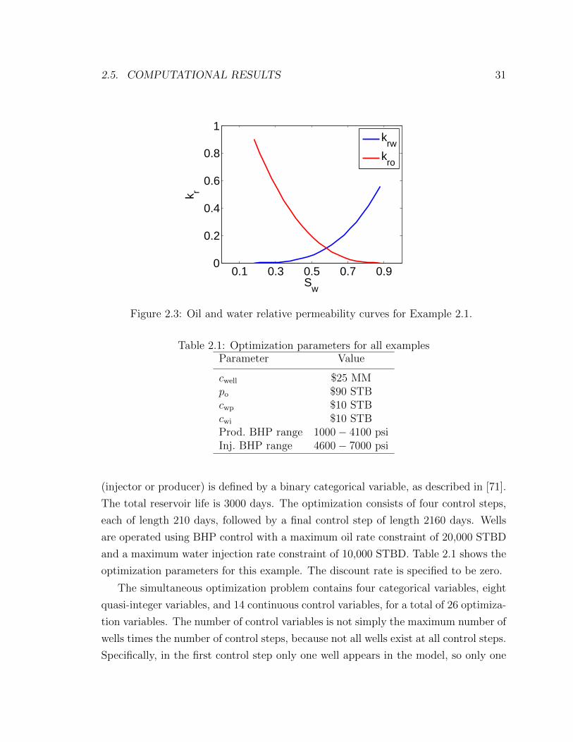
2.5. COMPUTATIONAL RESULTS 31
0.1 0.3 0.5 0.7 0.90
0.2
0.4
0.6
0.8
1
Sw
k r
krw
kro
Figure 2.3: Oil and water relative permeability curves for Example 2.1.
Table 2.1: Optimization parameters for all examplesParameter Value
cwell $25 MMpo $90 STBcwp $10 STBcwi $10 STBProd. BHP range 1000− 4100 psiInj. BHP range 4600− 7000 psi
(injector or producer) is defined by a binary categorical variable, as described in [71].
The total reservoir life is 3000 days. The optimization consists of four control steps,
each of length 210 days, followed by a final control step of length 2160 days. Wells
are operated using BHP control with a maximum oil rate constraint of 20,000 STBD
and a maximum water injection rate constraint of 10,000 STBD. Table 2.1 shows the
optimization parameters for this example. The discount rate is specified to be zero.
The simultaneous optimization problem contains four categorical variables, eight
quasi-integer variables, and 14 continuous control variables, for a total of 26 optimiza-
tion variables. The number of control variables is not simply the maximum number of
wells times the number of control steps, because not all wells exist at all control steps.
Specifically, in the first control step only one well appears in the model, so only one
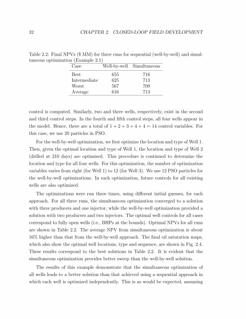
32 CHAPTER 2. CLOSED-LOOP FIELD DEVELOPMENT
Table 2.2: Final NPVs ($ MM) for three runs for sequential (well-by-well) and simul-taneous optimization (Example 2.1)
Case Well-by-well Simultaneous
Best 655 716Intermediate 625 713Worst 567 709Average 616 713
control is computed. Similarly, two and three wells, respectively, exist in the second
and third control steps. In the fourth and fifth control steps, all four wells appear in
the model. Hence, there are a total of 1 + 2 + 3 + 4 + 4 = 14 control variables. For
this case, we use 20 particles in PSO.
For the well-by-well optimization, we first optimize the location and type of Well 1.
Then, given the optimal location and type of Well 1, the location and type of Well 2
(drilled at 210 days) are optimized. This procedure is continued to determine the
location and type for all four wells. For this optimization, the number of optimization
variables varies from eight (for Well 1) to 12 (for Well 3). We use 12 PSO particles for
the well-by-well optimizations. In each optimization, future controls for all existing
wells are also optimized.
The optimizations were run three times, using different initial guesses, for each
approach. For all three runs, the simultaneous optimization converged to a solution
with three producers and one injector, while the well-by-well optimization provided a
solution with two producers and two injectors. The optimal well controls for all cases
correspond to fully open wells (i.e., BHPs at the bounds). Optimal NPVs for all runs
are shown in Table 2.2. The average NPV from simultaneous optimization is about
16% higher than that from the well-by-well approach. The final oil saturation maps,
which also show the optimal well locations, type and sequence, are shown in Fig. 2.4.
These results correspond to the best solutions in Table 2.2. It is evident that the
simultaneous optimization provides better sweep than the well-by-well solution.
The results of this example demonstrate that the simultaneous optimization of
all wells leads to a better solution than that achieved using a sequential approach in
which each well is optimized independently. This is as would be expected, assuming
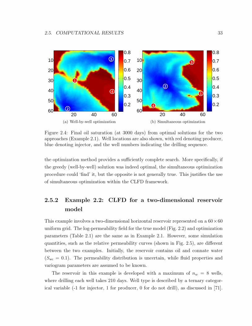
2.5. COMPUTATIONAL RESULTS 33
2
3
1
4
20 40 60
10
20
30
40
50
600.2
0.3
0.4
0.5
0.6
0.7
0.8
(a) Well-by-well optimization
2
1
3
4
20 40 60
10
20
30
40
50
600.2
0.3
0.4
0.5
0.6
0.7
0.8
(b) Simultaneous optimization
Figure 2.4: Final oil saturation (at 3000 days) from optimal solutions for the twoapproaches (Example 2.1). Well locations are also shown, with red denoting producer,blue denoting injector, and the well numbers indicating the drilling sequence.
the optimization method provides a sufficiently complete search. More specifically, if
the greedy (well-by-well) solution was indeed optimal, the simultaneous optimization
procedure could ‘find’ it, but the opposite is not generally true. This justifies the use
of simultaneous optimization within the CLFD framework.
2.5.2 Example 2.2: CLFD for a two-dimensional reservoir
model
This example involves a two-dimensional horizontal reservoir represented on a 60×60
uniform grid. The log-permeability field for the true model (Fig. 2.2) and optimization
parameters (Table 2.1) are the same as in Example 2.1. However, some simulation
quantities, such as the relative permeability curves (shown in Fig. 2.5), are different
between the two examples. Initially, the reservoir contains oil and connate water
(Swc = 0.1). The permeability distribution is uncertain, while fluid properties and
variogram parameters are assumed to be known.
The reservoir in this example is developed with a maximum of nw = 8 wells,
where drilling each well takes 210 days. Well type is described by a ternary categor-
ical variable (-1 for injector, 1 for producer, 0 for do not drill), as discussed in [71].
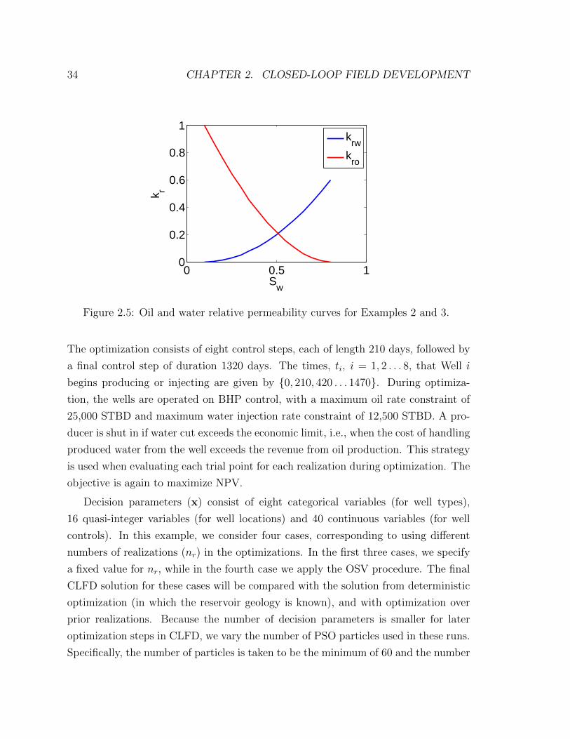
34 CHAPTER 2. CLOSED-LOOP FIELD DEVELOPMENT
0 0.5 10
0.2
0.4
0.6
0.8
1
Sw
k r
krw
kro
Figure 2.5: Oil and water relative permeability curves for Examples 2 and 3.
The optimization consists of eight control steps, each of length 210 days, followed by
a final control step of duration 1320 days. The times, ti, i = 1, 2 . . . 8, that Well i
begins producing or injecting are given by {0, 210, 420 . . . 1470}. During optimiza-
tion, the wells are operated on BHP control, with a maximum oil rate constraint of
25,000 STBD and maximum water injection rate constraint of 12,500 STBD. A pro-
ducer is shut in if water cut exceeds the economic limit, i.e., when the cost of handling
produced water from the well exceeds the revenue from oil production. This strategy
is used when evaluating each trial point for each realization during optimization. The
objective is again to maximize NPV.
Decision parameters (x) consist of eight categorical variables (for well types),
16 quasi-integer variables (for well locations) and 40 continuous variables (for well
controls). In this example, we consider four cases, corresponding to using different
numbers of realizations (nr) in the optimizations. In the first three cases, we specify
a fixed value for nr, while in the fourth case we apply the OSV procedure. The final
CLFD solution for these cases will be compared with the solution from deterministic
optimization (in which the reservoir geology is known), and with optimization over
prior realizations. Because the number of decision parameters is smaller for later
optimization steps in CLFD, we vary the number of PSO particles used in these runs.
Specifically, the number of particles is taken to be the minimum of 60 and the number
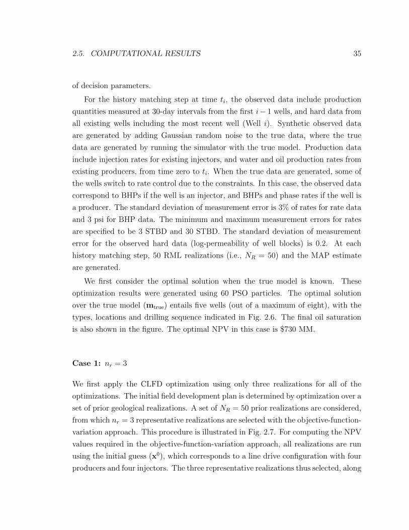
2.5. COMPUTATIONAL RESULTS 35
of decision parameters.
For the history matching step at time ti, the observed data include production
quantities measured at 30-day intervals from the first i− 1 wells, and hard data from
all existing wells including the most recent well (Well i). Synthetic observed data
are generated by adding Gaussian random noise to the true data, where the true
data are generated by running the simulator with the true model. Production data
include injection rates for existing injectors, and water and oil production rates from
existing producers, from time zero to ti. When the true data are generated, some of
the wells switch to rate control due to the constraints. In this case, the observed data
correspond to BHPs if the well is an injector, and BHPs and phase rates if the well is
a producer. The standard deviation of measurement error is 3% of rates for rate data
and 3 psi for BHP data. The minimum and maximum measurement errors for rates
are specified to be 3 STBD and 30 STBD. The standard deviation of measurement
error for the observed hard data (log-permeability of well blocks) is 0.2. At each
history matching step, 50 RML realizations (i.e., NR = 50) and the MAP estimate
are generated.
We first consider the optimal solution when the true model is known. These
optimization results were generated using 60 PSO particles. The optimal solution
over the true model (mtrue) entails five wells (out of a maximum of eight), with the
types, locations and drilling sequence indicated in Fig. 2.6. The final oil saturation
is also shown in the figure. The optimal NPV in this case is $730 MM.
Case 1: nr = 3
We first apply the CLFD optimization using only three realizations for all of the
optimizations. The initial field development plan is determined by optimization over a
set of prior geological realizations. A set of NR = 50 prior realizations are considered,
from which nr = 3 representative realizations are selected with the objective-function-
variation approach. This procedure is illustrated in Fig. 2.7. For computing the NPV
values required in the objective-function-variation approach, all realizations are run
using the initial guess (x0), which corresponds to a line drive configuration with four
producers and four injectors. The three representative realizations thus selected, along
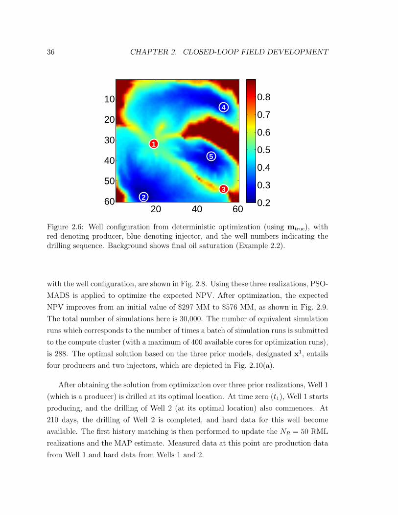
36 CHAPTER 2. CLOSED-LOOP FIELD DEVELOPMENT
2
4
5
1
3
20 40 60
10
20
30
40
50
60 0.2
0.3
0.4
0.5
0.6
0.7
0.8
Figure 2.6: Well configuration from deterministic optimization (using mtrue), withred denoting producer, blue denoting injector, and the well numbers indicating thedrilling sequence. Background shows final oil saturation (Example 2.2).
with the well configuration, are shown in Fig. 2.8. Using these three realizations, PSO-
MADS is applied to optimize the expected NPV. After optimization, the expected
NPV improves from an initial value of $297 MM to $576 MM, as shown in Fig. 2.9.
The total number of simulations here is 30,000. The number of equivalent simulation
runs which corresponds to the number of times a batch of simulation runs is submitted
to the compute cluster (with a maximum of 400 available cores for optimization runs),
is 288. The optimal solution based on the three prior models, designated x1, entails
four producers and two injectors, which are depicted in Fig. 2.10(a).
After obtaining the solution from optimization over three prior realizations, Well 1
(which is a producer) is drilled at its optimal location. At time zero (t1), Well 1 starts
producing, and the drilling of Well 2 (at its optimal location) also commences. At
210 days, the drilling of Well 2 is completed, and hard data for this well become
available. The first history matching is then performed to update the NR = 50 RML
realizations and the MAP estimate. Measured data at this point are production data
from Well 1 and hard data from Wells 1 and 2.
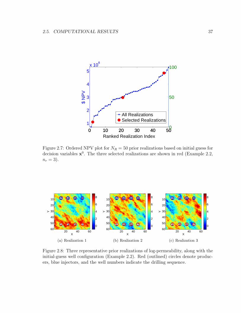
2.5. COMPUTATIONAL RESULTS 37
0 10 20 30 40 50
1
2
3
4
5x 10
8
$ N
PV
Ranked Realization Index
0 10 20 30 40 500
50
100
All RealizationsSelected Realizations
Figure 2.7: Ordered NPV plot for NR = 50 prior realizations based on initial guess fordecision variables x0. The three selected realizations are shown in red (Example 2.2,nr = 3).
X
Y
1
2
3
4
5
6
7
8
20 40 60
10
20
30
40
50
600
2
4
6
8
(a) Realization 1
X
Y
1
2
3
4
5
6
7
8
20 40 60
10
20
30
40
50
600
2
4
6
8
(b) Realization 2
X
Y
1
2
3
4
5
6
7
8
20 40 60
10
20
30
40
50
600
2
4
6
8
(c) Realization 3
Figure 2.8: Three representative prior realizations of log-permeability, along with theinitial-guess well configuration (Example 2.2). Red (outlined) circles denote produc-ers, blue injectors, and the well numbers indicate the drilling sequence.
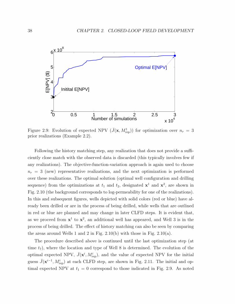
38 CHAPTER 2. CLOSED-LOOP FIELD DEVELOPMENT
0 0.5 1 1.5 2 2.5 3x 10
4
2
3
4
5
6x 10⁸
Number of simulations
E[N
PV
] ($)
Initital E[NPV]
Optimal E[NPV]
Figure 2.9: Evolution of expected NPV (J(x,M1rep)) for optimization over nr = 3
prior realizations (Example 2.2).
Following the history matching step, any realization that does not provide a suffi-
ciently close match with the observed data is discarded (this typically involves few if
any realizations). The objective-function-variation approach is again used to choose
nr = 3 (new) representative realizations, and the next optimization is performed
over these realizations. The optimal solution (optimal well configuration and drilling
sequence) from the optimizations at t1 and t2, designated x1 and x2, are shown in
Fig. 2.10 (the background corresponds to log-permeability for one of the realizations).
In this and subsequent figures, wells depicted with solid colors (red or blue) have al-
ready been drilled or are in the process of being drilled, while wells that are outlined
in red or blue are planned and may change in later CLFD steps. It is evident that,
as we proceed from x1 to x2, an additional well has appeared, and Well 3 is in the
process of being drilled. The effect of history matching can also be seen by comparing
the areas around Wells 1 and 2 in Fig. 2.10(b) with those in Fig. 2.10(a).
The procedure described above is continued until the last optimization step (at
time t7), where the location and type of Well 8 is determined. The evolution of the
optimal expected NPV, J(xi,M irep), and the value of expected NPV for the initial
guess J(xi−1,M irep) at each CLFD step, are shown in Fig. 2.11. The initial and op-
timal expected NPV at t1 = 0 correspond to those indicated in Fig. 2.9. As noted
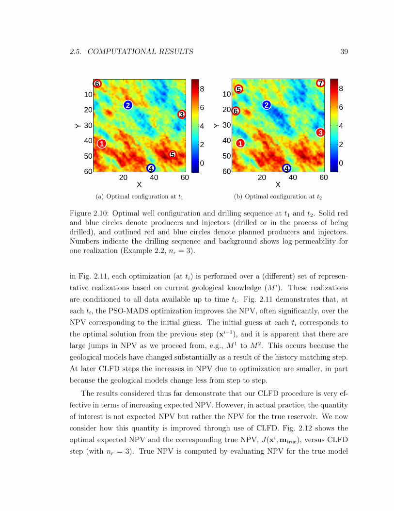
2.5. COMPUTATIONAL RESULTS 39
X
Y
1
23
4
5
6
20 40 60
10
20
30
40
50
600
2
4
6
8
(a) Optimal configuration at t1
X
Y
1
2
3
4
5
6
7
20 40 60
10
20
30
40
50
600
2
4
6
8
(b) Optimal configuration at t2
Figure 2.10: Optimal well configuration and drilling sequence at t1 and t2. Solid redand blue circles denote producers and injectors (drilled or in the process of beingdrilled), and outlined red and blue circles denote planned producers and injectors.Numbers indicate the drilling sequence and background shows log-permeability forone realization (Example 2.2, nr = 3).
in Fig. 2.11, each optimization (at ti) is performed over a (different) set of represen-
tative realizations based on current geological knowledge (M i). These realizations
are conditioned to all data available up to time ti. Fig. 2.11 demonstrates that, at
each ti, the PSO-MADS optimization improves the NPV, often significantly, over the
NPV corresponding to the initial guess. The initial guess at each ti corresponds to
the optimal solution from the previous step (xi−1), and it is apparent that there are
large jumps in NPV as we proceed from, e.g., M1 to M2. This occurs because the
geological models have changed substantially as a result of the history matching step.
At later CLFD steps the increases in NPV due to optimization are smaller, in part
because the geological models change less from step to step.
The results considered thus far demonstrate that our CLFD procedure is very ef-
fective in terms of increasing expected NPV. However, in actual practice, the quantity
of interest is not expected NPV but rather the NPV for the true reservoir. We now
consider how this quantity is improved through use of CLFD. Fig. 2.12 shows the
optimal expected NPV and the corresponding true NPV, J(xi,mtrue), versus CLFD
step (with nr = 3). True NPV is computed by evaluating NPV for the true model

40 CHAPTER 2. CLOSED-LOOP FIELD DEVELOPMENT
0 210 420 630 840 1050 12602
3
4
5
6x 10⁸
Time (Days)
NP
V (
$)
M1 M2 M3 M4 M5 M6 M7
J(xi−1,M i
rep)
J(xi,M i
rep)
Figure 2.11: Optimal expected NPV, J(xi,M irep), and the expected NPV for the
corresponding initial guess, J(xi−1,M irep), versus CLFD step (Example 2.2, nr = 3).
0 210 420 630 840 1050 12601
2
3
4
5
6
7
x 108
Time (Days)
NP
V (
$)
J(xi,M i
rep)
J(xi,mtrue)
DeterministicFinal NPV$ 398 MM
Figure 2.12: Optimal expected NPV, J(xi,M irep), and the corresponding NPV for the
true model, J(xi,mtrue), versus CLFD step. The star shows the final true NPV fromCLFD (Example 2.2, nr = 3).
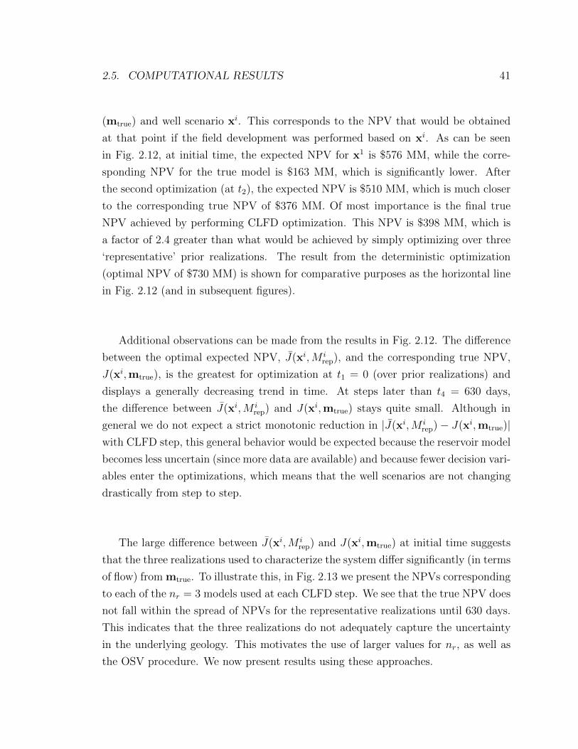
2.5. COMPUTATIONAL RESULTS 41
(mtrue) and well scenario xi. This corresponds to the NPV that would be obtained
at that point if the field development was performed based on xi. As can be seen
in Fig. 2.12, at initial time, the expected NPV for x1 is $576 MM, while the corre-
sponding NPV for the true model is $163 MM, which is significantly lower. After
the second optimization (at t2), the expected NPV is $510 MM, which is much closer
to the corresponding true NPV of $376 MM. Of most importance is the final true
NPV achieved by performing CLFD optimization. This NPV is $398 MM, which is
a factor of 2.4 greater than what would be achieved by simply optimizing over three
‘representative’ prior realizations. The result from the deterministic optimization
(optimal NPV of $730 MM) is shown for comparative purposes as the horizontal line
in Fig. 2.12 (and in subsequent figures).
Additional observations can be made from the results in Fig. 2.12. The difference
between the optimal expected NPV, J(xi,M irep), and the corresponding true NPV,
J(xi,mtrue), is the greatest for optimization at t1 = 0 (over prior realizations) and
displays a generally decreasing trend in time. At steps later than t4 = 630 days,
the difference between J(xi,M irep) and J(xi,mtrue) stays quite small. Although in
general we do not expect a strict monotonic reduction in |J(xi,M irep)− J(xi,mtrue)|
with CLFD step, this general behavior would be expected because the reservoir model
becomes less uncertain (since more data are available) and because fewer decision vari-
ables enter the optimizations, which means that the well scenarios are not changing
drastically from step to step.
The large difference between J(xi,M irep) and J(xi,mtrue) at initial time suggests
that the three realizations used to characterize the system differ significantly (in terms
of flow) from mtrue. To illustrate this, in Fig. 2.13 we present the NPVs corresponding
to each of the nr = 3 models used at each CLFD step. We see that the true NPV does
not fall within the spread of NPVs for the representative realizations until 630 days.
This indicates that the three realizations do not adequately capture the uncertainty
in the underlying geology. This motivates the use of larger values for nr, as well as
the OSV procedure. We now present results using these approaches.
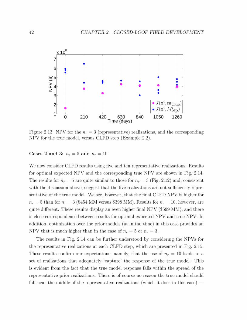
42 CHAPTER 2. CLOSED-LOOP FIELD DEVELOPMENT
0 210 420 630 840 1050 12601
2
3
4
5
6
7
x 108
Time (days)
NP
V (
$)
J(xi,mtrue)
J(xi, M i
rep)
Figure 2.13: NPV for the nr = 3 (representative) realizations, and the correspondingNPV for the true model, versus CLFD step (Example 2.2).
Cases 2 and 3: nr = 5 and nr = 10
We now consider CLFD results using five and ten representative realizations. Results
for optimal expected NPV and the corresponding true NPV are shown in Fig. 2.14.
The results for nr = 5 are quite similar to those for nr = 3 (Fig. 2.12) and, consistent
with the discussion above, suggest that the five realizations are not sufficiently repre-
sentative of the true model. We see, however, that the final CLFD NPV is higher for
nr = 5 than for nr = 3 ($454 MM versus $398 MM). Results for nr = 10, however, are
quite different. These results display an even higher final NPV ($599 MM), and there
is close correspondence between results for optimal expected NPV and true NPV. In
addition, optimization over the prior models (at initial time) in this case provides an
NPV that is much higher than in the case of nr = 5 or nr = 3.
The results in Fig. 2.14 can be further understood by considering the NPVs for
the representative realizations at each CLFD step, which are presented in Fig. 2.15.
These results confirm our expectations; namely, that the use of nr = 10 leads to a
set of realizations that adequately ‘capture’ the response of the true model. This
is evident from the fact that the true model response falls within the spread of the
representative prior realizations. There is of course no reason the true model should
fall near the middle of the representative realizations (which it does in this case) —

2.5. COMPUTATIONAL RESULTS 43
the key point is that the true realization does not appear as an outlier (as it does for
nr = 3 and nr = 5). We note finally that, even though the nr = 10 prior realizations
are representative of the true model, the use of CLFD still leads to an 18% increase
in NPV compared to that achieved by simply optimizing over the prior realizations.
The reduction in uncertainty using CLFD, as well as the ‘representivity’ of the
selected realizations, can be further assessed by evaluating the NPVs for the entire set
of (50) current realizations with the current optimal solution xi. Fig. 2.16 presents
the P10–P50–P90 results for NPV, determined by simulating all 50 realizations and
then constructing the cdf, at each control step for nr = 5 and nr = 10. The expected
NPV based on the current representative set is also displayed. It is evident that for
nr = 5, the optimal expected NPV for the representative set falls outside of the P10–
P90 range at the first three CLFD steps (Fig. 2.16(a)). For nr = 10, by contrast,
the optimal expected NPV for the representative set always falls within the P10–P90
range. The generally decreasing trend in the P10–P90 range with increasing CLFD
step, apparent for both nr = 5 and nr = 10, highlights the reduction in uncertainty
achieved through application of CLFD.
In order to better quantify the performance of CLFD, we performed two additional
runs, with different mtrue, using both nr = 5 and nr = 10. For the mtrue considered
above, and for these two new cases, we also optimized over all 50 prior models and
then applied the optimal well configuration and controls to the true model. This
computation essentially represents the ‘most robust’ optimization we can perform
using only (the 50) prior models. Results for all of these computations are presented
in Table 2.3 (the first row corresponds to the true model considered above). From
the table, we see that the use of CLFD in all cases (even using nr = 5) provides
higher NPVs than does optimizing over 50 prior realizations. In addition, CLFD
with nr = 10 consistently outperforms CLFD with nr = 5. In fact, CLFD with
nr = 10 leads to improvements in NPV ranging from 45% to 71% over those achieved
by optimizing over 50 prior realizations.
Case 4: Use of optimization with sample validation
The results thus far suggest that the use of nr = 10 in CLFD is adequate, but nr =
3 or 5 is insufficient. In general, however, the appropriate value to use for nr is not
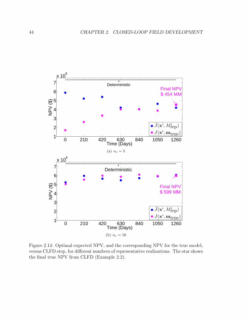
44 CHAPTER 2. CLOSED-LOOP FIELD DEVELOPMENT
0 210 420 630 840 1050 12601
2
3
4
5
6
7x 10
8
Time (Days)
NP
V (
$)
J(xi,M i
rep)
J(xi,mtrue)
DeterministicFinal NPV$ 454 MM
(a) nr = 5
0 210 420 630 840 1050 12601
2
3
4
5
6
7x 10
8
Time (Days)
NP
V (
$)
J(xi,M i
rep)
J(xi,mtrue)
Deterministic
Final NPV$ 599 MM
(b) nr = 10
Figure 2.14: Optimal expected NPV, and the corresponding NPV for the true model,versus CLFD step, for different numbers of representative realizations. The star showsthe final true NPV from CLFD (Example 2.2).
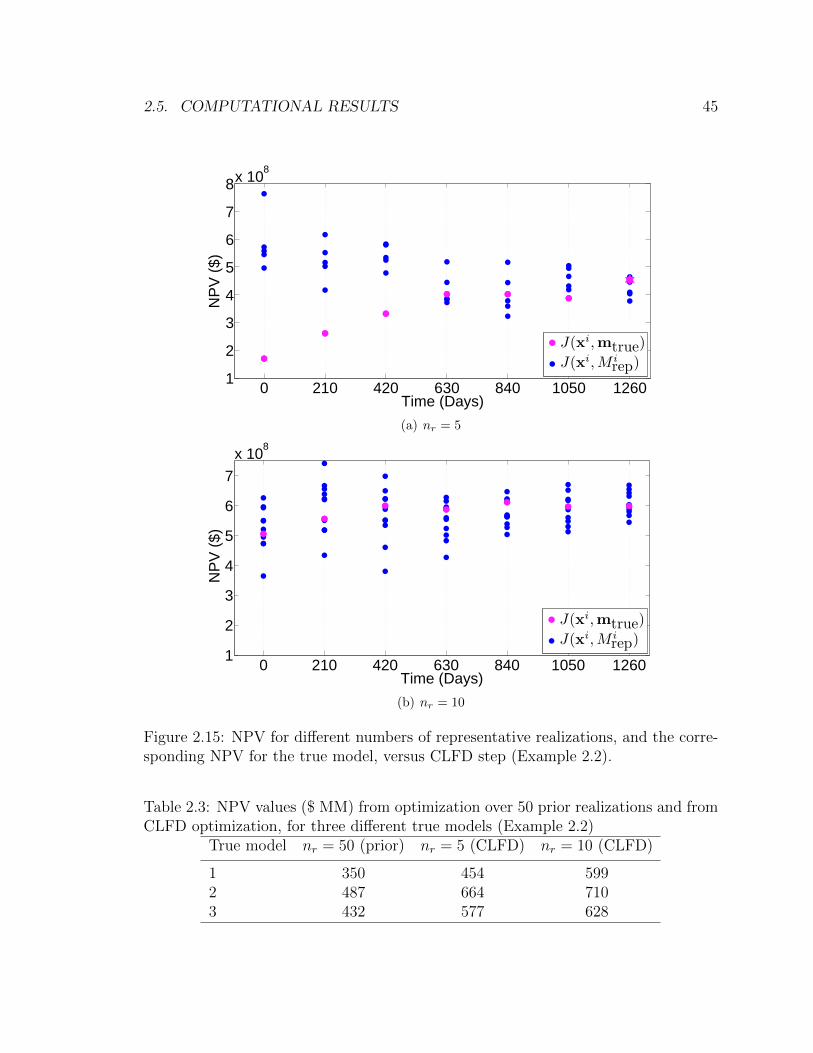
2.5. COMPUTATIONAL RESULTS 45
0 210 420 630 840 1050 12601
2
3
4
5
6
7
8x 10⁸
Time (Days)
NP
V (
$)
J(xi,mtrue)
J(xi, M i
rep)
(a) nr = 5
0 210 420 630 840 1050 12601
2
3
4
5
6
7
x 108
Time (Days)
NP
V (
$)
J(xi,mtrue)
J(xi, M i
rep)
(b) nr = 10
Figure 2.15: NPV for different numbers of representative realizations, and the corre-sponding NPV for the true model, versus CLFD step (Example 2.2).
Table 2.3: NPV values ($ MM) from optimization over 50 prior realizations and fromCLFD optimization, for three different true models (Example 2.2)
True model nr = 50 (prior) nr = 5 (CLFD) nr = 10 (CLFD)
1 350 454 5992 487 664 7103 432 577 628
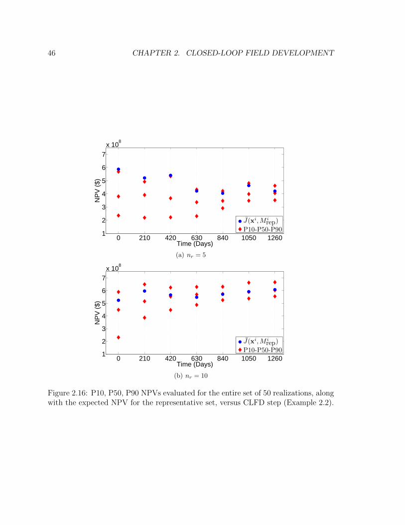
46 CHAPTER 2. CLOSED-LOOP FIELD DEVELOPMENT
0 210 420 630 840 1050 12601
2
3
4
5
6
7
x 108
Time (Days)
NP
V (
$)
J(xi,M irep)
P10-P50-P90
(a) nr = 5
0 210 420 630 840 1050 12601
2
3
4
5
6
7x 10
8
Time (Days)
NP
V (
$)
J(xi,M irep)
P10-P50-P90
(b) nr = 10
Figure 2.16: P10, P50, P90 NPVs evaluated for the entire set of 50 realizations, alongwith the expected NPV for the representative set, versus CLFD step (Example 2.2).
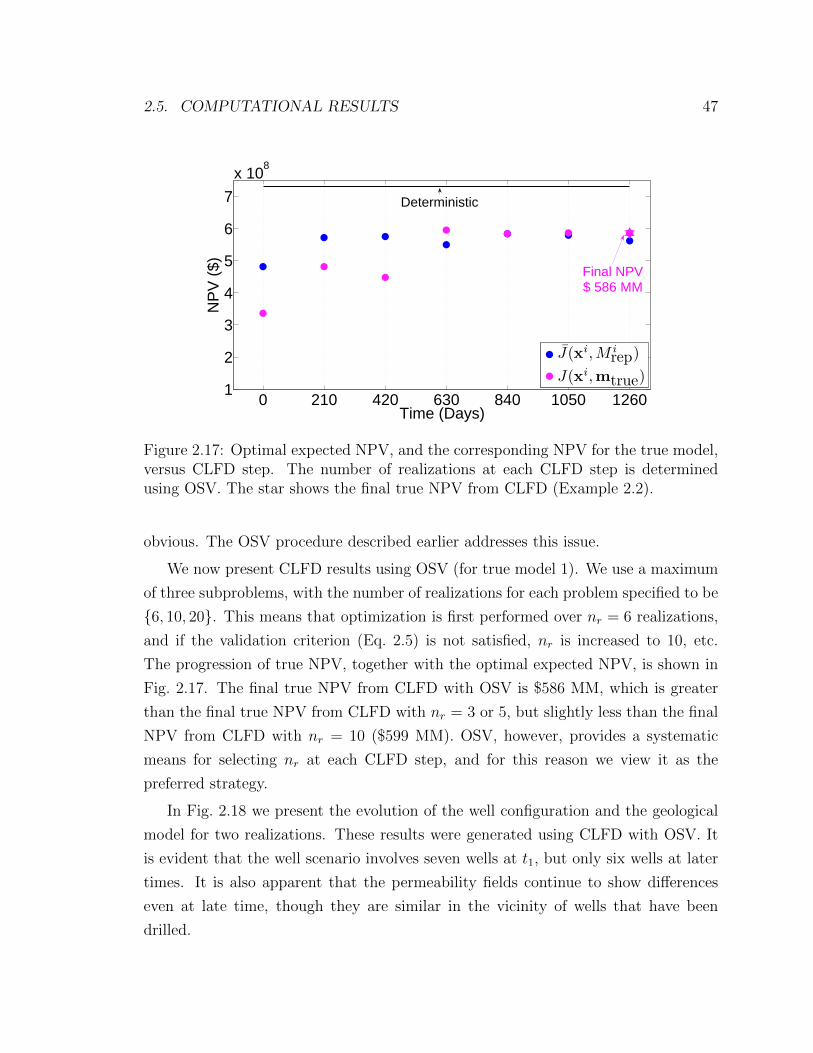
2.5. COMPUTATIONAL RESULTS 47
0 210 420 630 840 1050 12601
2
3
4
5
6
7
x 108
Time (Days)
NP
V (
$)
J(xi,M i
rep)
J(xi,mtrue)
Final NPV$ 586 MM
Deterministic
Figure 2.17: Optimal expected NPV, and the corresponding NPV for the true model,versus CLFD step. The number of realizations at each CLFD step is determinedusing OSV. The star shows the final true NPV from CLFD (Example 2.2).
obvious. The OSV procedure described earlier addresses this issue.
We now present CLFD results using OSV (for true model 1). We use a maximum
of three subproblems, with the number of realizations for each problem specified to be
{6, 10, 20}. This means that optimization is first performed over nr = 6 realizations,
and if the validation criterion (Eq. 2.5) is not satisfied, nr is increased to 10, etc.
The progression of true NPV, together with the optimal expected NPV, is shown in
Fig. 2.17. The final true NPV from CLFD with OSV is $586 MM, which is greater
than the final true NPV from CLFD with nr = 3 or 5, but slightly less than the final
NPV from CLFD with nr = 10 ($599 MM). OSV, however, provides a systematic
means for selecting nr at each CLFD step, and for this reason we view it as the
preferred strategy.
In Fig. 2.18 we present the evolution of the well configuration and the geological
model for two realizations. These results were generated using CLFD with OSV. It
is evident that the well scenario involves seven wells at t1, but only six wells at later
times. It is also apparent that the permeability fields continue to show differences
even at late time, though they are similar in the vicinity of wells that have been
drilled.
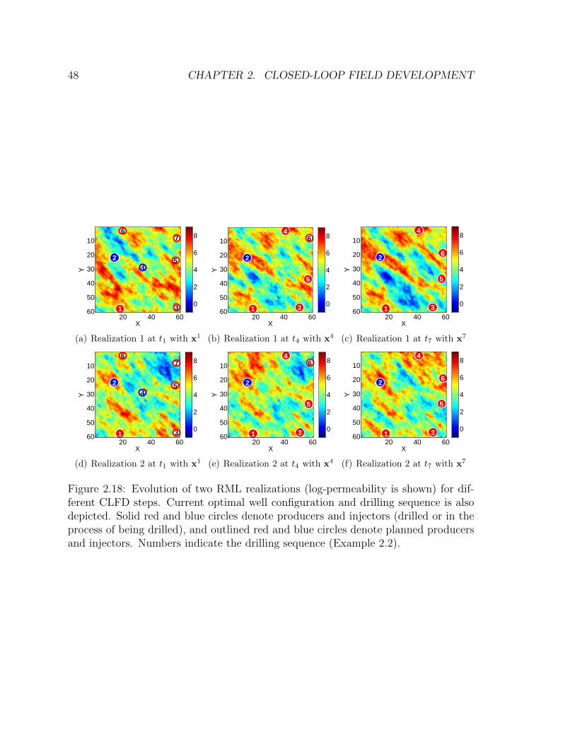
48 CHAPTER 2. CLOSED-LOOP FIELD DEVELOPMENT
X
Y
1
2
3
45
67
20 40 60
10
20
30
40
50
600
2
4
6
8
(a) Realization 1 at t1 with x1
X
Y
1
2
3
4
5
6
20 40 60
10
20
30
40
50
600
2
4
6
8
(b) Realization 1 at t4 with x4
X
Y
1
2
3
4
5
6
20 40 60
10
20
30
40
50
600
2
4
6
8
(c) Realization 1 at t7 with x7
X
Y
1
2
3
45
67
20 40 60
10
20
30
40
50
600
2
4
6
8
(d) Realization 2 at t1 with x1
X
Y
1
2
3
4
5
6
20 40 60
10
20
30
40
50
600
2
4
6
8
(e) Realization 2 at t4 with x4
X
Y
1
2
3
4
5
6
20 40 60
10
20
30
40
50
600
2
4
6
8
(f) Realization 2 at t7 with x7
Figure 2.18: Evolution of two RML realizations (log-permeability is shown) for dif-ferent CLFD steps. Current optimal well configuration and drilling sequence is alsodepicted. Solid red and blue circles denote producers and injectors (drilled or in theprocess of being drilled), and outlined red and blue circles denote planned producersand injectors. Numbers indicate the drilling sequence (Example 2.2).
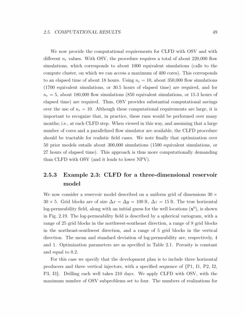
2.5. COMPUTATIONAL RESULTS 49
We now provide the computational requirements for CLFD with OSV and with
different nr values. With OSV, the procedure requires a total of about 220,000 flow
simulations, which corresponds to about 1000 equivalent simulations (calls to the
compute cluster, on which we can access a maximum of 400 cores). This corresponds
to an elapsed time of about 18 hours. Using nr = 10, about 350,000 flow simulations
(1700 equivalent simulations, or 30.5 hours of elapsed time) are required, and for
nr = 5, about 180,000 flow simulations (850 equivalent simulations, or 15.3 hours of
elapsed time) are required. Thus, OSV provides substantial computational savings
over the use of nr = 10. Although these computational requirements are large, it is
important to recognize that, in practice, these runs would be performed over many
months; i.e., at each CLFD step. When viewed in this way, and assuming that a large
number of cores and a parallelized flow simulator are available, the CLFD procedure
should be tractable for realistic field cases. We note finally that optimization over
50 prior models entails about 300,000 simulations (1500 equivalent simulations, or
27 hours of elapsed time). This approach is thus more computationally demanding
than CLFD with OSV (and it leads to lower NPV).
2.5.3 Example 2.3: CLFD for a three-dimensional reservoir
model
We now consider a reservoir model described on a uniform grid of dimensions 30 ×30 × 5. Grid blocks are of size ∆x = ∆y = 100 ft, ∆z = 15 ft. The true horizontal
log-permeability field, along with an initial guess for the well locations (x0), is shown
in Fig. 2.19. The log-permeability field is described by a spherical variogram, with a
range of 25 grid blocks in the northwest-southeast direction, a range of 8 grid blocks
in the northeast-southwest direction, and a range of 5 grid blocks in the vertical
direction. The mean and standard deviation of log-permeability are, respectively, 4
and 1. Optimization parameters are as specified in Table 2.1. Porosity is constant
and equal to 0.2.
For this case we specify that the development plan is to include three horizontal
producers and three vertical injectors, with a specified sequence of {P1, I1, P2, I2,
P3, I3}. Drilling each well takes 210 days. We apply CLFD with OSV, with the
maximum number of OSV subproblems set to four. The numbers of realizations for
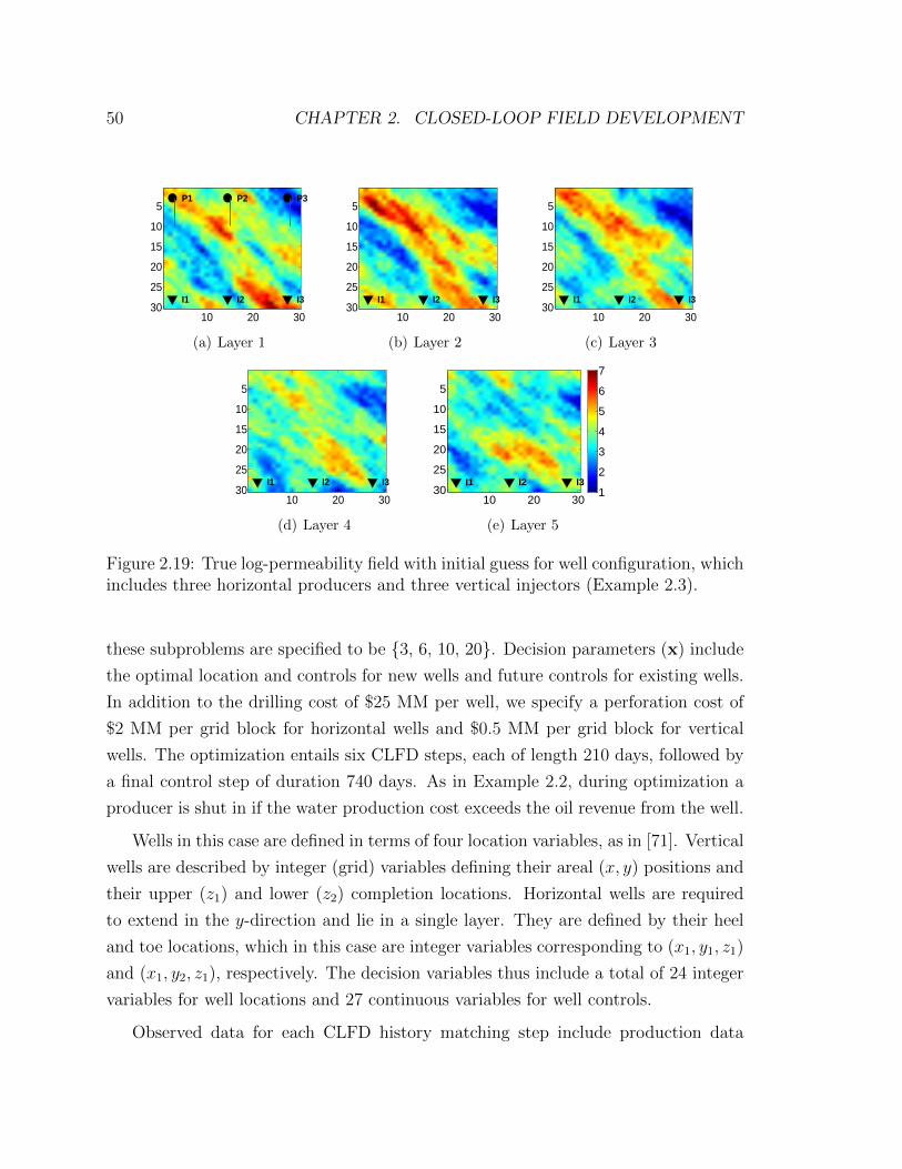
50 CHAPTER 2. CLOSED-LOOP FIELD DEVELOPMENT
P1
I1
P2
I2
P3
I3
10 20 30
5
10
15
20
25
30
(a) Layer 1
I1 I2 I3
10 20 30
5
10
15
20
25
30
(b) Layer 2
I1 I2 I3
10 20 30
5
10
15
20
25
30
(c) Layer 3
I1 I2 I3
10 20 30
5
10
15
20
25
30
(d) Layer 4
I1 I2 I3
10 20 30
5
10
15
20
25
30 1
2
3
4
5
6
7
(e) Layer 5
Figure 2.19: True log-permeability field with initial guess for well configuration, whichincludes three horizontal producers and three vertical injectors (Example 2.3).
these subproblems are specified to be {3, 6, 10, 20}. Decision parameters (x) include
the optimal location and controls for new wells and future controls for existing wells.
In addition to the drilling cost of $25 MM per well, we specify a perforation cost of
$2 MM per grid block for horizontal wells and $0.5 MM per grid block for vertical
wells. The optimization entails six CLFD steps, each of length 210 days, followed by
a final control step of duration 740 days. As in Example 2.2, during optimization a
producer is shut in if the water production cost exceeds the oil revenue from the well.
Wells in this case are defined in terms of four location variables, as in [71]. Vertical
wells are described by integer (grid) variables defining their areal (x, y) positions and
their upper (z1) and lower (z2) completion locations. Horizontal wells are required
to extend in the y-direction and lie in a single layer. They are defined by their heel
and toe locations, which in this case are integer variables corresponding to (x1, y1, z1)
and (x1, y2, z1), respectively. The decision variables thus include a total of 24 integer
variables for well locations and 27 continuous variables for well controls.
Observed data for each CLFD history matching step include production data

2.5. COMPUTATIONAL RESULTS 51
0 210 420 630 8407
7.5
8
8.5
9
9.5x 10⁸
Time (Days)
NP
V (
$)
J(xi,M i
rep)
J(xi,mtrue)
Deterministic
Final NPV$ 899 MM
Figure 2.20: Optimal expected NPV, and the corresponding NPV for the true model,versus CLFD step. The number of realizations at each CLFD step is determinedusing OSV. The star shows the final true NPV from CLFD (Example 2.3).
measured at 30-day intervals and hard data from all existing wells. Observed data
types and measurement errors are analogous to those for Example 2.2. We assume
that hard data are available for all perforated grid blocks. Model parameters for
history matching include horizontal log-permeabilities for all grid blocks. The ratio
of vertical permeability to horizontal permeability (kz/kh) is specified to be 0.2 and
is assumed to be known.
We first apply deterministic optimization (using the true model) for this problem,
which gives an optimal NPV of $941 MM. The progress of optimal expected NPV and
true NPV, as a function of CLFD step, is shown in Fig. 2.20. The deterministic result
appears as the horizontal line. CLFD performs quite well in this case, and achieves
a final NPV of $899 MM, which is close to the deterministic result. Although there
is an offset in Fig. 2.20 between true and expected NPV in the first two CLFD steps,
the value of this offset is not large (note the relatively small NPV range on the y-axis
in Fig. 2.20). The application of CLFD with OSV provides about a 20% improvement
in the true NPV over the NPV achieved from optimization over the prior realizations.
For this example, we again optimize over all 50 prior realizations in order to
compare CLFD results with those from robust optimization over prior models. The
expected NPV over the 50 prior realizations is $878 MM, but the NPV for the true
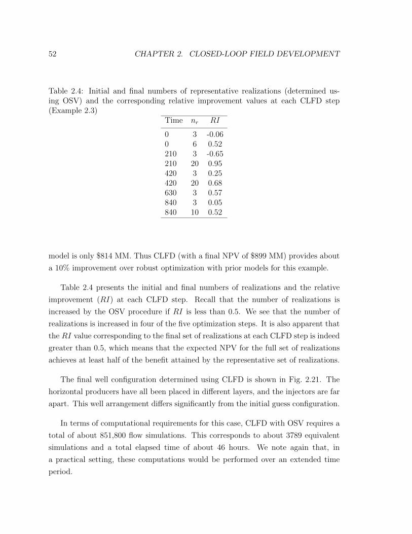
52 CHAPTER 2. CLOSED-LOOP FIELD DEVELOPMENT
Table 2.4: Initial and final numbers of representative realizations (determined us-ing OSV) and the corresponding relative improvement values at each CLFD step(Example 2.3)
Time nr RI
0 3 -0.060 6 0.52210 3 -0.65210 20 0.95420 3 0.25420 20 0.68630 3 0.57840 3 0.05840 10 0.52
model is only $814 MM. Thus CLFD (with a final NPV of $899 MM) provides about
a 10% improvement over robust optimization with prior models for this example.
Table 2.4 presents the initial and final numbers of realizations and the relative
improvement (RI) at each CLFD step. Recall that the number of realizations is
increased by the OSV procedure if RI is less than 0.5. We see that the number of
realizations is increased in four of the five optimization steps. It is also apparent that
the RI value corresponding to the final set of realizations at each CLFD step is indeed
greater than 0.5, which means that the expected NPV for the full set of realizations
achieves at least half of the benefit attained by the representative set of realizations.
The final well configuration determined using CLFD is shown in Fig. 2.21. The
horizontal producers have all been placed in different layers, and the injectors are far
apart. This well arrangement differs significantly from the initial guess configuration.
In terms of computational requirements for this case, CLFD with OSV requires a
total of about 851,800 flow simulations. This corresponds to about 3789 equivalent
simulations and a total elapsed time of about 46 hours. We note again that, in
a practical setting, these computations would be performed over an extended time
period.
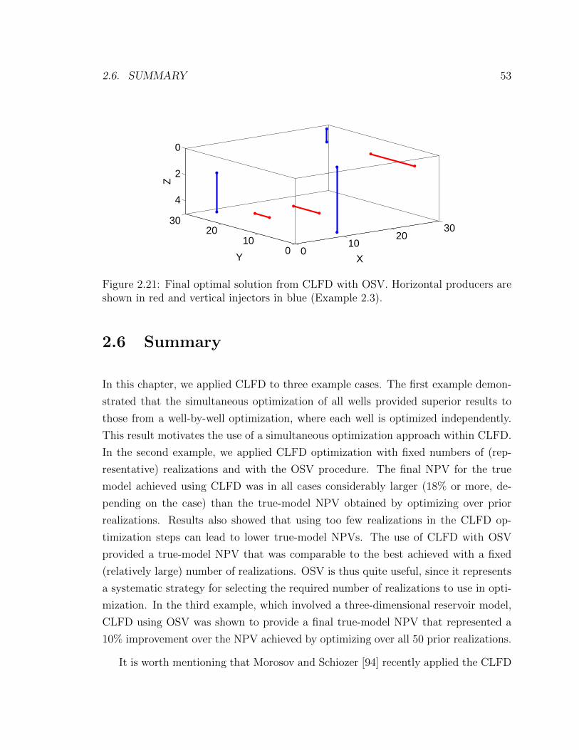
2.6. SUMMARY 53
010
2030
010
2030
0
2
4
XY
Z
Figure 2.21: Final optimal solution from CLFD with OSV. Horizontal producers areshown in red and vertical injectors in blue (Example 2.3).
2.6 Summary
In this chapter, we applied CLFD to three example cases. The first example demon-
strated that the simultaneous optimization of all wells provided superior results to
those from a well-by-well optimization, where each well is optimized independently.
This result motivates the use of a simultaneous optimization approach within CLFD.
In the second example, we applied CLFD optimization with fixed numbers of (rep-
resentative) realizations and with the OSV procedure. The final NPV for the true
model achieved using CLFD was in all cases considerably larger (18% or more, de-
pending on the case) than the true-model NPV obtained by optimizing over prior
realizations. Results also showed that using too few realizations in the CLFD op-
timization steps can lead to lower true-model NPVs. The use of CLFD with OSV
provided a true-model NPV that was comparable to the best achieved with a fixed
(relatively large) number of realizations. OSV is thus quite useful, since it represents
a systematic strategy for selecting the required number of realizations to use in opti-
mization. In the third example, which involved a three-dimensional reservoir model,
CLFD using OSV was shown to provide a final true-model NPV that represented a
10% improvement over the NPV achieved by optimizing over all 50 prior realizations.
It is worth mentioning that Morosov and Schiozer [94] recently applied the CLFD

54 CHAPTER 2. CLOSED-LOOP FIELD DEVELOPMENT
framework to a realistic example. They used different reservoir modeling and dif-
ferent history matching and optimization approaches in their CLFD application. In
particular, they applied ensemble-based data assimilation (ES-MDA) [40] for history
matching. In their optimization step, nine representative models were selected, and
each model was optimized independently, resulting in nine different optimal solutions,
from which the solution that provided the highest expected NPV for the full set was
applied. Due to the complexity of the reservoir model, the history matching proce-
dure was not effective in providing appropriate uncertainty quantification, and this
caused the true model NPV to fall outside of the uncertainty range. The expected
NPV, however, increased by 29%.
The need for representative realizations in the CLFD optimization step motivated
us to further pursue the subject of selection of representative models. In this chapter,
representative models were selected based on a ranking of NPVs. In Chapter 3,
we will investigate more sophisticated procedures that consider a combination of
flow quantities and static (e.g., permeability field) information for the selection of
representative models.
We note finally that, in the CLFD framework presented in this chapter, the project
life was specified a priori. This is the usual approach taken in the reservoir optimiza-
tion literature. In Chapter 4 we will demonstrate that project life should also be
treated as an optimization variable. There, we investigate the joint optimization of
economic project life and well controls for a set of existing wells. Determination of
optimal project life for the field development optimization problem in CLFD is left
as future work.
Chapter 3
Selection of Representative Models
for Decision Making and
Optimization Under Uncertainty
In this chapter, we address the realization-selection problem systematically. Toward
this end, we first describe a procedure for quantitatively assessing different approaches
using a flow-response variable. We then introduce a general clustering method for
the selection of representative realizations. In this clustering, each realization is
represented by a feature vector composed of a weighted combination of flow-based
and geological quantities. Principal component analysis (PCA) is used to express
the geology (permeability field) in terms of a small number of features, while flow-
based features are obtained by solving one or more flow problems. The use of both
full-physics simulations and efficient tracer-type simulations for obtaining these flow-
based features is considered. We then investigate the performance of different feature
weightings for problems involving new well locations or new well controls, with the
goal of identifying the selection method that provides the ‘best’ subsets of realizations
(meaning that the flow response computed for a subset is in close agreement with that
for the full set). Finally, the performance of various methods will be assessed for a
well control optimization problem. Additional results, involving binary channelized
models, are presented in Appendix B.
55

56 CHAPTER 3. SELECTION OF REPRESENTATIVE MODELS
3.1 Assessment of flow-response statistics for a rep-
resentative subset
In this section, we define the flow-response vector, r, and we then describe an ap-
proach for comparing different selection methods based on flow responses. We let
the Nm-dimensional vector mj designate a geological realization of the model, which
contains as its elements the grid block log-permeability values (where j is the real-
ization index). The matrix Mfull designates the full set of geological models, Mfull =
[m1 m2 . . . mNR]. The NR realizations of mj typically correspond to a sampling
from a probability distribution. Our interest is to define a low-dimensional vector r
that captures the flow response of realization mj for a given x, where x defines the
well configuration (here we consider x−y spatial locations) and control (time-varying
bottom-hole pressure or BHP) parameters. We also refer to x as the well-parameter
vector or the vector of decision parameters.
For realization mj and well-parameter vector x, we define rj as
rj(x,mj) = [q1j ,q
2j , . . .q
nwj ]T , (3.1)
where qkj , k = 1, . . . , nw is a row vector of incremental phase production/injection
data for well k, and nw designates the number of wells. The vector qkj is referred to
as the well flow response. To compute qkj , the reservoir life is divided into a relatively
small number of time intervals, nt. By specifying a small number of time intervals,
the continuous flow response for a realization can be captured with a low-dimensional
vector. For a production well, qkj contains the total production for each phase (oil
and water in this chapter) at each time interval for the well, while for an injection
well, qkj includes the total water injected at each time interval. With nt = 3, for
example, qkj for a producer well is expressed as
qkj = [Qko,1, Q
ko,2, Q
ko,3, Q
kw,1, Q
kw,2, Q
kw,3], (3.2)
where Qko,1 and Qk
w,1, respectively, denote the total oil and water production for well
k in realization j during the first time interval, Qko,2 and Qk
w,2 are the corresponding
quantities for the second time interval, etc. Fig. 3.1 defines Qko components for a
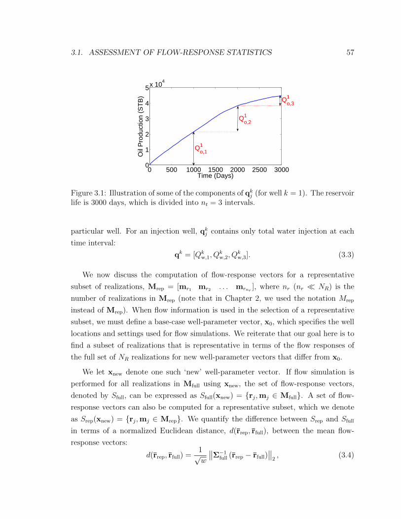
3.1. ASSESSMENT OF FLOW-RESPONSE STATISTICS 57
0 500 1000 1500 2000 2500 30000
1
2
3
4
5x 10⁴
Time (Days)
Oil
Pro
duct
ion
(ST
B)
Qo,11
Qo,21
Qo,31
Figure 3.1: Illustration of some of the components of qkj (for well k = 1). The reservoirlife is 3000 days, which is divided into nt = 3 intervals.
particular well. For an injection well, qkj contains only total water injection at each
time interval:
qk = [Qkw,1, Q
kw,2, Q
kw,3]. (3.3)
We now discuss the computation of flow-response vectors for a representative
subset of realizations, Mrep = [mr1 mr2 . . . mrnr], where nr (nr � NR) is the
number of realizations in Mrep (note that in Chapter 2, we used the notation Mrep
instead of Mrep). When flow information is used in the selection of a representative
subset, we must define a base-case well-parameter vector, x0, which specifies the well
locations and settings used for flow simulations. We reiterate that our goal here is to
find a subset of realizations that is representative in terms of the flow responses of
the full set of NR realizations for new well-parameter vectors that differ from x0.
We let xnew denote one such ‘new’ well-parameter vector. If flow simulation is
performed for all realizations in Mfull using xnew, the set of flow-response vectors,
denoted by Sfull, can be expressed as Sfull(xnew) = {rj,mj ∈ Mfull}. A set of flow-
response vectors can also be computed for a representative subset, which we denote
as Srep(xnew) = {rj,mj ∈ Mrep}. We quantify the difference between Srep and Sfull
in terms of a normalized Euclidean distance, d(rrep, rfull), between the mean flow-
response vectors:
d(rrep, rfull) =1√w
∥∥Σ−1full (rrep − rfull)
∥∥2, (3.4)

58 CHAPTER 3. SELECTION OF REPRESENTATIVE MODELS
where w is the dimension of the flow-response vector and Σfull is a diagonal matrix
with each diagonal entry equal to the standard deviation of the corresponding element
of the flow-response vector computed from the full set of realizations. A smaller value
of d(rrep, rfull), which we will refer to as ‘dissimilarity,’ is desirable as it corresponds to
a smaller difference between the mean flow response for the full set and that for the
representative subset of realizations. We note that other measures of dissimilarity
could also be used if particular flow-response statistics (e.g., P25) are of specific
interest.
We can now state the problem of realization selection more formally as follows.
Given a reference set Mfull of NR realizations, we seek a subset Mrep of size nr whose
mean flow-response vector rrep is as close as possible to the mean flow-response vector
of the full set, rfull, for a new well-parameter vector, xnew. In our case there are usually
many possible xnew, and these are often unknown a priori, which introduces additional
complication.
There are essentially an infinite number of possible new decision vectors xnew
that could be considered, so it is necessary to limit their range in our assessments.
In this regard, we first assume that our realization selection is being performed in
the context of a particular optimization problem and/or decision-making framework.
This will specify, or at least constrain, parameters such as the number and types of
wells, minimum well-to-well distances, bounds for well rates or BHPs, etc. To further
focus the range of xnew, we additionally consider the types of searches commonly used
in reservoir optimization algorithms. As discussed in Chapter 1, these optimizations
typically employ search steps that are either global and stochastic (e.g., GA and PSO
algorithms) or local and deterministic (pattern search or gradient-based algorithms).
The PSO–MADS algorithm used in all of the optimizations in Chapter 2 combines
both types of searches.
We thus consider well-parameter vectors xnew that correspond to these two types
of ‘moves.’ Specifically, we will assess the performance of various realization-selection
methods for sets of xnew that correspond to (1) large (random) global shifts, and (2)
small local shifts in well parameters relative to x0. In PSO and GA well placement
optimization algorithms, for example, many (in fact, nearly all at early iterations) of
the configurations considered are essentially random, perhaps subject to a minimum
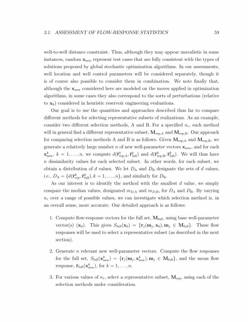
3.1. ASSESSMENT OF FLOW-RESPONSE STATISTICS 59
well-to-well distance constraint. Thus, although they may appear unrealistic in some
instances, random xnew represent test cases that are fully consistent with the types of
solutions proposed by global stochastic optimization algorithms. In our assessments,
well location and well control parameters will be considered separately, though it
is of course also possible to consider them in combination. We note finally that,
although the xnew considered here are modeled on the moves applied in optimization
algorithms, in some cases they also correspond to the sorts of perturbations (relative
to x0) considered in heuristic reservoir engineering evaluations.
Our goal is to use the quantities and approaches described thus far to compare
different methods for selecting representative subsets of realizations. As an example,
consider two different selection methods, A and B. For a specified nr, each method
will in general find a different representative subset, Mrep,A and Mrep,B. Our approach
for comparing selection methods A and B is as follows. Given Mrep,A and Mrep,B, we
generate a relatively large number n of new well-parameter vectors xnew, and for each
xknew, k = 1, . . . , n, we compute d(rkrep,A, rkfull) and d(rkrep,B, r
kfull). We will thus have
n dissimilarity values for each selected subset. In other words, for each subset, we
obtain a distribution of d values. We let DA and DB designate the sets of d values,
i.e., DA = {d(rkrep, rkfull), k = 1, . . . , n}, and similarly for DB.
As our interest is to identify the method with the smallest d value, we simply
compare the median values, designated mD,A and mD,B, for DA and DB. By varying
nr over a range of possible values, we can investigate which selection method is, in
an overall sense, more accurate. Our detailed approach is as follows:
1. Compute flow-response vectors for the full set, Mfull, using base well-parameter
vector(s) (x0). This gives Sfull(x0) = {rj(mj,x0),mj ∈ Mfull}. These flow
responses will be used to select a representative subset (as described in the next
section).
2. Generate n relevant new well-parameter vectors. Compute the flow responses
for the full set, Sfull(xknew) = {rj(mj,x
knew),mj ∈ Mfull}, and the mean flow
response, rfull(xknew), for k = 1, . . . , n.
3. For various values of nr, select a representative subset, Mrep, using each of the
selection methods under consideration.

60 CHAPTER 3. SELECTION OF REPRESENTATIVE MODELS
4. For each Mrep, compute the mean flow response for each of the n new well-
parameter vectors, and then compute d values.
5. Report the set of dissimilarity values, D = {d(rkrep, rkfull), k = 1, . . . , n}, and its
median, mD, for each Mrep.
6. For each nr, rank the selection methods, with the best method corresponding
to that with the smallest mD value.
3.2 Unsupervised learning for selecting a repre-
sentative subset
In this work, we consider uncertainty in only the permeability field. All other sys-
tem parameters are considered to be known, though our framework could be readily
generalized to treat uncertainty in other quantities. Our goal is to select nr repre-
sentative realizations from a large set of NR models. The selected realizations will
then be used to provide ‘representative’ flow simulation results for a wide range of
(currently unknown) new decision parameter vectors. Our selection method involves
a two-stage clustering approach. In the first stage, k-means clustering is applied to
divide the NR realizations into nr clusters, such that realizations in each cluster cor-
respond to similar features. In the second stage, k-medoids clustering is applied to
select one representative realization from each cluster (an alternate approach involv-
ing only k-medoids clustering will also be assessed). Prior to clustering, a feature
matrix is constructed, with each realization represented by a feature vector. We first
discuss our approach for generating the feature matrix (which contains the NR feature
vectors as columns), followed by a description of the detailed selection algorithm.
3.2.1 Feature selection
Selection of appropriate features/attributes is essential to the success of the over-
all methodology, and different features may be more or less relevant depending on
the problem. In the clustering procedure, an NR × NR (symmetric) distance ma-
trix is constructed from the feature vectors. Because each attribute influences the
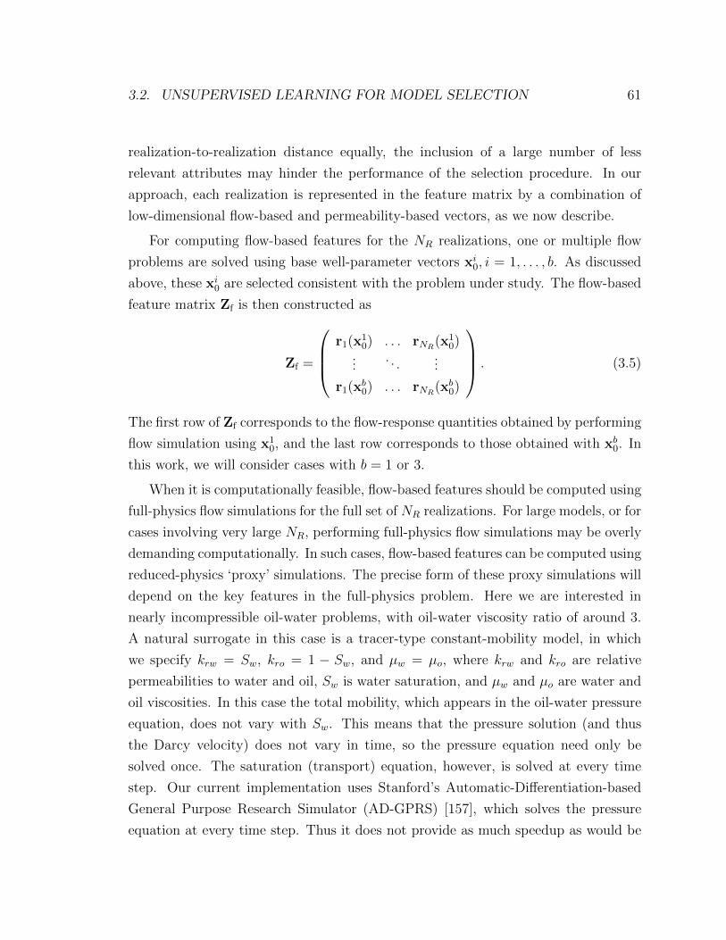
3.2. UNSUPERVISED LEARNING FOR MODEL SELECTION 61
realization-to-realization distance equally, the inclusion of a large number of less
relevant attributes may hinder the performance of the selection procedure. In our
approach, each realization is represented in the feature matrix by a combination of
low-dimensional flow-based and permeability-based vectors, as we now describe.
For computing flow-based features for the NR realizations, one or multiple flow
problems are solved using base well-parameter vectors xi0, i = 1, . . . , b. As discussed
above, these xi0 are selected consistent with the problem under study. The flow-based
feature matrix Zf is then constructed as
Zf =
r1(x
10) . . . rNR
(x10)
.... . .
...
r1(xb0) . . . rNR
(xb0)
. (3.5)
The first row of Zf corresponds to the flow-response quantities obtained by performing
flow simulation using x10, and the last row corresponds to those obtained with xb0. In
this work, we will consider cases with b = 1 or 3.
When it is computationally feasible, flow-based features should be computed using
full-physics flow simulations for the full set of NR realizations. For large models, or for
cases involving very large NR, performing full-physics flow simulations may be overly
demanding computationally. In such cases, flow-based features can be computed using
reduced-physics ‘proxy’ simulations. The precise form of these proxy simulations will
depend on the key features in the full-physics problem. Here we are interested in
nearly incompressible oil-water problems, with oil-water viscosity ratio of around 3.
A natural surrogate in this case is a tracer-type constant-mobility model, in which
we specify krw = Sw, kro = 1 − Sw, and µw = µo, where krw and kro are relative
permeabilities to water and oil, Sw is water saturation, and µw and µo are water and
oil viscosities. In this case the total mobility, which appears in the oil-water pressure
equation, does not vary with Sw. This means that the pressure solution (and thus
the Darcy velocity) does not vary in time, so the pressure equation need only be
solved once. The saturation (transport) equation, however, is solved at every time
step. Our current implementation uses Stanford’s Automatic-Differentiation-based
General Purpose Research Simulator (AD-GPRS) [157], which solves the pressure
equation at every time step. Thus it does not provide as much speedup as would be
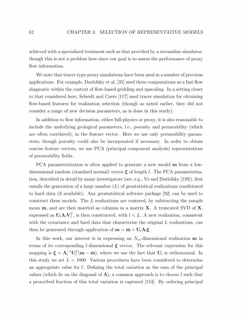
62 CHAPTER 3. SELECTION OF REPRESENTATIVE MODELS
achieved with a specialized treatment such as that provided by a streamline simulator,
though this is not a problem here since our goal is to assess the performance of proxy
flow information.
We note that tracer-type proxy simulations have been used in a number of previous
applications. For example, Durlofsky et al. [35] used these computations as a fast flow
diagnostic within the context of flow-based gridding and upscaling. In a setting closer
to that considered here, Scheidt and Caers [117] used tracer simulation for obtaining
flow-based features for realization selection (though as noted earlier, they did not
consider a range of new decision parameters, as is done in this study).
In addition to flow information, either full-physics or proxy, it is also reasonable to
include the underlying geological parameters, i.e., porosity and permeability (which
are often correlated), in the feature vector. Here we use only permeability param-
eters, though porosity could also be incorporated if necessary. In order to obtain
concise feature vectors, we use PCA (principal component analysis) representations
of permeability fields.
PCA parameterization is often applied to generate a new model m from a low-
dimensional random (standard normal) vector ξ of length l. The PCA parameteriza-
tion, described in detail by many investigators (see, e.g., Vo and Durlofsky [139]), first
entails the generation of a large number (L) of geostatistical realizations conditioned
to hard data (if available). Any geostatistical software package [92] can be used to
construct these models. The L realizations are centered, by subtracting the sample
mean m, and are then inserted as columns in a matrix X. A truncated SVD of X,
expressed as UlΛlVTl , is then constructed, with l < L. A new realization, consistent
with the covariance and hard data that characterize the original L realizations, can
then be generated through application of m = m + UlΛlξ.
In this work, our interest is in expressing an Nm-dimensional realization m in
terms of its corresponding l-dimensional ξ vector. The relevant expression for this
mapping is ξ = Λ−1l UT
l (m − m), where we use the fact that Ul is orthonormal. In
this study we set L = 1000. Various procedures have been considered to determine
an appropriate value for l. Defining the total variation as the sum of the principal
values (which lie on the diagonal of Λ), a common approach is to choose l such that
a prescribed fraction of this total variation is captured [153]. By ordering principal
3.2. UNSUPERVISED LEARNING FOR MODEL SELECTION 63
components in order of decreasing principal values, a given fraction can be captured
with the smallest value of l. In this work, we select l such that 65% of the total
variation is captured, except where otherwise indicated.
The permeability-based feature matrix can now be represented as
Zp =[ξ1 . . . ξNR
], (3.6)
where ξj, j = 1, . . . , NR, is the PCA representation of realization j. Each ξj is of
length l. The resulting feature matrix, containing both flow-based and permeability-
based features, is given by
Z =
[Zp
Zf
]. (3.7)
Both the Zp and Zf matrices have NR columns, but they typically have different
numbers of rows. In our examples, the number of rows of Zp (which is equal to l) is
on the order of 100, while the number of rows in Zf is between 80 and 240, though in
general it will depend on the number of wells and the value of nt (here we use nt = 5).
To arrive at a feature matrix that is not (artificially) dominated by either category
of attributes, both Zp and Zf are normalized by their corresponding number of rows.
Each row of Zp and Zf is then normalized by its standard deviation, which assures
that the distance between feature vectors will not be dominated by extreme values.
After applying these normalizations, the matrices are designated Zp and Zf.
We now define a general feature matrix in which the flow-based and permeability-
based features can be assigned a user-defined weighting α. In our numerical tests,
we will consider different weightings with the goal of determining the best α for a
particular problem. The general feature matrix is expressed as
Z =
[αZp
(1− α)Zf
], (3.8)
where 0 ≤ α ≤ 1, with α = 0 corresponding to a purely flow-based feature matrix,
α = 1 to a purely permeability-based feature matrix, and α = 0.5 to an equal
weighting of both permeability-based and flow-based features.

64 CHAPTER 3. SELECTION OF REPRESENTATIVE MODELS
In addition to permeability, other simulation quantities, such as relative perme-
ability or fluid property parameters, may also be uncertain. In such cases, these
parameters could be added as additional rows to Zp. Detailed treatments, as well as
the performance of our methods with these additional parameters, should be assessed
in future work.
3.2.2 Clustering for selection of representative realizations
Once the feature matrix Z is generated (which requires specifying α), we apply a k-
means clustering algorithm [57] to divide the NR realizations into nr clusters. In the k-
means algorithm, a distance matrix is computed based on Euclidean distances between
feature vectors. The algorithm then divides the realizations into nr clusters such that
the within-cluster sum of square distances is minimized. Here we use the k-means
implementation from R Core Team [103], which involves some tuning parameters
such as the maximum number of iterations and the number of starting points. We
specify large values for both of these parameters (10,000 maximum iterations and
1000 starting points) to ensure appropriate performance. The computational time
for the k-means clustering for the cases considered here is on the order of seconds.
After application of the k-means algorithm, we have identified the nr clusters,
each typically containing multiple members. We then apply a k-medoids algorithm
[55] to the realizations in each cluster to find the centroid (representative) realization
for the cluster. For k-medoids clustering, we use the implementation of Hornik [63].
The overall method is outlined in Algorithm 3.1. In one of the examples below,
we will compare this two-stage procedure to a single-stage treatment that uses only
k-medoids clustering. Another approach for dividing realizations into nr clusters is
to apply hierarchical clustering [32] instead of the k-means procedure. The k-means
clustering, however, is more accurate at finding realizations with similar features. For
details on clustering methods, refer to Hastie et al. [59, Ch. 14].
We note finally that Scheidt and Caers [117] previously applied k-medoids clus-
tering for selecting a subset of realizations. The goal in that work, however, was to
identify realizations that provide statistics in a particular production response (such
as cumulative oil production versus time) that are close to those for the full set of
realizations, for a specified well configuration and set of controls. Our goal here, by
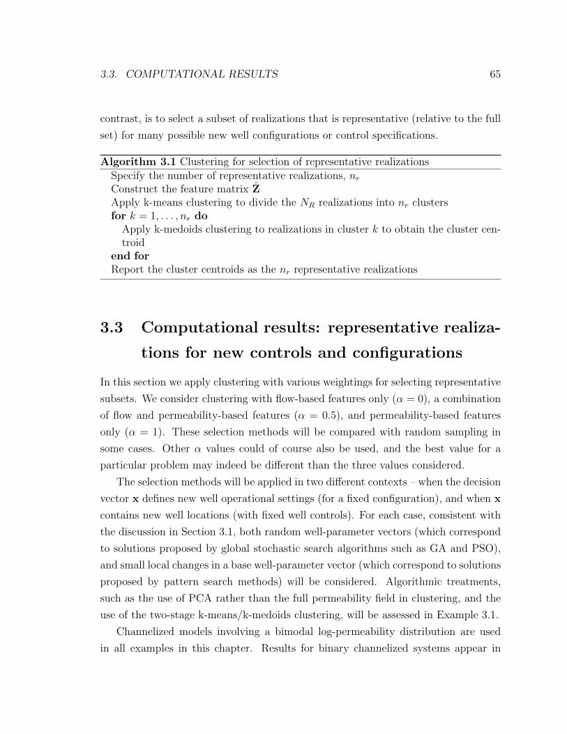
3.3. COMPUTATIONAL RESULTS 65
contrast, is to select a subset of realizations that is representative (relative to the full
set) for many possible new well configurations or control specifications.
Algorithm 3.1 Clustering for selection of representative realizations
Specify the number of representative realizations, nrConstruct the feature matrix ZApply k-means clustering to divide the NR realizations into nr clustersfor k = 1, . . . , nr do
Apply k-medoids clustering to realizations in cluster k to obtain the cluster cen-troid
end forReport the cluster centroids as the nr representative realizations
3.3 Computational results: representative realiza-
tions for new controls and configurations
In this section we apply clustering with various weightings for selecting representative
subsets. We consider clustering with flow-based features only (α = 0), a combination
of flow and permeability-based features (α = 0.5), and permeability-based features
only (α = 1). These selection methods will be compared with random sampling in
some cases. Other α values could of course also be used, and the best value for a
particular problem may indeed be different than the three values considered.
The selection methods will be applied in two different contexts – when the decision
vector x defines new well operational settings (for a fixed configuration), and when x
contains new well locations (with fixed well controls). For each case, consistent with
the discussion in Section 3.1, both random well-parameter vectors (which correspond
to solutions proposed by global stochastic search algorithms such as GA and PSO),
and small local changes in a base well-parameter vector (which correspond to solutions
proposed by pattern search methods) will be considered. Algorithmic treatments,
such as the use of PCA rather than the full permeability field in clustering, and the
use of the two-stage k-means/k-medoids clustering, will be assessed in Example 3.1.
Channelized models involving a bimodal log-permeability distribution are used
in all examples in this chapter. Results for binary channelized systems appear in
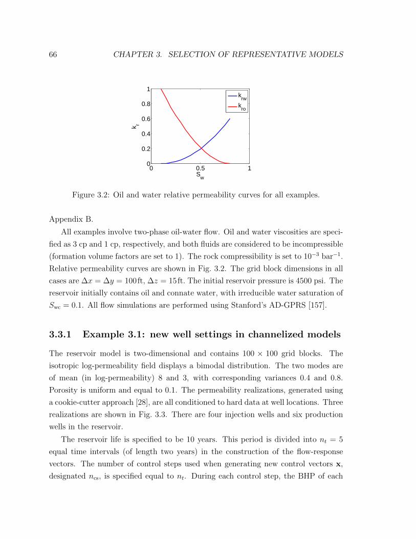
66 CHAPTER 3. SELECTION OF REPRESENTATIVE MODELS
0 0.5 10
0.2
0.4
0.6
0.8
1
Sw
k r
krw
kro
Figure 3.2: Oil and water relative permeability curves for all examples.
Appendix B.
All examples involve two-phase oil-water flow. Oil and water viscosities are speci-
fied as 3 cp and 1 cp, respectively, and both fluids are considered to be incompressible
(formation volume factors are set to 1). The rock compressibility is set to 10−3 bar−1.
Relative permeability curves are shown in Fig. 3.2. The grid block dimensions in all
cases are ∆x = ∆y = 100ft, ∆z = 15ft. The initial reservoir pressure is 4500 psi. The
reservoir initially contains oil and connate water, with irreducible water saturation of
Swc = 0.1. All flow simulations are performed using Stanford’s AD-GPRS [157].
3.3.1 Example 3.1: new well settings in channelized models
The reservoir model is two-dimensional and contains 100 × 100 grid blocks. The
isotropic log-permeability field displays a bimodal distribution. The two modes are
of mean (in log-permeability) 8 and 3, with corresponding variances 0.4 and 0.8.
Porosity is uniform and equal to 0.1. The permeability realizations, generated using
a cookie-cutter approach [28], are all conditioned to hard data at well locations. Three
realizations are shown in Fig. 3.3. There are four injection wells and six production
wells in the reservoir.
The reservoir life is specified to be 10 years. This period is divided into nt = 5
equal time intervals (of length two years) in the construction of the flow-response
vectors. The number of control steps used when generating new control vectors x,
designated ncs, is specified equal to nt. During each control step, the BHP of each
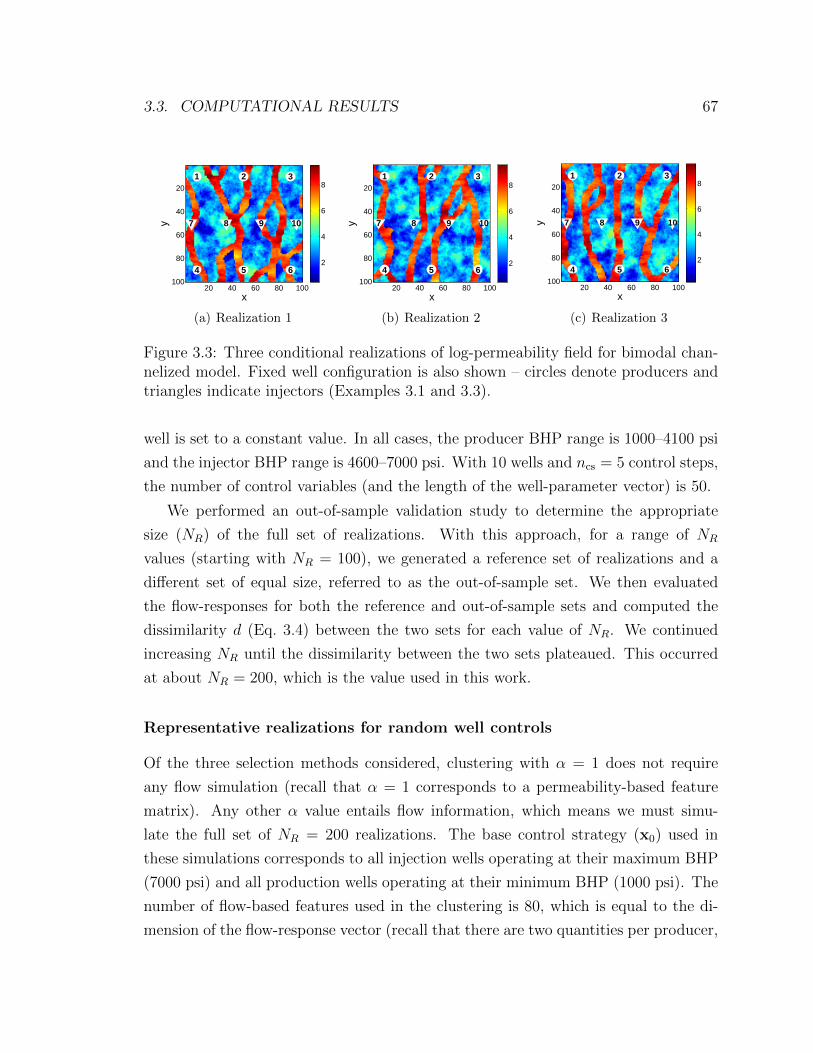
3.3. COMPUTATIONAL RESULTS 67
x
y
1 2 3
4 5 6
7 8 9 10
20 40 60 80 100
20
40
60
80
100
2
4
6
8
(a) Realization 1
x
y
1 2 3
4 5 6
7 8 9 10
20 40 60 80 100
20
40
60
80
100
2
4
6
8
(b) Realization 2
x
y
1 2 3
4 5 6
7 8 9 10
20 40 60 80 100
20
40
60
80
100
2
4
6
8
(c) Realization 3
Figure 3.3: Three conditional realizations of log-permeability field for bimodal chan-nelized model. Fixed well configuration is also shown – circles denote producers andtriangles indicate injectors (Examples 3.1 and 3.3).
well is set to a constant value. In all cases, the producer BHP range is 1000–4100 psi
and the injector BHP range is 4600–7000 psi. With 10 wells and ncs = 5 control steps,
the number of control variables (and the length of the well-parameter vector) is 50.
We performed an out-of-sample validation study to determine the appropriate
size (NR) of the full set of realizations. With this approach, for a range of NR
values (starting with NR = 100), we generated a reference set of realizations and a
different set of equal size, referred to as the out-of-sample set. We then evaluated
the flow-responses for both the reference and out-of-sample sets and computed the
dissimilarity d (Eq. 3.4) between the two sets for each value of NR. We continued
increasing NR until the dissimilarity between the two sets plateaued. This occurred
at about NR = 200, which is the value used in this work.
Representative realizations for random well controls
Of the three selection methods considered, clustering with α = 1 does not require
any flow simulation (recall that α = 1 corresponds to a permeability-based feature
matrix). Any other α value entails flow information, which means we must simu-
late the full set of NR = 200 realizations. The base control strategy (x0) used in
these simulations corresponds to all injection wells operating at their maximum BHP
(7000 psi) and all production wells operating at their minimum BHP (1000 psi). The
number of flow-based features used in the clustering is 80, which is equal to the di-
mension of the flow-response vector (recall that there are two quantities per producer,
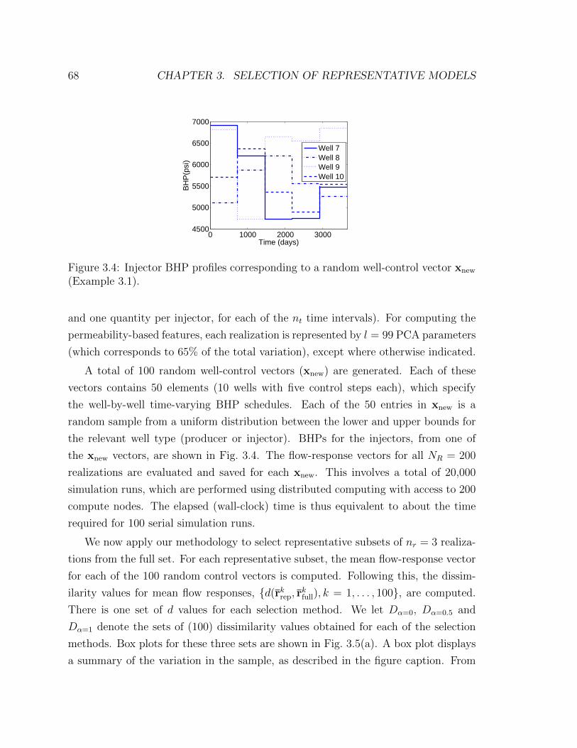
68 CHAPTER 3. SELECTION OF REPRESENTATIVE MODELS
0 1000 2000 30004500
5000
5500
6000
6500
7000
Time (days)
BH
P(p
si)
Well 7Well 8Well 9Well 10
Figure 3.4: Injector BHP profiles corresponding to a random well-control vector xnew
(Example 3.1).
and one quantity per injector, for each of the nt time intervals). For computing the
permeability-based features, each realization is represented by l = 99 PCA parameters
(which corresponds to 65% of the total variation), except where otherwise indicated.
A total of 100 random well-control vectors (xnew) are generated. Each of these
vectors contains 50 elements (10 wells with five control steps each), which specify
the well-by-well time-varying BHP schedules. Each of the 50 entries in xnew is a
random sample from a uniform distribution between the lower and upper bounds for
the relevant well type (producer or injector). BHPs for the injectors, from one of
the xnew vectors, are shown in Fig. 3.4. The flow-response vectors for all NR = 200
realizations are evaluated and saved for each xnew. This involves a total of 20,000
simulation runs, which are performed using distributed computing with access to 200
compute nodes. The elapsed (wall-clock) time is thus equivalent to about the time
required for 100 serial simulation runs.
We now apply our methodology to select representative subsets of nr = 3 realiza-
tions from the full set. For each representative subset, the mean flow-response vector
for each of the 100 random control vectors is computed. Following this, the dissim-
ilarity values for mean flow responses, {d(rkrep, rkfull), k = 1, . . . , 100}, are computed.
There is one set of d values for each selection method. We let Dα=0, Dα=0.5 and
Dα=1 denote the sets of (100) dissimilarity values obtained for each of the selection
methods. Box plots for these three sets are shown in Fig. 3.5(a). A box plot displays
a summary of the variation in the sample, as described in the figure caption. From
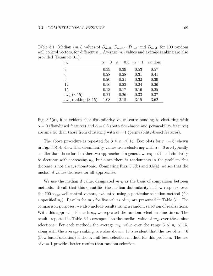
3.3. COMPUTATIONAL RESULTS 69
Table 3.1: Median (mD) values of Dα=0, Dα=0.5, Dα=1 and Drand, for 100 randomwell control vectors, for different nr. Average mD values and average ranking are alsoprovided (Example 3.1).
nr α = 0 α = 0.5 α = 1 random
3 0.39 0.39 0.53 0.576 0.28 0.28 0.31 0.419 0.20 0.21 0.32 0.3912 0.16 0.23 0.24 0.2615 0.13 0.17 0.16 0.25avg (3-15) 0.21 0.26 0.33 0.37avg ranking (3-15) 1.08 2.15 3.15 3.62
Fig. 3.5(a), it is evident that dissimilarity values corresponding to clustering with
α = 0 (flow-based features) and α = 0.5 (both flow-based and permeability features)
are smaller than those from clustering with α = 1 (permeability-based features).
The above procedure is repeated for 3 ≤ nr ≤ 15. Box plots for nr = 6, shown
in Fig. 3.5(b), show that dissimilarity values from clustering with α = 0 are typically
smaller than those for the other two approaches. In general we expect the dissimilarity
to decrease with increasing nr, but since there is randomness in the problem this
decrease is not always monotonic. Comparing Figs. 3.5(b) and 3.5(a), we see that the
median d values decrease for all approaches.
We use the median d value, designated mD, as the basis of comparison between
methods. Recall that this quantifies the median dissimilarity in flow response over
the 100 xnew well-control vectors, evaluated using a particular selection method (for
a specified nr). Results for mD for five values of nr are presented in Table 3.1. For
comparison purposes, we also include results using a random selection of realizations.
With this approach, for each nr, we repeated the random selection nine times. The
results reported in Table 3.1 correspond to the median value of mD over these nine
selections. For each method, the average mD value over the range 3 ≤ nr ≤ 15,
along with the average ranking, are also shown. It is evident that the use of α = 0
(flow-based selection) is the overall best selection method for this problem. The use
of α = 1 provides better results than random selection.

70 CHAPTER 3. SELECTION OF REPRESENTATIVE MODELS
0.35
0.4
0.45
0.5
0.55
α=0 α=0.5 α=1
D
(a) nr = 3
0.25
0.3
0.35
α=0 α=0.5 α=1
D
(b) nr = 6
Figure 3.5: Box plots of Dα=0, Dα=0.5 and Dα=1 for 100 random well control vectors.The red line within each box corresponds to the median, and the bottom and top ofeach box correspond to the 25th and 75th percentiles. The lines above and below theboxes correspond to the 2nd and 98th percentiles (Example 3.1).
As discussed in Section 3.2.1, flow-based features for clustering can also be gen-
erated from reduced-physics proxy simulations, and here we apply a tracer-type
constant-mobility proxy model (with krw = Sw, kro = 1− Sw, µw = µo). We perform
these proxy simulations for all realizations with the base control strategy to obtain
flow-based features for clustering. We then compute the flow-based distance ma-
trix (corresponding to α = 0), which is obtained by computing Euclidean distances
between feature vectors. With NR = 200, there are 19,900 distinct values in this
distance matrix. The correlation coefficient between these flow-based distances and
those computed from full-physics simulation was 0.8, which suggests the proxy flow
results should provide useful flow-based information in our procedure.
We let Dα,prx denote the set of dissimilarity (d) values obtained from realization
selection using proxy model flow features (here ‘prx’ designates proxy). Results for
median Dα,prx are presented in Table 3.2. Comparing these values to those for mD
using full-physics flow simulations (Table 3.1), we see that, on average, clustering
using proxy flow information performs nearly as well as clustering with full-physics
flow information for α = 0 (average mD of 0.23 versus 0.21), and equally well for
α = 0.5 (0.26 in both cases). Results are generally close for a particular nr value,
though some differences are apparent.
The average mD results for both α = 0 (prx) and α = 0.5 (prx) are clearly below
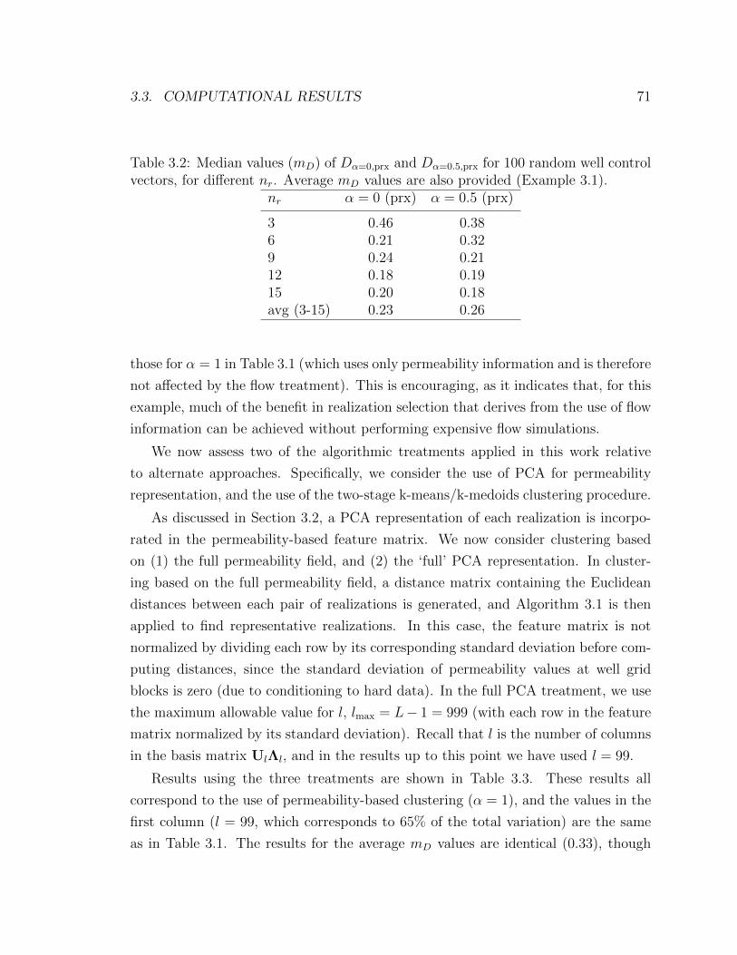
3.3. COMPUTATIONAL RESULTS 71
Table 3.2: Median values (mD) of Dα=0,prx and Dα=0.5,prx for 100 random well controlvectors, for different nr. Average mD values are also provided (Example 3.1).
nr α = 0 (prx) α = 0.5 (prx)
3 0.46 0.386 0.21 0.329 0.24 0.2112 0.18 0.1915 0.20 0.18avg (3-15) 0.23 0.26
those for α = 1 in Table 3.1 (which uses only permeability information and is therefore
not affected by the flow treatment). This is encouraging, as it indicates that, for this
example, much of the benefit in realization selection that derives from the use of flow
information can be achieved without performing expensive flow simulations.
We now assess two of the algorithmic treatments applied in this work relative
to alternate approaches. Specifically, we consider the use of PCA for permeability
representation, and the use of the two-stage k-means/k-medoids clustering procedure.
As discussed in Section 3.2, a PCA representation of each realization is incorpo-
rated in the permeability-based feature matrix. We now consider clustering based
on (1) the full permeability field, and (2) the ‘full’ PCA representation. In cluster-
ing based on the full permeability field, a distance matrix containing the Euclidean
distances between each pair of realizations is generated, and Algorithm 3.1 is then
applied to find representative realizations. In this case, the feature matrix is not
normalized by dividing each row by its corresponding standard deviation before com-
puting distances, since the standard deviation of permeability values at well grid
blocks is zero (due to conditioning to hard data). In the full PCA treatment, we use
the maximum allowable value for l, lmax = L− 1 = 999 (with each row in the feature
matrix normalized by its standard deviation). Recall that l is the number of columns
in the basis matrix UlΛl, and in the results up to this point we have used l = 99.
Results using the three treatments are shown in Table 3.3. These results all
correspond to the use of permeability-based clustering (α = 1), and the values in the
first column (l = 99, which corresponds to 65% of the total variation) are the same
as in Table 3.1. The results for the average mD values are identical (0.33), though
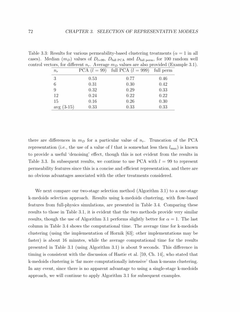
72 CHAPTER 3. SELECTION OF REPRESENTATIVE MODELS
Table 3.3: Results for various permeability-based clustering treatments (α = 1 in allcases). Median (mD) values of Dl=99, Dfull PCA and Dfull perm, for 100 random wellcontrol vectors, for different nr. Average mD values are also provided (Example 3.1).
nr PCA (l = 99) full PCA (l = 999) full perm
3 0.53 0.77 0.466 0.31 0.30 0.429 0.32 0.29 0.3312 0.24 0.22 0.2215 0.16 0.26 0.30avg (3-15) 0.33 0.33 0.33
there are differences in mD for a particular value of nr. Truncation of the PCA
representation (i.e., the use of a value of l that is somewhat less then lmax) is known
to provide a useful ‘denoising’ effect, though this is not evident from the results in
Table 3.3. In subsequent results, we continue to use PCA with l = 99 to represent
permeability features since this is a concise and efficient representation, and there are
no obvious advantages associated with the other treatments considered.
We next compare our two-stage selection method (Algorithm 3.1) to a one-stage
k-medoids selection approach. Results using k-medoids clustering, with flow-based
features from full-physics simulations, are presented in Table 3.4. Comparing these
results to those in Table 3.1, it is evident that the two methods provide very similar
results, though the use of Algorithm 3.1 performs slightly better for α = 1. The last
column in Table 3.4 shows the computational time. The average time for k-medoids
clustering (using the implementation of Hornik [63]; other implementations may be
faster) is about 16 minutes, while the average computational time for the results
presented in Table 3.1 (using Algorithm 3.1) is about 9 seconds. This difference in
timing is consistent with the discussion of Hastie et al. [59, Ch. 14], who stated that
k-medoids clustering is ‘far more computationally intensive’ than k-means clustering.
In any event, since there is no apparent advantage to using a single-stage k-medoids
approach, we will continue to apply Algorithm 3.1 for subsequent examples.
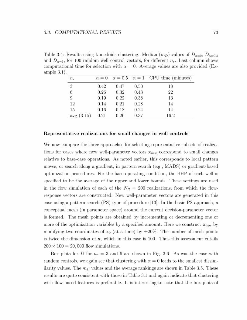
3.3. COMPUTATIONAL RESULTS 73
Table 3.4: Results using k-medoids clustering. Median (mD) values of Dα=0, Dα=0.5
and Dα=1, for 100 random well control vectors, for different nr. Last column showscomputational time for selection with α = 0. Average values are also provided (Ex-ample 3.1).
nr α = 0 α = 0.5 α = 1 CPU time (minutes)
3 0.42 0.47 0.50 186 0.26 0.32 0.43 229 0.19 0.22 0.38 1312 0.14 0.21 0.28 1415 0.16 0.18 0.24 14avg (3-15) 0.21 0.26 0.37 16.2
Representative realizations for small changes in well controls
We now compare the three approaches for selecting representative subsets of realiza-
tions for cases where new well-parameter vectors xnew correspond to small changes
relative to base-case operations. As noted earlier, this corresponds to local pattern
moves, or search along a gradient, in pattern search (e.g., MADS) or gradient-based
optimization procedures. For the base operating condition, the BHP of each well is
specified to be the average of the upper and lower bounds. These settings are used
in the flow simulation of each of the NR = 200 realizations, from which the flow-
response vectors are constructed. New well-parameter vectors are generated in this
case using a pattern search (PS) type of procedure [13]. In the basic PS approach, a
conceptual mesh (in parameter space) around the current decision-parameter vector
is formed. The mesh points are obtained by incrementing or decrementing one or
more of the optimization variables by a specified amount. Here we construct xnew by
modifying two coordinates of x0 (at a time) by ±20%. The number of mesh points
is twice the dimension of x, which in this case is 100. Thus this assessment entails
200× 100 = 20, 000 flow simulations.
Box plots for D for nr = 3 and 6 are shown in Fig. 3.6. As was the case with
random controls, we again see that clustering with α = 0 leads to the smallest dissim-
ilarity values. The mD values and the average rankings are shown in Table 3.5. These
results are quite consistent with those in Table 3.1 and again indicate that clustering
with flow-based features is preferable. It is interesting to note that the box plots of

74 CHAPTER 3. SELECTION OF REPRESENTATIVE MODELS
0.35
0.4
0.45
0.5
0.55
α=0 α=0.5 α=1
D
(a) nr = 3
0.26
0.27
0.28
0.29
0.3
0.31
0.32
α=0 α=0.5 α=1
D
(b) nr = 6
Figure 3.6: Box plots of Dα=0, Dα=0.5 and Dα=1 for 100 well control vectors corre-sponding to pattern search mesh points. The red line within each box correspondsto the median, and the bottom and top of each box correspond to the 25th and 75thpercentiles. The lines above and below the boxes correspond to the 2nd and 98thpercentiles (Example 3.1).
D in Fig. 3.6 span a narrower range than those in Fig. 3.5. This is because of the
smaller variation in the flow responses here than for the case with random controls.
Results using flow-based features obtained from proxy simulations are presented
in Table 3.6. These results are, on average, again comparable to those obtained from
selection using full-physics simulations (Table 3.5), indicating that proxy modeling
could be very useful in this setting.
3.3.2 Example 3.2: new well configurations
We now consider cases involving new well locations rather than new well controls.
This case is based on the same reservoir model as in Example 3.1 (Section 3.3.1).
However, since new well configurations are considered here, the realizations are not
conditioned to any hard data. In this example, well BHPs are held constant over the
run, with injector BHP equal to 7000 psi and producer BHP equal to 1000 psi. Three
realizations of the permeability field, along with three base well configurations, are
shown in Fig. 3.7. The simulation time frame is 10 years, which is divided into nt = 5
intervals for computing flow responses.

3.3. COMPUTATIONAL RESULTS 75
Table 3.5: Median (mD) values of Dα=0, Dα=0.5 and Dα=1, for 100 well control vectorscorresponding to pattern search mesh points, for different nr. Average mD values andaverage ranking are also provided (Example 3.1).
nr α = 0 α = 0.5 α = 1
3 0.36 0.41 0.536 0.26 0.28 0.329 0.22 0.16 0.2612 0.20 0.19 0.2415 0.13 0.16 0.24avg (3-15) 0.22 0.24 0.31avg ranking (3-15) 1.46 1.54 3.00
Table 3.6: Median values (mD) of Dα=0,prx and Dα=0.5,prx for 100 well control vectorscorresponding to pattern search mesh points, for different nr. Average mD values arealso provided (Example 3.1).
nr α = 0 (prx) α = 0.5 (prx)
3 0.33 0.276 0.30 0.269 0.32 0.2512 0.21 0.2515 0.13 0.15avg (3-15) 0.25 0.24
x
y
1 2 3
4 5 6
7 8 9 10
20 40 60 80 100
20
40
60
80
100
2
4
6
8
(a) x10
x
y
1
2
3
4
5
6
7
8
9
1020 40 60 80 100
20
40
60
80
100
2
4
6
8
(b) x20
x
y
1 2 3 4 5 6
7 8
9 10
20 40 60 80 100
20
40
60
80
100
2
4
6
8
(c) x30
Figure 3.7: Three realizations of log-permeability field and three base well configura-tions for computing flow-based features used in clustering. Circles denote producersand triangles indicate injectors (Example 3.2).
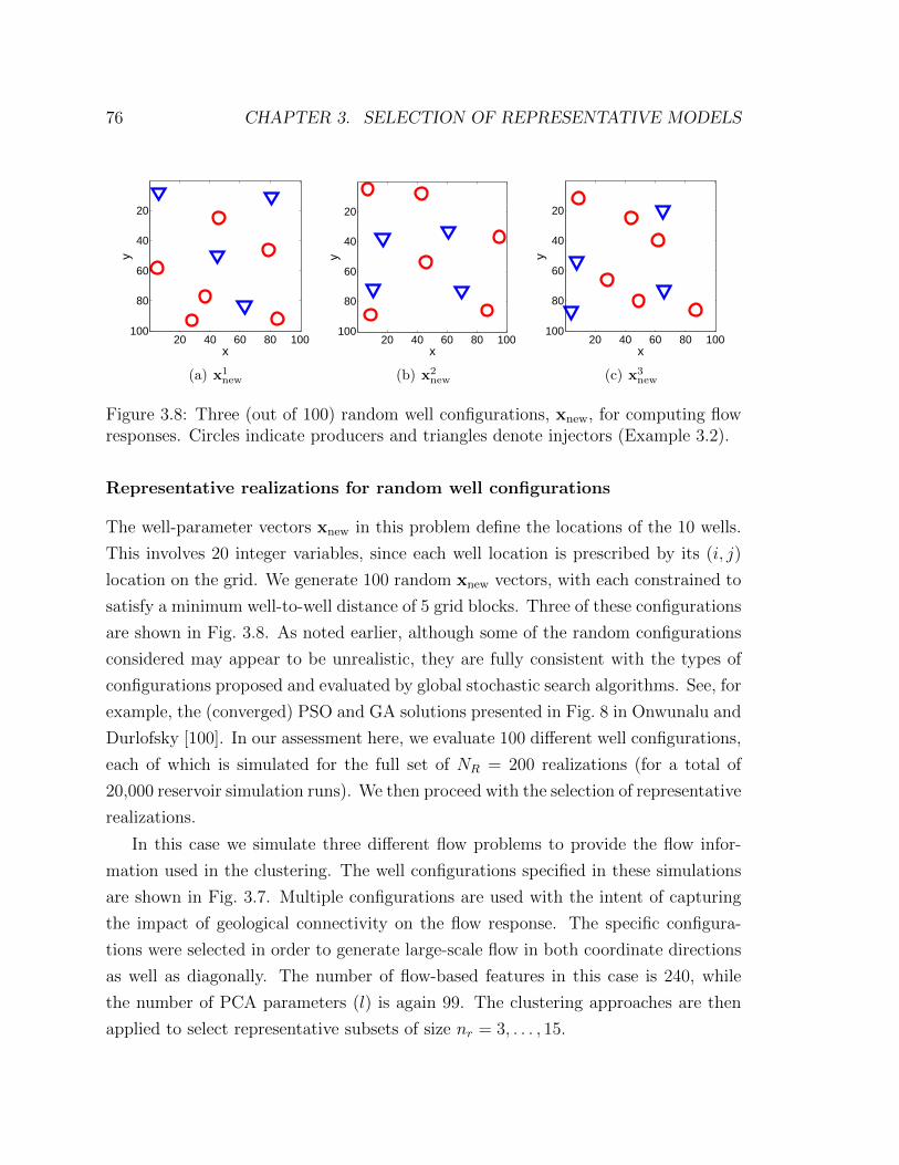
76 CHAPTER 3. SELECTION OF REPRESENTATIVE MODELS
x
y
20 40 60 80 100
20
40
60
80
100
(a) x1new
x
y20 40 60 80 100
20
40
60
80
100
(b) x2new
x
y
20 40 60 80 100
20
40
60
80
100
(c) x3new
Figure 3.8: Three (out of 100) random well configurations, xnew, for computing flowresponses. Circles indicate producers and triangles denote injectors (Example 3.2).
Representative realizations for random well configurations
The well-parameter vectors xnew in this problem define the locations of the 10 wells.
This involves 20 integer variables, since each well location is prescribed by its (i, j)
location on the grid. We generate 100 random xnew vectors, with each constrained to
satisfy a minimum well-to-well distance of 5 grid blocks. Three of these configurations
are shown in Fig. 3.8. As noted earlier, although some of the random configurations
considered may appear to be unrealistic, they are fully consistent with the types of
configurations proposed and evaluated by global stochastic search algorithms. See, for
example, the (converged) PSO and GA solutions presented in Fig. 8 in Onwunalu and
Durlofsky [100]. In our assessment here, we evaluate 100 different well configurations,
each of which is simulated for the full set of NR = 200 realizations (for a total of
20,000 reservoir simulation runs). We then proceed with the selection of representative
realizations.
In this case we simulate three different flow problems to provide the flow infor-
mation used in the clustering. The well configurations specified in these simulations
are shown in Fig. 3.7. Multiple configurations are used with the intent of capturing
the impact of geological connectivity on the flow response. The specific configura-
tions were selected in order to generate large-scale flow in both coordinate directions
as well as diagonally. The number of flow-based features in this case is 240, while
the number of PCA parameters (l) is again 99. The clustering approaches are then
applied to select representative subsets of size nr = 3, . . . , 15.
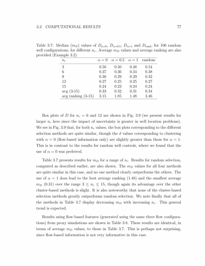
3.3. COMPUTATIONAL RESULTS 77
Table 3.7: Median (mD) values of Dα=0, Dα=0.5, Dα=1 and Drand, for 100 randomwell configurations, for different nr. Average mD values and average ranking are alsoprovided (Example 3.2).
nr α = 0 α = 0.5 α = 1 random
3 0.50 0.50 0.48 0.546 0.37 0.36 0.34 0.389 0.30 0.29 0.29 0.3212 0.27 0.25 0.25 0.2715 0.24 0.23 0.24 0.24avg (3-15) 0.33 0.32 0.31 0.34avg ranking (3-15) 3.15 1.85 1.48 3.46
Box plots of D for nr = 6 and 12 are shown in Fig. 3.9 (we present results for
larger nr here since the impact of uncertainty is greater in well location problems).
We see in Fig. 3.9 that, for both nr values, the box plots corresponding to the different
selection methods are quite similar, though the d values corresponding to clustering
with α = 0 (flow-based information only) are slightly greater than those for α = 1.
This is in contrast to the results for random well controls, where we found that the
use of α = 0 was preferred.
Table 3.7 presents results for mD for a range of nr. Results for random selection,
computed as described earlier, are also shown. The mD values for all four methods
are quite similar in this case, and no one method clearly outperforms the others. The
use of α = 1 does lead to the best average ranking (1.48) and the smallest average
mD (0.31) over the range 3 ≤ nr ≤ 15, though again its advantage over the other
cluster-based methods is slight. It is also noteworthy that none of the cluster-based
selection methods greatly outperforms random selection. We note finally that all of
the methods in Table 3.7 display decreasing mD with increasing nr. This general
trend is expected.
Results using flow-based features (generated using the same three flow configura-
tions) from proxy simulations are shown in Table 3.8. These results are identical, in
terms of average mD values, to those in Table 3.7. This is perhaps not surprising,
since flow-based information is not very informative in this case.
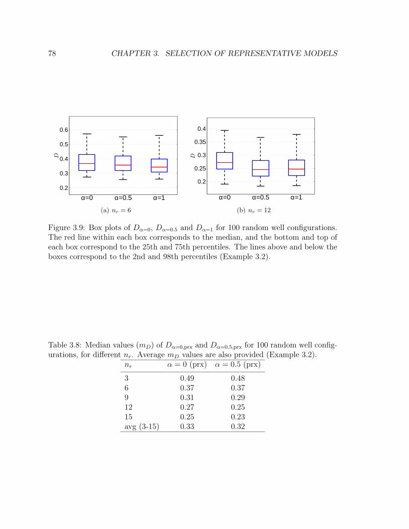
78 CHAPTER 3. SELECTION OF REPRESENTATIVE MODELS
0.2
0.3
0.4
0.5
0.6
α=0 α=0.5 α=1
D
(a) nr = 6
0.2
0.25
0.3
0.35
0.4
α=0 α=0.5 α=1D
(b) nr = 12
Figure 3.9: Box plots of Dα=0, Dα=0.5 and Dα=1 for 100 random well configurations.The red line within each box corresponds to the median, and the bottom and top ofeach box correspond to the 25th and 75th percentiles. The lines above and below theboxes correspond to the 2nd and 98th percentiles (Example 3.2).
Table 3.8: Median values (mD) of Dα=0,prx and Dα=0.5,prx for 100 random well config-urations, for different nr. Average mD values are also provided (Example 3.2).
nr α = 0 (prx) α = 0.5 (prx)
3 0.49 0.486 0.37 0.379 0.31 0.2912 0.27 0.2515 0.25 0.23avg (3-15) 0.33 0.32
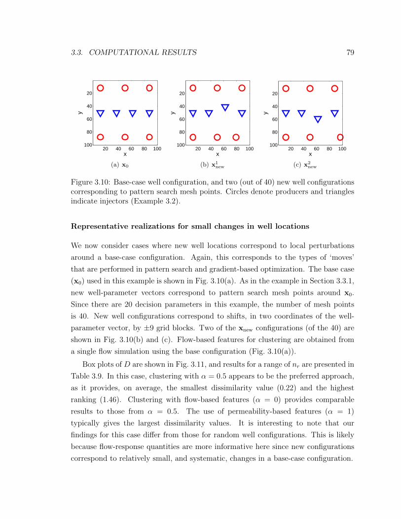
3.3. COMPUTATIONAL RESULTS 79
x
y
20 40 60 80 100
20
40
60
80
100
(a) x0
x
y
20 40 60 80 100
20
40
60
80
100
(b) x1new
x
y
20 40 60 80 100
20
40
60
80
100
(c) x2new
Figure 3.10: Base-case well configuration, and two (out of 40) new well configurationscorresponding to pattern search mesh points. Circles denote producers and trianglesindicate injectors (Example 3.2).
Representative realizations for small changes in well locations
We now consider cases where new well locations correspond to local perturbations
around a base-case configuration. Again, this corresponds to the types of ‘moves’
that are performed in pattern search and gradient-based optimization. The base case
(x0) used in this example is shown in Fig. 3.10(a). As in the example in Section 3.3.1,
new well-parameter vectors correspond to pattern search mesh points around x0.
Since there are 20 decision parameters in this example, the number of mesh points
is 40. New well configurations correspond to shifts, in two coordinates of the well-
parameter vector, by ±9 grid blocks. Two of the xnew configurations (of the 40) are
shown in Fig. 3.10(b) and (c). Flow-based features for clustering are obtained from
a single flow simulation using the base configuration (Fig. 3.10(a)).
Box plots of D are shown in Fig. 3.11, and results for a range of nr are presented in
Table 3.9. In this case, clustering with α = 0.5 appears to be the preferred approach,
as it provides, on average, the smallest dissimilarity value (0.22) and the highest
ranking (1.46). Clustering with flow-based features (α = 0) provides comparable
results to those from α = 0.5. The use of permeability-based features (α = 1)
typically gives the largest dissimilarity values. It is interesting to note that our
findings for this case differ from those for random well configurations. This is likely
because flow-response quantities are more informative here since new configurations
correspond to relatively small, and systematic, changes in a base-case configuration.
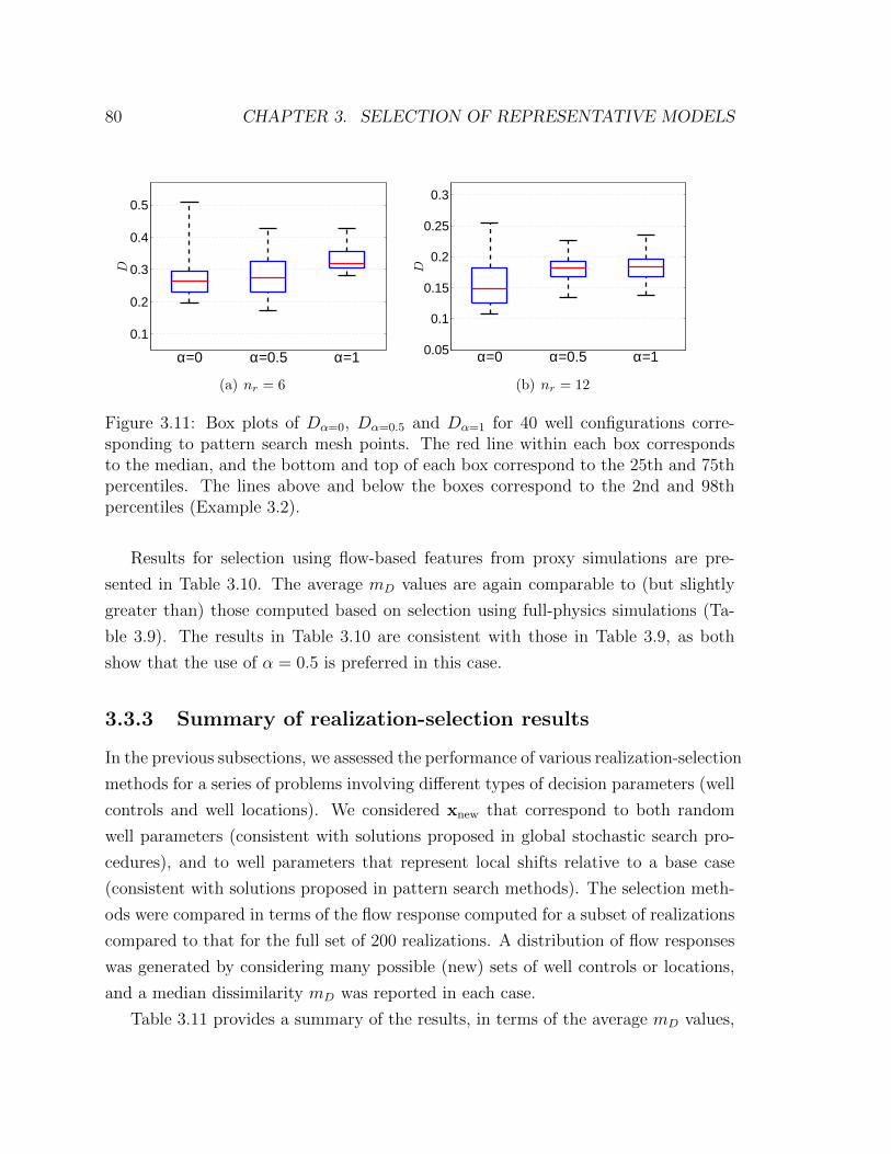
80 CHAPTER 3. SELECTION OF REPRESENTATIVE MODELS
0.1
0.2
0.3
0.4
0.5
α=0 α=0.5 α=1
D
(a) nr = 6
0.05
0.1
0.15
0.2
0.25
0.3
α=0 α=0.5 α=1
D
(b) nr = 12
Figure 3.11: Box plots of Dα=0, Dα=0.5 and Dα=1 for 40 well configurations corre-sponding to pattern search mesh points. The red line within each box correspondsto the median, and the bottom and top of each box correspond to the 25th and 75thpercentiles. The lines above and below the boxes correspond to the 2nd and 98thpercentiles (Example 3.2).
Results for selection using flow-based features from proxy simulations are pre-
sented in Table 3.10. The average mD values are again comparable to (but slightly
greater than) those computed based on selection using full-physics simulations (Ta-
ble 3.9). The results in Table 3.10 are consistent with those in Table 3.9, as both
show that the use of α = 0.5 is preferred in this case.
3.3.3 Summary of realization-selection results
In the previous subsections, we assessed the performance of various realization-selection
methods for a series of problems involving different types of decision parameters (well
controls and well locations). We considered xnew that correspond to both random
well parameters (consistent with solutions proposed in global stochastic search pro-
cedures), and to well parameters that represent local shifts relative to a base case
(consistent with solutions proposed in pattern search methods). The selection meth-
ods were compared in terms of the flow response computed for a subset of realizations
compared to that for the full set of 200 realizations. A distribution of flow responses
was generated by considering many possible (new) sets of well controls or locations,
and a median dissimilarity mD was reported in each case.
Table 3.11 provides a summary of the results, in terms of the average mD values,
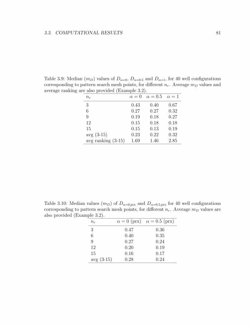
3.3. COMPUTATIONAL RESULTS 81
Table 3.9: Median (mD) values of Dα=0, Dα=0.5 and Dα=1, for 40 well configurationscorresponding to pattern search mesh points, for different nr. Average mD values andaverage ranking are also provided (Example 3.2).
nr α = 0 α = 0.5 α = 1
3 0.43 0.40 0.676 0.27 0.27 0.329 0.19 0.18 0.2712 0.15 0.18 0.1815 0.15 0.13 0.19avg (3-15) 0.23 0.22 0.32avg ranking (3-15) 1.69 1.46 2.85
Table 3.10: Median values (mD) of Dα=0,prx and Dα=0.5,prx for 40 well configurationscorresponding to pattern search mesh points, for different nr. Average mD values arealso provided (Example 3.2).
nr α = 0 (prx) α = 0.5 (prx)
3 0.47 0.366 0.40 0.359 0.27 0.2412 0.20 0.1915 0.16 0.17avg (3-15) 0.28 0.24
82 CHAPTER 3. SELECTION OF REPRESENTATIVE MODELS
for the four cases considered in this chapter. Results for α = 0 and α = 0.5 are
provided for selection using both full-physics and proxy simulations. For the cases
involving new well controls (either random or pattern search shifts relative to the base
case), the best performing method for selecting a representative subset was clustering
with flow-based features (α = 0). For randomly-generated new well configurations,
the three selection methods performed similarly, though selection with permeability-
based features (α = 1) provided slightly better results than the other approaches.
Finally, for small well-location changes relative to a base well configuration, realiza-
tions selected using α = 0.5 provided the best results. The results for binary systems
presented in Appendix B are generally consistent with the results in Table 3.11.
The use of tracer-type constant-mobility (proxy) simulations to obtain flow-based
features for clustering appears to be quite suitable for the cases considered here, as
it provides results of nearly the quality of those using full-physics simulations. It
would be expected, however, that this particular proxy model will be less effective for
cases with more challenging flow physics; i.e., systems with strong compressibility or
three-phase flow effects, or those involving complex recovery processes such as steam
injection. For such cases, alternative proxies could presumably be developed, though
this would require some amount of numerical experimentation.
Taken in total, these results demonstrate the benefit of using base-case flow infor-
mation for the selection of representative realizations in many situations. Flow data
are quite informative when well controls are varied, which seems reasonable since one
would expect that, with fixed well locations, the impact of geology for a particular
realization can be estimated from the base-case simulation. Flow information was
also found to be useful for selecting realizations in cases when the new well configu-
rations correspond to systematic (local) perturbations around the base case. This is
again reasonable as the base-case flow data in such situations are also expected to be
relevant to the new simulations. In general, however, for a particular system and set
of optimization parameters or decisions, some amount of numerical experimentation
may be required to determine the optimal value of α.
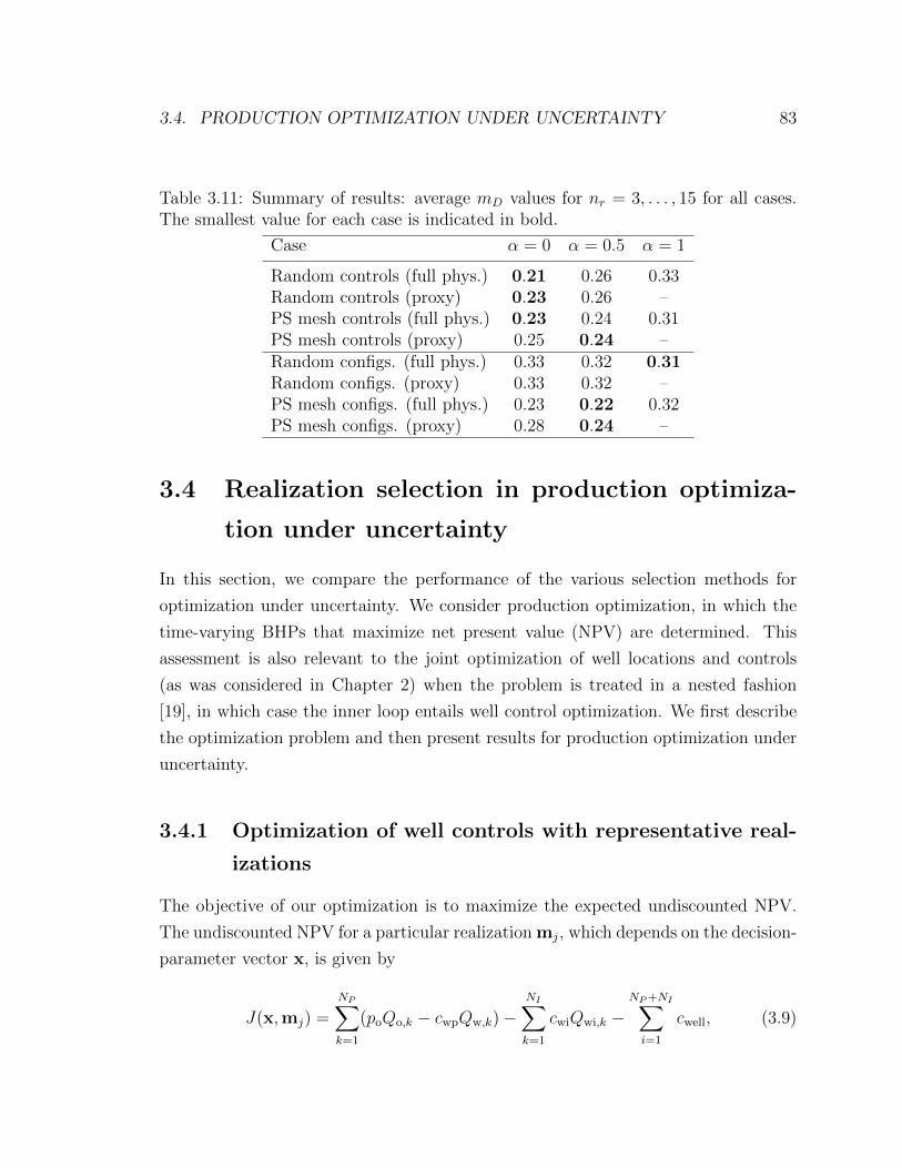
3.4. PRODUCTION OPTIMIZATION UNDER UNCERTAINTY 83
Table 3.11: Summary of results: average mD values for nr = 3, . . . , 15 for all cases.The smallest value for each case is indicated in bold.
Case α = 0 α = 0.5 α = 1
Random controls (full phys.) 0.21 0.26 0.33Random controls (proxy) 0.23 0.26 –PS mesh controls (full phys.) 0.23 0.24 0.31PS mesh controls (proxy) 0.25 0.24 –Random configs. (full phys.) 0.33 0.32 0.31Random configs. (proxy) 0.33 0.32 –PS mesh configs. (full phys.) 0.23 0.22 0.32PS mesh configs. (proxy) 0.28 0.24 –
3.4 Realization selection in production optimiza-
tion under uncertainty
In this section, we compare the performance of the various selection methods for
optimization under uncertainty. We consider production optimization, in which the
time-varying BHPs that maximize net present value (NPV) are determined. This
assessment is also relevant to the joint optimization of well locations and controls
(as was considered in Chapter 2) when the problem is treated in a nested fashion
[19], in which case the inner loop entails well control optimization. We first describe
the optimization problem and then present results for production optimization under
uncertainty.
3.4.1 Optimization of well controls with representative real-
izations
The objective of our optimization is to maximize the expected undiscounted NPV.
The undiscounted NPV for a particular realization mj, which depends on the decision-
parameter vector x, is given by
J(x,mj) =
NP∑k=1
(poQo,k − cwpQw,k)−NI∑k=1
cwiQwi,k −NP+NI∑i=1
cwell, (3.9)
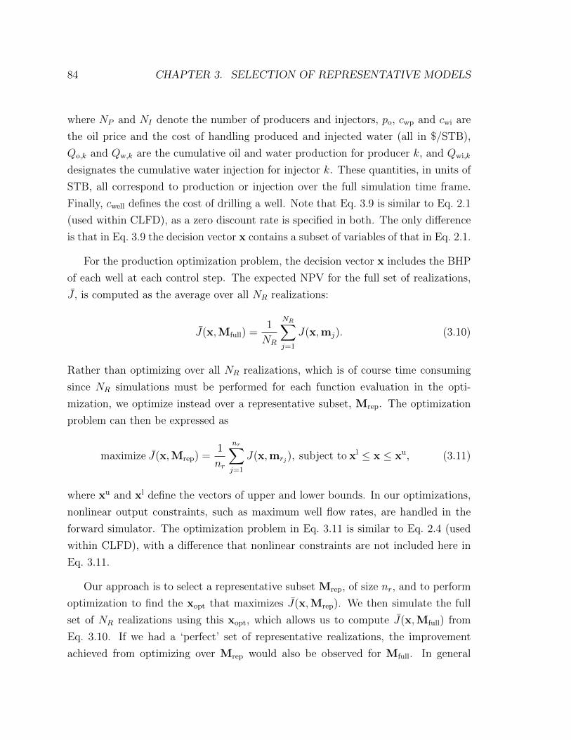
84 CHAPTER 3. SELECTION OF REPRESENTATIVE MODELS
where NP and NI denote the number of producers and injectors, po, cwp and cwi are
the oil price and the cost of handling produced and injected water (all in $/STB),
Qo,k and Qw,k are the cumulative oil and water production for producer k, and Qwi,k
designates the cumulative water injection for injector k. These quantities, in units of
STB, all correspond to production or injection over the full simulation time frame.
Finally, cwell defines the cost of drilling a well. Note that Eq. 3.9 is similar to Eq. 2.1
(used within CLFD), as a zero discount rate is specified in both. The only difference
is that in Eq. 3.9 the decision vector x contains a subset of variables of that in Eq. 2.1.
For the production optimization problem, the decision vector x includes the BHP
of each well at each control step. The expected NPV for the full set of realizations,
J , is computed as the average over all NR realizations:
J(x,Mfull) =1
NR
NR∑j=1
J(x,mj). (3.10)
Rather than optimizing over all NR realizations, which is of course time consuming
since NR simulations must be performed for each function evaluation in the opti-
mization, we optimize instead over a representative subset, Mrep. The optimization
problem can then be expressed as
maximize J(x,Mrep) =1
nr
nr∑j=1
J(x,mrj), subject to xl ≤ x ≤ xu, (3.11)
where xu and xl define the vectors of upper and lower bounds. In our optimizations,
nonlinear output constraints, such as maximum well flow rates, are handled in the
forward simulator. The optimization problem in Eq. 3.11 is similar to Eq. 2.4 (used
within CLFD), with a difference that nonlinear constraints are not included here in
Eq. 3.11.
Our approach is to select a representative subset Mrep, of size nr, and to perform
optimization to find the xopt that maximizes J(x,Mrep). We then simulate the full
set of NR realizations using this xopt, which allows us to compute J(x,Mfull) from
Eq. 3.10. If we had a ‘perfect’ set of representative realizations, the improvement
achieved from optimizing over Mrep would also be observed for Mfull. In general
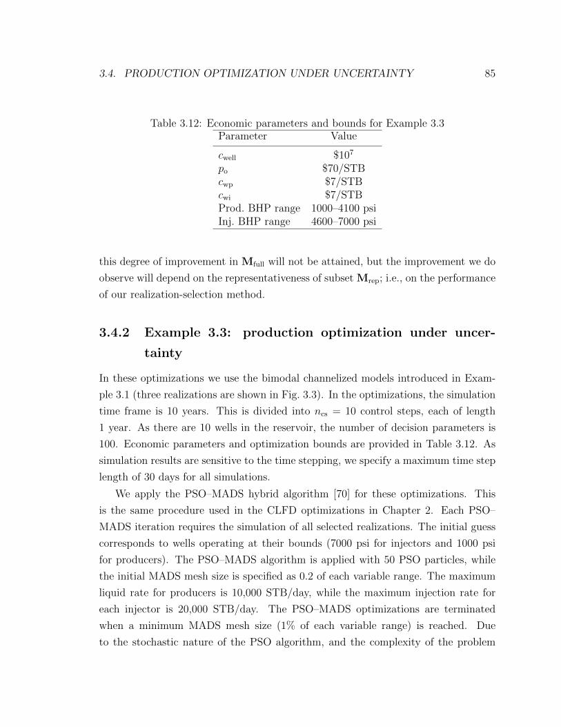
3.4. PRODUCTION OPTIMIZATION UNDER UNCERTAINTY 85
Table 3.12: Economic parameters and bounds for Example 3.3Parameter Value
cwell $107
po $70/STBcwp $7/STBcwi $7/STBProd. BHP range 1000–4100 psiInj. BHP range 4600–7000 psi
this degree of improvement in Mfull will not be attained, but the improvement we do
observe will depend on the representativeness of subset Mrep; i.e., on the performance
of our realization-selection method.
3.4.2 Example 3.3: production optimization under uncer-
tainty
In these optimizations we use the bimodal channelized models introduced in Exam-
ple 3.1 (three realizations are shown in Fig. 3.3). In the optimizations, the simulation
time frame is 10 years. This is divided into ncs = 10 control steps, each of length
1 year. As there are 10 wells in the reservoir, the number of decision parameters is
100. Economic parameters and optimization bounds are provided in Table 3.12. As
simulation results are sensitive to the time stepping, we specify a maximum time step
length of 30 days for all simulations.
We apply the PSO–MADS hybrid algorithm [70] for these optimizations. This
is the same procedure used in the CLFD optimizations in Chapter 2. Each PSO–
MADS iteration requires the simulation of all selected realizations. The initial guess
corresponds to wells operating at their bounds (7000 psi for injectors and 1000 psi
for producers). The PSO–MADS algorithm is applied with 50 PSO particles, while
the initial MADS mesh size is specified as 0.2 of each variable range. The maximum
liquid rate for producers is 10,000 STB/day, while the maximum injection rate for
each injector is 20,000 STB/day. The PSO–MADS optimizations are terminated
when a minimum MADS mesh size (1% of each variable range) is reached. Due
to the stochastic nature of the PSO algorithm, and the complexity of the problem
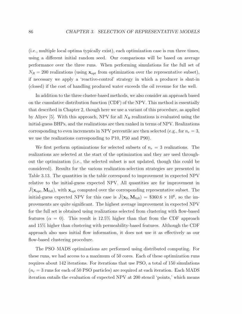
86 CHAPTER 3. SELECTION OF REPRESENTATIVE MODELS
(i.e., multiple local optima typically exist), each optimization case is run three times,
using a different initial random seed. Our comparisons will be based on average
performance over the three runs. When performing simulations for the full set of
NR = 200 realizations (using xopt from optimization over the representative subset),
if necessary we apply a ‘reactive-control’ strategy in which a producer is shut-in
(closed) if the cost of handling produced water exceeds the oil revenue for the well.
In addition to the three cluster-based methods, we also consider an approach based
on the cumulative distribution function (CDF) of the NPV. This method is essentially
that described in Chapter 2, though here we use a variant of this procedure, as applied
by Aliyev [5]. With this approach, NPV for all NR realizations is evaluated using the
initial-guess BHPs, and the realizations are then ranked in terms of NPV. Realizations
corresponding to even increments in NPV percentile are then selected (e.g., for nr = 3,
we use the realizations corresponding to P10, P50 and P90).
We first perform optimizations for selected subsets of nr = 3 realizations. The
realizations are selected at the start of the optimization and they are used through-
out the optimization (i.e., the selected subset is not updated, though this could be
considered). Results for the various realization-selection strategies are presented in
Table 3.13. The quantities in the table correspond to improvement in expected NPV
relative to the initial-guess expected NPV. All quantities are for improvement in
J(xopt,Mfull), with xopt computed over the corresponding representative subset. The
initial-guess expected NPV for this case is J(x0,Mfull) = $360.6 × 10⁶, so the im-
provements are quite significant. The highest average improvement in expected NPV
for the full set is obtained using realizations selected from clustering with flow-based
features (α = 0). This result is 12.5% higher than that from the CDF approach
and 15% higher than clustering with permeability-based features. Although the CDF
approach also uses initial flow information, it does not use it as effectively as our
flow-based clustering procedure.
The PSO–MADS optimizations are performed using distributed computing. For
these runs, we had access to a maximum of 50 cores. Each of these optimization runs
requires about 142 iterations. For iterations that use PSO, a total of 150 simulations
(nr = 3 runs for each of 50 PSO particles) are required at each iteration. Each MADS
iteration entails the evaluation of expected NPV at 200 stencil ‘points,’ which means
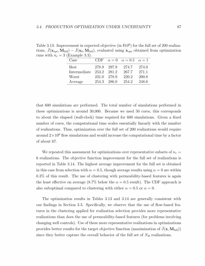
3.4. PRODUCTION OPTIMIZATION UNDER UNCERTAINTY 87
Table 3.13: Improvement in expected objective (in $106) for the full set of 200 realiza-tions, J(xopt,Mfull) − J(x0,Mfull), evaluated using xopt obtained from optimizationruns with nr = 3 (Example 3.3).
Case CDF α = 0 α = 0.5 α = 1
Best 278.9 297.9 274.7 274.0Intermediate 253.2 281.2 267.7 271.1Worst 231.0 278.9 220.2 200.8Average 254.3 286.0 254.2 248.6
that 600 simulations are performed. The total number of simulations performed in
these optimizations is around 30,000. Because we used 50 cores, this corresponds
to about the elapsed (wall-clock) time required for 600 simulations. Given a fixed
number of cores, the computational time scales essentially linearly with the number
of realizations. Thus, optimization over the full set of 200 realizations would require
around 2×10⁶ flow simulations and would increase the computational time by a factor
of about 67.
We repeated this assessment for optimizations over representative subsets of nr =
6 realizations. The objective function improvement for the full set of realizations is
reported in Table 3.14. The highest average improvement for the full set is obtained
in this case from selection with α = 0.5, though average results using α = 0 are within
0.3% of this result. The use of clustering with permeability-based features is again
the least effective on average (8.7% below the α = 0.5 result). The CDF approach is
also suboptimal compared to clustering with either α = 0.5 or α = 0.
The optimization results in Tables 3.13 and 3.14 are generally consistent with
our findings in Section 3.3. Specifically, we observe that the use of flow-based fea-
tures in the clustering applied for realization selection provides more representative
realizations than does the use of permeability-based features (for problems involving
changing well controls). Use of these more representative realizations in optimizations
provides better results for the target objective function (maximization of J(x,Mfull))
since they better capture the overall behavior of the full set of NR realizations.
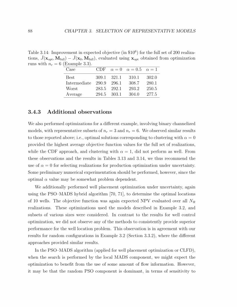
88 CHAPTER 3. SELECTION OF REPRESENTATIVE MODELS
Table 3.14: Improvement in expected objective (in $106) for the full set of 200 realiza-tions, J(xopt,Mfull) − J(x0,Mfull), evaluated using xopt obtained from optimizationruns with nr = 6 (Example 3.3).
Case CDF α = 0 α = 0.5 α = 1
Best 309.1 321.1 310.1 302.0Intermediate 290.9 296.1 308.7 280.1Worst 283.5 292.1 293.2 250.5Average 294.5 303.1 304.0 277.5
3.4.3 Additional observations
We also performed optimizations for a different example, involving binary channelized
models, with representative subsets of nr = 3 and nr = 6. We observed similar results
to those reported above; i.e., optimal solutions corresponding to clustering with α = 0
provided the highest average objective function values for the full set of realizations,
while the CDF approach, and clustering with α = 1, did not perform as well. From
these observations and the results in Tables 3.13 and 3.14, we thus recommend the
use of α = 0 for selecting realizations for production optimization under uncertainty.
Some preliminary numerical experimentation should be performed, however, since the
optimal α value may be somewhat problem dependent.
We additionally performed well placement optimization under uncertainty, again
using the PSO–MADS hybrid algorithm [70, 71], to determine the optimal locations
of 10 wells. The objective function was again expected NPV evaluated over all NR
realizations. These optimizations used the models described in Example 3.2, and
subsets of various sizes were considered. In contrast to the results for well control
optimization, we did not observe any of the methods to consistently provide superior
performance for the well location problem. This observation is in agreement with our
results for random configurations in Example 3.2 (Section 3.3.2), where the different
approaches provided similar results.
In the PSO–MADS algorithm (applied for well placement optimization or CLFD),
when the search is performed by the local MADS component, we might expect the
optimization to benefit from the use of some amount of flow information. However,
it may be that the random PSO component is dominant, in terms of sensitivity to
3.4. PRODUCTION OPTIMIZATION UNDER UNCERTAINTY 89
selected realizations, and the overall results reflect this. It is thus possible that an
adaptive-selection procedure, where the subset of realizations is updated during the
course of the optimization, might be beneficial. In such an approach, at early iter-
ations (when the search is dominated by PSO), representative realizations would be
selected using α = 1. At later (MADS-dominated) iterations, however, realizations
would be reselected using flow-based features (α = 0 or α = 0.5). Such an ap-
proach, which should be developed in future work, will require the determination of
appropriate ‘switching’ criteria and α values. This will require detailed investigation
since these quantities may depend on nr, the progress of the optimization, and other
parameters.
3.4.4 Summary
In this chapter, we developed a general method, based on clustering, to select a
representative subset of geological realizations from a large set. Prior to clustering,
each geological realization is represented by a feature vector composed of flow-based
and permeability-based quantities, weighted by a specified α factor. The use of both
full-physics and proxy-type tracer flow information was investigated in this setting.
We introduced and applied a statistical approach for comparing various selection
methods for a range of problems involving new well controls and new well locations,
generated either randomly or by small changes around a base case.
Based on our overall findings in this chapter, we recommend the use of flow-based
clustering (α = 0, using full-physics simulations if feasible) for optimizations involv-
ing well controls, and α = 0.5 for (local) pattern-search-based optimization of well
configurations. For optimization of well locations using a stochastic search procedure
(e.g., PSO or GA), the realization-selection methods are expected to perform compa-
rably. In this case permeability-based clustering is preferable since it does not require
any additional flow simulations. When practical, however, numerical experimentation
along the lines of the assessments presented in this chapter should be performed to
determine the appropriate value of α for the particular problem of interest. The com-
putational cost of such experimentation will often be reasonable, especially if proxy
flow information is used, compared to the cost associated with optimization under
geological uncertainty.

90 CHAPTER 3. SELECTION OF REPRESENTATIVE MODELS
Chapter 4
Optimization of Economic Project
Life for Reservoir Operations
In the optimizations presented in Chapters 2 and 3, we specified the project life
and then optimized NPV. Project life here refers to the timeframe in which the
reservoir operates with the existing wells – actual reservoir life may be extended by
drilling new wells. This type of specification is the usual approach taken in reservoir
optimization problems. In this chapter we consider a much more detailed treatment
of reservoir economics that entails the optimization of economic project life along
with the optimization of well controls.
In particular, we present a new formulation for the joint optimization of economic
project life (EPL) and well controls. This formulation includes the specification of a
a minimum attractive rate of return (MARR or hurdle rate) for the project. After
formulating the joint optimization problem in a nested fashion, we present an iterative
procedure that involves driving the rate of return (which varies with project life) to the
specified MARR, while maximizing NPV. The problem specification and the results
we present should be useful in practical settings because they enable the operator
to plan for infill drilling or redevelopment operations to avoid situations where NPV
increases slowly in time, but the benefit relative to the capital employed is extremely
low.
In the next section, we present our approach for the computation of the rate of
91
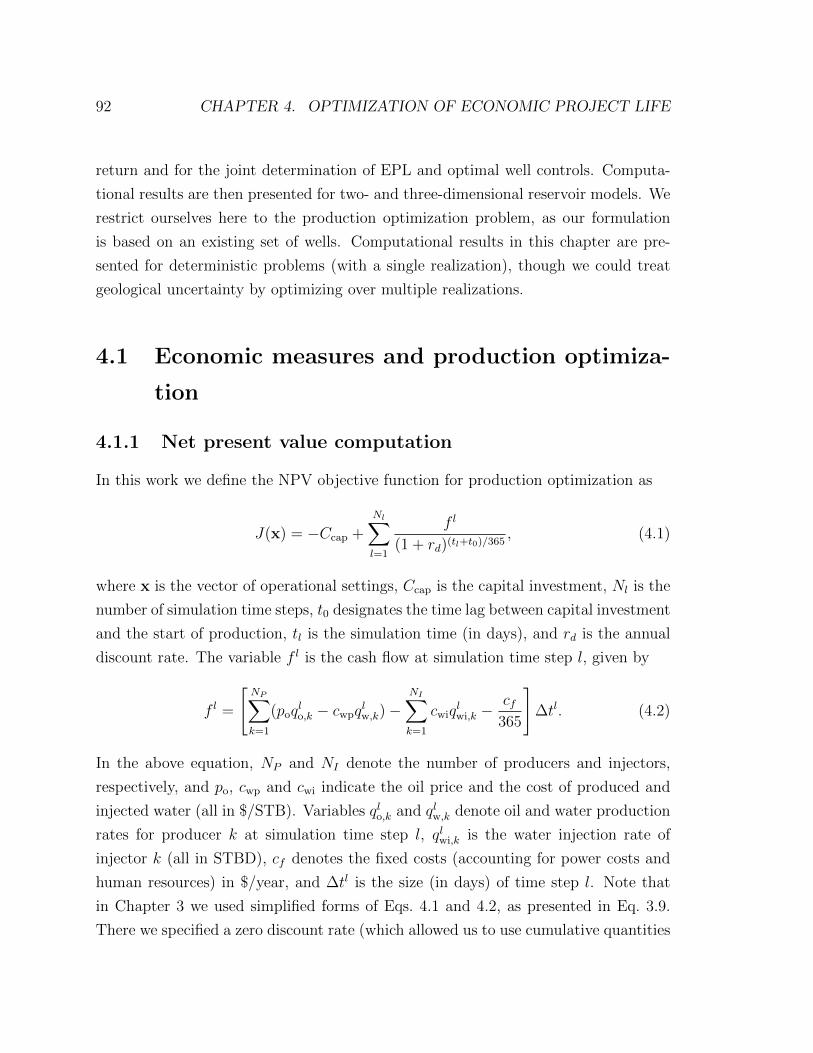
92 CHAPTER 4. OPTIMIZATION OF ECONOMIC PROJECT LIFE
return and for the joint determination of EPL and optimal well controls. Computa-
tional results are then presented for two- and three-dimensional reservoir models. We
restrict ourselves here to the production optimization problem, as our formulation
is based on an existing set of wells. Computational results in this chapter are pre-
sented for deterministic problems (with a single realization), though we could treat
geological uncertainty by optimizing over multiple realizations.
4.1 Economic measures and production optimiza-
tion
4.1.1 Net present value computation
In this work we define the NPV objective function for production optimization as
J(x) = −Ccap +
Nl∑l=1
f l
(1 + rd)(tl+t0)/365, (4.1)
where x is the vector of operational settings, Ccap is the capital investment, Nl is the
number of simulation time steps, t0 designates the time lag between capital investment
and the start of production, tl is the simulation time (in days), and rd is the annual
discount rate. The variable f l is the cash flow at simulation time step l, given by
f l =
[NP∑k=1
(poqlo,k − cwpq
lw,k)−
NI∑k=1
cwiqlwi,k −
cf365
]∆tl. (4.2)
In the above equation, NP and NI denote the number of producers and injectors,
respectively, and po, cwp and cwi indicate the oil price and the cost of produced and
injected water (all in $/STB). Variables qlo,k and qlw,k denote oil and water production
rates for producer k at simulation time step l, qlwi,k is the water injection rate of
injector k (all in STBD), cf denotes the fixed costs (accounting for power costs and
human resources) in $/year, and ∆tl is the size (in days) of time step l. Note that
in Chapter 3 we used simplified forms of Eqs. 4.1 and 4.2, as presented in Eq. 3.9.
There we specified a zero discount rate (which allowed us to use cumulative quantities

4.1. ECONOMIC MEASURES AND PRODUCTION OPTIMIZATION 93
instead of production/injection rates at each time step) and zero fixed cost.
The variable x is the vector of decision parameters that specify the operational
settings (here we control BHP) of all wells. In the problem formulation, the project
life is divided into ncs equal intervals, where each interval defines a control step.
4.1.2 Modified internal rate of return and economic project
life
We now describe the computation of the rate of return. As discussed in Chapter 1,
there are various ways of computing this quantity. These include the internal rate
of return (IRR), modified internal rate of return (MIRR) [88], and average internal
rate of return (AIRR) [91]. Among these measures, we have found MIRR to be the
most suitable for determining economic project lifetime in the context of production
optimization. This is because MIRR accounts for capital value and it is sensitive
to project timeframe. IRR, by contrast, is not sensitive to project lifetime, while
computing AIRR requires the specification of the capital value of the project at each
control step, which involves the introduction of additional assumptions.
MIRR is defined as the discount rate at which the future value of return is equal to
the present value of investment. Computation of MIRR requires the specification of
a reinvestment rate, which is the interest rate applied when reinvesting intermediate
positive cash flows. The positive cash flows are then compounded to the end of the
project life, while the negative cash flows are discounted to time zero. This reduces
the sequence of time-varying cash flows to two key values, an equivalent initial cost
or “present value of investment” (designated Cp) and a final income or “future value
of return” (denoted by Rf). In this work, we assume that the reinvestment rate is
equal to the discount rate, i.e., funds are borrowed and reinvested at the same rate.
This assumption is consistent with the NPV computation, which applies the same
discount rate to positive and negative cash flows (see, e.g., Shull [116], Balyeat et al.
[14]). Depending on the specific project circumstances, however, different values could
be specified for the discount and reinvestment rates. We now describe the detailed
computation of MIRR.
The cash flow values in Eq. 4.1 are computed at every simulation time step.
Because time steps vary, it is more convenient to compute MIRR based on control

94 CHAPTER 4. OPTIMIZATION OF ECONOMIC PROJECT LIFE
steps, which are of equal duration in our formulation. We let F ics designate the cash
flow for control step i, computed as
F ics =
∑l, ti−1<tl≤ti
f l. (4.3)
Here ti (= i∆tcs) is the end time for control step i, where control step i = 1, . . . , ncs
corresponds to the period (ti−1, ti), and ∆tcs is the length of each control step (for
i = 1, the control period is (0, t1)). After computing the cash flow for each control
step, we proceed with the computation of Cp and Rf. The present value of investment
(Cp) accounts for the capital investment and negative cash flows, i.e.,
Cp = Ccap +ncs∑
i,F ics<0
F ics(1 + rd)
−(ti+t0)/365, (4.4)
where the summation only includes negative cash flows (if any exist). The future
value of return, Rf, is expressed as
Rf =ncs∑
i,F ics>0
F ics(1 + rd)
(T−ti)/365, (4.5)
which only includes positive cash flows. Here T is the final simulation time (in days).
An example of a cash flow stream in a reservoir optimization problem is shown in
Fig. 4.1. This case corresponds to Example 4.1 below with rd = 0.05, t0 = 180 days,
T = 3240 days, and an initial investment of $360 MM. Cash flows are computed
every 90 days after the start of production. There are no negative cash flows so we
have Cp = $360 MM. Computing Rf, however, involves compounding all positive cash
flows to the end of project timeframe.
As stated earlier, MIRR, designated im, is the discount rate for which the future
value of return, Rf, becomes equal to the present value of investment, Cp. After
computing Rf and Cp, im is obtained from solving
Cp =Rf
(1 + im)(T+t0)/365. (4.6)
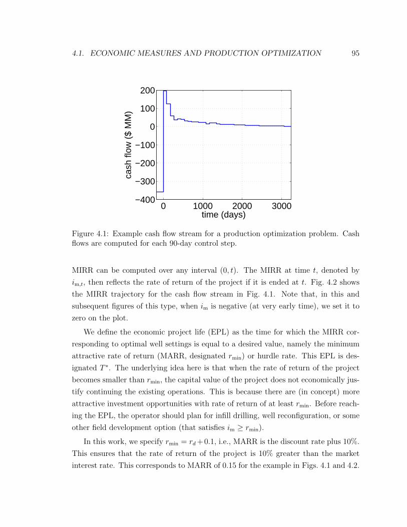
4.1. ECONOMIC MEASURES AND PRODUCTION OPTIMIZATION 95
0 1000 2000 3000−400
−300
−200
−100
0
100
200
time (days)
cash
flow
($
MM
)
Figure 4.1: Example cash flow stream for a production optimization problem. Cashflows are computed for each 90-day control step.
MIRR can be computed over any interval (0, t). The MIRR at time t, denoted by
im,t, then reflects the rate of return of the project if it is ended at t. Fig. 4.2 shows
the MIRR trajectory for the cash flow stream in Fig. 4.1. Note that, in this and
subsequent figures of this type, when im is negative (at very early time), we set it to
zero on the plot.
We define the economic project life (EPL) as the time for which the MIRR cor-
responding to optimal well settings is equal to a desired value, namely the minimum
attractive rate of return (MARR, designated rmin) or hurdle rate. This EPL is des-
ignated T ∗. The underlying idea here is that when the rate of return of the project
becomes smaller than rmin, the capital value of the project does not economically jus-
tify continuing the existing operations. This is because there are (in concept) more
attractive investment opportunities with rate of return of at least rmin. Before reach-
ing the EPL, the operator should plan for infill drilling, well reconfiguration, or some
other field development option (that satisfies im ≥ rmin).
In this work, we specify rmin = rd+ 0.1, i.e., MARR is the discount rate plus 10%.
This ensures that the rate of return of the project is 10% greater than the market
interest rate. This corresponds to MARR of 0.15 for the example in Figs. 4.1 and 4.2.

96 CHAPTER 4. OPTIMIZATION OF ECONOMIC PROJECT LIFE
0 1000 2000 30000
0.05
0.1
0.15
0.2
0.25
time (days)
MIR
R
Figure 4.2: MIRR trajectory corresponding to cash flow stream in Fig. 4.1. Thedashed vertical line shows the time where the rate of return becomes smaller thanthe specified MARR of 0.15.
4.1.3 Optimization problem statement
We now define the formal optimization problem. For simplicity, we assume that the
control step length is fixed and equal to ∆tcs, and the project life is always a multiple
of ∆tcs, i.e., T = ncs∆tcs. Our goal is to determine the optimal project life along with
the optimal controls that maximize NPV, subject to the constraint that im ≥ rmin.
The decision parameters include the well controls x and the project life T , though
the dimension of x depends on T (through ncs).
We define a nested formulation for this optimization problem:
maxT{maxx(T )
J(x,m)},
s.t. |im,T − rmin| ≤ ε, xl ≤ x ≤ xu,(4.7)
where we write x(T ) to emphasize that the number of controls and the values of the
controls change with T . Variables xu and xl define the vectors of upper and lower
bounds, and im,T designates the value of MIRR at T . In order to limit the number
of outer iterations, we require |im,T − rmin| ≤ ε, rather than im,T = rmin. Here we set
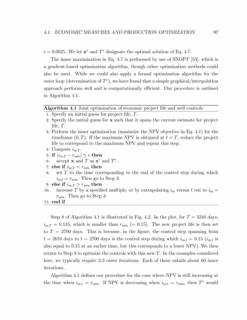
4.1. ECONOMIC MEASURES AND PRODUCTION OPTIMIZATION 97
ε = 0.0025. We let x∗ and T ∗ designate the optimal solution of Eq. 4.7.
The inner maximization in Eq. 4.7 is performed by use of SNOPT [53], which is
a gradient-based optimization algorithm, though other optimization methods could
also be used. While we could also apply a formal optimization algorithm for the
outer loop (determination of T ∗), we have found that a simple graphical/interpolation
approach performs well and is computationally efficient. Our procedure is outlined
in Algorithm 4.1.
Algorithm 4.1 Joint optimization of economic project life and well controls
1: Specify an initial guess for project life, T .2: Specify the initial guess for x such that it spans the current estimate for project
life, T .3: Perform the inner optimization (maximize the NPV objective in Eq. 4.1) for the
timeframe (0, T ). If the maximum NPV is obtained at t < T , reduce the projectlife to correspond to the maximum NPV and repeat this step.
4: Compute im,T .5: if |im,T − rmin| ≤ ε then6: accept x and T as x∗ and T ∗.7: else if im,T < rmin then8: set T to the time corresponding to the end of the control step during which
im,t = rmin. Then go to Step 3.9: else if im,T > rmin then
10: increase T by a specified multiple, or by extrapolating im versus t out to im =rmin. Then go to Step 3.
11: end if
Step 8 of Algorithm 4.1 is illustrated in Fig. 4.2. In the plot, for T = 3240 days,
im,T = 0.135, which is smaller than rmin (= 0.15). The new project life is then set
to T = 2700 days. This is because, in the figure, the control step spanning from
t = 2610 days to t = 2700 days is the control step during which im,t = 0.15 (im,t is
also equal to 0.15 at an earlier time, but this corresponds to a lower NPV). We then
return to Step 3 to optimize the controls with this new T . In the examples considered
here, we typically require 2-3 outer iterations. Each of these entails about 60 inner
iterations.
Algorithm 4.1 defines our procedure for the case where NPV is still increasing at
the time when im,t = rmin. If NPV is decreasing when im,t = rmin, then T ∗ would
98 CHAPTER 4. OPTIMIZATION OF ECONOMIC PROJECT LIFE
correspond to the time when NPV is a maximum. We have not observed this behavior
in any of our runs, but it could occur if capital costs are very low. There may be
other situations, such as those exhibiting one or more local maximums in NPV, for
which additional modification of Algorithm 4.1 is required.
4.2 Computational results
In this section, we present computational results for two different examples where
we apply our procedure to determine EPL and optimal BHPs. Both examples in-
volve two-phase oil-water flow. Oil and water viscosities are specified as 3 cp and
1 cp, respectively, and both fluids are considered to be incompressible. The rock
compressibility is specified to be 10−3 bar−1. Relative permeability curves are the
same as those used in Chapter 3 (Fig. 3.2). The reservoir initially contains oil and
connate water, with irreducible water saturation of Swc = 0.1. Deterministic opti-
mization (with a single realization) is considered in both cases. Flow simulations are
performed with Stanford’s AD-GPRS [157]. We apply the adjoint method within
AD-GPRS to compute the gradient of NPV with respect to the controls.
4.2.1 Example 4.1: 2D bimodal reservoir
The reservoir model in this example is two-dimensional and contains 100× 100 grid
blocks. The grid block dimensions are ∆x = ∆y = 100 ft, ∆z = 15 ft. The isotropic
log-permeability field, shown in Fig. 4.3, displays a bimodal distribution. The two
modes are of mean (in log-permeability) of 8 for the sand facies and 3 for shale facies,
with corresponding variances of 0.4 and 0.8. Porosity of the sand facies is equal to
0.2 and for the shale facies it is 0.1. There are 12 producers and six water injection
wells in this reservoir. All wells are operated under BHP control. Initial reservoir
pressure is 310 bar. Optimization parameters are shown in Table 4.1. The maximum
injection and total liquid production rates for a well are specified to 10,000 STBD.
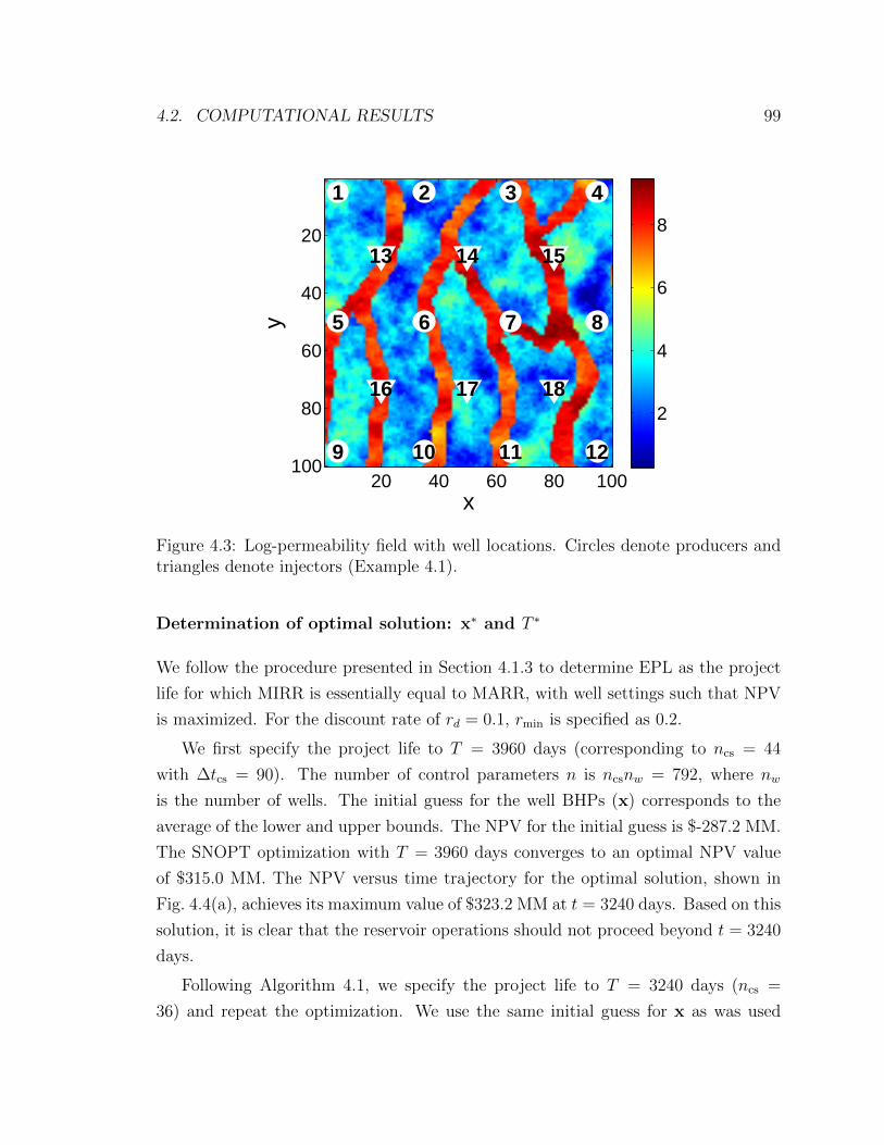
4.2. COMPUTATIONAL RESULTS 99
x
y
1 2 3 4
5 6 7 8
9 10 11 12
13 14 15
16 17 18
20 40 60 80 100
20
40
60
80
100
2
4
6
8
Figure 4.3: Log-permeability field with well locations. Circles denote producers andtriangles denote injectors (Example 4.1).
Determination of optimal solution: x∗ and T ∗
We follow the procedure presented in Section 4.1.3 to determine EPL as the project
life for which MIRR is essentially equal to MARR, with well settings such that NPV
is maximized. For the discount rate of rd = 0.1, rmin is specified as 0.2.
We first specify the project life to T = 3960 days (corresponding to ncs = 44
with ∆tcs = 90). The number of control parameters n is ncsnw = 792, where nw
is the number of wells. The initial guess for the well BHPs (x) corresponds to the
average of the lower and upper bounds. The NPV for the initial guess is $-287.2 MM.
The SNOPT optimization with T = 3960 days converges to an optimal NPV value
of $315.0 MM. The NPV versus time trajectory for the optimal solution, shown in
Fig. 4.4(a), achieves its maximum value of $323.2 MM at t = 3240 days. Based on this
solution, it is clear that the reservoir operations should not proceed beyond t = 3240
days.
Following Algorithm 4.1, we specify the project life to T = 3240 days (ncs =
36) and repeat the optimization. We use the same initial guess for x as was used
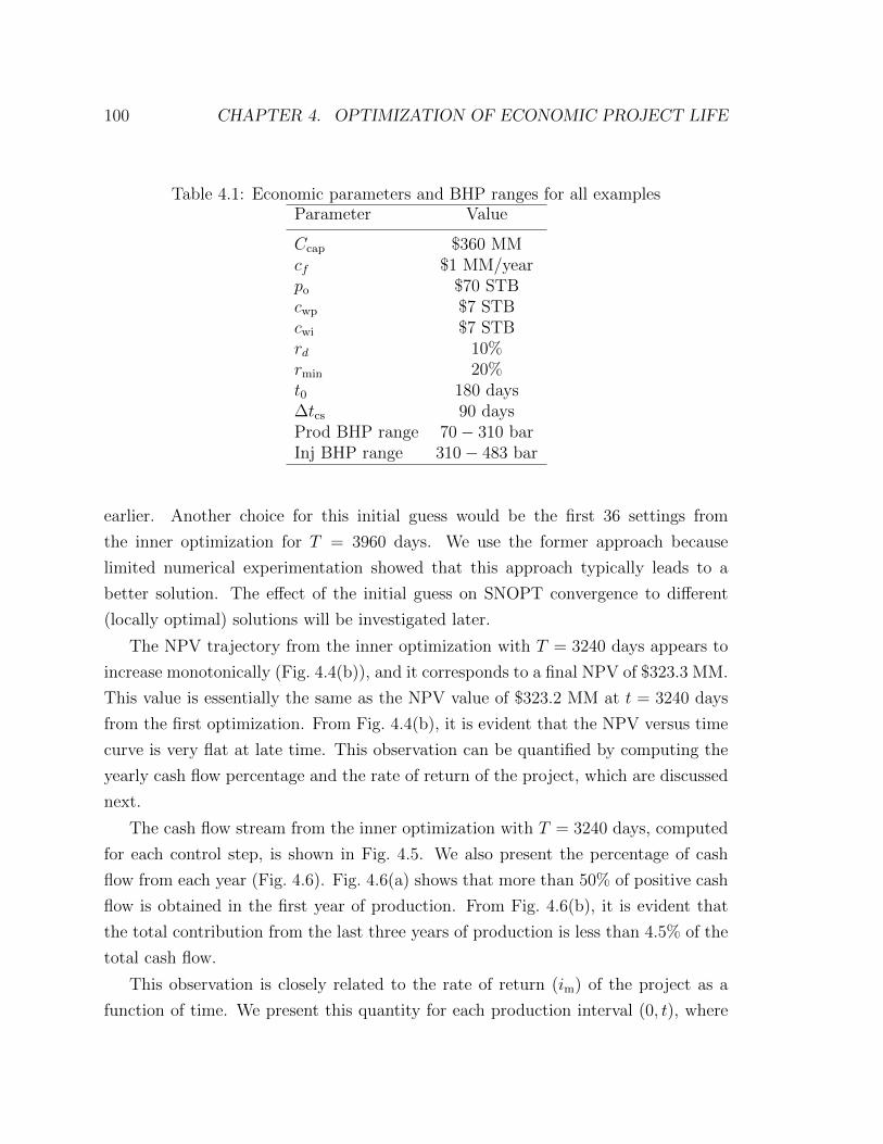
100 CHAPTER 4. OPTIMIZATION OF ECONOMIC PROJECT LIFE
Table 4.1: Economic parameters and BHP ranges for all examplesParameter Value
Ccap $360 MMcf $1 MM/yearpo $70 STBcwp $7 STBcwi $7 STBrd 10%rmin 20%t0 180 days∆tcs 90 daysProd BHP range 70− 310 barInj BHP range 310− 483 bar
earlier. Another choice for this initial guess would be the first 36 settings from
the inner optimization for T = 3960 days. We use the former approach because
limited numerical experimentation showed that this approach typically leads to a
better solution. The effect of the initial guess on SNOPT convergence to different
(locally optimal) solutions will be investigated later.
The NPV trajectory from the inner optimization with T = 3240 days appears to
increase monotonically (Fig. 4.4(b)), and it corresponds to a final NPV of $323.3 MM.
This value is essentially the same as the NPV value of $323.2 MM at t = 3240 days
from the first optimization. From Fig. 4.4(b), it is evident that the NPV versus time
curve is very flat at late time. This observation can be quantified by computing the
yearly cash flow percentage and the rate of return of the project, which are discussed
next.
The cash flow stream from the inner optimization with T = 3240 days, computed
for each control step, is shown in Fig. 4.5. We also present the percentage of cash
flow from each year (Fig. 4.6). Fig. 4.6(a) shows that more than 50% of positive cash
flow is obtained in the first year of production. From Fig. 4.6(b), it is evident that
the total contribution from the last three years of production is less than 4.5% of the
total cash flow.
This observation is closely related to the rate of return (im) of the project as a
function of time. We present this quantity for each production interval (0, t), where
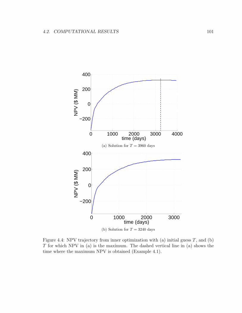
4.2. COMPUTATIONAL RESULTS 101
0 1000 2000 3000 4000
−200
0
200
400
time (days)
NP
V (
$ M
M)
(a) Solution for T = 3960 days
0 1000 2000 3000
−200
0
200
400
time (days)
NP
V (
$ M
M)
(b) Solution for T = 3240 days
Figure 4.4: NPV trajectory from inner optimization with (a) initial guess T , and (b)T for which NPV in (a) is the maximum. The dashed vertical line in (a) shows thetime where the maximum NPV is obtained (Example 4.1).
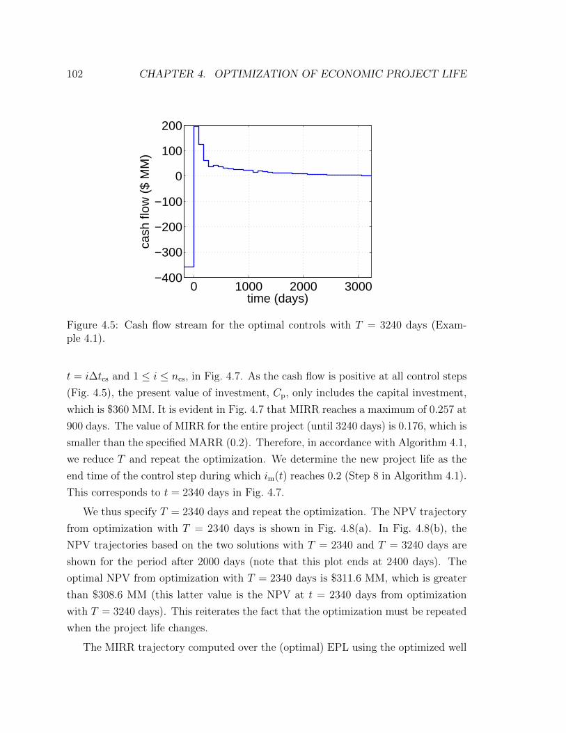
102 CHAPTER 4. OPTIMIZATION OF ECONOMIC PROJECT LIFE
0 1000 2000 3000−400
−300
−200
−100
0
100
200
time (days)
cash
flow
($
MM
)
Figure 4.5: Cash flow stream for the optimal controls with T = 3240 days (Exam-ple 4.1).
t = i∆tcs and 1 ≤ i ≤ ncs, in Fig. 4.7. As the cash flow is positive at all control steps
(Fig. 4.5), the present value of investment, Cp, only includes the capital investment,
which is $360 MM. It is evident in Fig. 4.7 that MIRR reaches a maximum of 0.257 at
900 days. The value of MIRR for the entire project (until 3240 days) is 0.176, which is
smaller than the specified MARR (0.2). Therefore, in accordance with Algorithm 4.1,
we reduce T and repeat the optimization. We determine the new project life as the
end time of the control step during which im(t) reaches 0.2 (Step 8 in Algorithm 4.1).
This corresponds to t = 2340 days in Fig. 4.7.
We thus specify T = 2340 days and repeat the optimization. The NPV trajectory
from optimization with T = 2340 days is shown in Fig. 4.8(a). In Fig. 4.8(b), the
NPV trajectories based on the two solutions with T = 2340 and T = 3240 days are
shown for the period after 2000 days (note that this plot ends at 2400 days). The
optimal NPV from optimization with T = 2340 days is $311.6 MM, which is greater
than $308.6 MM (this latter value is the NPV at t = 2340 days from optimization
with T = 3240 days). This reiterates the fact that the optimization must be repeated
when the project life changes.
The MIRR trajectory computed over the (optimal) EPL using the optimized well

4.2. COMPUTATIONAL RESULTS 103
1000 2000 30000
20
40
60
time (days)
% o
f tot
al p
ositi
ve c
ash
flow
(a) T = 3240 days
2200 2400 2600 2800 3000 32000
1
2
3
4
5
time (days)
% o
f tot
al p
ositi
ve c
ash
flow
(b) t ≥ 2160 days
Figure 4.6: (a) Cash flow percentage, computed yearly, versus time for optimal con-trols with T = 3240 days, and (b) magnification for the last three years (Example 4.1).
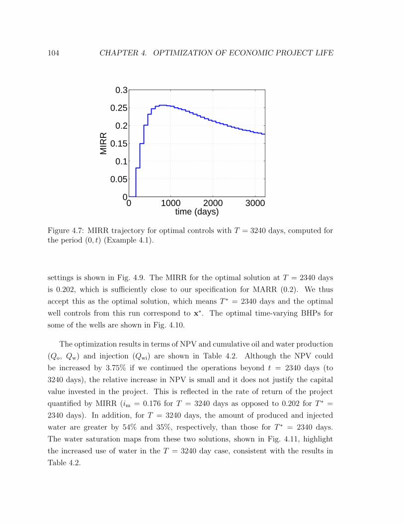
104 CHAPTER 4. OPTIMIZATION OF ECONOMIC PROJECT LIFE
0 1000 2000 30000
0.05
0.1
0.15
0.2
0.25
0.3
time (days)
MIR
R
Figure 4.7: MIRR trajectory for optimal controls with T = 3240 days, computed forthe period (0, t) (Example 4.1).
settings is shown in Fig. 4.9. The MIRR for the optimal solution at T = 2340 days
is 0.202, which is sufficiently close to our specification for MARR (0.2). We thus
accept this as the optimal solution, which means T ∗ = 2340 days and the optimal
well controls from this run correspond to x∗. The optimal time-varying BHPs for
some of the wells are shown in Fig. 4.10.
The optimization results in terms of NPV and cumulative oil and water production
(Qo, Qw) and injection (Qwi) are shown in Table 4.2. Although the NPV could
be increased by 3.75% if we continued the operations beyond t = 2340 days (to
3240 days), the relative increase in NPV is small and it does not justify the capital
value invested in the project. This is reflected in the rate of return of the project
quantified by MIRR (im = 0.176 for T = 3240 days as opposed to 0.202 for T ∗ =
2340 days). In addition, for T = 3240 days, the amount of produced and injected
water are greater by 54% and 35%, respectively, than those for T ∗ = 2340 days.
The water saturation maps from these two solutions, shown in Fig. 4.11, highlight
the increased use of water in the T = 3240 day case, consistent with the results in
Table 4.2.
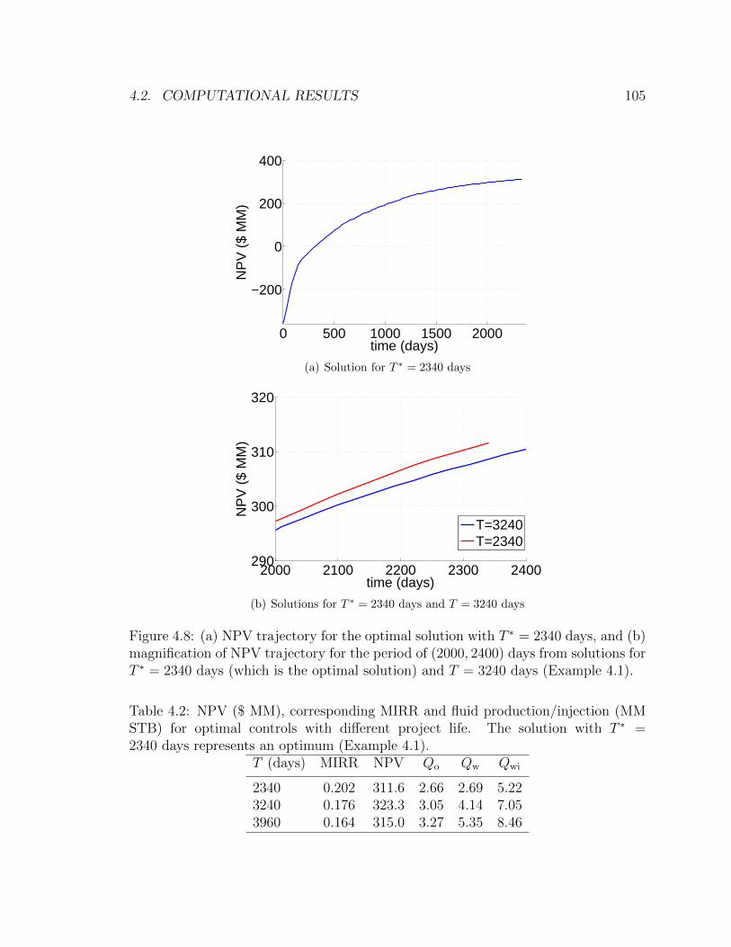
4.2. COMPUTATIONAL RESULTS 105
0 500 1000 1500 2000
−200
0
200
400
time (days)
NP
V (
$ M
M)
(a) Solution for T ∗ = 2340 days
2000 2100 2200 2300 2400290
300
310
320
time (days)
NP
V (
$ M
M)
T=3240T=2340
(b) Solutions for T ∗ = 2340 days and T = 3240 days
Figure 4.8: (a) NPV trajectory for the optimal solution with T ∗ = 2340 days, and (b)magnification of NPV trajectory for the period of (2000, 2400) days from solutions forT ∗ = 2340 days (which is the optimal solution) and T = 3240 days (Example 4.1).
Table 4.2: NPV ($ MM), corresponding MIRR and fluid production/injection (MMSTB) for optimal controls with different project life. The solution with T ∗ =2340 days represents an optimum (Example 4.1).
T (days) MIRR NPV Qo Qw Qwi
2340 0.202 311.6 2.66 2.69 5.223240 0.176 323.3 3.05 4.14 7.053960 0.164 315.0 3.27 5.35 8.46

106 CHAPTER 4. OPTIMIZATION OF ECONOMIC PROJECT LIFE
0 500 1000 1500 20000
0.05
0.1
0.15
0.2
0.25
0.3
time (days)
MIR
R
Figure 4.9: MIRR trajectory for the optimal solution (T ∗ = 2340 days) computed forthe period (0, t).
0 1000 2000
100
200
300
Time (Days)
BH
P(b
ar)
Well 2Well 6Well 8
(a) producers
0 1000 2000300
350
400
450
Time (Days)
BH
P(b
ar)
Well 13Well 15Well 16
(b) injectors
Figure 4.10: Optimal controls x∗ for three producers and three injectors correspondingto T ∗ = 2340 days (Example 4.1).
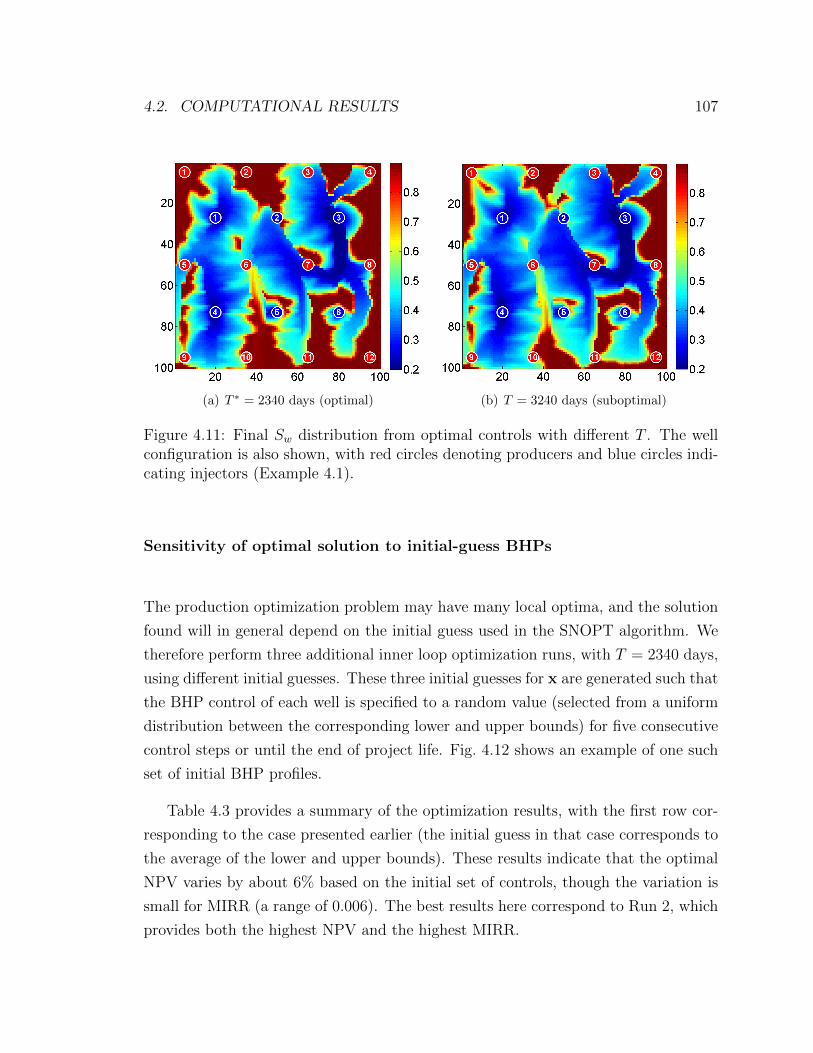
4.2. COMPUTATIONAL RESULTS 107
(a) T ∗ = 2340 days (optimal) (b) T = 3240 days (suboptimal)
Figure 4.11: Final Sw distribution from optimal controls with different T . The wellconfiguration is also shown, with red circles denoting producers and blue circles indi-cating injectors (Example 4.1).
Sensitivity of optimal solution to initial-guess BHPs
The production optimization problem may have many local optima, and the solution
found will in general depend on the initial guess used in the SNOPT algorithm. We
therefore perform three additional inner loop optimization runs, with T = 2340 days,
using different initial guesses. These three initial guesses for x are generated such that
the BHP control of each well is specified to a random value (selected from a uniform
distribution between the corresponding lower and upper bounds) for five consecutive
control steps or until the end of project life. Fig. 4.12 shows an example of one such
set of initial BHP profiles.
Table 4.3 provides a summary of the optimization results, with the first row cor-
responding to the case presented earlier (the initial guess in that case corresponds to
the average of the lower and upper bounds). These results indicate that the optimal
NPV varies by about 6% based on the initial set of controls, though the variation is
small for MIRR (a range of 0.006). The best results here correspond to Run 2, which
provides both the highest NPV and the highest MIRR.
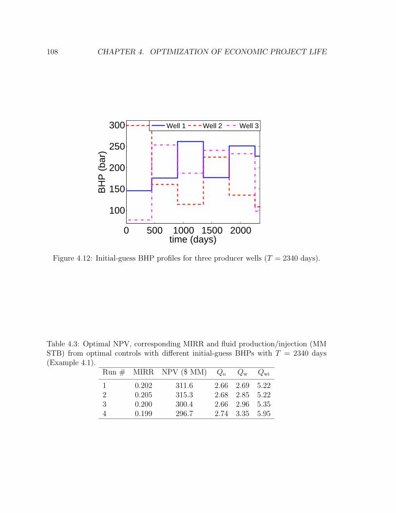
108 CHAPTER 4. OPTIMIZATION OF ECONOMIC PROJECT LIFE
0 500 1000 1500 2000
100
150
200
250
300
time (days)
BH
P (
bar)
Well 1 Well 2 Well 3
Figure 4.12: Initial-guess BHP profiles for three producer wells (T = 2340 days).
Table 4.3: Optimal NPV, corresponding MIRR and fluid production/injection (MMSTB) from optimal controls with different initial-guess BHPs with T = 2340 days(Example 4.1).
Run # MIRR NPV ($ MM) Qo Qw Qwi
1 0.202 311.6 2.66 2.69 5.222 0.205 315.3 2.68 2.85 5.223 0.200 300.4 2.66 2.96 5.354 0.199 296.7 2.74 3.35 5.95
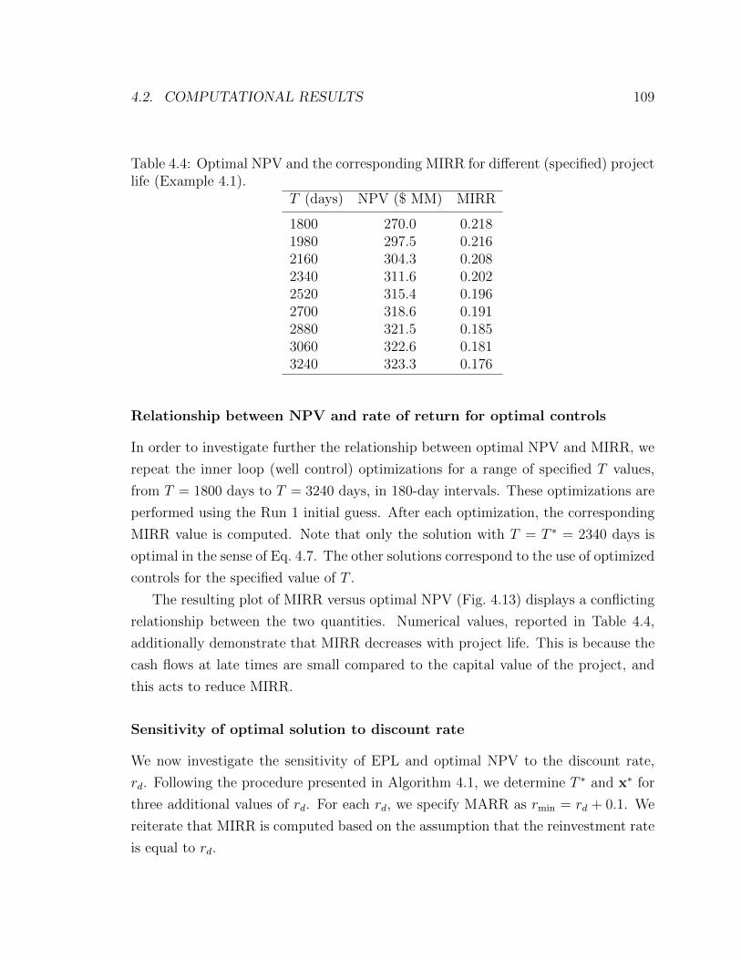
4.2. COMPUTATIONAL RESULTS 109
Table 4.4: Optimal NPV and the corresponding MIRR for different (specified) projectlife (Example 4.1).
T (days) NPV ($ MM) MIRR
1800 270.0 0.2181980 297.5 0.2162160 304.3 0.2082340 311.6 0.2022520 315.4 0.1962700 318.6 0.1912880 321.5 0.1853060 322.6 0.1813240 323.3 0.176
Relationship between NPV and rate of return for optimal controls
In order to investigate further the relationship between optimal NPV and MIRR, we
repeat the inner loop (well control) optimizations for a range of specified T values,
from T = 1800 days to T = 3240 days, in 180-day intervals. These optimizations are
performed using the Run 1 initial guess. After each optimization, the corresponding
MIRR value is computed. Note that only the solution with T = T ∗ = 2340 days is
optimal in the sense of Eq. 4.7. The other solutions correspond to the use of optimized
controls for the specified value of T .
The resulting plot of MIRR versus optimal NPV (Fig. 4.13) displays a conflicting
relationship between the two quantities. Numerical values, reported in Table 4.4,
additionally demonstrate that MIRR decreases with project life. This is because the
cash flows at late times are small compared to the capital value of the project, and
this acts to reduce MIRR.
Sensitivity of optimal solution to discount rate
We now investigate the sensitivity of EPL and optimal NPV to the discount rate,
rd. Following the procedure presented in Algorithm 4.1, we determine T ∗ and x∗ for
three additional values of rd. For each rd, we specify MARR as rmin = rd + 0.1. We
reiterate that MIRR is computed based on the assumption that the reinvestment rate
is equal to rd.
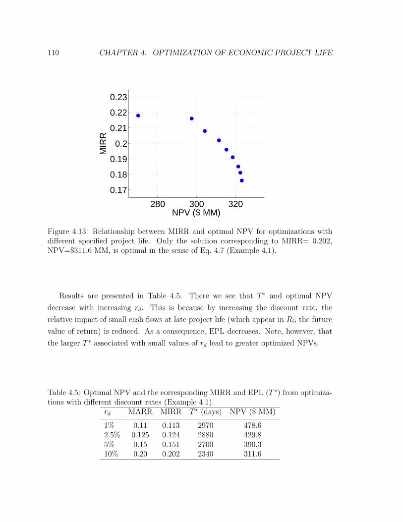
110 CHAPTER 4. OPTIMIZATION OF ECONOMIC PROJECT LIFE
280 300 320
0.17
0.18
0.19
0.2
0.21
0.22
0.23
NPV ($ MM)
MIR
R
Figure 4.13: Relationship between MIRR and optimal NPV for optimizations withdifferent specified project life. Only the solution corresponding to MIRR= 0.202,NPV=$311.6 MM, is optimal in the sense of Eq. 4.7 (Example 4.1).
Results are presented in Table 4.5. There we see that T ∗ and optimal NPV
decrease with increasing rd. This is because by increasing the discount rate, the
relative impact of small cash flows at late project life (which appear in Rf, the future
value of return) is reduced. As a consequence, EPL decreases. Note, however, that
the larger T ∗ associated with small values of rd lead to greater optimized NPVs.
Table 4.5: Optimal NPV and the corresponding MIRR and EPL (T ∗) from optimiza-tions with different discount rates (Example 4.1).
rd MARR MIRR T ∗ (days) NPV ($ MM)
1% 0.11 0.113 2970 478.62.5% 0.125 0.124 2880 429.85% 0.15 0.151 2700 390.310% 0.20 0.202 2340 311.6

4.2. COMPUTATIONAL RESULTS 111
4.2.2 Example 4.2: 3D binary reservoir
This example involves a three-dimensional binary channelized reservoir model, defined
on a grid of dimensions 50 × 50 × 6 (see Fig. 4.14). The grid block dimensions are
∆x = ∆y = 100 ft, ∆z = 15 ft. The isotropic horizonal permeabilities for sand and
shale are, respectively, 500 mD and 10 mD. The ratio of vertical permeability to
horizontal permeability is specified to be constant and equal to 0.2. The sand and
shale porosity are 0.2 and 0.1, respectively. There are five horizontal producers (in
Layers 1 and 2) and six vertical injectors (in Layers 4-6), as shown in Fig. 4.14. The
initial reservoir pressure is 310 bar.
The capital investment of the project is specified to be Ccap = $700 MM. The
discount rate is rd = 0.1, while the time lag between investment and the start of
production is t0 = 180 days. MARR is specified to be 0.2. Other optimization and
simulation parameters are identical to those in Example 4.1 (e.g., ∆tcs = 90 days).
We follow the procedure presented in Algorithm 4.1 to determine the optimal EPL
and optimal controls. We first specify T = 4950 days and optimize the NPV objective.
The NPV and MIRR trajectories are shown in Figs. 4.15 and 4.16. The maximum
NPV ($850 MM) is obtained at 4050 days. The value of MIRR at T = 4950 days is
0.164, which is smaller than 0.2. The control step where MIRR becomes less than
0.2 extends from 2970 days to 3060 days. Therefore, we specify the project life to
T = 3060 days and repeat the well control optimization.
The optimal NPV (at convergence of SNOPT) is $822 MM for T = 3060 days. As
Fig. 4.17 shows, the value of MIRR at T = 3060 days is equal to 0.200, which is the
exact value of MARR. Thus we have reached the optimum, meaning T ∗ = 3060 days
and the well controls associated with the result in Fig. 4.17 correspond to x∗. The
final water saturation maps for the optimal controls and optimal project life are
shown in Fig. 4.18. As none of the injectors is perforated in the top three layers,
Layer 1 displays large regions of unswept oil. Most of the other layers, however, show
a reasonable degree of sweep.
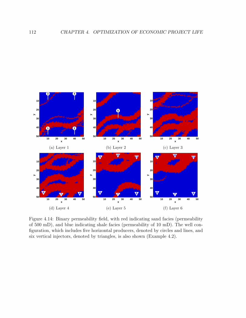
112 CHAPTER 4. OPTIMIZATION OF ECONOMIC PROJECT LIFE
x
y
1 2
3 4
Layer 1
10 20 30 40 50
10
20
30
40
50 0
0.2
0.4
0.6
0.8
1
(a) Layer 1
x
y
5
Layer 2
10 20 30 40 50
10
20
30
40
50 0
0.2
0.4
0.6
0.8
1
(b) Layer 2
x
y
Layer 3
10 20 30 40 50
10
20
30
40
50 0
0.2
0.4
0.6
0.8
1
(c) Layer 3
x
y
67 8
Layer 4
10 20 30 40 50
10
20
30
40
50 0
0.2
0.4
0.6
0.8
1
(d) Layer 4
x
y
67 8
910
11
Layer 5
10 20 30 40 50
10
20
30
40
50 0
0.2
0.4
0.6
0.8
1
(e) Layer 5
x
y
67 8
910
11
Layer 6
10 20 30 40 50
10
20
30
40
50 0
0.2
0.4
0.6
0.8
1
(f) Layer 6
Figure 4.14: Binary permeability field, with red indicating sand facies (permeabilityof 500 mD), and blue indicating shale facies (permeability of 10 mD). The well con-figuration, which includes five horizontal producers, denoted by circles and lines, andsix vertical injectors, denoted by triangles, is also shown (Example 4.2).
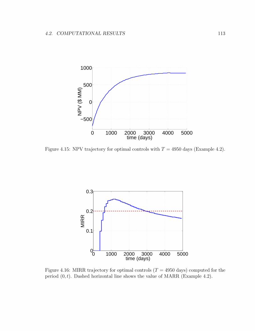
4.2. COMPUTATIONAL RESULTS 113
0 1000 2000 3000 4000 5000
−500
0
500
1000
time (days)
NP
V (
$ M
M)
Figure 4.15: NPV trajectory for optimal controls with T = 4950 days (Example 4.2).
0 1000 2000 3000 4000 50000
0.1
0.2
0.3
time (days)
MIR
R
Figure 4.16: MIRR trajectory for optimal controls (T = 4950 days) computed for theperiod (0, t). Dashed horizontal line shows the value of MARR (Example 4.2).
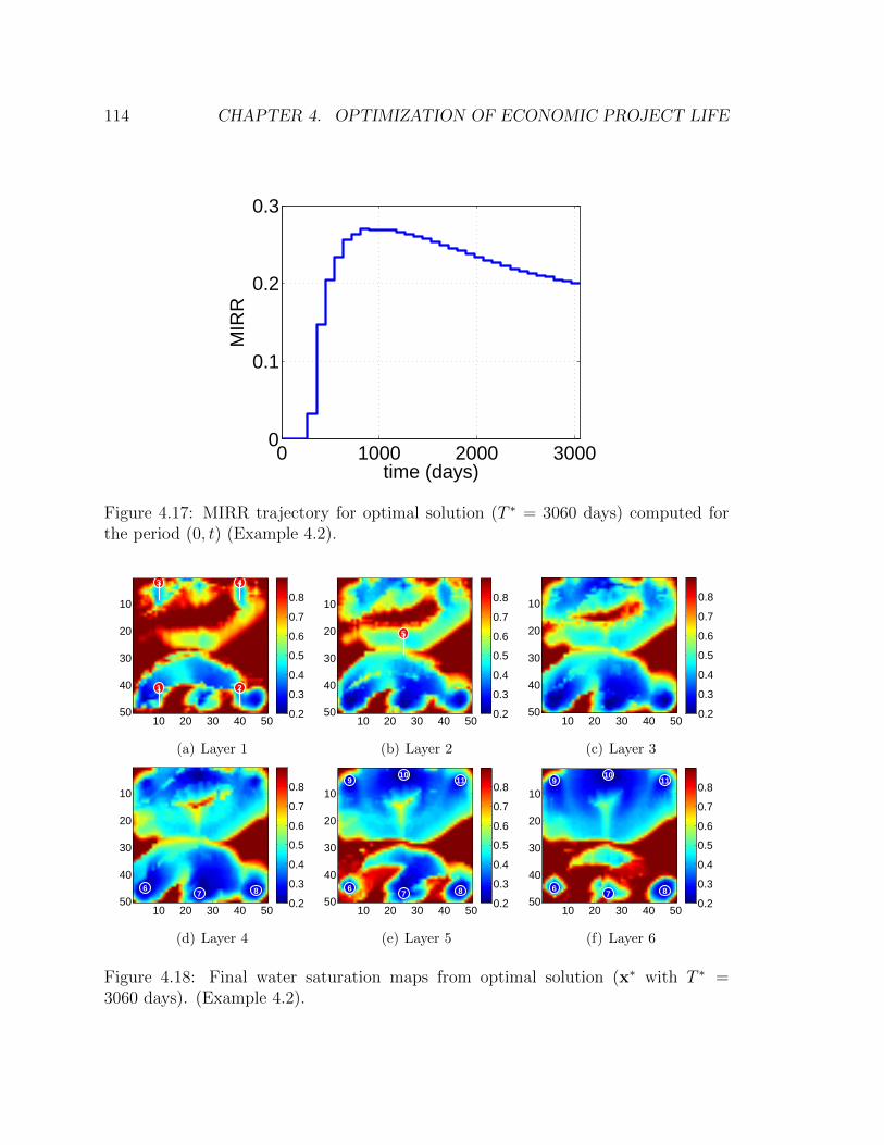
114 CHAPTER 4. OPTIMIZATION OF ECONOMIC PROJECT LIFE
0 1000 2000 30000
0.1
0.2
0.3
time (days)
MIR
R
Figure 4.17: MIRR trajectory for optimal solution (T ∗ = 3060 days) computed forthe period (0, t) (Example 4.2).
Layer 1, 3060 Days
1 2
3 4
10 20 30 40 50
10
20
30
40
50 0.2
0.3
0.4
0.5
0.6
0.7
0.8
(a) Layer 1
Layer 2, 3060 Days
5
10 20 30 40 50
10
20
30
40
50 0.2
0.3
0.4
0.5
0.6
0.7
0.8
(b) Layer 2
Layer 3, 3060 Days
10 20 30 40 50
10
20
30
40
50 0.2
0.3
0.4
0.5
0.6
0.7
0.8
(c) Layer 3Layer 4, 3060 Days
67 8
10 20 30 40 50
10
20
30
40
50 0.2
0.3
0.4
0.5
0.6
0.7
0.8
(d) Layer 4
Layer 5, 3060 Days
67 8
910
11
10 20 30 40 50
10
20
30
40
50 0.2
0.3
0.4
0.5
0.6
0.7
0.8
(e) Layer 5
Layer 6, 3060 Days
67 8
910
11
10 20 30 40 50
10
20
30
40
50 0.2
0.3
0.4
0.5
0.6
0.7
0.8
(f) Layer 6
Figure 4.18: Final water saturation maps from optimal solution (x∗ with T ∗ =3060 days). (Example 4.2).
4.3. SUMMARY 115
4.3 Summary
In this chapter, we introduced a procedure for the simultaneous determination of
optimal project life (referred to as economic project life, EPL) and optimal well
controls. Because the optimal controls depend on the specified project life T , the
optimal controls must be recomputed if T is varied. We formulated this problem as
a nested optimization in which we maximize NPV while requiring that the modified
internal rate of return of the project is (essentially) equal to the minimum attractive
rate of return (MARR or hurdle rate). The outer loop of the optimization entails
optimization of T , while the inner loop involves optimization of the controls given the
current T . We successfully applied the methodology for determining optimal EPL
and optimal controls to two examples involving a two-dimensional bimodal reservoir
model and a three-dimensional binary model with horizontal production wells.
In this work we only considered deterministic optimization (with a single real-
ization). The methodology, however, can be extended for optimization under un-
certainty. For multiple realizations, the optimization with sample validation (OSV)
framework (presented in Chapter 2) can be applied to accelerate the computations.
The realization selection method, presented in Chapter 3, can be used within the
OSV framework. Computation of rate of return for multiple realizations, however,
may require additional treatments, such as those presented by Hazen [61].

116 CHAPTER 4. OPTIMIZATION OF ECONOMIC PROJECT LIFE
Chapter 5
Summary, Conclusions and Future
Work
In this work, we introduced and applied advanced techniques relevant for reservoir op-
timization under uncertainty. We first developed a general framework for closed-loop
field development optimization under uncertainty that incorporates data from new
wells as they are drilled. We then investigated two particular aspects of closed-loop
reservoir optimization as standalone topics. These include selecting a representa-
tive subset from a large set of geological realizations and the joint optimization of
economic project life (EPL) and well settings.
5.1 Conclusions
The key contributions from our work on closed-loop field development (CLFD) are
as follows:
• We introduced a general methodology for closed-loop field development (CLFD).
The framework includes optimization, data collection and history matching per-
formed in a repeated sequence. Uncertainty is taken into account by history
matching, and optimizing over, multiple geological realizations. The optimiza-
tion step, which uses the recently developed PSO-MADS hybrid algorithm,
allows the determination of well type, locations and controls for new wells, and
117
118 CHAPTER 5. SUMMARY, CONCLUSIONS AND FUTURE WORK
(future) well controls for existing wells. The history matching step entails the
use of the RML method, which is applied within an adjoint-gradient setting
using AD-GPRS.
• A key feature of CLFD is that, at each optimization step, the full development
plan is optimized, i.e., the location of each well is determined based on the
fact that it is one well in a sequence. The future field development plan (type,
locations and controls for planned wells) does, however, change as new data are
collected.
• We showed that a greedy approach for field development optimization, in which
the location, type and controls of each well are optimized independently (one
at a time), may lead to a suboptimal solution. This further motivates the need
to optimize the parameters associated with all wells simultaneously.
• We introduced an optimization with sample validation (OSV) procedure as
a computationally efficient means for optimizing under geological uncertainty.
In OSV, the optimization at each CLFD step is first performed on a (small)
subset of representative realizations. A validation step is then applied to assess
(quantitatively) whether the selected subset is sufficiently representative of the
entire set of realizations. If not, a larger subset of realizations is selected and the
CLFD optimization step is repeated. At each OSV step, a representative subset
of realizations was reselected based on the NPVs computed using the current
best field development plan, though other flow or permeability information could
also be used for this selection.
Recently, Aliyev and Durlofsky [4] incorporated the OSV procedure in their
multilevel optimization approach to accelerate the joint optimization of well
locations and controls under geological uncertainty.
• We presented appropriate CLFD history matching treatments for (Gaussian)
models described by two-point geostatistics and channelized models described
by multipoint geostatistics. The CLFD procedure for channelized models, pre-
sented in Appendix A, involves a two-stage conditioning where hard data are
5.1. CONCLUSIONS 119
first incorporated by use of geostatistical simulation, and then production data
are integrated through O-PCA-based history matching.
Our main findings regarding the selection of representative models are:
• We developed and tested a new framework for selecting a representative subset
of realizations from a large set, for the purpose of optimization or decision mak-
ing under uncertainty. A low-dimensional flow-response vector was defined to
efficiently quantify base-case flow simulation results for a particular realization,
and principal component analysis was applied to concisely represent the het-
erogeneous permeability field. We introduced a clustering algorithm that can
use flow-based or geology-based information, or a combination of the two (with
arbitrary weightings), for realization selection.
• Three different realization-selection approaches, which can all be defined within
our overall framework, were applied for four different cases. These cases in-
volved the (separate) consideration of new well settings and new well locations,
and well-parameter vectors (which define new well settings or locations) that
were generated either randomly (as in PSO or GA), or through systematic per-
turbations around a base case (as in pattern search methods). The selection
methods were assessed in terms of the difference in flow response between the
selected subset and the full set of realizations. Many new well-parameter vec-
tors were considered, and results were expressed concisely in terms of median
performance. We found that, for all cases except for random configurations of
new wells, the use of clustering with flow-based information was clearly benefi-
cial. For random well configurations, the various selection approaches provided
similar performance, though all approaches outperformed random selection.
• We considered the use of both full-physics simulations as well as proxy (tracer-
type) flow information for obtaining flow-based features in clustering. Our
results showed that simplified (proxy) flow simulations provided a viable alter-
native for obtaining flow-based features for clustering for the cases considered.

120 CHAPTER 5. SUMMARY, CONCLUSIONS AND FUTURE WORK
• We investigated the use of representative subsets selected by the various ap-
proaches in production optimization under uncertainty. The optimization re-
sults were consistent with our findings for random or perturbation-based well-
parameter vectors, and demonstrated the benefit of using flow-based informa-
tion for realization selection.
Our work on the simultaneous determination of optimal operational settings and
optimal project life (EPL) leads us to the following observations:
• We introduced a nested formulation for the joint optimization of well controls
and economic project life (EPL), with EPL optimized in the outer loop, and
the associated well controls in the inner loop.
• Our methodology determines the optimal project life and well settings such that
the maximum NPV is obtained at the end of project life, and the rate of return
of the project is (essentially) equal to the hurdle rate or the minimum attractive
rate of return (MARR). This avoids situations with negligible increase in NPV
at late times.
• Our computational results indicated that increasing reservoir life may increase
the optimal NPV, but decrease the rate of return (as reflected by modified
internal rate of return). This highlights a fundamental trade off between these
two quantities.
5.2 Future work
There are many directions that could be pursued in areas relevant to CLFD. Our
suggestions for future research are as follows:
• Because the CLFD procedure is computationally demanding, it will be useful to
develop surrogate models to accelerate the optimization runs, or to implement
more efficient optimization methods.
• Value of information should also be included in CLFD. Relevant work in this
area has been presented in [15, 38].
5.2. FUTURE WORK 121
• In order to protect against downside risk due to geological uncertainty, bi-
objective optimization [69] could be incorporated into CLFD. We could then,
for example, minimize a risk objective while maximizing expected performance.
• In our current CLFD implementation, we assume the geological ‘scenario’ is
known and then consider uncertainty in the permeability distribution. It will
be of interest to consider situations where the geological scenario (i.e., training
image) is also uncertain and must be determined as part of the CLFD history
matching step. This could be accomplished using, e.g., the approach presented
by [107, 108].
• Treatments for accommodating 4D seismic data, in addition to production data,
should be introduced into the general CLFD framework.
• It will be useful to develop an adaptive realization-selection procedure that is
appropriate for use in challenging well placement (or joint well placement and
control) optimizations. Within the context of a hybrid stochastic – local search
algorithm, such as PSO–MADS, this would entail the use of different weightings
for flow versus permeability features as the optimization proceeds. Treatments
could also be devised for the nested optimization approach presented in [19]. In
this case, realizations could be selected based on the well locations prescribed
in the outer loop of the optimization.
• It will also be of interest to investigate the application of our selection ap-
proaches to realistic and more complex recovery processes involving, e.g., three-
phase flow or steam injection. Uncertainty in other simulation quantities, such
as relative permeability parameters, should also be considered.
• The procedures described here for selection of representative realizations should
be implemented within the CLFD framework. They could also be applied for
related subsurface flow problems such as CO2 sequestration or groundwater
management.
• In this work, we captured the flow response of a realization by dividing the
reservoir life into a few time intervals. It may be worth investigating the ap-
plication of functional data analysis (see, e.g., [105]) to define an alternative

122 CHAPTER 5. SUMMARY, CONCLUSIONS AND FUTURE WORK
flow-response vector that concisely captures flow simulation results.
• Our methodology for the joint optimization of project life and well controls
was presented for deterministic problems. It will be of interest to extend this
methodology to include multiple realizations. Treatments should be developed
to compute an appropriate rate of return when multiple realizations are consid-
ered.
• An approach for the joint optimization of well locations and control, together
with project life, could be developed. Along these lines, our method for the
joint optimization of project life and well controls can be incorporated in the
nested formulation of [19]. The inner optimization in this case will determine
the optimal well controls and project life, while the outer optimization provides
the well locations.

Nomenclature
Abbreviations
AD-GPRS Automatic Differentiation-based General Purpose Research Simulator
BHP bottom-hole pressure
CDF cumulative distribution function
CLFD closed-loop field development
CLRM closed-loop reservoir management
EPL economic project life
GA genetic algorithm
IRR internal rate of return
MADS mesh adaptive direct search
MAP maximum a posteriori
MARR minimum attractive rate of return
MIRR modified internal rate of return
NPV net present value
OSV optimization with sample validation
O-PCA optimization-based PCA
PCA principal component analysis
PDF probability density function
PSO particle swarm optimization
PS pattern search
RML randomized maximum likelihood
SCP sequential convex programming
SNOPT sparse nonlinear optimizer
STB stock tank barrels
123

124 NOMENCLATURE
STBD stock tank barrels per day
TSVD truncated singular value decomposition
Variables
cf fixed costs
cwi cost of injected water
cwp cost of produced water
C covariance matrix
Ccap capital investment
Cp present value of investment
Cw drilling cost per well
d dissimilarity measure between mean flow response vectors
D set of dissimilarity values between full set and a representative subset
d observed data
f cash flow at every simulation time step
Fcs cash flow at every control step
g simulated data
im modified internal rate of return (MIRR)
J net present value
J expected net present value
kro relative permeability for oil phase
krw relative permeability for water phase
l number of PCA parameters
L number of realizations for obtaining PCA parameters
mD median of set D
m geological realization
m mean of permeability realizations
M , M matrix of geological realizations
n number of decision parameters
nr number of representative realizations
ns maximum number of OSV subproblems
nw maximum number of wells

NOMENCLATURE 125
NI number of injector wells
NP number of producer wells
NR number of realizations in the full set
po oil price
q well flow response vector
Q total liquid production/injection
r flow-response vector
r mean flow-response vector
rd discount rate
rmin minimum attractive rate of return (MARR) or hurdle rate
Rf future value of return
RI relative improvement
S mismatch in history matching
SN normalized mismatch in history matching
Sw water saturation
t time
t0 time lag
T project life
T ∗ optimal economic project life (EPL)
U matrix of left singular vectors
V matrix of right singular vectors
x vector of decision variables
x∗ optimal well controls
Z feature matrix for clustering
Zf flow-based feature matrix for clustering
Zp permeability-based feature matrix for clustering
Z normalized feature matrix for clustering
Greek Symbols
α weighting factor for permeability-based features in clustering
Λ diagonal matrix of singular values
µ viscosity

126 NOMENCLATURE
θ validation criterion
ξ vector of PCA parameters
Subscripts/Superscripts
b number of base flow problems for obtaining flow-based features in clustering
cs control step
d data
full full set of geological realizations
h hard data
l lower bound
m median
m model
o oil
p production data
rep representative set of geological realizations
u upper bound
w water

Bibliography
[1] S. Afshari, B. Aminshahidy, and M. R. Pishvaie. Application of an improved
harmony search algorithm in well placement optimization using streamline sim-
ulation. Journal of Petroleum Science and Engineering, 78(3):664–678, 2011.
[2] I. Aitokhuehi and L. J. Durlofsky. Optimizing the performance of smart wells
in complex reservoirs using continuously updated geological models. Journal of
Petroleum Science and Engineering, 48(3):254–264, 2005.
[3] E. Aliyev and L. J. Durlofsky. Multilevel field-development optimization using a
sequence of upscaled models. Paper SPE 173198 presented at the SPE Reservoir
Simulation Symposium, Houston, Texas, USA, 2015.
[4] E. Aliyev and L. J. Durlofsky. Multilevel field development optimization under
uncertainty using a sequence of upscaled models. Mathematical Geosciences,
1–33, 2016, doi: 10.1007/s11004-016-9643-0.
[5] E. Aliyev. Multilevel Field Development Optimization Under Uncertainty Using
a Sequence of Upscaled Models. PhD thesis, Stanford University, 2015.
[6] D. Altshuler and C. A. Magni. Why IRR is not the rate of return for your
investment: Introducing AIRR to the real estate community. Journal of Real
Estate Portfolio Management, 18(2):219–230, 2012.
[7] E. Ansari. Mathematical Scaling and Statistical Modeling of Geopressured
Geothermal Reservoirs. PhD thesis, Louisiana State University, 2016.
127
128 BIBLIOGRAPHY
[8] E. Ansari and R. Hughes. Response surface method for assessing energy produc-
tion from geopressured geothermal reservoirs. Geothermal Energy, 4(1):4–15,
2016.
[9] E. Ansari, R. Hughes, and C. D. White. Well placement optimization for maxi-
mum energy recovery from hot saline aquifers. Proceedings of the Thirty-Ninth
Workshop on Geothermal Reservoir Engineering, Stanford, California, 2014.
[10] M. Armstrong, A. Ndiaye, R. Razanatsimba, and A. Galli. Scenario reduction
applied to geostatistical simulations. Mathematical Geosciences, 45(2):165–182,
2013.
[11] D. Arnold, V. Demyanov, M. Christie, A. Bakay, and K. Gopa. Optimisation
of decision making under uncertainty throughout field lifetime: A fractured
reservoir example. Computers & Geosciences, 95:123–139, 2016.
[12] V. Artus, L. J. Durlofsky, J. Onwunalu, and K. Aziz. Optimization of non-
conventional wells under uncertainty using statistical proxies. Computational
Geosciences, 10(4):389–404, 2006.
[13] C. Audet and J. Dennis Jr. Mesh adaptive direct search algorithms for con-
strained optimization. SIAM Journal on Optimization, 17(1):188–217, 2006.
[14] R. B. Balyeat, J. Cagle, and P. Glasgo. Teaching MIRR to improve comprehen-
sion of investment performance evaluation techniques. Journal of Economics
and Finance Education, 12(1):39–50, 2013.
[15] E. G. D. Barros, P. M. J. Van den Hof, and J. D. Jansen. Value of information in
closed-loop reservoir management. Computational Geosciences, 20(3):737–749,
2016.
[16] P. Bayer and M. Finkel. Optimization of concentration control by evolution
strategies: Formulation, application, and assessment of remedial solutions. Wa-
ter Resources Research, 43(2), 2007.
BIBLIOGRAPHY 129
[17] P. Bayer, C. Burger, and M. Finkel. Computationally efficient stochastic op-
timization using multiple realizations. Advances in Water Resources, 31(2):
399–417, 2008.
[18] P. Bayer, M. de Paly, and C. M. Burger. Optimization of high-reliability-based
hydrological design problems by robust automatic sampling of critical model
realizations. Water Resources Research, 46(5), 2010.
[19] M. C. Bellout, D. Echeverrıa Ciaurri, L. J. Durlofsky, B. Foss, and J. Kleppe.
Joint optimization of oil well placement and controls. Computational Geo-
sciences, 16(4):1061–1079, 2012.
[20] Z. Bouzarkouna, D. Y. Ding, and A. Auger. Well placement optimization with
the covariance matrix adaptation evolution strategy and meta-models. Compu-
tational Geosciences, 16(1):75–92, 2012.
[21] P. G. Brodrick, C. A. Kang, A. R. Brandt, and L. J. Durlofsky. Optimization
of carbon-capture-enabled coal-gas-solar power generation. Energy, 79:149–162,
2015.
[22] D. R. Brouwer and J. D. Jansen. Dynamic optimization of water flooding with
smart wells using optimial control theory. SPE Journal, 9(4):391–402, 2004.
[23] A. Y. Bukhamsin, M. M. Farshi, and K. Aziz. Optimization of multilateral well
design and location in a real field using a continuous genetic algorithm. Paper
SPE 136944 presented at the SPE Technical Symposium, Al-Khobar, Saudi
Arabia, 2010.
[24] V. Bukshtynov, O. Volkov, L. J. Durlofsky, and K. Aziz. Comprehensive
framework for gradient-based optimization in closed-loop reservoir manage-
ment. Computational Geosciences, 19(4):877–897, 2015.
[25] J. Caers. History matching under training-image-based geological model con-
straints. SPE Journal, 8(3):218–226, 2003.
130 BIBLIOGRAPHY
[26] D. A. Cameron and L. J. Durlofsky. Optimization and data assimilation for
geological carbon storage. In: R. Al-Khoury, J. Bundschuh (Eds.), Computa-
tional Models for CO2 Geo-sequestration & Compressed Air Energy Storage.
CRC Press, 355-388, 2014.
[27] D. A. Cameron and L. J. Durlofsky. Optimization of well placement, CO2 injec-
tion rates, and brine cycling for geological carbon sequestration. International
Journal of Greenhouse Gas Control, 10:100–112, 2012.
[28] S. A. Castro. A Probabilistic Approach to Jointly Integrate 3D/4D Seismic, Pro-
duction Data and Geological Information for Building Reservoir Models. PhD
thesis, Stanford University, 2007.
[29] C. Chen, G. Li, and A. Reynolds. Robust constrained optimization of short-
and long-term net present value for closed-loop reservoir management. SPE
Journal, 17(3):849–864, 2012.
[30] Y. Chen, D. S. Oliver, D. Zhang. Efficient ensemble-based closed-loop produc-
tion optimization. SPE Journal, 14(04):634–645, 2009.
[31] J. Cherry. Optimization Strategies for Shale Gas Asset Development. Master’s
thesis, Stanford University, 2016.
[32] H. Chipman and R. Tibshirani. Hybrid hierarchical clustering with applications
to microarray data. Biostatistics, 7(2):286–301, 2006.
[33] V. Dehdari, D. S. Oliver. Sequential quadratic programming for solving con-
strained production optimization–case study from Brugge field. SPE Journal,
17(3):874–884, 2012.
[34] S. Do. Application of SPSA-type Algorithms to Production Optimization. PhD
thesis, University of Tulsa, 2012.
[35] L. J. Durlofsky, R. C. Jones, and W. J. Milliken. A nonuniform coarsening
approach for the scale-up of displacement processes in heterogeneous porous
media. Advances in Water Resources, 20(5):335–347, 1997.
BIBLIOGRAPHY 131
[36] D. Echeverrıa Ciaurri, O. J. Isebor, and L. J. Durlofsky. Application of
derivative-free methodologies to generally constrained oil production optimisa-
tion problems. International Journal of Mathematical Modelling and Numerical
Optimisation, 2(2):134–161, 2011.
[37] D. Echeverrıa Ciaurri, T. Mukerji, E. T. Santos. Robust scheme for inversion
of seismic and production data for reservoir facies modeling. Paper SEG 2432
presented at the SEG Annual Meeting, Houston, Texas, USA, 2009.
[38] J. Eidsvik, T. Mukerji, and D. Bhattacharjya. Value of Information in the
Earth Sciences: Integrating Spatial Modeling and Decision Analysis. Cambridge
University Press, 2015.
[39] A. A. Emerick, E. Silva, B. Messer, L. F. Almeida, D. Szwarcman, M. Pacheco,
and M. Vellasco. Well placement optimization using a genetic algorithm with
nonlinear constraints. Paper SPE 118808 presented at the SPE Reservoir Sim-
ulation Symposium, The Woodlands, Texas, USA, 2009.
[40] A. A. Emerick and A. C. Reynolds. Ensemble smoother with multiple data
assimilation. Computers & Geosciences, 55:3–15, 2013.
[41] A. H. Elsheikh, M. F. Wheeler, I. Hoteit. Sparse calibration of subsurface flow
models using nonlinear orthogonal matching pursuit and an iterative stochastic
ensemble method. Advances in Water Resources, 56:14–26, 2013.
[42] Z. Fathi, F. W. Ramirez. Optimal injection policies for enhanced oil recovery:
part 2–surfactant flooding. SPE Journal, 24(3):333–341, 1984.
[43] R.M. Fonseca, O. Leeuwenburgh, P.M.J. Van den Hof, and J. D. Jansen.
Ensemble-based hierarchical multi-objective production optimization of smart
wells. Computational Geosciences, 18(3):449–461, 2014.
[44] L. A. Fonseca, E. R. Araujo, and S. M. Garcia. Simultaneous optimization
of well locations and control rates under geological uncertainty. International
Journal of Modeling and Simulation for the Petroleum Industry, 9(2):1–8, 2016.
132 BIBLIOGRAPHY
[45] T. Foroud, A. Seifi, and B. AminShahidy. An efficient optimization process for
hydrocarbon production in presence of geological uncertainty using a clustering
method: A case study on Brugge field. Journal of Natural Gas Science and
Engineering, 32:476–490, 2016.
[46] F. Forouzanfar and A. C. Reynolds. Joint optimization of number of wells, well
locations and controls using a gradient-based algorithm. Chemical Engineering
Research and Design, 92:1315–1328, 2013.
[47] A. Frooqnia, M. R. Pishvaie, and B. Aminshahidy. Real time optimization of a
natural gas lift system with a differential evaluation method. Energy Sources,
Part A: Recovery, Utilization, and Environmental Effects, 36(3):309–322, 2014.
[48] A. Frooqnia, C. T. Verdın, and K. Sepehrnoori. Inference of rock pressure-
production properties from gas-oil production logs. Journal of Natural Gas
Science and Engineering, 36(3):124-143, 2016.
[49] A. Frooqnia, C. T. Verdın, K. Sepehrnoori, and R. Abdhollah-Pour. Transient
coupled borehole/formation fluid-flow model for interpretation of oil/water pro-
duction logs. SPE Journal, 2016, doi: 10.2118/183628-PA.
[50] G. Gao, J. C. Vink, C. Chen, F. O. Alpak, and K. Du. A parallelized and
hybrid data-integration algorithm for history matching of geologically complex
reservoirs. SPE Journal, 2016, doi: 10.2118/175039-PA.
[51] G. Gao and A. C. Reynolds. An improved implementation of the LBFGS algo-
rithm for automatic history matching. SPE Journal, 11(1):5–17, 2006.
[52] H. Ghorbanidehno, A. Kokkinaki, J. Y. Li, E. Darve, and P. K. Kitanidis.
Real-time data assimilation for large-scale systems: The spectral Kalman filter.
Advances in Water Resources, 86:260–272, 2015.
[53] P. E. Gill, W. Murray, and M. A. Saunders. SNOPT: An SQP algorithm for
large-scale constrained optimization. SIAM Review, 47(1):99–131, 2005.

BIBLIOGRAPHY 133
[54] A. Golmohammadi, M. R. Khaninezhad, and B. Jafarpour. Group-sparsity
regularization for ill-posed subsurface flow inverse problems. Water Resources
Research, 51(10):8607–8626, 2015.
[55] A. D. Gordon and M. Vichi. Partitions of partitions. Journal of Classification,
15(2):265–285, 1998.
[56] B. Guyaguler, R. N. Horne, L. Rogers, J. J. Rosenzweig. Optimization of well
placement in a Gulf of Mexico waterflooding project. SPE Reservoir Evaluation
& Engineering, 5(3):229–236, 2002.
[57] J. A. Hartigan and M. A. Wong. Algorithm AS 136: A k-means clustering
algorithm. Journal of the Royal Statistical Society. Series C (Applied Statistics),
28(1): 100–108, 1979.
[58] J. C. Hartman and I. C. Schafrick. The relevant internal rate of return. The
Engineering Economist, 49(2):139–158, 2004.
[59] T. Hastie, R. Tibshirani, and J. Friedman. The Elements of Statistical Learning:
Data Mining, Inference, and Prediction, volume 2. Springer, 2009.
[60] G. B. Hazen. A new perspective on multiple internal rates of return. The
Engineering Economist, 48(1):31–51, 2003.
[61] G. Hazen. An extension of the internal rate of return to stochastic cash flows.
Management Science, 55(6):1030–1034, 2009.
[62] R. C. Higgins. Analysis for Financial Management (10th ed). McGraw-Hill,
2012.
[63] K. Hornik. A CLUE for CLUster Ensembles. Journal of Statistical Software,
14(12), September 2005. URL http://www.jstatsoft.org/v14/i12/.
[64] S. A. Hosseini, S. Kang, and A. Datta-Gupta. Qualitative well placement
and drainage volume calculations based on diffusive time of flight. Journal
of Petroleum Science and Engineering, 75(1):178–188, 2010.
134 BIBLIOGRAPHY
[65] T. D. Humphries, R. D. Haynes, and L. A. James. Simultaneous and sequential
approaches to joint optimization of well placement and control. Computational
Geosciences, 18(3):433–448, 2014.
[66] T. M. Hurley, X. Rao, and P. G. Pardey. Re-examining the reported rates of
return to food and agricultural research and development. American Journal
of Agricultural Economics, 96:1492–1504, 2014.
[67] F. Ibrahima. Probability Distribution Methods for Nonlinear Transport in Het-
erogeneous Porous Media. PhD thesis, Stanford University, 2016.
[68] F. Ibrahima, D. W. Meyer, and H. A. Tchelepi, Distribution functions of satu-
ration for stochastic nonlinear two-phase flow. Transport in Porous Media, 109
(1):81–107, 2015.
[69] O. J. Isebor and L. J. Durlofsky. Biobjective optimization for general oil field
development. Journal of Petroleum Science and Engineering, 119(18):123–138,
2014.
[70] O. J. Isebor, L. J. Durlofsky, and D. Echeverrıa Ciaurri. A derivative-free
methodology with local and global search for the constrained joint optimization
of well locations and controls. Computational Geosciences, 18:463–482, 2014.
[71] O. J. Isebor, D. Echeverrıa Ciaurri, and L. J. Durlofsky. Generalized field-
development optimization with derivative-free procedures. SPE Journal, 19:
891–908, 2014.
[72] O. J. Isebor. Constrained Production Optimization with an Emphasis on
Derivative-free Methods. Master’s thesis, Stanford University, 2009.
[73] O. J. Isebor. Derivative-free Optimization for Generalized Oil Field Develop-
ment. PhD thesis, Stanford University, 2013.
[74] A. Jahandideh and B. Jafarpour. Optimization of hydraulic fracturing design
under spatially variable shale fracability. Journal of Petroleum Science and
Engineering, 138:174–188, 2016.
BIBLIOGRAPHY 135
[75] J. D. Jansen, S. D. Douma, D. R. Brouwer, P. M. J. Van den Hof, and A. W.
Heemink. Closed-loop reservoir management. Paper SPE 119098 presented at
the SPE Reservoir Simulation Symposium, The Woodlands, Texas, USA, 2009.
[76] M. Jesmani, M. C. Bellout, R. Hanea, and B. Foss. Well placement optimization
subject to realistic field development constraints. Computational Geosciences,
20(6):1185-1209, 2016.
[77] M. Jesmani, B. Jafarpour, M. C. Bellout, R. Hanea, and B. Foss. Application
of simultaneous perturbation stochastic approximation to well placement opti-
mization under uncertainty. Proceedings of the 15th European Conference on
the Mathematics of Oil Recovery, Amsterdam, Netherlands, 2016.
[78] C. A. Kang, A. R. Brandt, and L. J. Durlofsky. Optimizing heat integration
in a flexible coal–natural gas power station with CO2 capture. International
Journal of Greenhouse Gas Control, 31:138–152, 2014.
[79] C. A. Kang, A. R. Brandt, and L. J. Durlofsky. A new carbon capture proxy
model for optimizing the design and time-varying operation of a coal-natural gas
power station. International Journal of Greenhouse Gas Control, 48:234–252,
2016.
[80] H. Kierulff. MIRR: A better measure. Business Horizons, 51(4):321–329, 2008.
[81] P. K. Kitanidis. Quasi-linear geostatistical theory for inversing. Water Re-
sources Research, 31(10):2411–2419, 1995.
[82] P. K. Kitanidis. Compressed state Kalman filter for large systems. Advances
in Water Resources, 76:120–126, 2015.
[83] D. Kourounis, L. J. Durlofsky, J. D. Jansen, and K. Aziz. Adjoint formula-
tion and constraint handling for gradient-based optimization of compositional
reservoir flow. Computational Geosciences, 18(2):117–137, 2014.
[84] J. Lee. Joint Integration of Time-lapse Seismic, Electromagnetic, and Produc-
tion Data for Reservoir Monitoring and Management. PhD thesis, Stanford
University, 2015.
136 BIBLIOGRAPHY
[85] J. Y. Li, A. Kokkinaki, H. Ghorbanidehno, E. F. Darve, and P. K. Kitanidis.
The compressed state Kalman filter for nonlinear state estimation: Application
to large-scale reservoir monitoring. Water Resources Research, 51(12):9942–
9963, 2015.
[86] L. Li and B. Jafarpour. A variable-control well placement optimization for
improved reservoir development. Computational Geosciences, 16(4):871–889,
2012.
[87] L. Li, B. Jafarpour, and M. R. Mohammad-Khaninezhad. A simultaneous per-
turbation stochastic approximation algorithm for coupled well placement and
control optimization under geologic uncertainty. Computational Geosciences,
17(1):167–188, 2013.
[88] S. A. Lin. The modified internal rate of return and investment criterion. The
Engineering Economist, 21(4):237–247, 1976.
[89] D. G. Luenberger. Investment Science. Oxford University Press, 2014.
[90] C. A. Magni. Average internal rate of return and investment decisions: a new
perspective. The Engineering Economist, 55(2):150–180, 2010.
[91] C. A. Magni. The internal rate of return approach and the AIRR paradigm:
a refutation and a corroboration. The Engineering Economist, 58(2):73–111,
2013.
[92] G. Mariethoz and J. Caers. Multiple-point Geostatistics: Stochastic Modeling
with Training Images. John Wiley & Sons, 2014.
[93] L. A. Meira, G. P. Coelho, A. Santos, and D. J. Schiozer. Selection of representa-
tive models for decision analysis under uncertainty. Computers & Geosciences,
88:67–82, 2015.
[94] A. Morosov and D. J. Schiozer. Field development process revealing uncertainty
assessment pitfalls. Paper SPE 180094 presented at SPE Europec featured at
78th EAGE Conference, Vienna, Austria, 2016.
BIBLIOGRAPHY 137
[95] G. Nævdal, D. R. Brouwer, and J. D. Jansen. Waterflooding using closed-loop
control. Computational Geosciences, 10(1):37–60, 2006.
[96] E. Nwankwor, A. K. Nagar, and D. C. Reid. Hybrid differential evolution
and particle swarm optimization for optimal well placement. Computational
Geosciences, 17(2):249–268, 2013.
[97] D. S. Oliver and Y. Chen. Recent progress on reservoir history matching: a
review. Computational Geosciences, 15(1):185–221, 2011.
[98] D. S. Oliver, N. He, and A. C. Reynolds. Conditioning permeability fields to
pressure data. Proccedings of the 5th European Conference on the Mathematics
of Oil Recovery, Leoben, Austria, 1996.
[99] J. E. Onwunalu and L. J. Durlofsky. A new well-pattern-optimization procedure
for large-scale field development. SPE Journal, 16(3):594–607, 2011.
[100] J. E. Onwunalu and L. J. Durlofsky. Application of a particle swarm optimiza-
tion algorithm for determining optimum well location and type. Computational
Geosciences, 14(1):183–198, 2010.
[101] U. Ozdogan and R. N. Horne. Optimization of well placement under time-
dependent uncertainty. SPE Journal, 9(2):135–145, 2006.
[102] M. Park, Y. Chu, H. Lee, and W. Kim. Evaluation methods for construction
projects. Journal of Civil Engineering and Management, 15(4):349–359, 2009.
[103] R Core Team. R: A Language and Environment for Statistical Comput-
ing. R Foundation for Statistical Computing, Vienna, Austria, 2015, URL:
https://www.R-project.org.
[104] S. Rahim, Z. Li, and J. Trivedi. Reservoir geological uncertainty reduction:
an optimization-based method using multiple static measures. Mathematical
Geosciences, 47(4):373–396, 2015.
[105] J. O. Ramsay. Functional Data Analysis. Wiley Online Library, 2006.
138 BIBLIOGRAPHY
[106] J. M. Regtien. Extending the smart fields concept to enhanced oil recovery.
Paper SPE 136034 presented at the SPE Russian Oil and Gas Conference,
Moscow, Russia, 2010.
[107] M. Rousset and L. J. Durlofsky. Optimization-based framework for geological
scenario determination using parameterized training images. Proccedings of the
14th European Conference on the Mathematics of Oil Recovery, Catania, Sicily,
Italy, 2014.
[108] M. Rousset. Geological Scenario Determination Using Parameterized Training
Images in a Bayesian Framework. PhD thesis, Stanford University, 2015.
[109] P. A. Ryan and G. P. Ryan. Capital budgeting practices of the Fortune 1000:
how have things changed? Journal of Business and Management, 8(4):355,
2002.
[110] A. Salehi, D. Voskov, and H. A. Tchelepi. Thermodynamically consistent trans-
port coefficients for upscaling of compositional processes. Paper SPE 163576
presented at the SPE Reservoir Simulation Symposium, The Woodlands, Texas,
USA, 2013.
[111] T. Santoso, S. Ahmed, M. Goetschalckx, and A. Shapiro. A stochastic program-
ming approach for supply chain network design under uncertainty. European
Journal of Operational Research, 167(1):96–115, 2005.
[112] P. Sarma, L. J. Durlofsky, K. Aziz, and W.H. Chen. Efficient real-time reservoir
management using adjoint-based optimal control and model updating. Compu-
tational Geosciences, 10:3–36, 2006.
[113] P. Sarma, L. J. Durlofsky, and K. Aziz. Computational techniques for closed–
loop reservoir modeling with application to a realistic reservoir. Petroleum
Science and Technology, 26(10-11):1120–1140, 2008.
[114] P. Sarma, L. J. Durlofsky, and K. Aziz. Kernel principal component analysis
for efficient differentiable parameterization of multipoint geostatistics. Mathe-
matical Geosciences, 40:3–32, 2008.
BIBLIOGRAPHY 139
[115] K. Satyasai. Application of modified internal rate of return method for water-
shed evaluation. Agricultural Economics Research Review, 22:401–406, 2009.
[116] D. M. Shull. Interpreting rates of return: a modified rate of return approach.
Financial Practice and Education, 3(2):67–71, 1993.
[117] C. Scheidt and J. Caers. Representing spatial uncertainty using distances and
kernels. Mathematical Geosciences, 41(4):397–419, 2009.
[118] C. Scheidt and J. Caers. Uncertainty quantification in reservoir performance
using distances and kernel methods–application to a West Africa deepwater
turbidite reservoir. SPE Journal, 14(4):680 – 692, 2009.
[119] W. Shaker. Closed-Loop Reservoir Management for Thermal Recovery Pro-
cesses. PhD thesis, University of Calgary, 2015.
[120] M. G. Shirangi. History Matching Production Data with Truncated SVD Pa-
rameterization. Master’s thesis, University of Tulsa, 2011.
[121] M. G. Shirangi. Closed-loop field development optimization. Proceedings of the
26th Annual SCRF Meeting, Palo Alto, California, USA, 2013.
[122] M. G. Shirangi. History matching production data and uncertainty assessment
with an efficient TSVD parameterization algorithm. Journal of Petroleum Sci-
ence and Engineering, 113:54–71, 2014.
[123] M. G. Shirangi and L. J. Durlofsky. A general method to select representative
models for decision making and optimization under uncertainty. Computers &
Geosciences, 96:109–123, 2016.
[124] M. G. Shirangi and L. J. Durlofsky. Closed-loop field development under un-
certainty by use of optimization with sample validation. SPE Journal, 20(5):
908 – 922, 2015.
[125] M. G. Shirangi, O. Volkov, and L. J. Durlofsky. Joint optimization of economic
project life and well controls. Paper SPE 182642 presented at the SPE Reservoir
Simulation Conference, Montgomery, Texas, USA, 2017.
140 BIBLIOGRAPHY
[126] M. G. Shirangi and A. A. Emerick. An improved TSVD-based Levenberg-
Marquardt algorithm for history matching and comparison with Gauss-Newton.
Journal of Petroleum Science and Engineering, 143:258–271, 2016.
[127] M. G. Shirangi and T. Mukerji. Retrospective optimization of well controls
under uncertainty using kernel clustering. Proceedings of the 25th Annual SCRF
Meeting, Monterey, California, USA, 2012.
[128] J. C. Spall. Implementation of the simultaneous perturbation algorithm for
stochastic optimization. IEEE Transactions on Aerospace and Electronic Sys-
tems, 34(3):817–823, 1998.
[129] A. Suman, J. L. Fernandez-Martınez, and T. Mukerji. Joint inversion of time-
lapse seismic and production data for Norne field. Paper SEG 4102 presented
at the SEG Annual Meeting, San Antonio, Texas, USA, 2011.
[130] P. Tahmasebi, A. Hezarkhani, and M. Sahimi. Multiple-point geostatistical
modeling based on the cross-correlation functions. Computational Geosciences,
16(3):779–797, 2012.
[131] P. Tahmasebi, M. Sahimi, and J. Caers. MS-CCSIM: accelerating pattern-based
geostatistical simulation of categorical variables using a multi-scale search in
Fourier space. Computers & Geosciences, 67:75–88, 2014.
[132] A. Tarantola. Inverse Problem Theory and Methods for Model Parameter Esti-
mation. SIAM, 2005.
[133] D. M. Tartakovsky. Assessment and management of risk in subsurface hydrol-
ogy: A review and perspective. Advances in Water Resources, 51:247–260,
2013.
[134] R. R. Torrado, D. Echeverrıa-Ciaurri, U. Mello, and S. Embid Droz. Opening
new opportunities with fast reservoir-performance evaluation under uncertainty:
Brugge field case study. SPE Economics & Management, 7(3):84–99, 2015.
BIBLIOGRAPHY 141
[135] S. Trehan and L. J. Durlofsky. Trajectory piecewise quadratic reduced-order
model for subsurface flow, with application to PDE-constrained optimization.
Journal of Computational Physics, 326:446–473, 2016.
[136] G. Van Essen, P. Van den Hof, J. D. Jansen. Hierarchical long-term and short-
term production optimization. SPE Journal, 16(1):191–199, 2011.
[137] G. Van Essen, M. J. Zandvliet, P. M. J. Van den Hof, O. H. Bosgra, and J. D.
Jansen. Robust waterflooding optimization of multiple geological scenarios.
SPE Journal, 14(1):202–210, 2009.
[138] H. X. Vo. New Geological Parameterizations for History Matching Complex
Models. PhD thesis, Stanford University, 2015.
[139] H. X. Vo and L. J. Durlofsky. A new differentiable parameterization based on
principal component analysis for the low-dimensional representation of complex
geological models. Mathematical Geosciences, 46(7):775–813, 2014.
[140] H. X. Vo and L. J. Durlofsky. Data assimilation and uncertainty assessment for
complex geological models using a new PCA-based parameterization. Compu-
tational Geosciences, 19(4):747–767, 2015.
[141] H. X. Vo and L. J. Durlofsky. Regularized kernel PCA for the efficient param-
eterization of complex geological models. Journal of Computational Physics,
322:859–881, 2016.
[142] O. Volkov and D. V. Voskov. Effect of time stepping strategy on adjoint-based
production optimization. Computational Geosciences, 20(3):707–722, 2016.
[143] H. Wang, D Echeverrıa Ciaurri, L. J. Durlofsky, and A. Cominelli. Optimal
well placement under uncertainty using a retrospective optimization framework.
SPE Journal, 17(1):112–121, 2012.
[144] P. Wang, M. Litvak, and K. Aziz. Optimization of production operations in
petroleum fields. Paper SPE 77658 presented at the SPE Annual Technical
Conference, San Antonio, Texas, USA, 2002.
142 BIBLIOGRAPHY
[145] L. Wei, W. F. Ramirez, Y. F. Qi. Optimal control of steamflooding. SPE
Advanced Technology Series, 1(2):73–82, 1993.
[146] K. C. Wilson and L. J. Durlofsky. Optimization of shale gas field develop-
ment using direct search techniques and reduced-physics models. Journal of
Petroleum Science and Engineering, 108:304–315, 2013.
[147] C. Yang, C. Card, L. Nghiem, and E. Fedutenko. Robust optimization of SAGD
operations under geological uncertainties. Paper SPE 141676 presented at the
SPE Reservoir Simulation Symposium, The Woodlands, Texas, USA, 2011.
[148] E. Yasari, M. R. Pishvaie, F. Khorasheh, K. Salahshoor, and R. Kharrat. Appli-
cation of multi-criterion robust optimization in water-flooding of oil reservoir.
Journal of Petroleum Science and Engineering, 109:1–11, 2013.
[149] T. Yeh, E. Jimenez, G. Van Essen, C. Chen. Reservoir uncertainty quantifica-
tion using probabilistic history matching workflow. Paper SPE 170893 presented
at the SPE Annual Technical Conference, Amsterdam, Netherlands, 2014.
[150] B. Yeten, L. J. Durlofsky, and K. Aziz. Optimization of nonconventional well
type, location, and trajectory. SPE Journal, 8(3):200–210, 2003.
[151] B. Yeten, D. R. Brouwer, L. J. Durlofsky, and K. Aziz. Decision analysis
under uncertainty for smart well deployment. Journal of Petroleum Science
and Engineering, 44(1):175–191, 2004.
[152] B. Yeten, L. J. Durlofsky, and K. Aziz. Optimization of smart well control.
Paper SPE 79031 presented at the SPE International Thermal Operations and
Heavy Oil Symposium and International Horizontal Well Technology Confer-
ence, Calgary, Alberta, Canada, 2002.
[153] K. Yeung and W. L. Ruzzo. Principal component analysis for clustering gene
expression data. Bioinformatics, 17(9):763–774, 2001.
[154] I. S. Zakirov, S. I. Aanonsen, E. S. Zakirov, and B. M. Palatnik. Optimizating
reservoir performance by automatic allocation of well rates. Proceedings of the

BIBLIOGRAPHY 143
5th European Conference on the Mathematics of Oil Recovery, Leoben, Austria,
1996.
[155] M. Zandvliet, M. Handels, G. Van Essen, R. Brouwer, J. D. Jansen. Adjoint-
based well-placement optimization under production constraints. SPE Journal,
13(4):392–399, 2008.
[156] Y. Zhou and H. Tchelepi. Multi-core and GPU parallelization of a general
purpose reservoir simulator. Proceedings of the 13th European Conference on
the Mathematics of Oil Recovery, Biarritz, France, 2012.
[157] Y. Zhou. Parallel General-purpose Reservoir Simulation with Coupled Reservoir
Models and Multisegment Wells. PhD thesis, Stanford University, 2012.

144 BIBLIOGRAPHY

Appendices
145

Appendix A
Closed-Loop Field Development
for Channelized Models
In the work presented in Chapter 2, we represented reservoir properties in terms of
two-point spatial statistics. A more recent approach to geological modeling is the use
of multipoint spatial statistics (MPS). In this case, a training image that represents
key geological patterns, such as sinuous channels with a specified orientation and
thickness, or deltaic fans of a particular geometry is introduced [139]. Realizations
are then generated that honor available hard data and are consistent with the training
image. Several specific approaches for generating complex channelized models have
been presented [131, 130].
In this Appendix, we describe the application of closed-loop field development to
channelized systems where MPS modeling is used. The workflow is similar to that
described in Chapter 2, though the history matching, described in the next section, is
different. The modified CLFD procedure will then be applied to a binary channelized
system.
A.1 History matching for channelized models
The CLFD history matching for a channelized reservoir described by MPS is different
from that described for Gaussian models in Chapter 2. For history matching channel-
ized models, we apply the optimization-based principal component analysis (O-PCA)
147
148 APPENDIX A. CLFD FOR CHANNELIZED MODELS
parameterization [139, 140]. The CLFD history matching for channelized reservoirs
consists of two steps. In the first step, new conditional realizations are generated
using a geostatistical approach with hard data from all wells (including the most
recent well). Here we use the multiscale cross-correlation simulation (MS-CCSIM)
geostatistical algorithm [131] for generating these realizations. In the second step,
the O-PCA-based sampling method [140] is applied for history matching NR realiza-
tions to production data.
We now briefly describe these procedures. The O-PCA method requires generating
L realizations of the permeability field conditioned to hard data at well locations. We
use L = 1000 in this work. New realizations must be generated at each CLFD
step since new conditioning data become available as we proceed in time. Then the
centered matrix of realizations, Xc, is computed,
Xc =[m1 − m . . . mL − m
], (A.1)
where m is the mean of the L realizations. A truncated SVD of Xc is then computed
as UlΛlVTl , where l < L. Given a random l-dimensional vector ξ ∼ N (0, 1), a new
realization can be generated by solving the following optimization problem:
m = argminz{‖UlΛlξ + m− z‖22 + γR}, (A.2)
where R is a regularization term that is specified such that the realization is generated
consistent with the training image and γ is the weighting factor (see [139] for details).
In the O-PCA sampling method, a history matched RML realization is generated
by minimizing the following objective function
S(ξ) =1
2(ξ − ξuc)
T (ξ − ξuc) +1
2(gp(ξ)− dpuc)
TC−1d,p(gp(ξ)− dpuc), (A.3)
where ξuc corresponds to a projected MPS realization, i.e., ξuc = Λ−1l UT
l (muc − m).
Here muc is a realization that is unconditioned to production data, but conditioned
to hard data. Note that the hard data mismatch term, (gh(m)−dhobs)TC−1
d,h(gh(m)−dhobs), in Eq. 2.7, does not appear since hard data are already honored in the realiza-
tions and thus in the O-PCA representation. Minimization of Eq. A.3 is performed
A.2. EXAMPLE A1: CLFD FOR A CHANNELIZED MODEL 149
by SNOPT [53]. Note that for each trial ξ, the vector m is obtained from solving
Eq. A.2. Predicted data, gp, are then generated by performing a reservoir simulation
run using this m. The mismatch objective function in Eq. A.3 is then computed. The
gradient of S with respect to m is constructed through an adjoint solution, which is
then projected using the chain rule to obtain derivatives with respect to ξ. For more
detail on O-PCA-based history matching, please refer to [138].
A.2 Example A1: CLFD for a channelized model
This example involves a binary channelized reservoir model described on a two-
dimensional uniform grid of dimensions 60× 60 with ∆x = ∆y = 100 ft, ∆z = 15 ft.
A binary channelized training image from [138] is taken as the prior geological de-
scription, from which a set of unconditional realizations are generated using the MS-
CCSIM geostatistical algorithm [131]. The realizations are not constrained to honor
the sand/shale ratio observed in the training image. The sand permeability is 500 mD,
while the shale permeability is 10 mD. The true permeability field, along with an ini-
tial guess for the well locations (x0), is shown in Fig. A.1. Three prior realizations of
the permeability field are shown in Fig. A.2.
Reservoir life is 3000 days, which is divided into seven control steps, with the first
five control steps of length 180 days, and the last two control steps of length 1050
days. In this example, we assume that two rigs are available and therefore a maximum
of two wells can be drilled at each CLFD step. The optimal number of wells, however,
is determined from the optimization. The drilling (and completion) time is specified
as 180 days. Therefore, the ti values are given by {0, 180, 360, 540, 720}. The last
optimization is performed at 540 days, which determines the decision parameters
corresponding to well type and location of the last two wells and operational settings
of existing wells. The cost of drilling each well is specified to be $10 MM. The
maximum injection and total liquid production rates for a well are specified to 12,500
and 25,000 STBD, respectively. Other simulation and optimization parameters are
identical to those in Example 2 of Chapter 2.
The number of decision parameters is 80. These correspond to 10 categorical
variables for well types, 20 integer variables for well locations, and 50 continuous
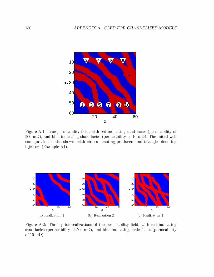
150 APPENDIX A. CLFD FOR CHANNELIZED MODELS
x
y
1
2
3
4
5
6
7
8
9 10
20 40 60
10
20
30
40
50
60
Figure A.1: True permeability field, with red indicating sand facies (permeability of500 mD), and blue indicating shale facies (permeability of 10 mD). The initial wellconfiguration is also shown, with circles denoting producers and triangles denotinginjectors (Example A1).
X
Y
20 40 60
10
20
30
40
50
60
(a) Realization 1
X
Y
20 40 60
10
20
30
40
50
60
(b) Realization 2
X
Y
20 40 60
10
20
30
40
50
60
(c) Realization 3
Figure A.2: Three prior realizations of the permeability field, with red indicatingsand facies (permeability of 500 mD), and blue indicating shale facies (permeabilityof 10 mD).
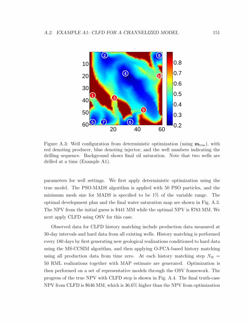
A.2. EXAMPLE A1: CLFD FOR A CHANNELIZED MODEL 151
3000 Days
2
4
5 67
8
1 3
9
10
20 40 60
10
20
30
40
50
60 0.2
0.3
0.4
0.5
0.6
0.7
0.8
Figure A.3: Well configuration from deterministic optimization (using mtrue), withred denoting producer, blue denoting injector, and the well numbers indicating thedrilling sequence. Background shows final oil saturation. Note that two wells aredrilled at a time (Example A1).
parameters for well settings. We first apply deterministic optimization using the
true model. The PSO-MADS algorithm is applied with 50 PSO particles, and the
minimum mesh size for MADS is specified to be 1% of the variable range. The
optimal development plan and the final water saturation map are shown in Fig. A.3.
The NPV from the initial guess is $441 MM while the optimal NPV is $783 MM. We
next apply CLFD using OSV for this case.
Observed data for CLFD history matching include production data measured at
30-day intervals and hard data from all existing wells. History matching is performed
every 180 days by first generating new geological realizations conditioned to hard data
using the MS-CCSIM algorithm, and then applying O-PCA-based history matching
using all production data from time zero. At each history matching step NR =
50 RML realizations together with MAP estimate are generated. Optimization is
then performed on a set of representative models through the OSV framework. The
progress of the true NPV with CLFD step is shown in Fig. A.4. The final truth-case
NPV from CLFD is $646 MM, which is 36.6% higher than the NPV from optimization
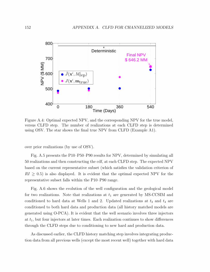
152 APPENDIX A. CLFD FOR CHANNELIZED MODELS
0 180 360 540400
500
600
700
800
Time (Days)
NP
V (
$ M
M)
J(xi,M irep)
J(xi,mtrue)
DeterministicFinal NPV
$ 646.2 MM
Figure A.4: Optimal expected NPV, and the corresponding NPV for the true model,versus CLFD step. The number of realizations at each CLFD step is determinedusing OSV. The star shows the final true NPV from CLFD (Example A1).
over prior realizations (by use of OSV).
Fig. A.5 presents the P10–P50–P90 results for NPV, determined by simulating all
50 realizations and then constructing the cdf, at each CLFD step. The expected NPV
based on the current representative subset (which satisfies the validation criterion of
RI ≥ 0.5) is also displayed. It is evident that the optimal expected NPV for the
representative subset falls within the P10–P90 range.
Fig. A.6 shows the evolution of the well configuration and the geological model
for two realizations. Note that realizations at t1 are generated by MS-CCSIM and
conditioned to hard data at Wells 1 and 2. Updated realizations at t3 and t4 are
conditioned to both hard data and production data (all history matched models are
generated using O-PCA). It is evident that the well scenario involves three injectors
at t1, but four injectors at later times. Each realization continues to show differences
through the CLFD steps due to conditioning to new hard and production data.
As discussed earlier, the CLFD history matching step involves integrating produc-
tion data from all previous wells (except the most recent well) together with hard data
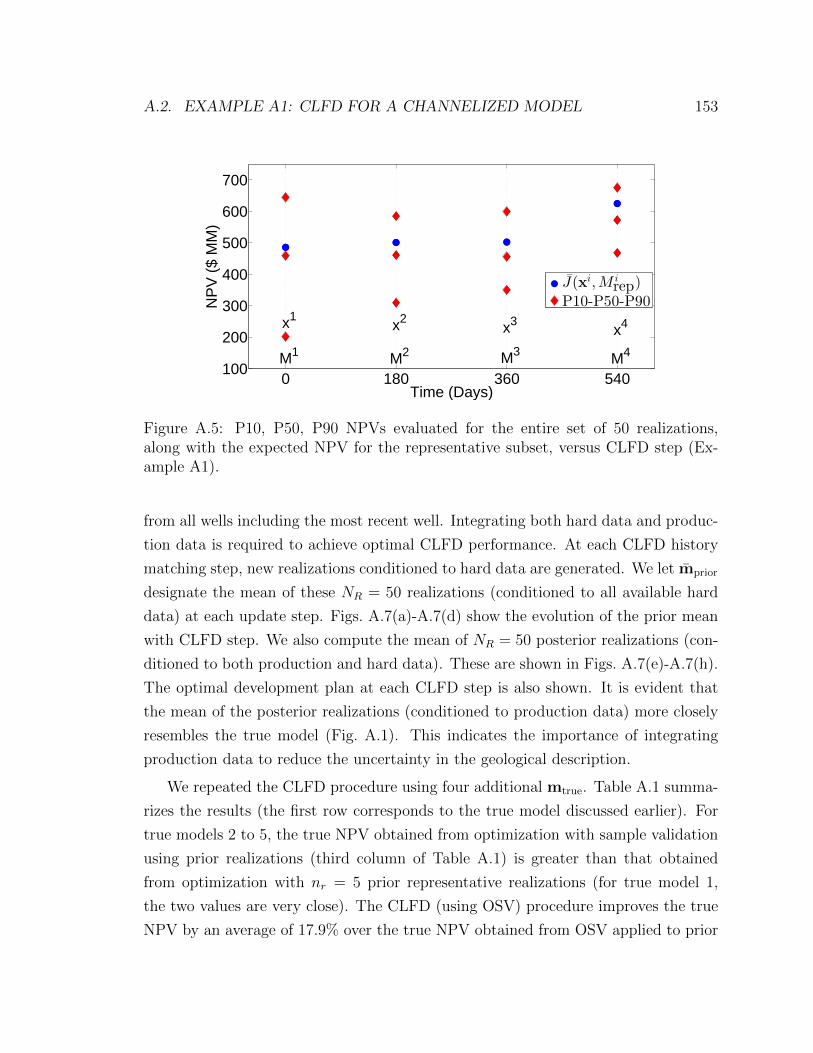
A.2. EXAMPLE A1: CLFD FOR A CHANNELIZED MODEL 153
0 180 360 540100
200
300
400
500
600
700
Time (Days)
NP
V (
$ M
M)
M1
x1
M2
x2
M3
x3
M4
x4
J(xi,M irep)
P10-P50-P90
Figure A.5: P10, P50, P90 NPVs evaluated for the entire set of 50 realizations,along with the expected NPV for the representative subset, versus CLFD step (Ex-ample A1).
from all wells including the most recent well. Integrating both hard data and produc-
tion data is required to achieve optimal CLFD performance. At each CLFD history
matching step, new realizations conditioned to hard data are generated. We let mprior
designate the mean of these NR = 50 realizations (conditioned to all available hard
data) at each update step. Figs. A.7(a)-A.7(d) show the evolution of the prior mean
with CLFD step. We also compute the mean of NR = 50 posterior realizations (con-
ditioned to both production and hard data). These are shown in Figs. A.7(e)-A.7(h).
The optimal development plan at each CLFD step is also shown. It is evident that
the mean of the posterior realizations (conditioned to production data) more closely
resembles the true model (Fig. A.1). This indicates the importance of integrating
production data to reduce the uncertainty in the geological description.
We repeated the CLFD procedure using four additional mtrue. Table A.1 summa-
rizes the results (the first row corresponds to the true model discussed earlier). For
true models 2 to 5, the true NPV obtained from optimization with sample validation
using prior realizations (third column of Table A.1) is greater than that obtained
from optimization with nr = 5 prior representative realizations (for true model 1,
the two values are very close). The CLFD (using OSV) procedure improves the true
NPV by an average of 17.9% over the true NPV obtained from OSV applied to prior
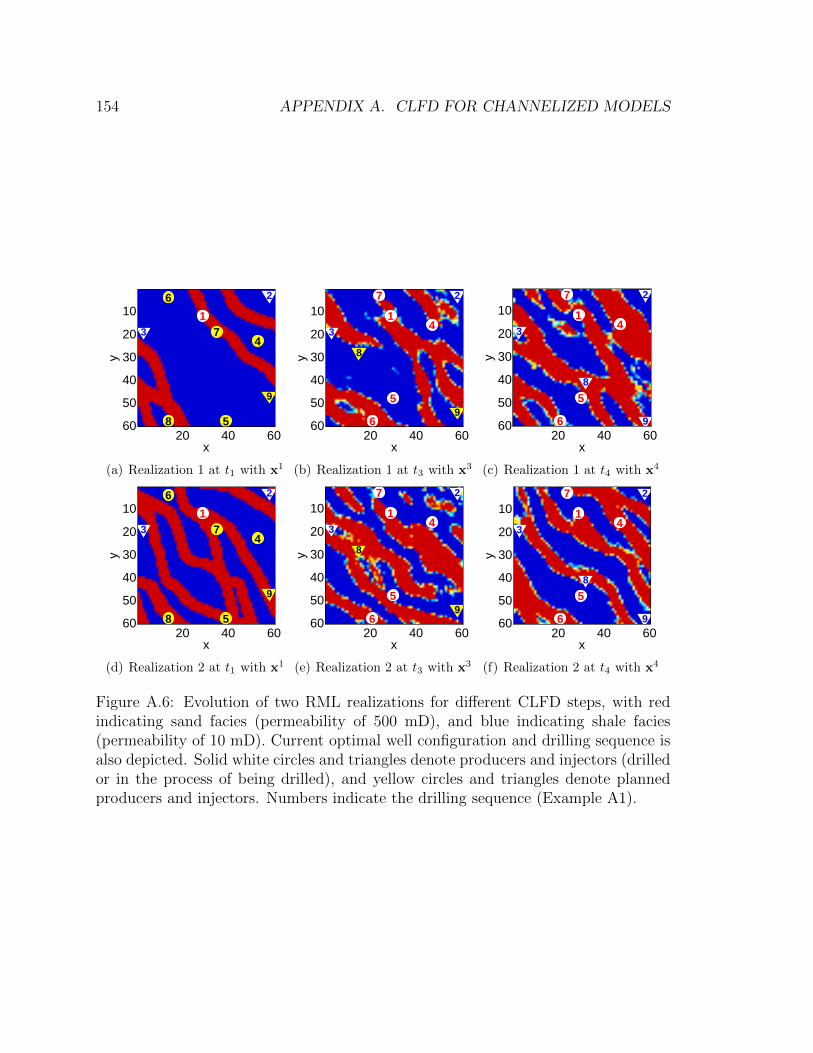
154 APPENDIX A. CLFD FOR CHANNELIZED MODELS
x
y
1
2
34
5
6
7
8
9
20 40 60
10
20
30
40
50
60
(a) Realization 1 at t1 with x1
x
y1
2
34
5
6
7
8
9
20 40 60
10
20
30
40
50
60
(b) Realization 1 at t3 with x3
x
y
1
2
34
5
6
7
8
920 40 60
10
20
30
40
50
60
(c) Realization 1 at t4 with x4
x
y
1
2
34
5
6
7
8
9
20 40 60
10
20
30
40
50
60
(d) Realization 2 at t1 with x1
x
y
1
2
34
5
6
7
8
9
20 40 60
10
20
30
40
50
60
(e) Realization 2 at t3 with x3
x
y
1
2
34
5
6
7
8
920 40 60
10
20
30
40
50
60
(f) Realization 2 at t4 with x4
Figure A.6: Evolution of two RML realizations for different CLFD steps, with redindicating sand facies (permeability of 500 mD), and blue indicating shale facies(permeability of 10 mD). Current optimal well configuration and drilling sequence isalso depicted. Solid white circles and triangles denote producers and injectors (drilledor in the process of being drilled), and yellow circles and triangles denote plannedproducers and injectors. Numbers indicate the drilling sequence (Example A1).
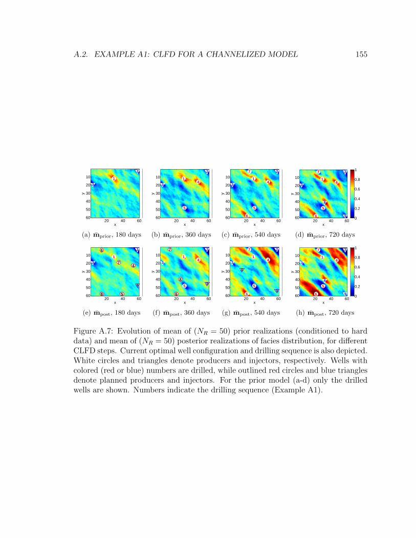
A.2. EXAMPLE A1: CLFD FOR A CHANNELIZED MODEL 155
x
y
1
2
3
20 40 60
10
20
30
40
50
60 0
0.2
0.4
0.6
0.8
1
(a) mprior, 180 days
x
y
1
2
34
5
20 40 60
10
20
30
40
50
60 0
0.2
0.4
0.6
0.8
1
(b) mprior, 360 days
xy
1
2
34
5
6
7
20 40 60
10
20
30
40
50
60 0
0.2
0.4
0.6
0.8
1
(c) mprior, 540 days
x
y
1
2
34
5
6
7
8
920 40 60
10
20
30
40
50
60 0
0.2
0.4
0.6
0.8
1
(d) mprior, 720 days
x
y
1
2
34
5
6
7
8
9
20 40 60
10
20
30
40
50
60 0
0.2
0.4
0.6
0.8
(e) mpost, 180 days
x
y
1
2
34
5
6
7
89
20 40 60
10
20
30
40
50
60
0.2
0.4
0.6
0.8
(f) mpost, 360 days
x
y
1
2
34
5
6
7
8
9
20 40 60
10
20
30
40
50
60 0
0.2
0.4
0.6
0.8
1
(g) mpost, 540 days
x
y
1
2
34
5
6
7
8
920 40 60
10
20
30
40
50
60 0
0.2
0.4
0.6
0.8
1
(h) mpost, 720 days
Figure A.7: Evolution of mean of (NR = 50) prior realizations (conditioned to harddata) and mean of (NR = 50) posterior realizations of facies distribution, for differentCLFD steps. Current optimal well configuration and drilling sequence is also depicted.White circles and triangles denote producers and injectors, respectively. Wells withcolored (red or blue) numbers are drilled, while outlined red circles and blue trianglesdenote planned producers and injectors. For the prior model (a-d) only the drilledwells are shown. Numbers indicate the drilling sequence (Example A1).
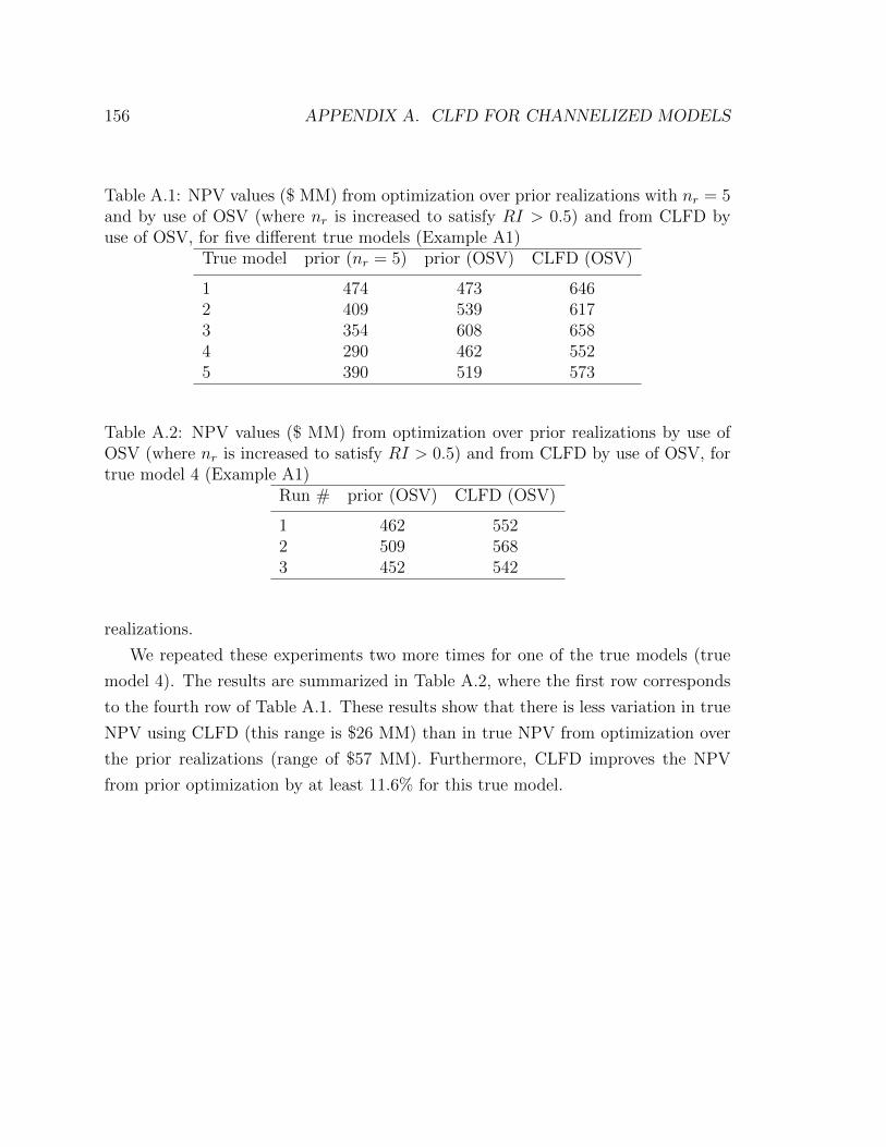
156 APPENDIX A. CLFD FOR CHANNELIZED MODELS
Table A.1: NPV values ($ MM) from optimization over prior realizations with nr = 5and by use of OSV (where nr is increased to satisfy RI > 0.5) and from CLFD byuse of OSV, for five different true models (Example A1)
True model prior (nr = 5) prior (OSV) CLFD (OSV)
1 474 473 6462 409 539 6173 354 608 6584 290 462 5525 390 519 573
Table A.2: NPV values ($ MM) from optimization over prior realizations by use ofOSV (where nr is increased to satisfy RI > 0.5) and from CLFD by use of OSV, fortrue model 4 (Example A1)
Run # prior (OSV) CLFD (OSV)
1 462 5522 509 5683 452 542
realizations.
We repeated these experiments two more times for one of the true models (true
model 4). The results are summarized in Table A.2, where the first row corresponds
to the fourth row of Table A.1. These results show that there is less variation in true
NPV using CLFD (this range is $26 MM) than in true NPV from optimization over
the prior realizations (range of $57 MM). Furthermore, CLFD improves the NPV
from prior optimization by at least 11.6% for this true model.

Appendix B
Representative Realizations for a
Binary System
In this Appendix, the various procedures for selecting representative realizations, pre-
sented in Chapter 3, are applied to a binary channelized reservoir model (recall that,
in Chapter 3, bimodal realizations were considered). In the results presented here,
flow-based features for clustering are computed based on full-physics flow simulations
only; proxy-type tracer flow is not considered.
B.1 Example B1: new well settings
We repeat the numerical experiments presented in Section 3.3 for a set of binary
channelized realizations. The model is two-dimensional and is defined on a 60 ×60 grid. The (isotropic) permeability field, consisting of 3600 grid-block values, is
uncertain. Porosity is specified to be uniform and equal to 0.2. A binary channelized
training image, taken from Vo [138], is considered to provide the facies description. A
set of realizations is then generated using the MS-CCSIM geostatistical method [131].
These realizations are not conditioned to any hard data. The permeability values for
sand and non-sand (shale/mud) facies are 500 mD and 10 mD, respectively. Three
permeability realizations are shown in Fig. B.1. There are six producers and three
injectors in the reservoir (as shown in Fig. B.1). Other simulation parameters are
identical to those in Section 3.3.
157

158 APPENDIX B. REPRESENTATIVE MODELS FOR A BINARY SYSTEM
x
y
1 2 3
4 5 6
7 8 9
20 40 60
10
20
30
40
50
60
(a) Realization 1
xy
1 2 3
4 5 6
7 8 9
20 40 60
10
20
30
40
50
60
(b) Realization 2
x
y
1 2 3
4 5 6
7 8 9
20 40 60
10
20
30
40
50
60
(c) Realization 3
Figure B.1: Three unconditional realizations of binary channelized model. Red indi-cates sand facies (permeability of 500 mD) while blue shows non-sand facies (perme-ability of 10 mD). Fixed well configuration is also shown – circles denote producersand triangles indicate injectors (Example B1).
The reservoir life is 3500 days, which is divided into nt = 7 equal time intervals
(of length 500 days) in the construction of the flow-response vectors. With nine wells
in the model and ncs = 7 control steps, the number of control variables (and the
dimension of the well-parameter vector) is 63. The producer BHP range is 1000–
4100 psi and the injector BHP range is 4600–7000 psi.
B.1.1 Representative realizations for random well controls
The base control strategy for computing flow-based features corresponds to producer
BHPs at their lower bound (1000 psi) and injector BHPs at their upper bound
(7000 psi). The number of flow-based features used in the clustering is 105, which
is equal to the dimension of flow-response vector. For computing the permeability-
based features, each binary realization is represented by l = 70 PCA parameters
(which corresponds to 65% of the total variation).
A total of 300 random well-control vectors (xnew) are generated. BHPs for the
three injectors, from one of the xnew vectors, are shown in Fig. B.2. The flow-response
vectors for all NR = 200 realizations are evaluated and saved for each xnew. This
involves a total of 60,000 simulation runs, which are performed using distributed
computing with access to 200 compute nodes.
Box plots of D for nr = 3 and nr = 6 are shown in Fig. B.3. These results indicate
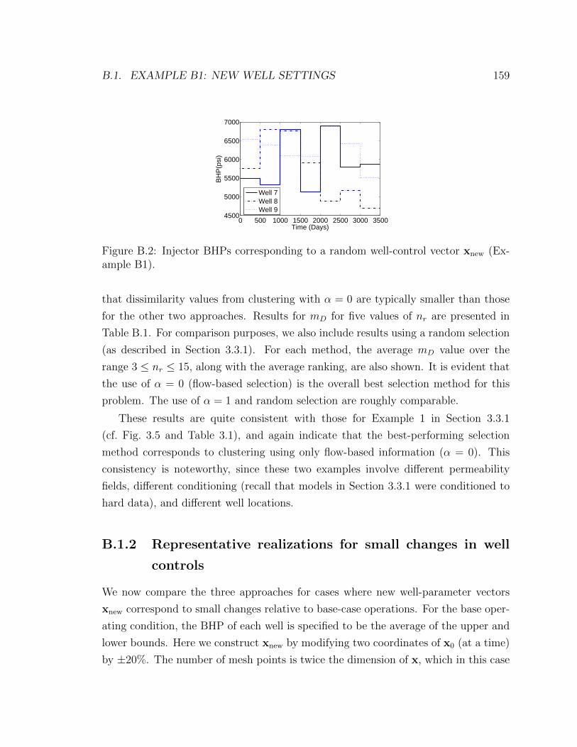
B.1. EXAMPLE B1: NEW WELL SETTINGS 159
0 500 1000 1500 2000 2500 3000 35004500
5000
5500
6000
6500
7000
Time (Days)B
HP
(psi
)
Well 7Well 8Well 9
Figure B.2: Injector BHPs corresponding to a random well-control vector xnew (Ex-ample B1).
that dissimilarity values from clustering with α = 0 are typically smaller than those
for the other two approaches. Results for mD for five values of nr are presented in
Table B.1. For comparison purposes, we also include results using a random selection
(as described in Section 3.3.1). For each method, the average mD value over the
range 3 ≤ nr ≤ 15, along with the average ranking, are also shown. It is evident that
the use of α = 0 (flow-based selection) is the overall best selection method for this
problem. The use of α = 1 and random selection are roughly comparable.
These results are quite consistent with those for Example 1 in Section 3.3.1
(cf. Fig. 3.5 and Table 3.1), and again indicate that the best-performing selection
method corresponds to clustering using only flow-based information (α = 0). This
consistency is noteworthy, since these two examples involve different permeability
fields, different conditioning (recall that models in Section 3.3.1 were conditioned to
hard data), and different well locations.
B.1.2 Representative realizations for small changes in well
controls
We now compare the three approaches for cases where new well-parameter vectors
xnew correspond to small changes relative to base-case operations. For the base oper-
ating condition, the BHP of each well is specified to be the average of the upper and
lower bounds. Here we construct xnew by modifying two coordinates of x0 (at a time)
by ±20%. The number of mesh points is twice the dimension of x, which in this case
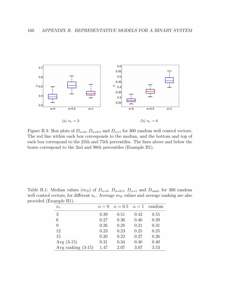
160 APPENDIX B. REPRESENTATIVE MODELS FOR A BINARY SYSTEM
0.3
0.4
0.5
0.6
0.7
α=0 α=0.5 α=1
D
(a) nr = 3
0.25
0.3
0.35
0.4
0.45
0.5
0.55
0.6
α=0 α=0.5 α=1
D
(b) nr = 6
Figure B.3: Box plots of Dα=0, Dα=0.5 and Dα=1 for 300 random well control vectors.The red line within each box corresponds to the median, and the bottom and top ofeach box correspond to the 25th and 75th percentiles. The lines above and below theboxes correspond to the 2nd and 98th percentiles (Example B1).
Table B.1: Median values (mD) of Dα=0, Dα=0.5, Dα=1 and Drand, for 300 randomwell control vectors, for different nr. Average mD values and average ranking are alsoprovided (Example B1).
nr α = 0 α = 0.5 α = 1 random
3 0.39 0.51 0.42 0.556 0.27 0.36 0.46 0.399 0.26 0.28 0.21 0.3112 0.23 0.23 0.25 0.2515 0.20 0.22 0.27 0.26Avg (3-15) 0.31 0.34 0.40 0.40Avg ranking (3-15) 1.47 2.07 3.07 3.53
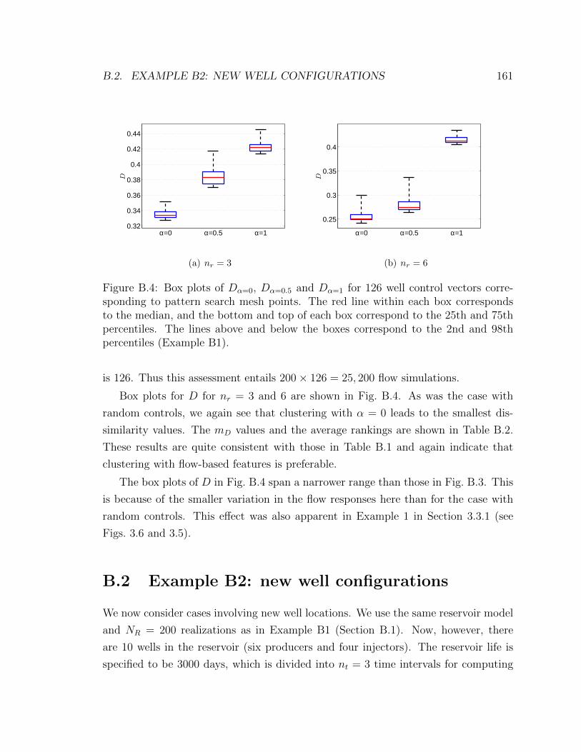
B.2. EXAMPLE B2: NEW WELL CONFIGURATIONS 161
0.32
0.34
0.36
0.38
0.4
0.42
0.44
α=0 α=0.5 α=1
D
(a) nr = 3
0.25
0.3
0.35
0.4
α=0 α=0.5 α=1
D
(b) nr = 6
Figure B.4: Box plots of Dα=0, Dα=0.5 and Dα=1 for 126 well control vectors corre-sponding to pattern search mesh points. The red line within each box correspondsto the median, and the bottom and top of each box correspond to the 25th and 75thpercentiles. The lines above and below the boxes correspond to the 2nd and 98thpercentiles (Example B1).
is 126. Thus this assessment entails 200× 126 = 25, 200 flow simulations.
Box plots for D for nr = 3 and 6 are shown in Fig. B.4. As was the case with
random controls, we again see that clustering with α = 0 leads to the smallest dis-
similarity values. The mD values and the average rankings are shown in Table B.2.
These results are quite consistent with those in Table B.1 and again indicate that
clustering with flow-based features is preferable.
The box plots of D in Fig. B.4 span a narrower range than those in Fig. B.3. This
is because of the smaller variation in the flow responses here than for the case with
random controls. This effect was also apparent in Example 1 in Section 3.3.1 (see
Figs. 3.6 and 3.5).
B.2 Example B2: new well configurations
We now consider cases involving new well locations. We use the same reservoir model
and NR = 200 realizations as in Example B1 (Section B.1). Now, however, there
are 10 wells in the reservoir (six producers and four injectors). The reservoir life is
specified to be 3000 days, which is divided into nt = 3 time intervals for computing
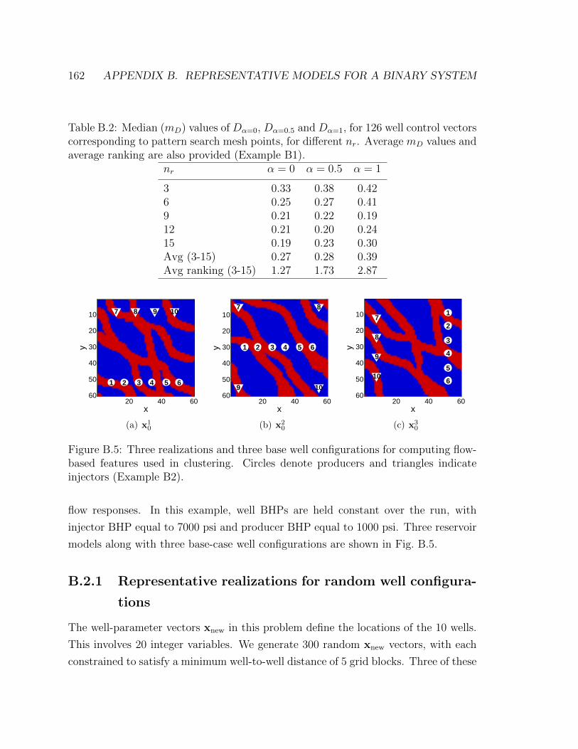
162 APPENDIX B. REPRESENTATIVE MODELS FOR A BINARY SYSTEM
Table B.2: Median (mD) values of Dα=0, Dα=0.5 and Dα=1, for 126 well control vectorscorresponding to pattern search mesh points, for different nr. Average mD values andaverage ranking are also provided (Example B1).
nr α = 0 α = 0.5 α = 1
3 0.33 0.38 0.426 0.25 0.27 0.419 0.21 0.22 0.1912 0.21 0.20 0.2415 0.19 0.23 0.30Avg (3-15) 0.27 0.28 0.39Avg ranking (3-15) 1.27 1.73 2.87
x
y
1 2 3 4 5 6
7 8 9 10
20 40 60
10
20
30
40
50
60
(a) x10
x
y 1 2 3 4 5 6
7 8
9 10
20 40 60
10
20
30
40
50
60
(b) x20
x
y
1
2
3
4
5
6
7
8
9
10
20 40 60
10
20
30
40
50
60
(c) x30
Figure B.5: Three realizations and three base well configurations for computing flow-based features used in clustering. Circles denote producers and triangles indicateinjectors (Example B2).
flow responses. In this example, well BHPs are held constant over the run, with
injector BHP equal to 7000 psi and producer BHP equal to 1000 psi. Three reservoir
models along with three base-case well configurations are shown in Fig. B.5.
B.2.1 Representative realizations for random well configura-
tions
The well-parameter vectors xnew in this problem define the locations of the 10 wells.
This involves 20 integer variables. We generate 300 random xnew vectors, with each
constrained to satisfy a minimum well-to-well distance of 5 grid blocks. Three of these
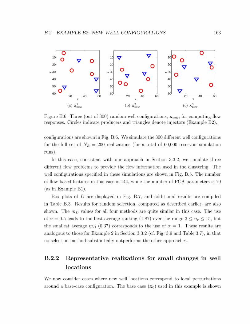
B.2. EXAMPLE B2: NEW WELL CONFIGURATIONS 163
x
y
20 40 60
10
20
30
40
50
60
(a) x1new
x
y
20 40 60
10
20
30
40
50
60
(b) x2new
x
y
20 40 60
10
20
30
40
50
60
(c) x3new
Figure B.6: Three (out of 300) random well configurations, xnew, for computing flowresponses. Circles indicate producers and triangles denote injectors (Example B2).
configurations are shown in Fig. B.6. We simulate the 300 different well configurations
for the full set of NR = 200 realizations (for a total of 60,000 reservoir simulation
runs).
In this case, consistent with our approach in Section 3.3.2, we simulate three
different flow problems to provide the flow information used in the clustering. The
well configurations specified in these simulations are shown in Fig. B.5. The number
of flow-based features in this case is 144, while the number of PCA parameters is 70
(as in Example B1).
Box plots of D are displayed in Fig. B.7, and additional results are compiled
in Table B.3. Results for random selection, computed as described earlier, are also
shown. The mD values for all four methods are quite similar in this case. The use
of α = 0.5 leads to the best average ranking (1.87) over the range 3 ≤ nr ≤ 15, but
the smallest average mD (0.37) corresponds to the use of α = 1. These results are
analogous to those for Example 2 in Section 3.3.2 (cf. Fig. 3.9 and Table 3.7), in that
no selection method substantially outperforms the other approaches.
B.2.2 Representative realizations for small changes in well
locations
We now consider cases where new well locations correspond to local perturbations
around a base-case configuration. The base case (x0) used in this example is shown
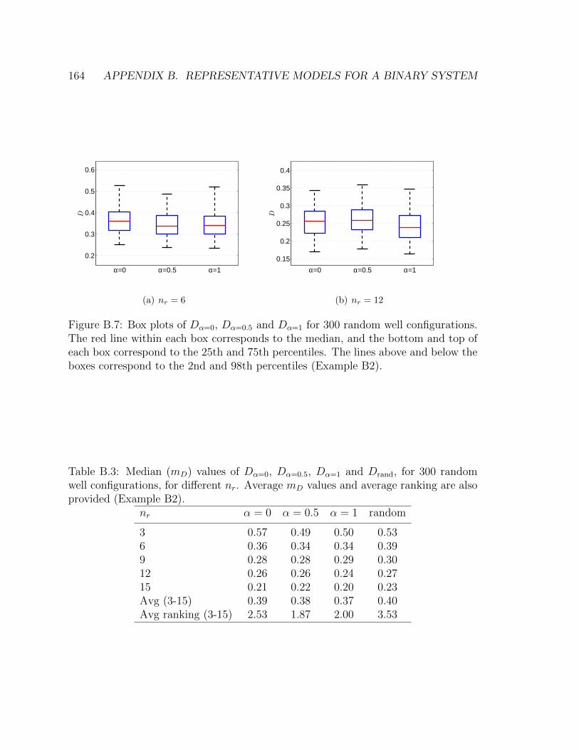
164 APPENDIX B. REPRESENTATIVE MODELS FOR A BINARY SYSTEM
0.2
0.3
0.4
0.5
0.6
α=0 α=0.5 α=1
D
(a) nr = 6
0.15
0.2
0.25
0.3
0.35
0.4
α=0 α=0.5 α=1D
(b) nr = 12
Figure B.7: Box plots of Dα=0, Dα=0.5 and Dα=1 for 300 random well configurations.The red line within each box corresponds to the median, and the bottom and top ofeach box correspond to the 25th and 75th percentiles. The lines above and below theboxes correspond to the 2nd and 98th percentiles (Example B2).
Table B.3: Median (mD) values of Dα=0, Dα=0.5, Dα=1 and Drand, for 300 randomwell configurations, for different nr. Average mD values and average ranking are alsoprovided (Example B2).
nr α = 0 α = 0.5 α = 1 random
3 0.57 0.49 0.50 0.536 0.36 0.34 0.34 0.399 0.28 0.28 0.29 0.3012 0.26 0.26 0.24 0.2715 0.21 0.22 0.20 0.23Avg (3-15) 0.39 0.38 0.37 0.40Avg ranking (3-15) 2.53 1.87 2.00 3.53
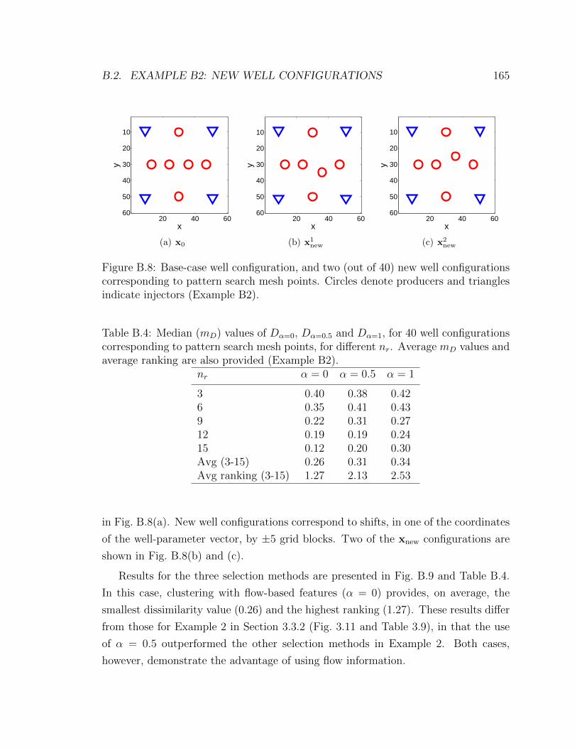
B.2. EXAMPLE B2: NEW WELL CONFIGURATIONS 165
x
y
20 40 60
10
20
30
40
50
60
(a) x0
x
y
20 40 60
10
20
30
40
50
60
(b) x1new
x
y
20 40 60
10
20
30
40
50
60
(c) x2new
Figure B.8: Base-case well configuration, and two (out of 40) new well configurationscorresponding to pattern search mesh points. Circles denote producers and trianglesindicate injectors (Example B2).
Table B.4: Median (mD) values of Dα=0, Dα=0.5 and Dα=1, for 40 well configurationscorresponding to pattern search mesh points, for different nr. Average mD values andaverage ranking are also provided (Example B2).
nr α = 0 α = 0.5 α = 1
3 0.40 0.38 0.426 0.35 0.41 0.439 0.22 0.31 0.2712 0.19 0.19 0.2415 0.12 0.20 0.30Avg (3-15) 0.26 0.31 0.34Avg ranking (3-15) 1.27 2.13 2.53
in Fig. B.8(a). New well configurations correspond to shifts, in one of the coordinates
of the well-parameter vector, by ±5 grid blocks. Two of the xnew configurations are
shown in Fig. B.8(b) and (c).
Results for the three selection methods are presented in Fig. B.9 and Table B.4.
In this case, clustering with flow-based features (α = 0) provides, on average, the
smallest dissimilarity value (0.26) and the highest ranking (1.27). These results differ
from those for Example 2 in Section 3.3.2 (Fig. 3.11 and Table 3.9), in that the use
of α = 0.5 outperformed the other selection methods in Example 2. Both cases,
however, demonstrate the advantage of using flow information.

166 APPENDIX B. REPRESENTATIVE MODELS FOR A BINARY SYSTEM
0.3
0.35
0.4
0.45
0.5
0.55
α=0 α=0.5 α=1
D
(a) nr = 6
0.15
0.2
0.25
0.3
α=0 α=0.5 α=1
D
(b) nr = 12
Figure B.9: Box plots of Dα=0, Dα=0.5 and Dα=1 for 40 well configurations corre-sponding to pattern search mesh points. The red line within each box correspondsto the median, and the bottom and top of each box correspond to the 25th and 75thpercentiles. The lines above and below the boxes correspond to the 2nd and 98thpercentiles (Example B2).
Table B.5: Summary of results: average mD values for nr = 3, . . . , 15 for all cases.The smallest value for each case is indicated in bold.
Case α = 0 α = 0.5 α = 1
Random controls (Ex. B1) 0.31 0.34 0.40PS mesh controls (Ex. B1) 0.27 0.28 0.39Random configs. (Ex. B2) 0.39 0.38 0.37PS mesh configs. (Ex. B2) 0.26 0.31 0.34
B.2.3 Summary of realization-selection results
Table B.5 provides a summary of the results, in terms of the average mD values,
for the four cases considered in this Appendix. For both cases involving new well
controls (either random or pattern-search shifts relative to the base case), the best
performing method for selecting a representative subset was clustering with flow-based
features (α = 0). For randomly-generated new well configurations, the three selection
methods performed similarly, though selection with permeability-based features (α =
1) provided slightly better results than the other approaches. Finally, for small well-
location changes relative to a base well configuration, realizations selected using α = 0

B.2. EXAMPLE B2: NEW WELL CONFIGURATIONS 167
provided the best results. These observations are consistent with those for the bimodal
systems considered in Chapter 3, with the exception that α = 0.5 provided the best
results for small changes in well locations in Chapter 3, while the best results here
are achieved using α = 0.