Add-on Policies under Vertical Differentiation:

Why Do Luxury Hotels Charge for Internet

Whereas Economy Hotels Do Not?

Song Lin

Hong Kong University of Science and Technology

June 2015

Abstract

This paper examines firms’ product policies when they sell an add-on (Internet

service) to a base good (hotel rooms) under vertical differentiation (four- vs. three-star

hotels). Theoretical analysis uncovers the differential roles of add-ons for vertically

differentiated firms. A firm with higher base quality always sells an add-on as optional

so that higher-taste consumers self-select to buy it. This incentive to price discriminate

applies to a lower-quality firm who, however, has to lower the add-on price to lure

consumers considering the higher-quality base good without the add-on. If providing

the add-on is not costly, the lower-quality firm may sell it as standard. This equilibrium

potentially explains the puzzle that lower-end hotels are more likely than higher-end

ones to offer free Internet service. Empirical examination of a sample of hotels that

are likely to be in a monopoly or vertical duopoly market provides suggestive evidence

for this prediction.

Surprisingly, an optional add-on can intensify competition, in contrast to standard

conclusions in the literature. If both firms sell an optional add-on, they will price

aggressively to compete for consumers who trade off the higher-quality base versus the

lower-quality base good plus the add-on. Although selling the add-on as optional is

unilaterally optimal, equilibrium profits may reduce - a Prisoner’s Dilemma outcome.

1 Introduction

Although Internet service is a necessity and is available in most hotels, only 54% of luxury

hotels provide it for free. In contrast, the percentage grows to 72%, 81%, 93%, and 91% for

upscale, mid-priced, economy, and budget hotels, respectively.1 This phenomenon appears

to be counter-intuitive, attracting considerable public attention and media coverage.2 Why

does the phenomenon persist? The answer to the question may have important managerial

implications. In many industries, it is common for firms to sell a base good or service as their

primary business, and then sell a complementary item or upgrade (hereafter, “add-on”).3

Examples include airlines selling drinks and snacks on a flight, car manufacturers selling

upgrades such as GPS and leather seats on top of a base model, and mobile applications

offering in-app purchases or premium upgrades. Solving the puzzle elucidates what product

policies firms should adopt: Should they sell an add-on separately from the base good as

optional, sell it as standard (i.e., free), or not sell it at all?

Existing pricing theories do not offer adequate explanations to this puzzle. Conventional

wisdom from monopoly pricing suggests that selling an add-on as optional allows a firm with

market power to price discriminate to enhance profit. This argument, however, contradicts

the practice of lower-end hotels. A simple explanation would be that consumers staying

at higher-end hotels are less price-sensitive.4 However, this argument would suggest that

1The phenomenon also applies to other hotel amenities such as breakfast and local phone calls. The datasource is 2012 Lodging Survey by American Hotel & Lodging Association. In the empirical section I providedetails of the survey data.

2 To name a few: “The price of staying connected” (New York Times, 5/6/2009), “Hotel guests cravefree Wi-Fi” (Los Angeles Times, 9/6/2010), “Luxury hotels free up Wi-Fi” (Wall Street Journal, 5/5/2011),“Wi-Fi in hotels: the most unkindest charge of all” (The Economist, 5/16/2011), “Some hotels with freeWi-Fi consider charging for it” (USA Today, 6/22/2012), “Wi-Fi fees drag hotel satisfaction down” (CNN,7/25/2012).

3 Some add-ons are better described as surcharges, which are mandatory or necessary after the purchaseof a base good. Examples include taxes for most services and goods, fuel surcharges for airlines, concessionrecovery fees for car rental at airport locations, etc. A recent stream of behavioral research on partitionedpricing explores how consumers react under this situation (e.g., Morwitz et al. 1998, Cheema 2008). Thispaper restricts attention to add-ons that are not mandatory or not necessary on the purchase of a base good.

4 There are several related explanations along the same line. For example, one may argue that consumers

1

the higher-end hotels charge a higher total price rather than separate Internet charges from

room rates. Shugan and Kumar (2014) compare the hotel industry to the airline industry

and argue that it is optimal for a monopolist with a product line of base services to bundle

add-ons with its lower-end base to decrease the base differentiation when the differentiation

is large (hotel industry), and to unbundle add-ons with its lower-end base when the base

differentiation is small (airline industry). However, this theory does not explain why the

phenomenon persists even when higher-end and lower-end hotels are not owned by the same

company, and why policies are different for different types of add-ons within an industry (e.g.,

mini-bar, laundry, or airport shuttle services in the hotel industry). I propose a different

but complementary explanation that vertical differentiation between competing firms plays a

role. I develop a competitive theory of add-on pricing to examine how vertical differentiation

can lead to a divergence in product policy. The theory leads to three interesting insights.

First, the theory identifies the differential roles of add-ons for vertically differentiated

firms. A firm with higher base quality behaves more or less like a monopolist. Selling an

add-on as optional at a high price serves as a screening or segmentation device so consumers

with higher tastes for quality self-select to buy the expensive add-on. This incentive to

screen consumers also applies to a firm with lower base quality. However, the lower-quality

firm is incentivized to lower the add-on price to lure those consumers, who may consider

buying the higher-quality base without paying for the add-on, to switch to the lower-quality

base with the add-on. This vertical differentiation role of the add-on is absent from extant

literature on add-on pricing, which focuses on unobserved add-on prices with horizontal or

no differentiation (Lal and Matutes 1994, Verboven 1999, Ellison 2005, Gabaix and Laibson

2006).5 Due to the trade-off between screening and differentiation, the lower-quality firm’s

at higher-end hotels have corporate accounts covering their expenses whereas consumers at lower-end hotelstravel with their own accounts. Another related argument is that higher-end hotels customers are typicallybusiness travelers whereas lower-end hotels have more leisure travelers.

5 The term “add-on pricing” has been used to refer to a specific situation with unobserved add-on prices(Ellison 2005). In this paper the term refers to broader problems that involve pricing of a base good and an

2

policy is sensitive to the efficiency of supplying the add-on. The firm will not sell the add-on

if it is too costly to provide the add-on to improve quality because it has to charge a high

add-on price that discourages consumers from buying (e.g., mini-bar). In equilibrium, the

lower-quality firm sell the add-on only if it is not too costly. If the cost becomes sufficiently

small (e.g., Internet service), the add-on price will be so low that all consumers who buy

the base from the lower-quality firm will also pay for the add-on. Consequently, the higher-

quality firm will sell the add-on as optional, whereas the lower-quality firm will sell it as

standard. This equilibrium outcome provides one possible explanation of the stylized fact.

Examining a sample of monopoly and duopoly markets with vertical differentiation in

the American hotel industry, I find suggestive evidence for the theoretical predictions when

the cost of an add-on is very small (i.e., Internet service). On the one hand, a hotel at the

higher end of a vertical duopoly market is as likely as a monopoly hotel to charge for Internet

service, consistent with the theory that higher-quality firms focus on screening consumers,

behaving like a monopolist. On the other hand, a hotel is more likely to offer free Internet

service if it is at the lower end of a vertical duopoly market. This finding supports the

theory that vertical differentiation introduces a trade-off for lower-quality firms, which find

it optimal to sell an add-on as standard rather than sell it as optional. Conclusions are

robust even after controlling for a number of potentially confounding factors such as hotel

segment, location, size, age, operation, etc.

Second, the theory leads to a surprising prediction that selling an add-on as optional

intensifies competition. Since a higher-quality firm sells an add-on to its higher-taste con-

sumers, leaving some lower-taste consumers who do not buy the add-on, it creates an oppor-

tunity for a lower-quality firm to lower its add-on price to induce switching. The firms then

price aggressively to compete for these marginal consumers who trade off the higher-quality

base good versus the lower-quality base good including the add-on. Although the optional-

add-on, regardless of the observability of the add-on price.

3

add-on policy is unilaterally optimal, a Prisoner’s Dilemma emerges in which both firms

lose profits in equilibrium. The result is striking. Extant literature predicts that selling an

add-on as optional either has no impact on firm profits under competition (Lal and Matutes

1994), or softens price competition (Ellison 2005). The profit-irrelevant result is based on the

argument that any profit earned from selling a high-priced add-on is competed away on the

base price. The competition-softening result hinges on the idea that with the add-on prices

unobserved naturally, firms create an adverse selection problem that makes price-cutting un-

appealing, thereby raising equilibrium profits. In contrast, I identify a mechanism by which

selling an add-on hurts firm profits. The mechanism does not rely on the unobservability

of add-on prices. It is the interaction between the screening effect and the differentiation

effect that reverses standard conclusions on the profitability of selling an add-on. Due to the

intensified competition, the higher-quality firm may want to commit to a standard-add-on

policy, and the lower-quality firm to commit to a no-add-on policy, if such commitments

are possible. Luxury cars, for example, are more likely than economy cars to offer some

advanced features such as standard leather seats, GPS navigation, side airbags, etc.

Third, when consumers do not observe add-on prices, hold-up problems arise naturally.

However, unlike other settings in the literature, vertical differentiation moderates the effects

of hold-up on firm profits in this context. The higher-quality firm’s policy is unaffected by

the unobservability of the add-on price, because its consumers already expect the add-on

to be expensive due to the firm’s screening incentive. The hold-up effect coincides with the

screening effect for the higher-quality firm. Anticipating being held up by the lower-quality

firm, some consumers refrain from buying from it and switch to the higher-quality base good

without paying for the add-on. Consequently, the higher-quality firm demands a higher base

price, but the lower-quality firm is forced to lower its base price while keeping the add-on

price high. In equilibrium the higher-quality firm is better off, whereas the lower-quality firm

is worse off, suggesting that the higher-quality firm has no incentive to advertise the add-on

4

price, whereas the lower-quality firm has a strict incentive to advertise. This prediction

contrasts sharply with extant results that a hold-up problem has no impact on firm profits

under competition because profits earned by holding up consumers ex post are competed

away by lowering base prices (i.e., “loss leader”; Lal and Matutes 1994).

Related Literature

This study relates to broader literature on price discrimination and multi-product pricing.

Not surprisingly, add-on pricing can be a form of second-degree price discrimination. A base

good including an add-on versus the base good alone can be viewed as two quality levels.

If firms sell an add-on as standard, they essentially sell the same quality to all consumers

with no price discrimination. If firms instead adopt an optional-add-on policy, they sell

the bundle (i.e., the higher-quality level) to consumers with higher tastes for quality while

selling only the base (i.e., the lower-quality level) to lower-taste consumers. In monopoly

markets, it is generally optimal for firms to price discriminate. The problem is much harder

to analyze under imperfect competition. Extant studies of competitive second-degree price

discrimination (Stole 1995, Armstrong and Vickers 2001, Rochet and Stole 2002, Ellison

2005, Schmidt-Mohr and Villas-Boas 2008) examine settings in which firms are symmetric,

finding that firms engage in price discrimination if sufficient consumer heterogeneity exists.

They do not consider the possibility of vertical pressure competing firms face, a scenario

that arises often in the real world. One exception is Champsaur and Rochet (1989), who

study differentiated firms in a duopoly market competing by offering ranges of quality to

heterogeneous consumers. After firms’ investments in quality ranges, they determine the

optimal nonlinear pricing policies. The price-setting game, given differential quality ranges,

is similar in spirit to the pricing game I study here. However, unlike those authors, I study the

context of add-on pricing in which quality is discrete, and derive implications of competitive

price discrimination on profitability.

5

The result that selling an add-on intensifies competition also relates to several findings

in the literature. Although it is generally true that monopolists find it optimal to price dis-

criminate among consumers, this conclusion is no longer robust under competitive settings.

Price discrimination can intensify competition, thereby hurting profits. One mechanism by

which this result arises is competitive third-degree price discrimination (Thisse and Vives

1988, Shaffer and Zhang 1995, Corts 1998). Corts (1998) points out that when firms have

a divergent view on the ranking of consumer segments (i.e., a strong market for one firm is

weak for the other), it is possible that price discrimination leads to lower prices in all market

segments, reducing profits.6 Another mechanism giving rise to this result is competitive

mixed bundling in the two-stop shopping framework (Matutes and Regibeau 1992, Anderson

and Leruth 1993, Armstrong and Vickers 2010).7 Practicing mixed bundling might trigger

fierce price competition, lowering prices for component products. Consequently, profits re-

duce. This paper identifies an alternative mechanism that differs substantially in terms of

modeling framework and business context. The add-on pricing problem studied here differs

from third-degree price discrimination because firms do not know consumers’ preferences,

and thus rely on incentive compatibilities to practice price discrimination. The problem is

also different from multi-product bundling because an add-on is only available and valuable

conditional on the purchase of a base good.8 Nevertheless, the recurring theme underlying

the competition-intensifying result appears to be that competing firms price aggressively to

acquire consumers who trade off between buying a higher-quality level from one firm versus

buying a lower-quality level from another.

Finally, this paper relates to growing academic and industrial interest in drip pricing.9

6 Many cases exist in which this condition does not hold, and thus competing firms are better off inequilibrium (e.g., Chen et al. 2001, Shaffer and Zhang 2002).

7When competing firms offer multiple products, they can either sell the component products alone (i.e.,component pricing), or sell the products in a bundle (i.e., pure bundling), or both (i.e., mixed bundling).

8 Consumers cannot buy the add-on without buying the base good, but they can buy the base good alonewithout buying the add-on. For example, a consumer cannot access Internet service in a hotel if she doesnot stay at the hotel, but she can stay in the hotel room without using the Internet service.

9 The Federal Trade Commission defines drip pricing as “a pricing technique in which firms advertise only

6

The leading theory that explains why firms adopt drip pricing is that it is profitable to exploit

myopic consumers who do not anticipate the hidden cost. Gabaix and Laibson (2006) show

that firms may choose not to advertise add-on prices (i.e., shrouding) even under perfect

competition. Shulman and Geng (2012) extend the mechanism to the situation in which

firms are ex ante different in both horizontal and vertical dimensions. Dahremoller (2013)

introduces a commitment decision of shrouding or unshrouding, which can alter underlying

incentives to unshroud. Muir et al. (2014) provide empirical evidence of drip pricing that

driving schools take advantage of the fact that many students are not aware of extra driving

school fees when they take a base course of driving instruction. Unlike these authors, I

examine long-run market outcomes in which consumers know or correctly anticipate add-on

prices in equilibrium. This assumption is not unreasonable, given that consumers might

learn about prices through repeat purchases and/or word-of-mouth,10 and in many cases,

firms advertise add-on policies because they care about reputation or regulations require

disclosure. It is unlikely that the motivating stylized fact is driven by consumer myopia,

given that repeat purchases are common in the hotel industry and Internet service is a

highly expected and frequently used feature.11 Results from this study suggest that vertical

differentiation not only has profound impacts on add-on policies even under complete price

information, but also interacts with firms’ incentives to advertise add-on prices when they

are unobservable.

part of a product’s price and reveal other charges later as the customer goes through the buying process.The additional charges can be mandatory charges, such as hotel resort fees, or fees for optional upgradesand add-ons.”

10 For example, having stayed at Marriott and learned that Internet service costs $13, a consumer maykeep this in mind the next time she books a room at the same hotel or at another location of the same chain.

11 If consumers are boundedly rational, then Internet fees should be shrouded and higher than marginalcosts at both the luxury and economy hotels.

7

2 A Theory of Add-on Policy under Vertical Differentiation

In this section, I present a theory that explains why and when a divergence in product policy

arises as an equilibrium outcome. I first write down the simplest model that illustrates the key

underlying mechanism, and then relax some of the simplifying assumptions to demonstrate

that they do not alter the main message of the mechanism.

2.1 Model Setup

There are two firms j ∈ {l, h}, that differ in terms of the quality of the base good V such

that Vh > Vl > 0. The quality difference, or quality premium, is ∆V . The marginal cost of

the base good is normalized to zero for both firms. In an extension discussed later, I allow

the marginal cost to be different for the two firms. In addition to the base good, an add-on

technology is available. The add-on has value w and costs c, the same for both firms. Again,

the symmetric assumption is made only to simplify analysis. Qualitative conclusions remain

largely unaffected in an extension with asymmetric add-on considered later. The efficiency

of supplying the add-on is measured by the cost-to-value ratio, α = c/w, which plays an

important role in the equilibrium analysis. It is assumed that the quality premium is greater

than the value of the add-on, ∆V > w, allowing interesting equilibria to arise. Each firm

can set base price Pj and add-on price pj.

A continuum of consumers differ in their marginal valuation, or taste, for quality. The

taste parameter, θ, is distributed uniformly with θ ∈ [θ, θ] and θ > 0.12 Two assumptions

are made throughout the analysis. First, θ > 2θ, so there is a sufficient amount of consumer

heterogeneity in the market. Second, θ > α, so there are positive sales of the add-on in

12 The assumption that the lower bound is positive, combined with a sufficiently large base quality Vj ,ensures that the market is fully covered. It simplifies analysis by focusing on the interaction between thetwo firms, assuming away the outside option of not buying from any firm.

8

equilibrium. The utility of buying from firm j for type-θ consumer is

Uθj =

θVj − Pj if only the base good is purchased;

θ(Vj + w)− Pj − pj if both the base good and the add-on are purchased.

(1)

The base and add-on values V and w are both common knowledge to all parties. This is not

an unreasonable assumption for industries such as the hotel industry in which consumers pos-

sess sufficient knowledge or information due to say repeat purchases.13 However, consumers

know their own tastes θ, but the firms do not. The firms only know the distribution of tastes,

and hence rely on incentive compatibilities to screen consumers or price discriminate.

It is worth noting that the assumption that the unobserved consumer preferences are

summarized entirely in one dimension, θ, may appear strong, but it keeps the model tractable.

An alternative interpretation is that tastes are the inverse of price sensitivities.14 The implicit

restriction behind this setup is that willingness-to-pay for the base good and for the add-

on (θVj and θw) correlate perfectly. Nevertheless, the mechanism does not rely on this

assumption, as shown in an extension with imperfectly correlated tastes in the Appendix.

What is necessary is that there is unobserved heterogeneity in both the base good and add-

on, enabling consumers to trade off between the add-on and the base quality.15 For price

discrimination to arise, the single-crossing property is necessary such that higher tastes for

the value of an add-on and for a base quality imply higher willingness-to-pay for the add-on

13 There are, of course, situations in which consumers experience uncertainty about V and/or w. If firmshave superior knowledge on these values, then the add-on can signal the base quality. For example, Bertiniet al. (2009) show that add-on features can influence consumers’ evaluations of a base good about which theyare uncertain. How firms design product policies under this situation is an interesting direction to explore,but it is beyond the scope of this paper. If firms are also uncertain about these values, insights from thissimpler specification of consumer utility may apply.

14 One can specify an equivalent preference model such that the utility of buying both a base and anadd-on is given by Uθj = Vj + w − (Pj + pj)/θ.

15 This feature distinguishes the paper from Dogan et al. (2010). In their model of competitive second-degree price discrimination with vertical differentiation in the context of rebates, there is no unobservedheterogeneity in tastes for the base quality.

9

and for the higher-quality base.

The strategic interaction is modeled as a full-information simultaneous-move game. Both

firms announce prices simultaneously, (Ph, ph) and (Pl, pl). Consumers observe all prices

and decide which firm to visit and whether to pay for an add-on from the chosen firm.

The formulation naturally builds on two stylized models. If there is no add-on, the model

reduces to a duopoly model of vertical differentiation (Shaked and Sutton 1983). If there is

no competition, the model reduces to a monopoly model of nonlinear pricing (Mussa and

Rosen 1978) with continuous-type consumers and discrete qualities. Each reduced model

is straightforward to solve. However, combining the two features complicates equilibrium

analysis dramatically due to the many possibilities of market outcome. Specifically, each

firm can price its base and add-on to implement any of the following three outcomes, taking

into account consumers’ incentive compatible decisions:

No Add-on: No consumer buys the add-on. All consumers buy just the base good.

Standard Add-on: All consumers buy the add-on. It is essentially bundled with the

base good because only the total or bundle price matters.

Optional Add-on: Some but not all consumers buy the add-on. The higher-type con-

sumers buy it, whereas the lower-type consumers buy only the base.

There are nine possible market configurations, depending on the implementations by both

firms. Each configuration constitutes a possible equilibrium profile. To prove the existence

of an equilibrium for each profile, one has to examine, for each firm, all non-local deviations

that lead to any form of the remaining eight possible market configurations. However, the

solution to the game can be simplified by observing that the higher-quality firm always

serves the highest-type consumers and thus may have a strong incentive to sell the add-on

as optional in equilibrium. The next sub-section formalizes this intuition.

10

2.2 The Higher-quality Firm Focuses on Screening

If the higher-quality firm implements the optional-add-on policy, it essentially divides its pool

of consumers into two segments. The higher-type consumers, θ ∈ [θh, θ], buy both the base

and the add-on. Type θh is the intra-marginal consumer who is indifferent between buying

the bundle and buying only the base, and it is equal to ph/w. The remaining lower-type

consumers, θ ∈ [θhl, θh], buy the base only. This segmentation is a result of the single-crossing

property that higher-type consumers self-select to buy the add-on. Type θhl is the marginal

consumer who is indifferent between buying from the higher-quality or lower-quality firm.

This marginal consumer is only affected by base price Ph, and the add-on price is irrelevant.

The firm’s profit decomposes into two additive profit components

Πh = (θ − θhl)Ph + (θ − θh)(ph − c)︸ ︷︷ ︸πh(ph)

. (2)

The first is the profit from selling the base good, independent from the add-on price since it is

irrelevant to the marginal consumer θhl. The second is the additional profit from selling the

add-on, independent from the base price. Without considering incentive constraint θh ≥ θhl,

to maximize profit, the higher-quality firm simply chooses the appropriate base and add-on

prices to maximize the two components separately. If, however, the incentive constraint is

binding, all consumers will buy the bundle. In this case, the firm is selling the add-on as

standard and a single bundle price P+h suffices. Since the firm serves consumers with the

highest tastes in the market, it relaxes the pressure for a binding constraint. Just as in a

monopoly market, the higher-quality firm can easily find the optional-add-on policy strictly

better than the standard-add-on policy. The following lemma formalizes this observation.

(All proofs are provided in the Online Appendix.)

Lemma 1. For the higher-quality firm, selling the add-on as standard is strictly dominated

11

by selling the add-on as optional, if:

1. Pl > −α∆V when the lower-quality firm does not sell the add-on, or

2. P+l > −α(∆V − w) when the lower-quality firm sells the add-on.

The intuition behind this lemma is simple. When the higher-quality firm sells the add-

on as standard, the add-on price is set sufficiently low so that all of its consumers buy it.

Consider a local deviation whereby the firm increases the add-on price by a small amount ε

and decreases the base price by the same amount. Then some consumers refrain from paying

for the add-on (i.e., the firm implements the optional-add-on policy). On the one hand,

increasing the add-on price does not lose many consumers who have originally bought the

add-on, but it generates additional revenue from those higher-type consumers who continue

to pay for it. On the other hand, lowering the base price expands the market. Acquired

consumers are of the lower types so the loss due to the lower base price is quite limited.

The total profit is then increased. Note that the argument requires that there is sufficient

number of different types (more than two) so that a local deviation by separating the prices

is profitable.16 This intuition is the similar to that in a monopoly market. Despite facing

competitive pressures from the lower-quality firm, the higher-quality firm behaves like a

monopolist. The first main proposition follows.

Proposition 1. In any equilibrium, if it exists, the higher-quality firm sells the add-on as

optional.

The mechanism for the higher-quality firm accords with what many managers have in

mind. One reason luxury hotels charge for Internet service is “because they can”. Selling

optional Internet service is so lucrative that these hotels do not want to give up this source

of revenue. One driving force is the firm’s incentive to screen consumers, an effective way to

16 With just two types of consumers, it can easily lead to the conclusion that selling an add-on as standardis optimal, as in Ellison (2005) and Shugan and Kumar (2014).

12

boost short-term profits. This incentive should also apply to the lower-quality firm, given

that it also serves a pool of consumers with heterogeneous tastes. Why does the lower-quality

firm behave differently? The next sub-section provides the answer.

2.3 The Lower-quality Firm Trades off Screening and Differentiation

Having shown that the only possible implementation of the higher-quality firm is the optional-

add-on policy, there are only three possible equilibrium profiles to be considered, depending

on the lower-quality firm’s implementation. In what follows I develop the equilibrium in

which the lower-quality firm sells the add-on as optional. The other two possible equilibria

become straightforward given this development.

The lower-quality firm now targets consumers of lower types, θ ∈ [θ, θhl]. Similar to

the higher-quality firm, it segments consumers into two groups. The lower-type consumers,

θ ∈ [θ, θl], buy only the base good. The intra-marginal consumer, who is indifferent between

buying the bundle and buying only the base, is given as θl = pl/w. This consumer does not

react to the base price of the higher-quality firm. Consumers of higher types, θ ∈ [θl, θhl], buy

both the base and add-on. The marginal consumer, who is indifferent between the two firms,

θhl, depends on the lower-quality firm’s total price of the base and add-on, P+l = Pl + pl.

The profit is

Πl = (θhl − θ)Pl + (θhl − θl)(pl − c).

Like its rival, the lower-quality firm is incentivized to set a high add-on price to allow the

consumers self-select. Those who have a higher taste for quality consider the high-priced

add-on, and the lower-type consumers consider only the base. Unlike its rival, however, the

lower-quality firm also uses the add-on to attract consumers who consider only the base

from the competitor. The firm attempts to keep its add-on price reasonably low to attract

these potential switchers. To see the optimal pricing strategy that resolves this trade-off, it

13

is instructive to rewrite the firm’s profit as

Πl = (θhl − θ)(P+l − c)−(θl − θ)(pl − c)︸ ︷︷ ︸

πl(pl)

. (3)

In this decomposition, the first component depends only on bundle price P+l , and the second

depends only on add-on price pl. The unconstrained problem is solved by maximizing each

component separately. The intuition can be understood as follows. The lower-quality firm

advertises an attractive bundle package (e.g., a 3-star hotel offers “Internet included” or

“stay-connected” packages) to its potential consumers, θ ∈ [θ, θhl], and convinces all to

visit. Once consumers accept the offer, the firm excludes the lowest-type consumers, θ ∈

[θ, θl], from consuming the add-on by subsidizing them to not consume it. In this way, the

firm attracts its most valuable consumers, θ ∈ [θl, θhl], while avoiding unnecessary costs of

supplying the add-on to the lowest-type consumers, who do not value it much.

The strategic interaction between the two firms reduces to the competition between the

lower-quality firm’s bundle and the higher-quality firm’s base good. They compete for the

marginal consumer who is indifferent between the two, given by θhl = (Ph−P+l )/(∆V −w).

The competition is the same as a duopoly model of vertical differentiation,17 except that the

quality premium is ∆V − w instead of ∆V , and that the lower-quality firm’s price is P+l

instead of Pl. In equilibrium, the prices are

P ∗h =1

3(∆V − w)(2θ − θ) +

1

3c, and P+∗

l =1

3(∆V − w)(θ − 2θ) +

2

3c, (4)

and the marginal consumer is

θ∗hl =1

3(θ + θ)− c

3(∆V − w), (5)

17 See Tirole (1988) for a stylized model.

14

which determines the equilibrium market share of each firm. Note that equilibrium marginal

consumer, θ∗hl, decreases with add-on value w. As the value grows, two opposite effects

occur. On the one hand, there is a direct effect of increasing demand for the lower-quality

firm, and decreasing demand for the higher-quality firm, because consumers obtain higher

utility from the lower-quality firm due to the added value of the add-on. For fixed prices, the

marginal consumer moves upward as w increases. On the other hand, there is an indirect

effect stemming from strategic price responses to changes in product quality. The higher-

quality firm lowers its base price as value w increases. Contrarily, the lower-quality firm

raises its bundle price to exploit acquired consumers who have higher tastes. The price gap

is reduced, moving the marginal consumer downward. In equilibrium, which effect dominates

depends on the cost of the add-on relative to the cost of the quality premium. In the current

setup, the strategic effect dominates given that the cost of the quality premium is small (i.e.,

assumed to be zero), and hence the marginal consumer becomes lower as w increases.18

Independent of strategic interactions that determine equilibrium market shares, the firms

set an optimal add-on price. Add-on prices ph and pl are chosen to maximize πh(ph) and

πl(pl) in Equations (2) and (3) respectively, which lead to

p∗h =1

2(θ + α)w, and p∗l =

1

2(θ + α)w,

with resulting intra-marginal consumers: θ∗h = 12(θ + α) and θ∗l = 1

2(θ + α). The optimal

add-on prices reflect underlying consumer tastes. Although the add-on is the same for both

firms, the price is higher at the higher-quality firm. This accords with the casual observation

that Internet fees at higher-end hotels are higher than those at lower-end hotels (if they

charge for it). Furthermore, the add-on price at the higher-quality firm is higher than the

marginal cost, suggesting that it is a profitable business. However, the price is considerably

18 In the extension in which the marginal cost of the base good is asymmetric, this conclusion holds aslong as the cost of the add-on is greater than the cost of the quality premium.

15

lower at the lower-quality firm, even lower than the marginal cost. In fact, the lower-quality

firm prices the add-on significantly lower than what it would have charged if there were no

competition. To see that, imagine that the lower-quality firm is the monopolist for a market

of consumers with types θ ∈ [θ, θl]. The maximization problem would lead to an add-on price

of p∗l = 12(θl + α)w, which is greater than p∗l in the equilibrium under vertical differentiation

because θl > θ. This is true even though θl can be much smaller than θ. The fact that the

lower-quality firm serves the consumers with lower tastes is not the main driver of the low

add-on price; vertical differentiation forces the firm to price it considerably low, even below

the marginal cost.

2.4 Incentive Compatibility and Equilibrium Outcomes

The preceding analysis uncovers the equilibrium pricing under the scenario in which both

firms sell the add-on as optional. This equilibrium exists as long as the following incentive

constraints hold:

(1) θ∗h > θ∗hl, (2) θ∗hl > θ∗l , (3) θ∗l > θ.

The first incentive constraint holds as long as ∆V > w. Intuitively, this means that as long

as the quality premium is greater than the add-on value the lower-quality firm provides,

some consumers prefer the higher-quality base good to the lower-quality bundle.

The last two constraints depend crucially on the cost of supplying the add-on relative to

its value, and determine whether the lower-quality firm sells the add-on, or sell it as standard

or as optional. On the one hand, the marginal consumer who is indifferent between the two

firms, θ∗hl, decreases in marginal cost of add-on c for a fixed value of the add-on, according

to Equation (5). This implies that θ∗hl decreases as α increases. Intuitively, as the cost of

the add-on increases, so does the bundle price of the lower-quality firm. Some consumers

would rather buy only the base from the higher-quality firm. On the other hand, the intra-

marginal consumer for the lower-quality firm, θ∗l , increases with α. As the add-on becomes

16

more costly to provide, it is optimal for the lower-quality firm to exclude more consumers

who do not value it much. Consequently, the segment of consumers who buy the bundle from

the lower-quality firm shrinks. As cost-to-value ratio α becomes sufficiently large, the firm

excludes all consumers from buying the add-on, thereby not selling it.19 Therefore, incentive

constraint θ∗hl > θ∗l ensures that the firm sells the add-on in equilibrium, leading to

α <1

3(2θ − θ) and ∆V >

2θ − θ − α2θ − θ − 3α

· w ≡ ∆1. (6)

If however cost-to-value ratio α becomes smaller, θ∗hl increases whereas θ∗l decreases. The

segment of consumers who buy the bundle from the lower-quality firm expands, deriving

from two sources. One source of switchers comes from those who originally considered only

the base from the higher-quality firm, and are now drawn to the lower-quality firm due to

its lower bundle price. The other switchers originally considered only the base from the

lower-quality firm, and are now drawn to the add-on because it becomes affordable. As α

becomes sufficiently small, all consumers who decided to buy from the lower-quality firm

are willing to buy the add-on. The add-on is then essentially standard, or free, because all

consumers pay just the bundle price. In this case, θ∗l ≤ θ, which is equivalent to α ≤ θ.

Constraints (2) and (3) now reduce to θ∗hl > θ, leading to

∆V >θ − 2θ + α

θ − 2θ· w ≡ ∆2. (7)

The following proposition summarizes pure-strategy Nash equilibrium of the game.

Proposition 2. 1. If α ≥ 13(2θ − θ), there exists an equilibrium in which the higher-

quality firm sells the add-on as optional whereas the lower-quality firm does not sell

it;

19 More generally, not selling the add-on is strictly dominated by selling the add-on provided that α issufficiently small. This result is summarized in a lemma, analogous to Lemma 1, in the proof of the nextproposition in the Appendix.

17

2. If θ < α < 13(2θ − θ), there exists an equilibrium when ∆V > ∆1, in which both firms

sells the add-on as optional;

3. If α ≤ θ, there exists an equilibrium when ∆V > ∆2, in which the higher-quality firm

sells the add-on as optional whereas the lower-quality firm sells it as standard;

4. If α < 13(2θ − θ) and ∆V ≤ max{∆1,∆2}, there is no pure-strategy equilibrium.

2.5 Remarks

A few remarks are in order. The theory explains the relative difference in add-on policies

between higher-quality and lower-quality firms. While a higher-quality firm concentrates on

using an add-on to screen consumers, a lower-quality firm’s policy is much more sensitive to

the cost-to-value ratio of providing the add-on because of its trade-off between screening and

differentiation. Internet service has arguably a very low marginal cost and/or a large value,

making cost-to-value ratio α very small. Consumers who visit lower-end hotels always pay

for Internet service. In this sense, Internet service is essentially bundled with room rates,

and thus hotels are selling it as standard or for free, and quoting only the total price. For an

add-on with a larger cost-to-value ratio, the add-on price has to be higher to recover the cost,

discouraging consumers from buying. It is then optimal for a lower-quality firm to offer it as

optional. This case can explain why lower-end hotels are equally likely as higher-end hotels

to offer add-ons such as laundry or airport shuttle services as optional. It can also explain

why lower-end airlines or cruise lines are equally likely as their higher-end competitors to

charge for Internet service, because the costs of providing Internet access remain large based

on today’s technology.20 For an add-on with a very large cost-to-value ratio, the add-on

price may be so high that very few consumers choose to pay for it from the lower-quality

firm. This case can explain why lower-end hotels are less likely to offer amenities such as

20 Unlike hotels, airlines use ground stations or satellites to provide Internet access on a flight and mostcruise lines use satellite technology to provide Internet access. Currently in-flight Internet fees range from$10 to $20 per hour, and Internet charges on a cruise ship can be as high as 90 cents per minute.

18

mini-bar or room services, compared to higher-end hotels which often sell them as optional

at high prices.

Clearly the competition between higher-quality and lower-quality firms for marginal con-

sumers who trade off a higher-quality base and a lower-quality bundle is driving the result.

This competition is the reason why a higher-quality firm is able to concentrate on price dis-

crimination whereas its lower-quality rival has to think more in terms of using an add-on to

differentiate. If both firms are owned by the same parent company, then it is optimal not to

allow the two brands to price aggressively for the marginal consumers. One can show that in

a monopoly model with a product line, under the same set of assumptions, selling the add-on

for the lower-quality brand will cannibalize profit of the higher-quality brand.21 Therefore,

absent other forces, the monopolist will sell the add-on as optional for the higher-quality

brand but does not sell it for the lower-quality brand.

The theory assumes no horizontal differentiation to focus on the mechanism of vertical

differentiation. Real-world competitions are likely to involve both aspects. If two firms are

differentiated horizontally, they will both have an incentive to lower add-on prices. Without

asymmetry generated by quality difference, however, the competing firms will tend to adopt

the same policy. Therefore, horizontal differentiation alone is unlikely to explain why two

competing firms diverge in their add-on policies. An alternative explanation is that horizontal

differentiations both at a higher-end market and at a lower-end market can lead to different

market outcomes driven by different characteristics of the two markets. Applying theories

of competitive second-degree price discrimination with horizontal differentiation, under the

assumption that consumers’ brand preferences are independent of their preferences for qual-

ity, may predict that an add-on is sold at the marginal cost (Verboven 1999). However,

marginal costs for Internet service are arguably small and similar at both the higher-end

21 Due to page limit, the proofs of this model and all remaining extensions considered in this section arenot included in the appendix but are available upon request.

19

and lower-end markets, suggesting that hotels at both ends will offer Internet service as

standard, contradicting the stylized fact. If the independence assumption is violated, as

Ellison (2005) shows, firms will bundle an add-on when consumers are less heterogeneous

and unbundle when they are more heterogeneous. The theory can then explain the stylized

fact, if consumers are more heterogeneous at the higher-end markets than at the low-end

markets. However, this argument relies on the modeling assumption that only two types

of consumers exist (in terms of their tastes for a higher quality), which leads to the result

that firms prefer to sell an add-on to both types. The analysis of the higher-quality firm in

Section 2.2 implies that the incentive to unbundle is generally strong provided a sufficient

number of types exists.

I focus on the simplest setting in which there is only one add-on with one quality level.

In reality, firms can supply multiple add-ons (e.g., breakfast, local calls, or airport shuttle),

or various qualities of an add-on (e.g., high-speed Internet access). These applications share

the common feature that consumers who value a higher quality more self-select to buy more

add-ons or the higher-quality level of the add-on. The primary intuition of the mechanism

applies. For example, “all-inclusive” hotels are typically not the most luxurious; less-than-

luxurious hotels are more likely to offer all-inclusive services. It is increasingly common that

higher-end hotels use tiered pricing to charge for Internet service. They offer complimentary

Internet access for basic use such as emailing but charge for higher-speed Internet or heavy

use such as video conferencing and streaming movies. This practice is rarely adopted by

lower-end hotels.22

An add-on may evolve due to, for example, technology improvement or changing con-

sumer preferences. This may reduce the cost of supplying the add-on and/or enhance the

value of the add-on. For example, the cost of Internet service has decreased, and the value

22 See, for example, a recent industry report “Hotel chains play WiFi follow the leader” (http://www.hotelnewsnow.com/Article/15186/Hotel-chains-play-Wi-Fi-follow-the-leader).

20

has increased over time. Based on Proposition 2, it is straightforward to predict the dynamics

of add-on policies:

Corollary 1. As the cost of an add-on decreases, or its value increases, over time, the

lower-quality firm’s policy changes from no add-on, to optional add-on, and eventually to

standard add-on.

Recall the three simplifying assumptions. First, the add-on is homogeneous even though

the firms are differentiated vertically with respect to the base good. This may be a reasonable

assumption for some applications like Internet service. More realistically, the add-on may

be asymmetric across firms in terms of cost and/or value. For example, breakfast may be

of higher quality but it costs more at a 5-star hotel than at a 4-star hotel. Second, the

marginal cost of the base good is assumed equal for both firms even though the base quality

differs. This assumption may be reasonable if the quality premium originates from the fixed

costs of investing in the product design of the base good. A 5-star hotel, for example, can

invest in better locations and views, swimming pools, fitness centers, the costs of which

may be substantially higher than those at a 4-star hotel, but less so for the marginal costs.

Nevertheless, it is more realistic to allow asymmetric marginal costs. Third, consumers

have the same marginal utility or taste for the base good and for the add-on, making the

preferences for the two perfectly correlated. It is more realistic to assume that consumers

have separate tastes, one for the base good and the other for the add-on. However, it

is not unreasonable to allow for some degree of positive correlation between the two tastes,

perhaps through price sensitivity. For example, a less price-sensitive consumer may be willing

to pay more for a more comfortable room and for Internet service. Each of these convenient

assumptions can be relaxed without fundamentally altering the main conclusions.

21

3 Profitability of Add-on Policies

The focus of analysis thus far has been on why and when a divergence of product policy

arises as an equilibrium outcome. The analysis has uncovered the profound effect of vertical

differentiation between competing firms. A higher-quality firm behaves like a monopolist,

who finds it optimal to sell an add-on as optional to screen consumers. A lower-quality

firm faces a trade-off between screening and differentiation. It sells an add-on as optional

in equilibrium only when it is not too costly to supply. That selling an optional add-on is

unilaterally optimal to both firms does not necessarily imply that equilibrium profits improve

over situations in which neither firm sells it as optional. This is because strategic interaction

may render the optional-add-on policy unprofitable.

To investigate the firms’ ex ante incentives to implement add-on policies, I introduce,

before firms set price levels, a commitment stage in which they can simultaneously choose

whether to commit to a no-add-on policy or standard-add-on policy. By committing to a

no-add-on policy, firms do not introduce an add-on, and charge only for the base good.

By committing to a standard-add-on policy, firms always bundle the base and add-on, and

charge only for the bundle. Once they commit to either of two policies, they are unable

to price the add-on and the base separately in the second stage of price setting. By not

committing to these policies, however, firms retain the flexibility of selling an add-on as

optional to screen the consumers. The timing of the game is such that both firms first

simultaneously decide their commitment choices during the first stage, and then compete

in prices during the second stage, given their chosen policies. This formulation allows us

to compare equilibrium profits when both firms sell an add-on as optional to those when

neither firm does.

By introducing the commitment stage, the model no longer fits the business environment

of the hotel industry which motivates the story. However, other industries may well be

22

consistent with the modeling assumptions if selling an add-on involves a large fixed cost

of investment. The automobile industry seems to be a good example. Many advanced

features such as side airbags, GPS navigation, and leather seats require large investments

in production. It may be harder for manufacturers to sell these features as options once

investments have been made.

Nine commitment outcomes are possible in the first stage, and each can lead to a pricing

equilibrium in the second-stage pricing game. To allow equilibrium in which both firms sell

the add-on as optional, I focus on the case with moderate add-on cost: θ < α < 13(2θ−θ). The

equilibrium of the full game is found by first solving the second-stage pricing equilibrium

for each of the 9 commitment outcomes, and then finding the equilibrium commitment

choices taking into account the second-stage subgame outcomes. The following proposition

summarizes the equilibrium of the full game.

Proposition 3. Suppose θ < α < 13(2θ − θ). There exists threshold ∆∗ such that when

∆V > ∆∗, the higher-quality firm commits to the standard-add-on policy, whereas the lower-

quality firm commits to the no-add-on policy in equilibrium. Equilibrium prices are

P+∗h =

1

3(∆V + w)(2θ − θ) +

2

3c, and P ∗l =

1

3(∆V + w)(θ − 2θ) +

1

3c.

The result that in equilibrium neither firm has an incentive to sell an optional add-on

is striking. This contrasts sharply with the insight from monopoly settings in which the

optional-add-on policy is always profit enhancing (weakly). As shown in Section 2, fixing its

rival’s pricing, each firm finds it optimal to sell an add-on as optional. However, taking into

account rivals’ reactions, firms find themselves trapped in a Prisoner’s Dilemma; they can

both be better off to commit not to sell an add-on as optional.

To understand why this result arises, it is helpful to examine what might have happened

if, under the equilibrium of Proposition 3, firms fail to commit. When commitment fails,

23

Lemma 1 implies that it is optimal for the higher-quality firm to separate the base and add-

on prices, with the best-response base price given by P(1)h = (P ∗l + ∆V θ)/2. In response, the

lower-quality firm sells the add-on to those who buy only the base from its rival, inducing

them to switch and get the extra benefit of the add-on. The firm chooses optimal bundle

price P+(1)l that responds to the higher-quality firm’s base price P

(1)h , and optimal add-on

price p(1)l that minimizes the cost of over selling the add-on:

P+(1)l =

1

2(P

(1)h + c− (∆V − w)θ), and p

(1)l =

1

2(wθ + c).

Further, in response to its rival’s bundle price, the higher-quality firm sets optimal base

price P(2)h = (P

+(1)l + (∆V − w)θ)/2, which is lower than its previous price P

(1)h given that

α < 13(2θ − θ):

P(2)h − P

(1)h = −w

8(5θ − 4θ − α) < 0.

The lower base price further motivates the lower-quality firm to lower its bundle price. This

dynamic iterates and converges to an equilibrium in which both firms end up being worse

off, even though they both sell the add-on as optional eventually.

The fact that the two firms end up being maximally differentiated under the two-stage

game may bear some similarity to the same result that arises from a stylized duopoly model

of vertical differentiation with ex ante product-design decisions (i.e., firms can choose to

invest in V ). However, the results of this analysis suggest that even with the presence of

potential benefits from screening consumers, the maximal-differentiation principle remains

dominating. In fact, what the screening does is the opposite of what the firms expect; it

opens the opportunity for fiercer price competition, thereby hurting profits. The negative

result of the optional-add-on policy on profitability presents a challenge for firms selling an

add-on. In the short run, firms may be better off selling an add-on as optional. In the

long run, however, profits may be damaged if firms are vertically differentiated. Hence, it

24

is valuable for firms to have commitment powers. For many add-ons in the hotel industry

(Internet, phone calls, breakfast, etc.), firms lack such commitment powers because it is

quite flexible for them to add or remove these items. For many features in the automobile

industry (side airbags, GPS navigation, leather seats, etc.), however, firms cannot flexibly

add these features once a base model is built. These features tend to be standard in luxury

cars but not in economy cars, a phenomenon consistent with Proposition 3.

4 Unobserved Add-on Prices

Thus far, I have assumed add-on prices are observable by consumers. This is not unreasonable

given that consumers may learn about prices through repeat purchases or word-of-mouth,

and that in many cases, firms advertise add-on policies because either they care about

reputation or regulations require disclosure. Much of the focus in the literature, however,

has been on situations in which add-on prices are unobserved by consumers. For example,

many consumers do not know about ATM and minimum balance fees when they open bank

accounts (Cruickshank 2000). Prices of mini-bar items are often unknown to consumers

before they book a hotel. In this section, I explore how the assumption of unobserved add-

on prices influences equilibrium outcomes and firm profits. To that end, I model the game

as follows:

• at t = 0, both firms set prices for the base and add-on;

• at t = 1, consumers observe only base prices Ph and Pl, and decide which firm to buy

from, and pay the base price;

• at t = 2, consumers visit the firms they have chosen; the add-on price is revealed and

they decide whether to pay for the add-on.

Consumers have rational expectations about add-on prices peh and pel . In this setup, con-

sumers cannot learn about add-on prices by searching. Though somewhat strict, the as-

25

sumption is sufficient to illustrate the problem. In an alternative specification, consumers

can incur positive search costs to discover add-on prices. According to the standard ar-

gument by Diamond (1971), even though search costs may be very small, in equilibrium,

firms still enjoy monopoly power ex post after consumers patronize, and thus the add-on is

charged at a monopoly price. The equilibrium outcome is the same as the one presented

here. I examine each firm’s problem in turn and derive the sequential equilibrium in which

both firms sell an add-on.

4.1 The Higher-quality Firm

The higher-quality firm’s problem is analyzed backwards. Suppose a fraction of consumers

[θhl, θ] decide to visit the higher-quality firm at time t = 1. The marginal consumer θhl is a

function of base price Ph and the total price of buying from the lower-quality firm. Among

these consumers, the higher types, θ ∈ [θh, θ], buy the add-on if add-on price peh is not too

high. The intra-marginal consumer is given by θh = peh/w. The firm charges optimal price

pe∗h that maximizes add-on profit, πh = (θ − θh)(peh − c). This leads to the monopoly price,

pe∗h = 12(θw+ c), and the equilibrium intra-marginal consumer becomes θ∗h = 1

2(θ+ α). Note

that this price is independent of the lowest-type consumer, θhl, as long as the solution is

interior. Therefore, at the beginning period t = 0, maximizing total profit is equivalent to

maximizing base profit, (θ − θhl)Ph. The key observation is that the higher-quality firm’s

problem is essentially the same as the one with observable add-on price. The add-on price is

chosen to maximize ex-post profit given the firm’s local monopoly power. Consumers expect

that even though the price is unobservable.

4.2 The Lower-quality Firm

At time t = 1, remaining consumers θ ∈ [θ, θhl] decide to pay the base price to visit the

lower-quality firm. At time t = 2, the consumers observe add-on price pl and are faced with

the decision of whether to buy it. Given these consumers, the firm maximizes ex-post profit,

26

πl = (θhl− θl)(pel − c) with θl = pel /w. It is useful to change the control variable from add-on

price pel to intra-marginal consumer θl who is indifferent regarding buying the add-on. The

optimal intra-marginal consumer is chosen as a function of the marginal consumer such that

θ∗l (θhl) = (θhl + α)/2 Taking into account the second-period problem, the firm’s problem at

time t = 0 is to find the optimal marginal consumer θhl that maximizes its total profit

maxθhl

(θhl − θ)(Ph − θhl(∆V − w)︸ ︷︷ ︸=Pl+p

el

−c)− (θ∗l (θhl)− θ)(w · θ∗l (θhl)︸ ︷︷ ︸=pel

−c).

Given the higher-quality firm’s base price Ph, the best-response for the lower-quality firm is

to choose a marginal consumer of

θBRhl =2Ph − 2c+ (2∆V − w)θ

4∆V − 3w.

This leads to a total price of Pl +pel = Ph− θBRhl (∆V −w). Combined with the best response

of the higher-quality firm, the resulting equilibrium profile is

θ∗hl =(θ + θ)∆V − (2θ + θ + 2α)w

6∆V − 5w; P ∗h =

2(2θ − θ)∆V − (3θ − θ − 2α)w

6∆V − 5w· (∆V − w).

Equilibrium outcomes are summarized in the following proposition.

Proposition 4. There exist equilibria in which the higher-quality firm always sells the add-

on as optional, whereas the lower-quality firm’s policy depends on cost-to-value ratio α such

that

1. if α > 13(2θ − θ), then the firm does not sell the add-on;

2. if α ∈ (θ, 13(θ + θ)), then the firm sells the add-on as optional, when ∆V > ∆

(u)1 ;

3. if α ≤ θ, then the firm sells the add-on as standard when ∆V ∈ [∆(u)0 ,∆

(u)2 ], and sells

it as optional when ∆V > ∆(u)2 .

27

This proposition reveals that the interaction between screening and vertical differentiation

remains critical even when add-on prices are unobserved. The trade-off between the two

forces at the lower-quality firm renders its add-on policy sensitive to the cost of providing

the add-on. The unobserved add-on price at the lower-quality firm leads to the hold-up

problem that keeps the add-on price high. As a result, the lowest types refrain from buying

the expensive add-on, and hence the firm is less likely to sell it as standard even when it is

not costly to provide. The next sub-section further investigates the impacts of this hold-up

effect on equilibrium outcomes and profits.

4.3 Unobserved-price Equilibrium versus Observed-price Equilibrium

How does the equilibrium under unobservable prices differ from the one under observable

prices? To facilitate the comparison, I restrict analysis to an add-on with moderate cost so

both firms sell it as optional under either scenario.

Proposition 5. Consider a moderately costly add-on such that α ∈ (θ, 13(θ + θ)) and a

sufficiently large quality premium such that ∆V > ∆(u)1 . Compared to the observed-price

equilibrium, under the unobserved-price equilibrium,

1. the lower-quality firm has a smaller market share and less sales of the add-on;

2. the higher-quality firm charges a higher base price but the same add-on price, whereas

the lower-quality firm charges a lower base price but a higher add-on price; the total

prices for both firms are higher;

3. the higher-quality firm’s profit improves, whereas the lower-quality firm’s profit reduces.

The main reason for the difference in equilibrium outcomes and profits is the different

effects of the hold-up problem on the vertical differentiated firms. For the higher-quality

firm, the hold-up problem has no effect because consumers anticipate an ex-post high add-on

28

price charged to exploit the highest-type consumers. The hold-up problem at the lower-

quality firm is more subtle. The higher-type consumers at the lower-quality firm anticipate

being held up at a high price, and hence will consider switching to the higher-quality firm

and buy the base only, without paying for the add-on. Consequently, the market share of the

lower-quality firm falls. This further relaxes the higher-quality firm’s competitive pressure,

thereby increasing its base price. In response, the lower-quality firm also increases its total

price. Clearly, the higher-quality firm benefits from the add-on price being unobserved at

the lower-quality firm. Although the lower-quality firm’s total price increases, its segment

of consumers who pay for the expensive add-on shrinks. Eventually the firm’s profit drops.

This result suggests that vertically differentiated firms experience disparate incentives

regarding whether to advertise add-on prices. The higher-quality firm has no incentive

to do so because its higher-type consumers expect the add-on to be expensive because of

their higher willingness-to-pay. Its lower-type consumers are uninterested in the add-on, so

whether the price is advertised is irrelevant to them. Contrarily, the lower-quality firm has an

incentive to advertise to its rival’s consumers that it has a better deal by lowering the bundle

price. Despite the fact that the total price drops, the gains from acquiring new consumers

who originally bought only the higher-quality base good and from persuading more lower-

type consumers to buy the add-on, make advertising profitable. Given the incentive to

advertise, the equilibrium will converge to the observed-price equilibrium.

5 Empirical Evidence

The theory is constructed to explain the motivating stylized fact that higher-end hotels are

more likely to charge for Internet service, but its implications go beyond the hotel industry.

There are of course other plausible explanations for the stylized fact. It is beyond the scope

of the paper to test each of them. In what follows I provide some suggestive evidence that

is consistent with the theoretical predictions.

29

Prediction. Comparing a monopoly market to a duopoly market with vertical differentiation

when the cost-to-value ratio of the add-on is small, the theory suggests: (a) there is no

difference between the monopolist and the higher-quality firm in the vertical duopoly; (b) the

lower-quality firm in the duopoly is more likely than the others to sell the add-on as standard.

5.1 Data

The primary data source came from a lodging survey study conducted by the American Hotel

and Lodging Association (AH&LA) every two years. The surveys present respondents (hotel

managers) with a list of amenities, and ask whether their properties provide them. The

list is comprehensive, ranging from in-room and bathroom amenities such as high-definition

TV, coffee makers, and Internet services, to general services such as swimming pools, airport

shuttles, and guest parking. For a few amenities (e.g., Internet service, breakfast, local

calls), respondents report whether they are provided free. The surveys also obtain relevant

hotel information such as open dates, and numbers of guest rooms and floors. The survey

population includes all properties in the United States with 15 or more rooms (more than

52, 000).23 I obtained the individual-level data for the most recent four surveys (2006 to 2012)

from the research company, Smith Travel Research (STR), which implemented the study on

behalf of AH&LA. The total number of respondents for the four surveys was 25, 179.24 The

company groups hotels into five price segments of approximately equal size based on actual

or estimated average room rates: luxury, upscale, mid-priced, economy, and budget. In

addition, the company provides numbers of census properties and rooms within each zip

code. There are 163 general markets and 11, 154 zip codes in the data.

To isolate the hotels most likely to be monopolists or vertically differentiated duopolists,

I focused on small markets with one or two hotels within a zip code. I obtained a dataset

from the company that contained the number of hotels for each price segment within each

23 The overall response rate is 23% with more than 12, 000 participants, believed representative of the U.S.lodging industry.

24 Among them, 65% completed one survey, 24% two, 9% three, and 2% all four.

30

zip code. This allowed me to identify monopoly and duopoly markets, and infer the vertical

relationship within a duopoly market. There were 4, 229 observations in these markets, 1, 441

of which had no information concerning in-room Internet service. According to the company,

not all properties completed all questions for a variety of reasons. One major reason could

be that the surveys were long, fatiguing respondents. There is no strong evidence that would

suggest the pattern of missing information correlates with the hotels’ incentives to offer free

Internet service.25 Analysis was performed on the remaining 2, 269 observations identified

to provide Internet service, either free or otherwise.26 There were 1, 285 hotels in monopoly

markets, 705 hotels at the higher end of vertical duopoly markets, and 279 hotels at the

lower end of vertical duopoly markets. The 519 hotels in horizontal duopoly markets in

which both hotels fall into the same price segment were excluded from analysis.27

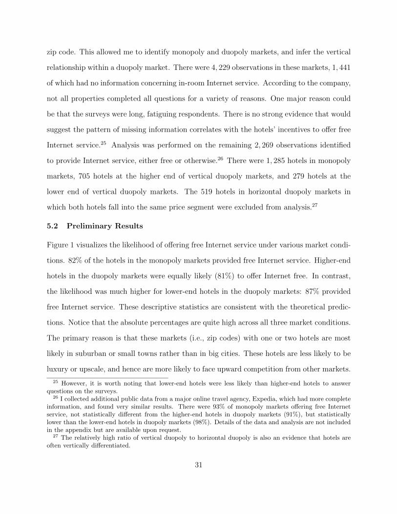
5.2 Preliminary Results

Figure 1 visualizes the likelihood of offering free Internet service under various market condi-

tions. 82% of the hotels in the monopoly markets provided free Internet service. Higher-end

hotels in the duopoly markets were equally likely (81%) to offer Internet free. In contrast,

the likelihood was much higher for lower-end hotels in the duopoly markets: 87% provided

free Internet service. These descriptive statistics are consistent with the theoretical predic-

tions. Notice that the absolute percentages are quite high across all three market conditions.

The primary reason is that these markets (i.e., zip codes) with one or two hotels are most

likely in suburban or small towns rather than in big cities. These hotels are less likely to be

luxury or upscale, and hence are more likely to face upward competition from other markets.

25 However, it is worth noting that lower-end hotels were less likely than higher-end hotels to answerquestions on the surveys.

26 I collected additional public data from a major online travel agency, Expedia, which had more completeinformation, and found very similar results. There were 93% of monopoly markets offering free Internetservice, not statistically different from the higher-end hotels in duopoly markets (91%), but statisticallylower than the lower-end hotels in duopoly markets (98%). Details of the data and analysis are not includedin the appendix but are available upon request.

27 The relatively high ratio of vertical duopoly to horizontal duopoly is also an evidence that hotels areoften vertically differentiated.

31

Furthermore, it is likely that many higher-end hotels offer basic Internet access for free but

charge for heavy uses. These hotels might report free Internet policy even though they were

practicing price discrimination. Therefore, the observed difference in Internet policy between

lower-end and higher-end hotels might be smaller than the actual difference, suggesting that

the analysis is conservative.

A number of factors might have influenced Internet policies. For example, many hotels

have VIP or club floors that target consumers with higher willingness-to-pay. The VIP

floors typically charge customers for higher room rates, but provide additional benefits that

likely include Internet access. These hotels are likely not to offer free Internet service to

all consumers. Another example is that hotels vary in terms of number of rooms. A larger

size likely increases setup, maintenance, or labor costs of supplying Internet service, or the

cost of implementing price discrimination. Other potential confounding factors include the

age, location (i.e., airport, interstate, resort, small town, suburban, or urban), and type of

operation (i.e., chain operated, franchise, or independent) of a hotel.28

I performed regression analysis and control for these possible confounds. The dependent

variable was a binary indicator of whether a hotel offered free Internet service. Indepen-

dent variables were dummies for three market conditions: monopoly, high-end in a vertical

duopoly, and low-end in a vertical duopoly. Monopoly markets were treated as a benchmark

group. The first column of Table 1 suggests that (a) the likelihood of offering free Internet

service at a high-end hotel in a duopoly market was not significantly different from that at

a monopoly hotel, and (b) the likelihood was significantly higher at a lower-end hotel in a

duopoly market in comparison to a monopoly hotel. The second column of the table reports

regression results after controlling for potential confounding factors. Conclusions remained

robust even when these confounds were controlled. Effects of the confounds varied. As ex-

28 There were some hotels with missing information on VIP floor or age. These hotels were flagged in theregressions.

32

pected, hotels with a VIP floor were less likely to offer free Internet service. Larger hotels

were also less likely to offer free Internet service. However, no trend was apparent over the

eight years.

5.3 Higher- versus Lower-end Hotels within a Duopoly

One limitation of the preceding analysis is that market-specific factors are not controlled.

This leads to a noisy comparison among hotels (e.g., a three-star hotel in Boston is compared

to a four-star hotel in New York). It would be useful to examine whether the two hotels in a

vertical duopoly behave differently, a more direct test of the stylized fact. To make within-

market comparison, I restricted attention to duopoly markets in which both hotels reported

their Internet policies.29 There were 86 such duopoly markets. As shown in Figure 3, 74%

of the relatively higher-end hotels provided free Internet service, whereas 88% of the lower-

end competing hotels provided it for free. A paired t-test suggests that this difference was

statistically significant (p = 0.022, t = 2.325). This result suggests that in a market with

vertical differentiation, the lower-quality firm is significantly more likely than its higher-

quality competitor to sell an add-on as standard when it has a very small unit cost.

5.4 Restricting Analysis to Upscale Hotels

Another limitation of the preceding analysis is that the patterns found might be attributed

to the differences in price segments. Next I focused on the segment of upscale hotels. A

hotel in this restricted sample could be in the higher-end condition if there is a mid-priced

or below hotel in the same zip code, or in the lower-end condition if there is a luxury hotel

nearby. A hotel could also be the monopolist in a zip code. There were 646 observations, of

which 355 were monopolists, 250 higher-end, and 41 lower-end.

Figure 2 summarizes the descriptive statistics. The third and fourth columns of Table

1 report the coefficients of the logistic regressions. The results are qualitatively similar to

29 In the preceding analysis, the objective was to compare duopoly markets to monopoly markets. It didnot require both hotels in the same market reported their Internet policies.

33

the preceding analysis. Notice that the higher-end hotels appeared to be more likely to

offer free Internet service than monopoly hotels did. This is most likely because hotels in the

duopoly condition tend to be in urban or suburban areas, which potentially have more luxury

hotels forcing them to free Internet service. The significance of the difference, however, was

weakened when control variables such as location types were included.

Restricting the analysis to the same segment of upscale hotels allows us to rule out several

alternative explanations. One is that higher-end hotels face more heterogeneous consumers

than lower-end hotels do. Presumably the upscale hotels have very similar levels of consumer

heterogeneity across different market conditions. The variation in heterogeneity is unlikely

to explain the patterns observed here. It is also plausible that higher-end hotels tend to

attract consumers who do not anticipate Internet charges, and thus charge a high Internet

price to exploit myopic consumers. Again, the restriction to upscale hotels implies that

the patterns are not attributed to the difference in consumer biases. Another alternative

argument would be that implementing price discrimination costs more at lower-end markets

than at higher-end markets due to efficiency of management, so lower-end hotels tend to

offer free Internet service (no price discrimination). However, the costs presumably do not

differ substantially across the upscale hotels in the sample, and hence the cost explanation

does not seem to support the observed patterns.30

6 Concluding Remarks

Motivated by the seemingly counter-intuitive phenomenon that higher-end hotels are more

likely than lower-end ones to charge for Internet service, I examine the role of vertical differ-

entiation in add-on policies, an element that has been left unexplored in the literature. The

theory uncovers the differential roles of add-ons for vertically differentiated firms. Because

the firms primarily competing for marginal consumers who trade off a higher-quality base

30 The cost explanation is, to some extent, controlled by the variable hotel size (number of rooms in ahotel) in the regressions.

34

good alone versus a lower-quality base good including an add-on, the firm with the higher

base quality focuses on screening consumers, whereas the lower-quality firm has to trade

off screening and differentiation. Surprisingly, selling an add-on as optional can intensify

competition, because the firms price aggressively to attract these marginal consumers.

These insights are particularly relevant to product policy decisions that managers face

in many industries. When a firm sells an add-on in addition to a primary base product,

managers must decide whether they should sell the add-on separately from the base as

optional, or sell it as standard (i.e., free), or not sell it at all. Firms often face competition

in the real-world, both horizontal and vertical. Ignoring any of the two aspects can lead to

misleading policy recommendations. This paper sheds some light on what product policies a

firm should adopt in the presence of vertical differentiation. Managers should evaluate their

add-on policies based on the positioning of their base good. They should consider whether

the base good is differentiated vertically from competitors before designing their add-on

product policy. They should be cautious regarding whether an optional-add-on policy hurts

profit under competition in the long run.

A number of questions remain unaddressed, and may be worth future investigation. First,

the comparative statics implied by Proposition 2 with respect to the cost-to-value ratio of an

add-on provide a direction for future empirical work. Detailed data with exogenous changes

in the cost or value of an add-on are needed for such a study. Second, the proposition

that selling an add-on as optional can hurt profits of vertically differentiated firms is an

interesting hypothesis to test. Unfortunately, the data used in this paper were unsuitable

to test it. Future empirical research into this topic is worth exploring. Third, the theory

focuses on pure vertical differentiation, assuming away horizontal differentiation. In reality,

firms are often differentiated both vertically and horizontally. Further research allowing for

both aspects is interesting.

35

References

Anderson, S. P. and L. Leruth (1993). Why firms may prefer not to price discriminate viamixed bundling. International Journal of Industrial Organization 11 (1), 49–61.

Armstrong, M. and J. Vickers (2001). Competitive price discrimination. The RAND Journalof Economics 32 (4), pp. 579–605.

Armstrong, M. and J. Vickers (2010). Competitive non-linear pricing and bundling. Reviewof Economic Studies 77 (1), 30 – 60.

Bertini, M., E. Ofek, and D. Ariely (2009). The impact of addon features on consumerproduct evaluations. Journal of Consumer Research 36 (1), pp. 17–28.

Champsaur, P. and J.-C. Rochet (1989). Multiproduct duopolists. Econometrica 57 (3), pp.533–557.

Cheema, A. (2008). Surcharges and seller reputation. Journal of Consumer Research 35 (1),pp. 167–177.

Chen, Y., C. Narasimhan, and Z. J. Zhang (2001). Individual marketing with imperfecttargetability. Marketing Science 20 (1), pp. 23–41.

Corts, K. S. (1998). Third-degree price discrimination in oligopoly: All-out competition andstrategic commitment. The RAND Journal of Economics 29 (2), pp. 306–323.

Cruickshank, D. (2000). Review of banking services in the UK. London: HM Treasury .

Dahremoller, C. (2013). Unshrouding for competitive advantage. Journal of Economics &Management Strategy 22 (3), 551–568.

Diamond, P. (1971). A model of price adjustment. Journal of Economic Theory 3 (2),156–168.

Dogan, K., E. Haruvy, and R. Rao (2010). Who should practice price discrimination usingrebates in an asymmetric duopoly?. Quantitative Marketing Economics 8 (1), 61 – 90.

Ellison, G. (2005). A model of add-on pricing. The Quarterly Journal of Economics 120 (2),pp. 585–637.

Gabaix, X. and D. Laibson (2006). Shrouded attributes, consumer myopia, and informationsuppression in competitive markets. The Quarterly Journal of Economics 121 (2), pp.505–540.

Lal, R. and C. Matutes (1994). Retail pricing and advertising strategies. Journal of Business ,345–370.

Matutes, C. and P. Regibeau (1992). Compatibility and bundling of complementary goodsin a duopoly. The Journal of Industrial Economics 40 (1), pp. 37–54.

36

Morwitz, V. G., E. A. Greenleaf, and E. J. Johnson (1998). Divide and prosper: Consumers’reactions to partitioned prices. Journal of Marketing Research 35 (4), pp. 453–463.

Muir, D. M., K. Seim, and M. A. Vitorino (2014). Drip pricing when consumers have limitedforesight: Evidence from driving school fees. Working Paper .

Mussa, M. and S. Rosen (1978). Monopoly and product quality. Journal of EconomicTheory 18 (2), 301–317.

Rochet, J.-C. and L. A. Stole (2002). Nonlinear pricing with random participation. TheReview of Economic Studies 69 (1), pp. 277–311.

Schmidt-Mohr, U. and J. Villas-Boas (2008). Competitive product lines with quality con-straints. Quantitative Marketing Economics 6 (1), 1 – 16.

Shaffer, G. and Z. J. Zhang (1995). Competitive coupon targeting. Marketing Science 14 (4),pp. 395–416.

Shaffer, G. and Z. J. Zhang (2002). Competitive one-to-one promotions. ManagementScience 48 (9), pp. 1143–1160.

Shaked, A. and J. Sutton (1983). Natural oligopolies. Econometrica 51 (5), pp. 1469–1483.

Shugan, S. and N. Kumar (2014). Bundling in product and service lines. Working Paper .

Shulman, J. D. and X. Geng (2012). Add-on pricing by asymmetric firms. ManagementScience.

Stole, L. A. (1995). Nonlinear pricing and oligopoly. Journal of Economics & ManagementStrategy 4 (4), 529–562.

Thisse, J.-F. and X. Vives (1988). On the strategic choice of spatial price policy. TheAmerican Economic Review 78 (1), pp. 122–137.

Tirole, J. (1988). The Theory of Industrial Organization, Volume 1 of MIT Press Books.The MIT Press.

Verboven, F. (1999). Product line rivalry and market segmentation–with an applicationto automobile optional engine pricing. The Journal of Industrial Economics 47 (4), pp.399–425.

37

Figure 1: Vertical Duopoly vs. Monopoly in Small Markets

Figure 2: Vertical Duopoly vs. Monopoly in Small Markets (Upscale Hotels)

Figure 3: Higher- vs. Lower-end Within a Vertical Duopoly

38

Table 1: Regression Results

All Hotels Upscale Hotels Only

No Controls With Controls No Controls With Controls

High-end in Duopoly -0.020 0.101 0.437∗∗ 0.233

(0.121) (0.149) (0.216) (0.276)

Low-end in Duopoly 0.381∗∗ 0.416∗ 1.288∗∗ 1.350∗

(0.191) (0.226) (0.614) (0.781)

VIP Floor -1.486∗∗∗ -1.668∗∗∗

(0.166) (0.320)

No Info on VIP Floor -1.813∗∗∗ -2.315∗∗∗

(0.206) (0.428)

Year 2008 -0.023 -0.388

(0.214) (0.413)

Year 2010 0.271 0.202

(0.224) (0.434)

Year 2012 -0.120 -0.306

(0.233) (0.460)

Location - Interstate -0.042 1.256

(0.422) (0.781)

Location - Resort -0.076 1.673∗

(0.456) (0.980)

Location - Small Town -0.116 1.198∗

(0.364) (0.706)

Location - Suburban -0.414 0.944

(0.321) (0.675)

Location - Urban -0.180 1.813∗∗

(0.355) (0.755)

Operation - Franchised 0.948∗∗∗ 0.229

(0.205) (0.499)

Operation - Independent 0.676∗∗∗ 0.106

(0.258) (0.559)

Size - 75 to 149 rooms -0.309 0.660∗

(0.210) (0.392)

Size - 150 to 299 rooms -1.777∗∗∗ -1.556∗∗∗

(0.228) (0.448)

Size - 300 to 500 rooms -2.726∗∗∗ -2.744∗∗∗

(0.297) (0.622)

Size - >500 rooms -3.447∗∗∗ -3.753∗∗

(0.603) (1.605)

Age -0.003 -0.003

(0.004) (0.006)

No Info on Age 0.482

(2.280)

Observations 2269 2269 646 646

Notes: This table reports the coefficients of the logit model. The dependent variable is whethera hotel offers free Internet service (1 - yes, 0 - no). The benchmark group is the monopolymarkets. Robust standard errors are reported. Significantly different from zero: ∗ for p < .1,∗∗ for p < .05, and ∗∗∗ for p < .01.

39

Online Appendix

to

Add-on Policies under Vertical Differentiation

List of Contents

A. Proof of Lemma 1

B. Proof of Proposition 1

C. Proof of Proposition 2

D. Proof of Proposition 3

E. Proof of Proposition 4

F. Proof of Proposition 5

40

A Proof of Lemma 1

When the Lower-quality Firm Does not Sell the Add-on

Suppose the higher-quality firm sells standard add-on at price P+h . Then the marginal

consumer indifferent between the two firms is: θhl = (P+h −Pl)/(∆V +w). The higher-quality

firm’s profit is Πh = (θ − θhl)(P+h − c). This strategy is exactly equivalent to separating the

bundle price P+h into a base price Ph and an add-on price ph such that P+

h = Ph + ph, and

thatphw

=P+h − Pl

∆V + w=Ph − Pl

∆V. (A-1)

Consider a small increase of the add-on price to p′h = ph + ε with ε > 0, and a small decrease

of the base price to P ′h = Ph−ε by the same amount. The bundle price P+h is then unchanged.

The profit function now becomes

Πh(P′h, p′h) = (θ − P ′h − Pl

∆V)P ′h + (θ − p′h

w)(p′h − c).

Evaluating this function around the original prices (Ph, ph) by Taylor series yields:

Πh(P′h, p′h) = Πh(Ph, ph)− ε · ΠPh

(Ph, ph) + ε · Πph(Ph, ph)

+1

2

[ε2 · ΠPhPh

(Ph, ph) + 2ε2 · ΠPhph(Ph, ph) + ε2 · Πphph(Ph, ph)]

+R2

= Πh(Ph, ph) +ε

∆V(Pl + α∆V )− ε2

w∆V(∆V + w)︸ ︷︷ ︸

M

,

where the second equality follows from the fact that the remainder term R2 is zero because

the higher order derivatives are all zero, and Equation (A-1). Therefore, M > 0 for small ε

when Pl + α∆V > 0.

When the Lower-quality Firm Sells the Add-on

Suppose the higher-quality firm sells standard add-on at price P+h . Then the marginal

consumer indifferent between the two firms is θhl = (P+h − P+

l )/∆V . The higher-quality

firm’s profit becomes Πh = (θ−θhl)(P+h −c). This strategy is exactly equivalent to separating

the bundle price P+h into a base price Ph and an add-on price ph such that P+

h = Ph + ph,

and thatphw

=P+h − P

+l

∆V=Ph − P+

l

∆V − w. (A-2)

41

Consider a small increase of the add-on price to p′h = ph + ε, and a small decrease of the

base price to P ′h = Ph − ε by the same amount. The bundle price P+h is then unchanged.

The profit function now becomes

Πh(P′h, p′h) = (θ − P ′h − P+

l

∆V − w)P ′h + (θ − p′h

w)(p′h − c).

Evaluating this function around the original prices (Ph, ph) by Taylor series yields:

Πh(P′h, p′h) = Πh(Ph, ph)− ε[θ −

Ph − P+l

∆V − w− Ph

∆V − w] + ε[θ − ph

w− ph − c

w] +

ε2

2[− 2

∆V − w− 2

w]

= Πh(Ph, ph) +ε

∆V − w(P+

l + α(∆V − w))− ε2∆V

w(∆V − w)︸ ︷︷ ︸M

where the last equality follows from Equation (A-2). Therefore, M > 0 for small positive ε

when P+l + α(∆V − w) > 0.

B Proof of Proposition 1

Suppose the statement is not true, then in equilibrium the higher-quality firm either (1) sells

standard add-on, or (2) does not sell the add-on at all. In each case there are two possible

equilibria, depending on whether the low quality firm sells the add-on. Next I show that in

each case the higher-quality firm finds it profitable to deviate to selling optional add-on.

When the Higher-quality Firm Sells Standard Add-on

Case (a): the lower-quality firm sells the add-on. The marginal consumer indifferent between

the two firms is θhl = (P+h − P

+l )/∆V . Equilibrium prices are

P+∗h =

1

3∆V (2θ − θ) + c, p∗h < wθ∗hl; P+∗

l =1

3∆V (θ − 2θ) + c, p∗l < wθ∗hl,

with threshold θ∗hl = (θ + θ)/3 > θ. Notice that whether or not the lower-quality firm sells

only the base or the bundle to its lowest-type consumers (i.e., whether p∗l > θ) does not affect

the argument below. Because P+∗l > 0, by Lemma 1 the higher-quality firm can profitably

deviate to selling optional add-on by increasing the add-on price while lowering the base

price.

Case (b): the lower-quality firm does not sell the add-on. The marginal consumer indif-

42

ferent between the two firms is θhl = (P+h − Pl)/(∆V + w). Equilibrium prices are

P+∗h =

1

3(∆V +w)(2θ− θ) +

2

3c, p∗h < wθ∗hl; P ∗l =

1

3(∆V +w)(θ− 2θ) +

1

3c, p∗l > wθ∗hl,

with threshold θ∗ = (θ+θ)/3+c/(3∆V +3w) > θ. Because P ∗l > 0, by Lemma 1 the higher-

quality firm can profitably deviate to selling optional add-on by increasing the add-on price

while lowering the base price.

When the Higher-quality Firm Does not Sell the Add-on

The higher-quality firm’s profit becomes Πh = (θ − θhl)Ph. The threshold θhl is either

(Ph−P+l )/(∆V −w) or (Ph−Pl)/∆V , depending on whether the lower-quality firm sells the

add-on to its highest-type consumers. The best-response prices lead to a threshold θ∗hl < θ.

The higher-quality firm would need to set a high add-on price p∗h > θw so that no one buys

the add-on. However, it is always profitable for the higher-quality firm to lower its add-

on price ph < θw without affecting the profit from selling the base as long as ph > wθ∗hl.

Therefore, no equilibrium exists where the higher-quality firm sells only the base.

C Proof of Proposition 2

I first establish a lemma for the lower-quality firm and then proceed to prove the two cases

of the proposition.

C.1 A Lemma for the Lower-quality Firm

Lemma 2. For the lower-quality firm, not selling the add-on while leaving some consumers

to buy from the higher-quality firm is strictly dominated by selling the add-on, if:

1. Ph > α∆V when the higher-quality firm sells optional add-on, or

2. P+h > α(∆V + w) when the higher-quality firm sells standard add-on.

The proof of the lemma entails a similar argument as in the proof of Lemma 1: (1)

assume the low-quality firm sells only the base, (2) find the equivalent bundle price and

add-on price, (3) consider a small deviation by lowering the bundle price and add-on price,

(4) show that the deviation is profitable. The detail of the proof is available upon request.

C.2 Equilibrium When α ≥ 13(2θ − θ)

In this case the equilibrium profile consists of the following pricing strategies:

P ∗h =1

3(2θ − θ)∆V, p∗h = wθ∗h; P ∗l =

1

3(θ − 2θ)∆V, p∗l > wθ∗hl,

43

where the thresholds are given by θ∗hl = 13(θ + θ) and θ∗h = 1

2(θ + α). Next I establish that

there is no profitable deviation for either firm.

No Profitable Deviation for the Lower-quality Firm

This is established by considering three possible non-local deviations.

Case (a): the lower-quality firm does not sell the add-on and leaves no consumers buy H.

The marginal consumer indifferent between the two firms is θhl = (P+∗h −Pl)/(∆V +w). For

this situation to arise, we need that θhl ≥ p∗h/w so that no consumer buys H. By contrast

the marginal consumer in the equilibrium profile satisfies:

θ∗hl < θ∗h ⇔P ∗h − P ∗l

∆V<p∗hw

=⇒ P+∗h − P ∗l

∆V + w<p∗hw. (C-1)

The lower-quality firm’s profit is given by Πl = (θhl − θ)Pl. It turns out that the optimal

profit under this case is achieved by the corner solution θhl = p∗h/w. To see this, note that

the first order condition of the Lagrangian is given by Pl = (P+∗h − (∆V + w)θ − λ)/2. The

constraint becomes:

θhl −p∗hw

=P+∗h − Pl

∆V + w− p∗hw<P ∗l − Pl∆V + w

=1

2(∆V + w)(−p∗h + wθ + λ),

where the inequality follows from Equation (C-1) and the last equality is obtained by sub-

stituting the best responses of the lower-quality firm. Because p∗h > wθ, to guarantee the

constraint is nonnegative, we need λ > 0. This implies that the constraint has to be binding

by complementary slackness. This corner solution coincides with the corner solution for the

problem under equilibrium because:

P+∗h − Pl

∆V + w=p∗hw

=⇒ P ∗h − Pl∆V

=p∗hw.

Therefore the deviation does not improve the profit.

Case (b): the lower-quality firm sells the add-on and leaves some consumers buy H. The

market is divided into four consumer segments: the consumers θ ∈ [θh, θ] buy H+, the

consumers θ ∈ [θhl, θh] buy H, the consumers with θ ∈ [θl, θhl] buy L+, and the consumers

with θ ∈ [θ, θl] buy L. The thresholds are given by θh = p∗h/w, θhl = (P ∗h−Pl−pl)/(∆V −w),

and θl = pl/w. It will later become evident that when the lower-quality firm sells the add-on

to all of its consumers (i.e., θl < θ) the profit is not improved. Given the higher-quality

firm’s equilibrium pricing the lower-quality firm maximizes profit Πl = (θhl − θ)(P+l − c) −

44

(θl − θ)(pl − c) subject to the constraints: (1) θhl ≥ θl, (2) θl ≥ θ, and (3) θh ≥ θhl.

The objective function is concave and thus the necessary and sufficient condition for

the optimization program is Karush-Kuhn-Tucker conditions. Let λ1, λ2, and λ3 be the

Lagrangian multipliers. The first-order conditions lead to P+l = (P ∗h − (∆V −w)θ+ c−λ1 +

λ3)/2 and pl = (wθ + c− λ1 + λ2)/2. Therefore, Constraint (1) is given by

θhl − θl =1

2w(∆V − w)

[w∆V (

1

3(2θ − θ)− α)− λ2(∆V − w)− λ3w︸ ︷︷ ︸

M

+λ1∆V

].

Because α > (2θ − θ)/3 and both λ2 and λ3 are nonnegative, the term M in the bracket is

strictly negative (M < 0). To guarantee the constraint is nonnegative, we need λ1 > 0. This

implies that Constraint (1) has to be binding. Therefore the profit is no greater than that

obtained from not selling the add-on (i.e., the equilibrium strategy).

It remains to verify that the lower-quality firm would not deviate to selling the add-on

to all of its consumers. In this case its profit is Πl = (θhl − θ)(P+l − c). This profit can

be strictly improved if the firm sets the add-on price pl to be anywhere between [θw, c] so

that some consumers decide not to buy the add-on. The incremental benefit is equal to

−(θl − θ)(pl − c) which is strictly positive.

Case (c): the lower-quality firm sells the add-on but leaves no consumers buy H. The

marginal consumer indifferent between the two firm is θhl = (P+∗h − P+

l )/∆V . To ensure

that no consumers buy H, it is necessary that θhl ≥ p∗h/w. Consider that the lower-quality

firm maximizes profit Πl = (θhl − θ)(P+l − c)− (θl − θ)(pl − c). The profit differs from Case

(b) only in terms of the profit of selling the bundle, (θhl − θ)(P+l − c). Maximizing this

bundling profit under the constraint yields P+l = (P+∗

h −∆V θ + c− λ)/2. Substituting this

best response back to the constraint gives

θhl −p∗hw

=P+∗h − P

+l

∆V− p∗hw

=1

2∆V

[−1

3(θ − 2θ + 3α)∆V +

1

2(θ − α)w︸ ︷︷ ︸

M

+λ].

Because M < 0 when α > (2θ − θ)/3, for the constraint to be nonnegative, it is necessary

that λ > 0. This implies that the constraint has to be binding by complementary slackness.

Therefore the profit is no greater than that obtained from Case (b), which is not a profitable

deviation.

45

No Profitable Deviation for the Higher-quality Firm

Case (a): the higher-quality firm sells optional add-on and leaves some consumers buy L+.

The marginal consumer indifferent between the two firm becomes θhl = (Ph−P ∗l −p∗l )/(∆V −w). Consider the higher-quality firm’s maximization problem Πh = (θ − θh1)Ph + (θ −θh)(ph − c) subject to the constraint θhl ≥ p∗l /w. Notice that the profit function is the

same as the equilibrium one except the threshold θhl. It then suffices to compare the profit

from selling the base only. The first-order condition of the constrained problem is given by

Ph = (P ∗l + p∗l + (∆V − w)θ + λ)/2. Therefore,

θhl −p∗lw

=1

2(∆V − w)[2

3(θ + θ)∆V − θw − p∗l

w(2∆V − w) + λ]

≤ 1

2(∆V − w)[2

3(θ + θ)∆V − θw − 1

3(θ + θ)(2∆V − w) + λ]

=1

2(∆V − w)(−1

3(2θ − θ)w + λ),

where the inequality holds when p∗l > (θ + θ)w/3. Because (2θ − θ) is positive, to ensure

the constraint is nonnegative it is necessary that λ > 0. By complementary slackness the

constraint must be binding, implying that the higher-quality firm leaves no demand for L+.

Therefore, the optimal profit obtained in this case is no greater than the equilibrium profit.

Case (b): the higher-quality firm sells standard add-on and leaves some consumers buy

L+. Because P+∗l > 0, by Lemma 1 this strategy is strictly dominated by a local deviation

whereby the higher-quality firm sells optional add-on by increasing the add-on price while

lowering the base price. This deviation is exactly in the form of Case (a), which yields no

greater profit than the equilibrium one.

Case (c): the higher-quality firm sells standard add-on but leaves no consumers buy L+.

Because P ∗l > 0, by Lemma 1 this strategy is strictly dominated by a local deviation whereby

the higher-quality firm sells optional add-on by increasing the add-on price while lowering

the base price. This local deviation is exactly in the form of the maximization problem in

the equilibrium. Therefore, there is no profitable deviation.

Case (d): the higher-quality firm does not sell the add-on at all. This deviation can take

two forms. First, the higher-quality firm can leave no consumer buy the add-on from the

lower-quality firm. The optimal base price is then the same as the equilibrium strategy P ∗h .

However, since the deviation forgoes the profit from selling the add-on, the deviation profit is

smaller. Second, the higher-quality firm can leave some consumers buy the add-on from the

46

lower-quality firm. The profit is smaller than that in case (a) because a small positive sales

of the add-on can improve profit without affecting profit from the base good. Therefore, in

either case, the deviation is not profitable.

C.3 Equilibrium When α < 13(2θ − θ)

Recall that the equilibrium profile consists of the following pricing strategies:

P ∗h =1

3(2θ − θ)(∆V − w) +

1

3c, p∗h = wθ∗h; P+∗

l =1

3(θ − 2θ)(∆V − w) +

2

3c,

and p∗l = wθ∗l if α > θ but p∗l ≤ wθ∗l if α ≤ θ. The thresholds are given by θ∗hl = (θ + θ)/3−c/(3∆V − 3w), θ∗h = (θ + α)/2, and θ∗l = (θ + α)/2. The next two subsections establish

the second and third statements of the proposition by showing that neither firm will deviate

when ∆V > max{∆1,∆2}. The last subsection shows that no pure strategy equilibrium

exists when ∆V ≤ max{∆1,∆2}.

No Profitable Deviation for the Lower-quality Firm

Case (a): the lower-quality firm does not sell the add-on while leaving some consumers to

buy H. By Lemma 2 this is not a profitable deviation as long as P ∗h > α∆V . Notice that

P ∗h − α∆V =1

3

[(2θ − θ − 3α)∆V − (2θ − θ − α)w

],

which is positive exactly when α < 13(2θ− θ) and ∆V > ∆1. The deviation is not profitable.

Case (b): the lower-quality firm does not sell the add-on and leaves no consumers to buy

H. By Lemma 2 this is not a profitable deviation as long as P+∗h > α(∆V +w). Notice that

P+∗h −α(∆V +w) =

1

3

[(2θ−θ−3α)∆V−(

1

2θ−θ+1

2α)w

]>

1

3

[(2θ−θ−3α)∆V−(2θ−θ−α)w

],

where the inequality follows from α < θ. The last equation is again positive when α <13(2θ − θ) and ∆V > ∆1.

Case (c): the lower-quality firm sells the add-on but leaves no consumers to buy H. The

marginal consumer indifferent between the two firms now becomes θhl = (P+∗h − P

+l )/∆V .

To ensure that no one buys H, the lower-quality firm has to set the bundle price P+l low

enough so that θhl ≥ p∗h/w. By contrast the marginal consumer in the equilibrium profile

satisfies:

θ∗hl < θ∗h ⇔P ∗h − P+∗

l

∆V − w<p∗hw

=⇒ P+∗h − P

+∗l

∆V<p∗hw. (C-2)

47

The lower-quality firm’s profit is given by Πl = (θhl−θ)(P+l −c)−(θl−θ)(pl−c). This profit is

different from the equilibrium one only in terms of the bundling component (θhl−θ)(P+l −c).

The first order condition of the Lagrangian for the constrained maximization of the bundling

profit is given by P+l = (P+∗

h −∆V θ + c− λ)/2. The constraint becomes

θhl −p∗hw

=P+∗h − P

+l

∆V− p∗hw<P+∗l − P

+l

∆V=

1

2∆V(−p∗h + wθ + λ),

where the inequality follows from Equation (C-2) and the last equality is obtained by sub-

stituting the best responses of the lower-quality firm. Because p∗h > wθ, to guarantee the

constraint is nonnegative, we need λ > 0. This implies that the constraint has to be binding.

This corner solution coincides with the one for the problem under the equilibrium because

P+∗h − P

+l

∆V=p∗hw

=⇒ P ∗h − P+l

∆V − w=p∗hw.

Hence, the deviation profit is no greater than that obtained from the equilibrium strategy.

No Profitable Deviation for the Higher-quality Firm

Case (a): the higher-quality firm sells optional add-on but leaves no demand for L+. The the

marginal consumer indifferent between the two firms is θhl = (Ph − P ∗l )/∆V . The higher-

quality firm maximizes profit Πh = (θ − θhl)Ph + (θ − θh)(ph − c) subject to the constraint,

θhl ≤ p∗l /w, so that there is no demand for consumers who buy L+. Note that the profit is

also separable into a component for the base good and a component for the add-on price.

It suffices to examine the profit component of the base good which is different from the

equilibrium one. The first-order condition for the constrained optimization problem of the

base profit is Ph = (P ∗l + ∆V θ − λ)/2. There are two cases to consider. First, if α > θ,

then the equilibrium add-on price is p∗l = (θw + c)/2 and satisfies θ∗hl > θ∗l . The constraint

becomesp∗lw− θhl =

p∗lw− Ph − P ∗l

∆V<P ∗h − Ph

∆V=

1

2∆V(p∗l − θw + λ),

where the inequality follows from θ∗hl > θ∗l , and the last equality is obtained by substituting

the best responses of the higher-quality firm. Because p∗l < θw, for the constraint to be

nonnegative we need λ > 0, implying that the constraint must be binding. The corner

solution is the same as the one under the equilibrium problem because:

Ph − P ∗l∆V

=plw

=⇒ Ph − P+∗l

∆V − w=plw.

48

Therefore the deviation profit is no greater than the equilibrium profit.

Second, if α ≤ θ, then p∗l ≤ θw. There is no demand for the lower-quality firm at all.

The equilibrium strategy is optimal.

Case (b): the higher-quality firm sells standard add-on and leaves some demand for L+.

Because P+∗l > 0, by Lemma 1 this strategy is strictly dominated by selling optional add-on

by increasing the add-on price and lowering the base price. This is exactly the equilibrium

strategy. Therefore, deviation in this case is not profitable.

Case (c): the higher-quality firm sells standard add-on to and leaves no demand for L+.

Because P ∗l > 0, by Lemma 1 this strategy is strictly dominated by selling optional add-on

by increasing the add-on price and lowering the base price. This is exactly the strategy in

Case (a), the profit of which is no greater than the equilibrium profit.

Case (d): the higher-quality firm does not sell the add-on at all. This deviation can

take two forms. First, the higher-quality firm can leave no one buy the add-on from the

lower-quality firm. The profit is smaller than that in case (a) because a small positive sales

of the add-on can improve profit without affecting profit from the base good. Second, the

higher-quality firm can leave some consumers buy the add-on from the lower-quality firm.

The optimal base price is then the same as the equilibrium strategy P ∗h . However, since the

deviation forgoes the profit from selling the add-on, the deviation profit is smaller than the

equilibrium profit. Therefore, in either case, the deviation is not profitable.

No Pure Strategy Equilibrium Exists When ∆V ≤ max{∆1,∆2}

Because in equilibrium the higher-quality firm will always sell the add-on as optional by

Proposition 1, there are two possible equilibrium outcomes depending on the lower-quality

firm’s implementation: (a) the lower-quality firm sells the add-on, and (b) the firm does not

sell the add-on at all. Neither case is sustainable when ∆V ≤ max{∆1,∆2}.Case (a): the lower-quality firm sells the add-on. The equilibrium profiles are the same

as those in the second and the third statements of the proposition. When α > θ, both firms

sell optional add-on. The fraction of consumers who buy the bundle from the lower-quality

firm is given by

θ∗hl − θ∗l =1

6(∆V − w)

[(2θ − θ − 3α)∆V − (2θ − θ − α)w

],

which is positive only if ∆V > ∆1.31

When α ≤ θ, the lower-quality firm will sell the add-on as standard, and the fraction of

31Note that ∆1 > ∆2 when α > θ, and ∆2 > ∆1 when α < θ.

49

consumers who buy the bundle from the lower-quality firm becomes

θ∗hl − θ =1

3(∆V − w)

[(θ − 2θ)∆V − (θ − 2θ + α)w

].

which is positive only if ∆V > ∆2.

Case (b): the lower-quality firm does not sell the add-on at all. In this case, the equilib-

rium profile is the same as that in the first statement of the proposition. The higher-quality

firm’s base price is then P ∗h = (2θ − θ)∆V/3. Since α < (2θ − θ)/3, we have P ∗h > α∆V .

Therefore, by Lemma 2 the lower-quality firm can profitably deviate by selling the add-on.

D Proof of Proposition 3

D.1 Second-stage Pricing Game

First observe that the higher-quality firm will never commit to no-add-on policy. By commit-

ting to not selling the add-on, the higher-quality firm always uses the base good to compete

with the lower-quality firm in the second stage. Deviating to not making the commitment

allows it to sell the add-on to a fraction of consumers who have the highest taste for qual-

ity. This does not affect the profit from selling the base good but can gain some additional

benefit from selling the add-on. Profit is then strictly improved. Therefore, committing to

no-add-on policy is always strictly dominated by not committing.

Second, when the higher-quality firm does not commit to standard add-on, it retains

the flexibility of selling the add-on as optional. The equilibrium outcomes are the same as

those summarized in Proposition 2. The difference is that here the lower-quality firm can

not deviate to selling optional add-on in the second-stage pricing game once it has made

the commitment to either standard-add-on or no-add-on policies. The equilibrium outcome

depends on each of the three commitment choices of the lower-quality firm.

When the lower-quality firm commits to no-add-on policy, the equilibrium pricing in the

second stage is the same as that in the first case of Proposition 2. The resulting profits are

given by Π(opt,no)h and Π

(opt,no)l .

When the lower-quality firm commits to standard-add-on policy, the equilibrium pricing

is the same as that in the third case of Proposition 2. The resulting profits are given by

Π(opt,std)h and Π

(opt,std)l .

When the lower-quality firm does not commit, the equilibrium pricing is the same as that

in the second case of Proposition 2. The resulting profits are given by Π(opt,opt)h and Π

(opt,opt)l .

Third, when the higher-quality firm commits to standard-add-on policy, it commits to a

50

uniform price P+h that bundles the base good and the add-on. In the second-stage pricing

game, the firm cannot sell the add-on separately to screen consumers. The equilibrium

outcome depends on each of the three commitment choices of the lower-quality firm.

When the lower-quality firm commits to no-add-on policy, the equilibrium pricing in the

second stage now becomes

P+∗h =

1

3(2θ − θ)(∆V + w) +

2

3c, P ∗l =

1

3(θ − 2θ)(∆V + w) +

1

3c,

and the marginal consumer is given by θ∗hl = (θ + θ)/3 + c/(3∆V + 3w). The incentive

constraints θ > θ∗hl > θ hold given that θ > 2θ. The resulting profits are given by Π(std,no)h

and Π(std,no)l .

When the lower-quality firm commits to standard-add-on policy, the second-stage pricing

becomes

P+∗h =

1

3(2θ − θ)∆V + c, P+∗

l =1

3(θ − 2θ)∆V + c,

and the marginal consumer is given by θ∗hl = (θ+θ)/3. The incentive constraints θ > θ∗hl > θ

hold given that θ > 2θ. The resulting profits are given by Π(std,std)h and Π

(std,std)l .

When the lower-quality firm does not commit, the second-stage pricing becomes

P+∗h =

1

3(2θ − θ)∆V + c, P+∗

l =1

3(θ − 2θ)∆V + c, p∗l = wθ∗l

where the marginal consumers are given by θ∗hl = (θ+θ)/3 and θ∗l = (θ+α)/2. The incentive

constraints θ > θ∗hl > θ∗l > θ hold given that θ > 2θ and θ < α < (2θ − θ)/3. The resulting

profits are given by Π(std,opt)h and Π

(std,opt)l .

D.2 First-stage Commitment Choices

The Higher-quality Firm Commits to Standard Add-on

First, when the lower-quality firm commits to not selling the add-on, the higher-quality firm

is better off to commit to standard add-on because the improvement in profit is positive

Π(std,no)h − Π

(opt,no)h =

w

9

[(2θ − θ)2 − 2α(2θ − θ)− 9

4(θ − α)2︸ ︷︷ ︸

=X>0

+α2w

∆V + w

]> 0.

Second, when the lower-quality firm sells the add-on, the higher-quality firm’s profit is

unaffected by whether its rival commits to standard add-on or not. This is because in either

51

case the higher-quality firm is competing with its rival’s bundle good. The firm, however,

benefits from committing to standard add-on as long as the quality premium is large enough.

The improvement in profit becomes

Π(std,opt)h − Π

(opt,opt)h =

w

9

[(2θ − θ)2 − 2α(2θ − θ)− 9

4(θ − α)2︸ ︷︷ ︸

=X>0

− α2w

∆V − w

]. (D-1)

which is increasing in the quality premium ∆V and is positive if ∆V = (1 + α2/X)w ≡ ∆3.

The Lower-quality Firm Commits to No Add-on

Given that the higher-quality firm commits to standard add-on, it remains to consider the

three possibilities depending on the lower-quality firm’s commitment choices. First, note

that committing to standard add-on is dominated by not committing, Π(std,opt)l > Π

(std,std)l .

This is because the lower-quality firm is selling the add-on to its higher-type consumers

anyway, the commitment choice does not matter for the competition with its rival. This is

very different from the higher-quality firm’s problem.

Second, selling optional add-on is dominated by committing to not selling it. To see that,

the benefit from commitment is given by

Π(std,no)l − Π

(std,opt)l =

w

9

[(θ − 2θ)2 + 2α(θ − 2θ)− 9

4(θ − α)2︸ ︷︷ ︸

Y

+α2w

∆V − w

]. (D-2)

which is also increasing in the quality premium ∆V . It can be shown that Y > 0 when

θ < α < 13(2θ − θ). Therefore, Π

(std,no)l > Π

(std,opt)l .

Therefore, there exists an equilibrium of the full game such that the higher-quality firm

commits to standard add-on, while the lower-quality firm commits to no add-on, provided

the quality premium is large enough such that ∆V > max{∆1,∆3}.

E Proof of Proposition 4

E.1 When α < (θ + θ)/3

For the equilibrium in which the low-quality firm sells the add-on as optional to exist, the

following incentive constraints have to be satisfied: (a) θ∗hl > θ∗l ; (b) θ∗l > θ ⇒ θ∗hl > 2θ − α.

For the equilibrium in which the low-quality firm sells the add-on as standard to exist, it

requires that (c) θ∗hl > θ; (d) θ∗l < θ. Note that (a) and (b) imply (c). Define the following

52

quantities:

∆(u)0 =

θ − 2θ + α

θ − 2θ· w, ∆

(u)1 =

2θ + θ − 3α

2(θ + θ − 3α)· w, and ∆

(u)2 =

2θ − 9θ + 7α

2(θ − 5θ + 3α)· w.

Constraint (a) is equivalent to θ∗hl > α since θ∗l = 12(θ∗hl + c). Note that θ∗hl−α is positive

as long as ∆V > ∆(u)1 . Constraint (b) is equivalent to θ∗hl > 2θ − α since θ∗l = 1

2(θ∗hl + α).

Note that θ∗hl − (2θ − α) is positive as long as ∆V > ∆(u)2 . Note further that ∆

(u)1 > ∆

(u)2 is

equivalent to 2(α − θ)(θ − 2θ + 6α) > 0, which holds if and only if α > θ. Therefore, if the

lower-quality firm sells optional add-on in equilibrium, then either one of the following must

hold: (1) α > θ and ∆V > ∆(u)1 , or (2) α < θ and ∆V > ∆

(u)2 .

Finally, if the lower-quality firm sells standard add-on in equilibrium, Constraint (c) gives

θ∗(u)hl − θ =

(θ − 2θ)∆V − (θ − 2θ + α)w

6∆V − 5w> 0⇐⇒ ∆V > ∆

(u)0 .

To satisfy Constraint (d), it suffices that ∆V < ∆(u)2 . Note that ∆

(u)2 > ∆

(u)0 is equivalent to

(θ− α)(θ− 2θ + 6α) > 0, which always holds when α < θ. It remains to verify that there is

no profitable deviation from either firm.

No Profitable Deviation for the Lower-quality Firm

The only non-local deviation is that the lower-quality firm does not leave demand for H.

Fixing the higher-quality firm’s equilibrium prices, (P ∗h , pe∗h ), and given the lower-quality

firm’s total price, P+l , the consumers with θ ∈ [θ, θhl] choose to pay the base price to visit

the lower-quality firm at time t = 1. The marginal consumer is given by θhl = (P+∗h −P

+l )/V

. At time t = 2, these consumers observe the ad-on price pl and decide whether to buy it or

not. The firm maximizes its ex post profit, πl = (θhl − θl)(pel − c) with θl = pel /w. Again,

the optimal strategy by the firm is to set θl as a function of the marginal consumer θhl:

θl(θhl) = (θhl + α)/2.

The firm’s problem at time t = 0 is then finding the optimal θhl that maximizes the total

profit taking into account the second-period problem

maxθhl

(θhl − θ)(P+∗h − θhl∆V︸ ︷︷ ︸

=Pl+pel

−c)− (θl(θhl)− θ)(w · θl(θhl)− c).

53

The (unconstrained) optimal choice of the marginal consumer is

θdhl =2P+∗

h − 2c+ (2∆V + w)θ

4∆V + w.

This deviation requires that no consumer would buy only the base good from the higher-

quality firm, that is, θdhl ≥ θ∗h. However, notice that

θdhl − θ∗h =−4(θ − 2θ + 3α)∆V 2 − (θ − 2θ − 5α)w∆V + 7

2(θ − 2θ + α)w2

(4∆V + w)(6∆V − 5w),

which is negative because ∆V > w. Therefore, the optimal solution is binding such that

θhl = θ∗h. Hence, the lower-quality firm has no incentive to deviate.

No Profitable Deviation for the Higher-quality Firm

The only non-local deviation that could be profitable is that the higher-quality firm imple-

ments the standard add-on policy. Since it is always optimal for the higher-quality firm

to set the add-on price, pe∗h = (θw + c)/2, that maximizes ex post profit, the deviation is

achieved by increasing the base price so that no consumer will buy the base good. In the

first case, the firm deviates by charging the total price P+h = Ph + pe∗h at t = 0 while leaving

some demand for L+. The optimal deviation is P+dh = 1

2(P+∗

l + ∆V θ + c). The profit from

this deviation, Πdh, is no greater than the equilibrium profit because

Π∗h − Πdh =

[w[P+∗l + θ(∆V − w)

]− (∆V − w)(θw − c)

]2

4(∆V − w)w∆V

is non-negative. In the second case, the firm charges P+h such that there is no demand for

L+. The optimal deviation is P+dh = (P ∗l +∆V (θ+w)+c)/2. The profit from this deviation,

Πd′

h is no greater than the deviation profit in the first case, because

Πdh − Πd′

h =1

4∆V

[P+∗l + θ∆V − c︸ ︷︷ ︸

=A+B

]2 − 1

4(∆V + w)

[P ∗l + θ(∆V + w)− c︸ ︷︷ ︸

=A

]2=B2(∆V + w) + 2AB(∆V + w) + A2w

4(∆V + w)∆V

is non-negative given that A+B > 0 and B < 0. Therefore, there is no profitable deviation

for the higher-quality firm.

54

E.2 When α ≥ (θ + θ)/3

In this case, the equilibrium prices are exactly the same as case (1) in Proposition 2 (see

subsection C.2 in the Appendix), except that the add-on price at the higher-quality firm

is unobserved but correctly expected by rational consumers. Therefore, as long as α ≥(2θ − θ)/3, there is no profitable deviation from either firm. However, when α ∈ ((θ +

θ)/3, (2θ− θ)/3), the lower-quality firm can profitably deviate by selling the add-on to some

consumers.

F Proof of Proposition 5

Let superscripts “o” and “u” denote the observed-price and the unobserved-price cases.

F.1 Market Shares

The difference in the marginal consumers indifferent between the two firms is

θ∗(u)hl − θ

∗(o)hl = −

[(θ − 2θ)∆V − (θ − 2θ + α)w

]w

3(∆− w)(6∆V − 5w)< 0.

The inequality follows from ∆V > ∆(u)0 . The difference in the marginal consumers indiffer-

ence between buying the add-on and not buying is

θ∗(u)l − θ∗(o)l =

1

2(θ∗(u)hl − θ) =

(θ − 2θ)∆V − (θ − 2θ + α)w

6∆V − 5w> 0.

The inequality holds if and only if ∆V > ∆(u)0 . Therefore the lower-quality firm is losing

consumers who buy the add-on.

F.2 Prices

The difference in the base prices of the higher-quality firm is given by:

P∗(u)h − P ∗(o)h =

w(∆V − w)(θ − 2θ + 6α)

3(6∆V − 5w)> 0.

Therefore the higher-quality firm charges higher base price when the add-on prices are not

observed. The difference in the add-on prices of the lower-quality firm is given by:

p∗(u)l − p∗(o)l =

1

2(θ∗(u)hl − θ)w =

[(θ − 2θ)∆V − (θ − 2θ + α)w

]w

6∆V − 5w> 0,

55

where the inequality follows from ∆V > ∆(u)0 . Therefore the lower-quality firm charges a

higher add-on price under the unobserved-price equilibrium.

Note that under either unobserved-price or observed-price equilibrium, the indifference

condition and the higher-quality firm’s best response satisfy:P+∗l = P ∗h − θ∗hl(∆V − w)

P ∗h = 12(P+∗

l + θ(∆V − w))⇒ P+∗

l = (∆V − w)(θ − 2θ∗hl). (F-1)

With some algebras, the difference in the total prices is positive: P+∗(u)l − P+∗(o)

l = 2(∆V −w)(θ

∗(o)hl − θ

∗(u)hl ) > 0. The difference in the base price is given by

P∗(u)l −P ∗(o)l = 2(∆V −w)(θ

∗(o)hl − θ

∗(u)hl )− 1

2(θ∗(u)hl −θ)w = −

w[(θ − 2θ)∆V − (θ − 2θ + α)w

]3(6∆V − 5w)

,

which is negative given that ∆V > ∆(u)0 .

F.3 Profits

The higher-quality firm’s profit is clearly increased because it sells the base to more consumers

at a higher price while keeping the add-on profit unchanged. For the lower-quality firm, the

profit difference is given by

∆Πl = (θ∗(u)hl −θ)(P

+∗(u)l −c)−(θ

∗(u)l −θ)(p∗(u)

l −c)−(θ∗(o)hl −θ)(P

+∗(o)l −c)+(θ

∗(o)l −θ)(p∗(o)l −c).

Let

B =

[(θ − 2θ)∆V − (θ − 2θ + α)w

]w

3(∆− w)(6∆V − 5w).

Then from the above results imply θ∗(u)hl = θ

∗(o)hl −B, θ

∗(u)l = θ

∗(o)l + 3B(∆− w)/w, P

+∗(u)l =

P+∗(o)l + 2(∆ − w)B, and p

∗(u)l = p

∗(o)l + 3(∆ − w)B. Substituting these quantities into the

profit difference yields ∆Πl = −(3∆V − 2w)(∆V −w)B2/w < 0, where the equality follows

from 3∆V > 2w.

56