Towards Finding Optimal Differential Characteristics for ARX

IntroductionAutomatic differentiation of prototypical numerical integration algorithms
Experimental results with a one-mass oscillatorApplication to a technical system
Conclusions
Automatic differentiation of numerical integrationalgorithms
after Peter Eberhard, Christian Bischof
Zofia Mączyńska
21. August 2006
Zofia Mączyńska Numerical integration algorithms
IntroductionAutomatic differentiation of prototypical numerical integration algorithms
Experimental results with a one-mass oscillatorApplication to a technical system
Conclusions
Outline
Introduction
Automatic differentiation of prototypical numerical integrationalgorithms
Experimental results with a one-mass oscillator
Application to a technical system
Conclusions
Zofia Mączyńska Numerical integration algorithms

IntroductionAutomatic differentiation of prototypical numerical integration algorithms
Experimental results with a one-mass oscillatorApplication to a technical system
Conclusions
Introduction
Zofia Mączyńska Numerical integration algorithms

IntroductionAutomatic differentiation of prototypical numerical integration algorithms
Experimental results with a one-mass oscillatorApplication to a technical system
Conclusions
We will present the application of automatic differentiation tonumerical integration algorithms for ODE’s, in particular theramifications of the fact that AD is applied not only to thesolution but also to the solution procedure itself.
Zofia Mączyńska Numerical integration algorithms

IntroductionAutomatic differentiation of prototypical numerical integration algorithms
Experimental results with a one-mass oscillatorApplication to a technical system
Conclusions
mathematical model of technical systems or naturalphenomena
Initial value problem, ODEFor given values of system parameters p ∈ Rh, find the trajectoriesx(t, p), x ∈ Rn for t0 ≤ t ≤ t1, where x is the state vector, t thetime. The state is determined by the solution of the initial valueproblem:
x = f (x , p, t), x(t = t0, p) = x0,
where f is the vector of state derivatives, x0 the initial state, t0
and t1 the initial and final time respectively.
Zofia Mączyńska Numerical integration algorithms

IntroductionAutomatic differentiation of prototypical numerical integration algorithms
Experimental results with a one-mass oscillatorApplication to a technical system
Conclusions
The ODE is typically solved by using numerical integrationalgorithms. In engineering applications one is not only interested inthe final state but also in the performance criteria ψ computed fromthe trajectories x. If optimization procedures are applied on order tochoose optimal design variables with respect to certain performancecriteria, or if parameter estimation techniques are used to identifymodel parameters from measurements, then, with the final state
x1 := x(t1, p)
one typically has to compute
∂x1
∂pT .
Zofia Mączyńska Numerical integration algorithms

IntroductionAutomatic differentiation of prototypical numerical integration algorithms
Experimental results with a one-mass oscillatorApplication to a technical system
Conclusions
The numerical value of the sensitivities at the final step maydepend on the whole history of the system.
Zofia Mączyńska Numerical integration algorithms

IntroductionAutomatic differentiation of prototypical numerical integration algorithms
Experimental results with a one-mass oscillatorApplication to a technical system
Conclusions
I AD tools have been developed to make it possible to augmentgeneral Fortran or C codes with statements for thecomputation of derivatives in an automated fashion.
I AD is based on the fact that every computer program employsonly the simplest operations (addition, multiplication, sin,etc.) whose derivatives are known.
I AD computes the derivatives for the whole programm and thencompose them using the chain rule of differential calculus.
Zofia Mączyńska Numerical integration algorithms

IntroductionAutomatic differentiation of prototypical numerical integration algorithms
Experimental results with a one-mass oscillatorApplication to a technical system
Conclusions
Watch out!
AD differentiate not only the solution computed by a programm,but also the algorithm by which the solution is being derived. Thus,the value of the derivative may depend on the algorithm chosen tocompute the solution.
Zofia Mączyńska Numerical integration algorithms

IntroductionAutomatic differentiation of prototypical numerical integration algorithms
Experimental results with a one-mass oscillatorApplication to a technical system
Conclusions
PLAN
We will:1. consider AD of a prototypical integration algorithm and
illustrate how different integrators can lead to different valuesof computed derivatives
2. suggest two approaches to suppress the impact of the solutionalgorithm on derivatives
Zofia Mączyńska Numerical integration algorithms

IntroductionAutomatic differentiation of prototypical numerical integration algorithms
Experimental results with a one-mass oscillatorApplication to a technical system
Conclusions
Automatic differentiation ofprototypical numerical integration
algorithms
Zofia Mączyńska Numerical integration algorithms
IntroductionAutomatic differentiation of prototypical numerical integration algorithms
Experimental results with a one-mass oscillatorApplication to a technical system
Conclusions
Algorithms for numerical integration of ODEs:1. single step2. multistep3. extrapolation4. special (for stiff systems, highly or loosely coupled systems,
systems composed of several subsystems, etc.)
Zofia Mączyńska Numerical integration algorithms

IntroductionAutomatic differentiation of prototypical numerical integration algorithms
Experimental results with a one-mass oscillatorApplication to a technical system
Conclusions
We will illustrate the interplay of the AD and the integrationalgorithms (single-step algorithm of Euler and Runge-Kutta typewith and without stepsize control and a sophisticated multistepintergation algorithm with adaptive stepsize control andinterpolation order control.)
Zofia Mączyńska Numerical integration algorithms

IntroductionAutomatic differentiation of prototypical numerical integration algorithms
Experimental results with a one-mass oscillatorApplication to a technical system
Conclusions
single-step algorithmTime discretization applied to x = f (x , p, t), x(t = t0, p) = x0
leads to a recursive scheme:
xi+1 = xi + hi ˙xi
ti+1 = ti + hi ,
where:i denotes the ith integration step, xi := x(ti ), hi is the actualstepsize, ˙x denotes slope estimation.Two cases are possible:
I hi = h = const leads to the Euler schemeI dynamically adaptive stepsize control (based on local error
estimates).
Zofia Mączyńska Numerical integration algorithms

IntroductionAutomatic differentiation of prototypical numerical integration algorithms
Experimental results with a one-mass oscillatorApplication to a technical system
Conclusions
multistep algorithm
Multistep algorithms additionally use the information from formersteps to predict the appropriate stepsizes and slopes.
Zofia Mączyńska Numerical integration algorithms

IntroductionAutomatic differentiation of prototypical numerical integration algorithms
Experimental results with a one-mass oscillatorApplication to a technical system
Conclusions
All variables inxi+1 = xi + hi ˙xi
may depend on p.This leads to:
xi+1(p) = xi (p) + hi (p) ˙xi (p)
Zofia Mączyńska Numerical integration algorithms

IntroductionAutomatic differentiation of prototypical numerical integration algorithms
Experimental results with a one-mass oscillatorApplication to a technical system
Conclusions
Differentiatingxi+1(p) = xi (p) + hi (p) ˙xi (p)
with respect to p with ∇x := dxdpT gives:
∇xi+1 = ∇xi + hi∇ ˙xi +∇hi ˙xi .
Zofia Mączyńska Numerical integration algorithms

IntroductionAutomatic differentiation of prototypical numerical integration algorithms
Experimental results with a one-mass oscillatorApplication to a technical system
Conclusions
Computation of the desired derivatives for the state variables
To obtain the desired derivatives we can consider two choices:I manual transformationI automatic transformation with AD tools
Zofia Mączyńska Numerical integration algorithms

IntroductionAutomatic differentiation of prototypical numerical integration algorithms
Experimental results with a one-mass oscillatorApplication to a technical system
Conclusions
Zofia Mączyńska Numerical integration algorithms

IntroductionAutomatic differentiation of prototypical numerical integration algorithms
Experimental results with a one-mass oscillatorApplication to a technical system
Conclusions
Differentiatingx = f (x , p, t)
with respect to p we obtain (with dtdpt = 0):
ddpT (x) =
ddpT (
dxdt
) =∂f∂xT
dxdpT +
∂f∂pT
Exchanging the order of differentiation we obtain a new ODE for∇x :
ddt
(dx
dpT ) =ddt
(∇x) = [∇x ] =∂f∂xT ∇x+
∂f∂pT , ∇x(t = t0) = ∇x0,
which we can integrate alongside our original solution. ADtechniques could be employed to compute ∂f
∂xT and ∂f∂pT but we
would not integrate through the integration algorithm for x .
Zofia Mączyńska Numerical integration algorithms

IntroductionAutomatic differentiation of prototypical numerical integration algorithms
Experimental results with a one-mass oscillatorApplication to a technical system
Conclusions
observation
The stepsize hi is likely to depend on the parameters p and the ADtool will associate a gradient ∇hi with hi . Thus, the update∇xi+1 = ∇xi + hi∇ ˙xi +∇hi ˙xi , which will be computed by an ADtool, leads to an inconsistent integrator for ∇x , as the final resultdepends on the discretization strategy chosen. Hence it is alsounlikely that ∇x1 = ∇x |(ti=t1) equals the desired ∂x1
∂pT .
Zofia Mączyńska Numerical integration algorithms

IntroductionAutomatic differentiation of prototypical numerical integration algorithms
Experimental results with a one-mass oscillatorApplication to a technical system
Conclusions
The automatically differentiated integration algorithm computesx1(t1(p), p) (the dependence of t1 on p results only from theadaptive time discretization). Differentiating with respect to p weobtain:
∇x1 =∂x1
∂t1∇t1 +∂x1
∂pT
The green depend on the time discretization and are computed bythe AD generated code. Thus, to arrive at the desired solution ∂x1
∂pT ,we can pursue one of the following strategies:
Zofia Mączyńska Numerical integration algorithms

IntroductionAutomatic differentiation of prototypical numerical integration algorithms
Experimental results with a one-mass oscillatorApplication to a technical system
Conclusions
∇x1 =∂x1
∂t1∇t1 +∂x1
∂pT
We can pursue one of the following strategies:I Perform a posteriori error correction:
The desired derivatives ∂x1
∂pT , which don’t depend on the timediscretization can be computed as:
∂x1
∂pT = ∇x1 − f (x1, p, t1)∇t1.
I Use an integrator with fixed stepsize:In this case, we have: ∇hi ≡ 0,∀i . Thus ∇t ≡ 0 and hence:∇x1 ≡ ∂x1
∂pT . The AD-computed derivative trajectories are thedesired ones, and thus, no modification is required for fixedstepsize integration algorithms.
Zofia Mączyńska Numerical integration algorithms

IntroductionAutomatic differentiation of prototypical numerical integration algorithms
Experimental results with a one-mass oscillatorApplication to a technical system
Conclusions
∇x1 =∂x1
∂t1∇t1 +∂x1
∂pT
We can pursue one of the following strategies:I Perform a posteriori error correction.I Use an integrator with fixed stepsize.I Modify the AD-generated code to enforce ∇hi = 0∀i :
I For the first step the user must guess the initial step h0I h0 independent of p, thus ∇h0 = 0I Assume that the correct stepsize h is known in advance for
each step. Then ∇hi = 0∀i and we get the same correctresults as for the fixed stepsize algorithm.
Zofia Mączyńska Numerical integration algorithms
IntroductionAutomatic differentiation of prototypical numerical integration algorithms
Experimental results with a one-mass oscillatorApplication to a technical system
Conclusions
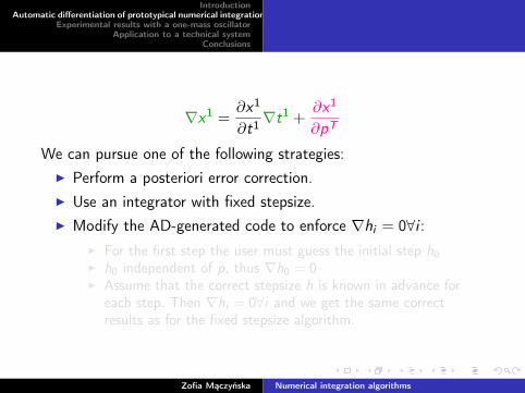
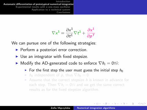
∇x1 =∂x1
∂t1∇t1 +∂x1
∂pT
We can pursue one of the following strategies:I Perform a posteriori error correction.I Use an integrator with fixed stepsize.I Modify the AD-generated code to enforce ∇hi = 0∀i :
I For the first step the user must guess the initial step h0I h0 independent of p, thus ∇h0 = 0I Assume that the correct stepsize h is known in advance for
each step. Then ∇hi = 0∀i and we get the same correctresults as for the fixed stepsize algorithm.
Zofia Mączyńska Numerical integration algorithms

IntroductionAutomatic differentiation of prototypical numerical integration algorithms
Experimental results with a one-mass oscillatorApplication to a technical system
Conclusions
Experimental results with a one-massoscillator
Zofia Mączyńska Numerical integration algorithms

IntroductionAutomatic differentiation of prototypical numerical integration algorithms
Experimental results with a one-mass oscillatorApplication to a technical system
Conclusions
the simplest multibody system
We consider a horizontal one-mass oscillator. One can derivesolutions for both, that state and its gradients, and thus it is a wellsuited example for us.
Zofia Mączyńska Numerical integration algorithms
IntroductionAutomatic differentiation of prototypical numerical integration algorithms
Experimental results with a one-mass oscillatorApplication to a technical system
Conclusions
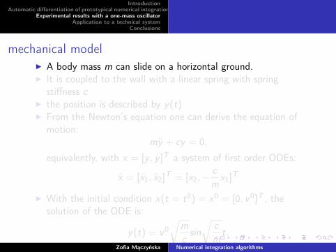
mechanical modelI A body mass m can slide on a horizontal ground.I It is coupled to the wall with a linear spring with spring
stiffness cI the position is described by y(t)I From the Newton’s equation one can derive the equation of
motion:my + cy = 0,
equivalently, with x = [y , y ]T a system of first order ODEs:
x = [x1, x2]T = [x2,−
cm
x1]T
I With the initial condition x(t = t0) = x0 = [0, v0]T , thesolution of the ODE is:
y(t) = v0√
mc
sin√
cm
t.Zofia Mączyńska Numerical integration algorithms

IntroductionAutomatic differentiation of prototypical numerical integration algorithms
Experimental results with a one-mass oscillatorApplication to a technical system
Conclusions
For m = 1 and the system parameters p = [c, v0] we find:
y(t) = v0 1√csin√
ct,
y(t) = v0cos√
ct,
y(t) = −v0√csin√
ct.
Zofia Mączyńska Numerical integration algorithms

IntroductionAutomatic differentiation of prototypical numerical integration algorithms
Experimental results with a one-mass oscillatorApplication to a technical system
Conclusions
We now define two criteria:I The criterion ψ1 contains the position of the body at the time
t1 = π2 .
For p = [1, 0.5]T we have:
dψ1
dp1=
dψ1
dc= . . . = −0.25,
dψ1
dp2=
dψ1
dv0 =1√csin(
√cπ
2) = 1.0.
I The criterion ψ2 integrates the position over the wholeinteresting simulation time interval [t0, t1]:
ψ2 =
∫ t1
t0y(t)dt =
∫ t1=π2
t0=0
v0√
csin√
ct.
Explicit solution for the gradients:
ψ2
dp1=ψ2
dc= . . . =
π
8− 1
2,ψ2
dp2=
ψ2
dv0 = . . . = 1.0.
Zofia Mączyńska Numerical integration algorithms

IntroductionAutomatic differentiation of prototypical numerical integration algorithms
Experimental results with a one-mass oscillatorApplication to a technical system
Conclusions
Single-step integration without stepsize control
I We investigate and compare three similar integration schemes:Euler scheme, the Heun algorithm, and the 4th orderRunge-Kutta algorithm.
I Result:I Only minor differences between the reference gradient and the
AD gradient existsI The relative error in the criteria is about the size of the error
on the gradients
I Explanation: As expected AD of single-step integrationalgorithms without stepsize control leads to the desired resultswithout any need for user modification. The differnties can beexplained by the choice of the stepsize and the algorithm, noadditional errors are introduced in the AD procedure.
Zofia Mączyńska Numerical integration algorithms

IntroductionAutomatic differentiation of prototypical numerical integration algorithms
Experimental results with a one-mass oscillatorApplication to a technical system
Conclusions
Single step integration algorithms with adaptive stepsizecontrol
We consider a mixed 4th and 5th order Runge-Kutta algorithmwith stepsize control.The error ∆ is of magnitude h5, thus we can estimate the requiredstepsize h from the desired error bound ∆, the actual stepsize hand the actual error ∆:
h5
∆≈ h5
∆⇒ h ≈ h
5
√∆
∆
Zofia Mączyńska Numerical integration algorithms

IntroductionAutomatic differentiation of prototypical numerical integration algorithms
Experimental results with a one-mass oscillatorApplication to a technical system
Conclusions
If h > h, the actual stepsize was too big and the step has to berepeated with decreased stepsize until the the error estimate isacceptable. Otherwise the next step is computed and theintegration proceeds.
Zofia Mączyńska Numerical integration algorithms

IntroductionAutomatic differentiation of prototypical numerical integration algorithms
Experimental results with a one-mass oscillatorApplication to a technical system
Conclusions
I The actual stepsize hi and the actual time ti depend n thestate xi and therefore on the system parameters p, so the ADtool will compute the gradients ∇hi = dhi
dpT and ∇ti = dtidpT .
I We then employ the relation ∂x1
∂pT = ∇x1 − f (x1, p, t1)∇t1 to
compute (at every time step) the desired ∂x∂pT from ∇x and
∇t.
Zofia Mączyńska Numerical integration algorithms

IntroductionAutomatic differentiation of prototypical numerical integration algorithms
Experimental results with a one-mass oscillatorApplication to a technical system
Conclusions
multistep integration algorithm (Shampine-Gordon)
In a multistep algorithm the information already available fromprevious steps is used to predict further steps. (The integrationalgorithm consists of about 900 lines of code and therefore themanual modification of the code to ensure ∇hi = 0 is not a reliableapproach, the a posteriori error correction is used instead and itleads to correct results.
Zofia Mączyńska Numerical integration algorithms

IntroductionAutomatic differentiation of prototypical numerical integration algorithms
Experimental results with a one-mass oscillatorApplication to a technical system
Conclusions
Application to a technical system
Zofia Mączyńska Numerical integration algorithms

IntroductionAutomatic differentiation of prototypical numerical integration algorithms
Experimental results with a one-mass oscillatorApplication to a technical system
Conclusions
I We consider a robot which consists of 7 bodies, has 5 degreesof freedom and is described by 10 ODEs.
I We investigate the sensitivity of the position of the endeffector at the final time with respect to the disturbances inseveral system parameters p = [F1,z , L, tend ,m2, I3zz ]
T (drivingforce, geometrical length, final time, mass, a component of theinertia tensor).
I The results are verified by a using the adjoint variablemethod (AVM) and (very costly) finite-differenceapproximations with adaptive order control.
Zofia Mączyńska Numerical integration algorithms

IntroductionAutomatic differentiation of prototypical numerical integration algorithms
Experimental results with a one-mass oscillatorApplication to a technical system
Conclusions
The reference criterion and reference gradient obtained using AVMwith integration error tolerances near machine accuracy is for thecomponent ∂ψ
∂p1as follows:
ψ = 4.136636,∂ψ
∂p1= 0.0186126.
Zofia Mączyńska Numerical integration algorithms

IntroductionAutomatic differentiation of prototypical numerical integration algorithms
Experimental results with a one-mass oscillatorApplication to a technical system
Conclusions
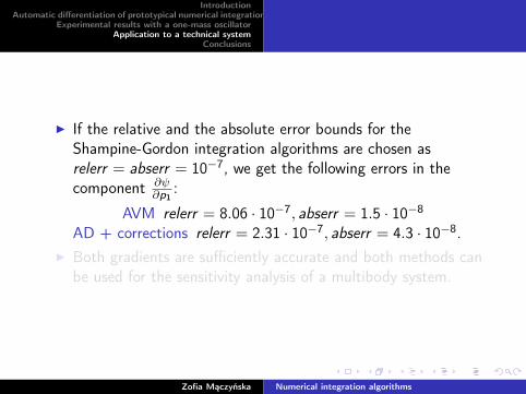
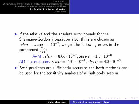
I If the relative and the absolute error bounds for theShampine-Gordon integration algorithms are chosen asrelerr = abserr = 10−7, we get the following errors in thecomponent ∂ψ
∂p1:
AVM relerr = 8.06 · 10−7, abserr = 1.5 · 10−8
AD + corrections relerr = 2.31 · 10−7, abserr = 4.3 · 10−8.I Both gradients are sufficiently accurate and both methods can
be used for the sensitivity analysis of a multibody system.
Zofia Mączyńska Numerical integration algorithms

IntroductionAutomatic differentiation of prototypical numerical integration algorithms
Experimental results with a one-mass oscillatorApplication to a technical system
Conclusions
I If the relative and the absolute error bounds for theShampine-Gordon integration algorithms are chosen asrelerr = abserr = 10−7, we get the following errors in thecomponent ∂ψ
∂p1:
AVM relerr = 8.06 · 10−7, abserr = 1.5 · 10−8
AD + corrections relerr = 2.31 · 10−7, abserr = 4.3 · 10−8.I Both gradients are sufficiently accurate and both methods can
be used for the sensitivity analysis of a multibody system.
Zofia Mączyńska Numerical integration algorithms

IntroductionAutomatic differentiation of prototypical numerical integration algorithms
Experimental results with a one-mass oscillatorApplication to a technical system
Conclusions
I In general:I the computation of the adjoint variable gradients is more
efficient, but they are based on a hand coded, highly optimizedalgorithm whose implementation took man-years
I AD-generated code is fairly simple to create and requires(including the result verification) much less time, at theexpense of a less efficient execution.
I However the time verification of the gradients can be very highand unless the algorithm and the implementations are wellunderstood, one should check the results carefully. This is dueto the fact that AD differentiate the algorithm without anyknowledge of the mathematics that underlie the algorithm.
Zofia Mączyńska Numerical integration algorithms

IntroductionAutomatic differentiation of prototypical numerical integration algorithms
Experimental results with a one-mass oscillatorApplication to a technical system
Conclusions
Conclusions
Zofia Mączyńska Numerical integration algorithms

IntroductionAutomatic differentiation of prototypical numerical integration algorithms
Experimental results with a one-mass oscillatorApplication to a technical system
Conclusions
I The numerical behavior of the criteria and the gradientcomputation must be studied carefully. It is not obvious thatthe stepsize control is determined only by the state variablesrequired for the criteria computation; and, therefore, the errorsintroduced in the state variables for the gradients may bebigger than the prescribed error bounds for the state variablesfor the criteria.
I The application of plan AD often yields the right resultsnevertheless the inclusion of expert knowledge can highlyimprove the performance and numerical behavior. (Example: ifthe differentiation of the stepsize control is switched off, wecan compute the correct gradients more efficiently)
Zofia Mączyńska Numerical integration algorithms


![Numerical Integration and Differentiation Quantitative ... · Numerical Integration and Di erentiation Quantitative Macroeconomics [Econ 5725] Raul Santaeul alia-Llopis Washington](https://static.fdocuments.us/doc/165x107/5b68494a7f8b9a6f778c9014/numerical-integration-and-differentiation-quantitative-numerical-integration.jpg)