A sensitivity analysis on the impact of regional trade ...

A sensitivity analysis on the impact / J. Ahcar-Olmos, D. Rodríguez-Barco 193Estudios de Economía. Vol. 47 - Nº 2, Diciembre 2020. Págs. 193-219

A sensitivity analysis on the impact of regional trade agreements in bilateral trade flows*1

Un análisis de sensibilidad sobre el impacto de los acuerdos comerciales regionales en los flujos bilaterales de comercio

2Jaime Ahcar-Olmos** 3David Rodríguez-Barco***

Abstract

We estimate the effect of RTAs on bilateral exports by means of a gravity model analyzing its sensitivity to different specifications and methods. RTAs generate a sizable positive effect. However, shifting to country-pair and time-varying fixed effects systematically reduces coefficients. Nevertheless, the RTA effect is consistent across methods and specifications.The RTA effect attributable to particular trade agreements displays high va-riability. While most RTAs increase trade, others present non-significant or negative results. We apply robustness checks to individual RTA estimates by presenting PPML time-invariant fixed effects and next to these, country-pair and time-varying fixed effects estimates. Thus, 38.2% of RTAs are positive and significant in both specifications. RTAs trade creation effects tend to prevail over trade diversion effects.

Key words: International Trade, Trade Liberalization, Regional Trade Agreements RTA, Gravity Model, Economic Integration.

JEL Classification: F13, F14, F15, F53, F55.

* The authors are grateful to the Editorial Board and two anonymous referees for their comments and corrections that greatly contributed to enhance the quality of this paper.

** [Corresponding author] Pontificia Universidad Javeriana-Cali. Faculty of Economics Sciences. Cali, Colombia. E-mail: [email protected]

*** Pontificia Universidad Javeriana-Cali. Faculty of Economics Sciences. Cali, Colombia. E-mail: [email protected]

Received: Novembre, 2019. Accepted: April, 2020.

Estudios de Economía, Vol. 47 - Nº 2194

Resumen

En este artículo estimamos, mediante un modelo de gravedad, el efecto de los Acuerdos Comerciales Regionales (ACR) en las exportaciones bilaterales, y realizamos un cuidadoso análisis de sensibilidad, considerando diferentes mé-todos y especificaciones. Los ACR presentan, por lo general, un efecto positivo considerable. Este impacto se reduce substancialmente al incluir efectos fijos país variables en el tiempo y efectos fijos individuales. No obstante, el efecto de los ACR es consistente a través de los métodos y especificaciones aplicados. Cuando el impacto de los ACR es calculado para cada acuerdo en particular, los coeficientes presentan una alta variabilidad. La mayoría de ACR presenta un impacto positivo. Otros presentan resultados no significativos o negativos. Para una mayor robustez de los resultados, los impactos de los ACR particulares fueron estimados con efectos fijos invariables en tiempo, y también con efectos fijos variables en el tiempo bajo el método de PPML. Así, el 38,2% de los ACR son positivos y significativos en ambas especificaciones. A su vez, los efectos de creación de comercio tienden a prevalecer sobre los efectos de desviación del comercio.

Palabras clave: Comercio Internacional, liberalización económica, Acuerdos Comerciales Regionales ACR, modelo de gravedad, integración económica.

Clasificación JEL: F13, F14, F15, F53, F55.

1. Introduction

After its creation in 1995, the World Trade Organization has been able to convince most of the countries to abide by the rules of multilateral trade. Nevertheless, its rounds of negotiations have come to a deadlock, partly ex-plained by the difficulty of making agreements among too many countries of a heterogeneous nature. In the midst of this, Regional Trade Agreements RTAs, appeared as a more effective way to close trade deals. They presented exponential growth from the 80s to the first decade of the current century, to slow down in recent years. The question, then, arises about its effectiveness.

Trump’s administration has dispensed with more than 70 years of liberal tradition in the United States, by dumping the Trans-Pacific Partnership (TPP) and the Transatlantic Trade and Investment Partnership (TTIP), the two most ambitions RTAs ever negotiated, while initiating a frontal trade war with China, and imposing duties on aluminium and steel worldwide. In the same direction, the United Kingdom has officially divorced from the most admired and profound RTA, the European Union. In a time where liberal ideas are under strain, answer-ing the question of whether RTAs really increase trade is even more important. Despite substantial progress to compute RTA estimates, the debate about the

A sensitivity analysis on the impact / J. Ahcar-Olmos, D. Rodríguez-Barco 195

effectiveness of RTAs remains open. The main objective of this paper is then to help answer the question: To what extent are RTAs able to create trade?

To do it, we employ the widely accepted approach of the gravity model. We build on the works of Baier and Bergstrand (2007), Martínez-Zarzoso et al. (2009); Kohl (2014) and Baier et al. (2019).

The main contribution of this paper is the presentation of a comprehensive sensitivity analysis based on a battery of relevant regression methods and speci-fications applied to the gravity equation on an updated database, providing the possibility of easy visualization and comparison, see Table 1. This information will also be valuable for future meta-analysis studies about the effect of RTAs on trade. We subsequently explore the RTA effect on bilateral trade for an ample sample of particular RTAs. Thus, coefficients for 123 particular RTAs comparing PPML time-invariant fixed effects (TIFE) and time-varying fixed effects (TVFE) estimates are presented in Table 3, which enables us to carry out robustness checks on their effectiveness. As far as we know, we are the first to present this comparison and analysis at disaggregated level for a large number of RTAs over a long period, see Table 4. Finally, we present results on trade creation and trade diversion for 25 relevant RTAs in Table 5.

Results from our most relevant specifications and methods point to a positive and significant effect of RTAs between 4.7% and 51.3% on bilateral exports. Considering particular RTAs, their impact is predominantly positive and significant. Trade creation effects in most of the cases offset trade diver-sion effects.

Gravity model estimations define what should be the normal pattern of trade, and then enable us to seek deviations from it, originated, for example, in the implementation of institutional arrangements. Given the counterfactual it offers, and its widespread use, the gravity model is tenable for calculating outcomes such as the expected gains from the entry into force of an RTA, or other institutional changes.

One important advantage of gravity models according to Bussière (2009) is that their results stem not only from a measure of multilateral trade integration (a country against all its trading partners), but also of bilateral trade integration (a country and each of its trading partners).

Our interest in finding the effects of RTAs in bilateral trade flows, hinges on the belief that higher international competition leads to greater productivity and higher cross-border exchanges increase wellbeing. We do not intend to disentangle this effect, although from Sachs et al. (1995), Wacziarg and Welch (2008) we have evidence that international trade promotes economic growth and then wellbeing. Similarly, Halpern et al. (2015) have established a positive relationship between firm import input access and productivity in the Hungarian economy, and Bas and Ledezma (2010) provided evidence of trade barriers reduction and with-in plant productivity increases in Chile.

In 1980, the GATT counted up to 83 signatories. In 2020 the number practically doubles, reaching 164 countries, now under the label of the WTO. Hayakawa and Kimura (2015) found that free trade agreements (FTAs) successfully reduce tariff


rates and non-tariff barriers (NTBs). Nevertheless, mixed effects were reported by Afesorgbor (2017), Caporale et al. (2012), Didia et al. (2015), Kahouli & Maktouf (2015), Martin-Mayoral et al. (2016) who studied the impact of RTAs on exports by trade blocs in different regions as the Americas, Africa or Europe. Their results maintain alive a long-standing debate on the optimal mechanism for liberalizing international trade, confronting the multilateral negotiation ap-proach to RTAs.

It is expected that membership to multilateral trade institutions would bear a strong positive effect on trade. Strong evidence for a positive WTO member-ship effect was found by Rose (2005), Subramanian and Wei (2007) and Kim (2011). Nevertheless, Eicher and Henn (2011) found evidence of an attenuated WTO membership impact after preferential trade agreements had entered into force. In view of the historical importance of this institution, this paper controls for country membership status in the WTO.

In parallel, the number of physical RTAs in force has steadily grown from 1980 to 2019. There were only 15 RTAs in 1980. They rose to 51 in 1995, 137 in 2005 to reach the number of 303 in 2019. Despite a slowdown in the number of new RTA negotiations worldwide, more RTAs are expected see the light in the years to come.

Special attention has been paid to Baier and Bergstrand (2007) who, using panel data on five years intervals, found that the average treatment effect of an RTA implies an increase of bilateral exports around 100% in 10 years. Another important contribution came from Magee (2008) who let the RTA dummy take leads and lags, thus finding significant anticipatory and slow motion impacts. Thus, in the long-run, an RTA increases trade on average by 89%. Regarding dynamics, Martínez et al., (2009), remark that bilateral exports are persistent and find significant effects for the lagged bilateral export flows, as well as for RTA coefficients at the disaggregated level.

RTA estimates have recently been reviewed downwards, a result that we confirm in this paper. This erosion effect was detected by De Sousa (2012) who focused on the effect of currency unions, and later by Kohl (2014) apply-ing the Baier and Bergstrand’s technique where he found that RTAs increased trade by at most 50%. Proving the reasons behind this behaviour goes beyond the scope of this paper. Yet, some hypothesis point out to the appearance of diminishing returns as more and more countries engage in RTAs; a rise in transaction costs coming from the multiplication of non-tariff measures such as rules of origin and local content requirements, or even a relaxation in the enforceability of existing RTAs due to a political movement of resistance to trade liberalization.

Following this introduction, the paper is organized as follows. Section 2 discusses methodological issues. Section 3 presents the data. Section 4 sets up the econometric specifications to be estimated. Section 5 presents and analyses results and section 6 concludes the paper.


2. Gravity model and methodology

Important advances in the micro-foundation of the gravity model are attributed to Anderson (1979) and Anderson and Van Wincoop (2003). They set up a model in which consumers maximize a homothetic Cobb-Douglas utility function that is identical in all countries; goods are differentiated by their country of origin, iceberg costs are assumed and only a fraction of the goods arrives at destination.

The mathematical approach developed by them puts multilateral resistance in the spotlight of the analysis. Their model takes us to estimate:

(1)

Where xij represents exports from country i to country j; yw, yi and yj represent

world, country i and country j’s GDPs, respectively; tij is a trade cost factor between i and j, consisting of geographical, political and institutional barriers. The parameter σ represents the elasticity of substitution between all goods and Pi and Pj are the multilateral resistance terms, which give us a measure of the relative openness of the economies. The Gravity equation is compatible with several underlying theories. A detailed discussion about the gravity model micro-foundation is available in Head and Mayer (2014).

Augmented gravity models control for confounders, which, if omitted, would bias the estimate of our parameter of interest on RTAs. Hence, we control for border contiguity and other cultural or institutional variables such as the use of a common language, Melitz and Toubal (2014), and colonial links, Head et al. (2010).

Anderson and van Wincoop (2003) pointed out the difficulties in estimating unbiased coefficients through cross-sections as well as the threat of omitted vari-able bias derived from multilateral resistance. Thus, Panel data models enabling for fixed effects specifications provided a solution to the fact that Pi and Pj, the so-called multilateral resistance terms in equation (1) are unobservable and the procedure to estimate them implies a non-linear routine. De Benedictis and Taglioni (2011) examine the sensitivity of OLS estimates to variations in fixed effects. These procedures control for endogeneity from unobservable heterogene-ity and then for omitted variable bias derived from multilateral resistance. The authors consider the introduction of time-varying fixed effects for importing and exporting countries a robust solution.

Apart from the multilateral resistance difficulty, the possibility of endogene-ity between bilateral trade and institutional trade liberalization variables is also prominent. Trefler (1993) pointed out that a country’s decision to sign a regional trade agreement could not be completely exogenous. In the same way, Ghosh and Yamarik (2004) based on extreme bounds analysis showed that the RTAs coefficient computed with cross-sectional data could be biased in the presence of endogeneity and Baldwin and Jaimovich (2012) found that free trade agreements


could be contagious (domino effect). When endogeneity is present, traditional estimation methods could result in inconsistent estimates. Instrumental variable methods can deal with endogeneity, allowing for stronger causal claims.

In that vein, Baier and Bergstrand (2007, 92) stated “standard cross-section techniques using instrumental variables and control functions do not provide stable estimates of RTA average treatment effect in the presence of endogeneity, and tests of over-identifying restrictions generally fail”. They suggested that panel data methodologies must be implemented to estimate the RTA coefficient.

A panel approach will then be preferred over cross-section because it ac-counts better for country observed and unobserved time-varying or time-invariant heterogeneity. It provides the possibility of controlling for relevant relationships over time, avoiding the risk of choosing an unrepresentative year Antonucci and Manzocchi (2006). Panels also improve the efficiency of the estimates, Cheng Hsiao (2003). The panel structure would deal relatively well with the endogeneity problem considering that the reasons linked to RTAs not being exogenous should most probably be related to time-invariant heterogeneity (huge pre-existing trade flows, or contiguity).

Not all RTAs are equal. Dür et al. (2014) created deep integration indica-tors proving that differences on the depth of the agreements produces weaker effects for shallow agreements. Considering the heterogeneity of economic integration agreements, Egger and Nigai (2015) concluded that shifting to deeper trade agreement increases welfare, this effect being particularly high for some countries. Kohl et al. (2016); Ahcar and Siroën (2017) confirmed the effects of deep integration on trade, where deeper agreements result in larger gains. Baier et al. (2018) also found that certain integration settings produce greater impacts on the intensive margin than on the extensive margin.

Seeking better predictions of the effect of new economic integration agree-ments, Baier et al. (2018) and Baier et al. (2019) went beyond the importance of accounting for RTA heterogeneity. They found asymmetries in the RTA effect linked to the direction of trade. They also proved that country-pair heterogene-ity is relevant as any given integration agreement can produce different effects on trade. For example, partners engaged in pre-existing economic integration agreements and distant pairs of countries obtain weaker gains out of further integration.

Considering that the main objective of this paper is to compare the average effect of an RTA through different specifications and methods, we want to make the caveat that not all RTA are equally designed. Hence, we do not expect to interpret these coefficients as precise predictions of the effect of any new RTA agreement, as literature acknowledges that information on RTA heterogeneity is required for accurate forecasting purposes. Nevertheless, to mitigate these shortcomings, we estimate the RTA effect for particular couples and blocks, where we can observe a long range of variability on the effect of RTA, possibly caused by this heterogeneity.


3. Data

To deal with the challenges mentioned above and to successfully estimate our variables of interest, this research set up an exhaustive data set to run a gravity model. It consists of bilateral trade flows for 153 countries from 1980 to 2018 that add up to 715.626 individual bilateral trade flows and an extensive set of control variables.

Bilateral Exports are taken in current dollars at fob values from the International Monetary Fund (IMF) Direction of Trade Statistics Database DOTS (2020). The current GDP in dollars, population in number of inhabitants and urban participation in percentages are provided by the World Development Indicators (WDI) database of the World Bank (2020). The surface in square meters as well as island and landlocked status were constructed by the author based on data from the World Factbook of the Central Intelligence Agency of the United States of America CIA (2020). Weighted distance in Km, common land border and colonial links stem from the CEPII (2013): Head et al. (2010) Gravity dataset.

The dummy variable for Regional Trade Agreements was constructed by the author based on the Regional Trade Agreements Information System (RTA-IS) of the World Trade Organization WTO (2020), and from de Sousa RTA data set for De Sousa (2012). Generalized System of Preferences GSP is built by the author based on the Database on Preferential Trade Arrangements of the World Trade Organization WTO (2020). The author based on the World Trade Organization WTO information (2020) constructed GATT membership and OECD membership based on information from the Organisation for Economic Co-operation and Development (OECD) (2020).

4. Econometric specifications

The equation to estimate with OLS, with time-fixed effects and exporter and importer time-invariant fixed effects is presented in (2) below:

(2)

Where, the dependent variable lnXijt represents the natural logarithm of current dollar fob export values from country i to country j; β1 is the RTA coefficient, our parameter of interest; β0 is a constant term, αt represents the time-fixed effects, αi represents time-invariant exporter fixed effects, αj are the importer time-invariant fixed effects and εijt is an idiosyncratic error term.

Likewise, Sit and Mjt are vectors of time-varying monadic controls for ex-porters and importers respectively composed of h variables: lnGDPit, lnpopit, urpartit, OECDit and GATTit, gspproviderit, gspbenit as well as, lnGDPjt, lnpopjt, urparjt, OECDjt and GATTjt.

Here, ψ and φ are vectors of coefficients to be estimated concerning the above control variables, and the subscript h indicates variables.


We define lnGDPit and lnGDPjt as the natural logarithms for current dollar GDPs from countries i and j; lnpopit, lnpopjt are natural logarithms for the popula-tion in number of inhabitants of countries i and j; urpartit and urpartjt stand for the percentage of urban population in country i and j respectively; this could be seen as a measure of the degree of development of countries, as more developed countries tend to be relatively more urbanized.

Other non-dyadic variables attempt to control for institutional traits related to commerce; these are gattit and gattjt that take on 1 if countries i/j belong to the GATT/WTO respectively. We use variable gspbenit that takes on 1 if country i is receiving the generalized system of preferences or any other unilateral prefer-ence scheme from country j, otherwise 0; gspproviderit takes on 1 if country i is granting the generalized system of preferences or any other unilateral preference scheme to country j; oecdit and oecdjt take on 1 if the countries i/j belong to the Organization of Economic Cooperation and Development OECD.

When no country fixed effects are introduced, controlling for time-invariant monadic variables such as the total surface of a country, the fact of being an island or being landlocked, helps to improve results. Then, vectors Sit and Mit are augmented with variables lnareait, islit and landlockedit; and lnareajt, isljt and landlockedjt respectively. Here, lnareait and lnareajt are the natural logarithms for the surface in square km of country i and j; Isl takes on 1 if country i/j is an island, otherwise 0; and landlocked takes on 1 if country i/j is deprived of a direct access to the sea, otherwise 0.

Finally, Zijt is a vector of dyadic variables that helps to minimize possible bias, composed of g variables: contgijt, comlangijt, col45ijt and lndistijt and ϕ is a vector of coefficients to be estimated concerning these dyadic variables; the subscript g is to indicate variables, where lndistijt is the natural logarithm for the weighted distance between countries i and j; contigijt takes on 1 if there is a common land frontier between i and j, otherwise 0; comlangijt takes on 1 if at least 9% of the pair population share the same language, otherwise 0; col45ijt takes on 1 if both countries were under a colonial relationship before 1945, otherwise 0; and finally our variable of interest rtaijt takes on 1 if both countries share a free trade agreement, otherwise 0.

The equation to be estimated with random effects or with country-pair fixed effects is presented in (3) below. Here we follow (4) assumption.

(3)

(4)

Where EV stands for explanatory variables, (ij) represents the entities, t represents years, and g is to enumerate the explanatory variables.

αij represents country-pair fixed effect. For the traditional fixed effect model (within transformation) (4) assumption is modified to allow for a differential intercept for each country pair ij, then, a correlation between at least some of


the explanatory variables and the country-pair fixed effects is permitted. See (5). This method does not allow controlling for time-invariant exporter and importer fixed effects at the same time, as the pair-fixed effects are collinear with country fixed effects. Thus, all time-invariant variables are dropped by the within transformation, Greene (2011).

(5)

Increasing acceptance to estimate gravity models is acknowledged to the Poisson Pseudo Maximum Likelihood estimator. This technique has been defended by Santos Silva and Tenreyro (2006; 2011) and Fally (2015) as the more reliable method to estimate the gravity equation because it deals with heteroscedasticity problems better than traditional OLS methods. Furthermore, in their work of 2011, they presented further evidence that the PPML estimator generates consistent estimates, even in the presence of a large number of zero values in the data set, a recurrent difficulty in gravity models.

(6) presents the PPML specification when we introduce year fixed effects and exporter and importer time-invariant fixed effects:

(6)

Here, Xijt represents the value of the fob merchandise exports from country i to country j in current dollars and uijt = exp ((1 – σ) εijt). We chose this specifica-tion to evaluate trade diversion for a set of interesting RTAs. Thus we introduce a vector of RTAit trade diversion dummies next to their associated vector of RTAijt. The subscript k stands for the number of RTA dummies included. (6) can now be read as:

(7)

Below in (8) we relax the assumption of the maintenance of unchanging gaps among different intercepts, or stable tendencies, through time. The inclusion of time-varying country fixed effects in the PPML specification leads us to estimate.

(8)

Where αit stands for time varying exporter fixed effects and αjt are the im-porter time-varying fixed effects. In (9) we include country-pair fixed effects in a specification that not only control for time varying unobserved heterogeneity at the country level but also for time invariant unobserved heterogeneity at the individual level. This is the literature preferred specification.

(9)


Improvements in Stata procedures documented by Correia et al. (2019) and Larch et al. (2019) have made possible the estimation of models with larger number of fixed effects with the PPML estimator, such as those presented in equations (8) and (9).

5. Results

In accordance with Baldwin and Taglioni (2006) this paper includes specifica-tions that control for the passing of time using time-fixed effects. This approach allows us to work properly with GDP dollars, avoiding the so-called bronze medal mistake, which occurs when deflating these time series to obtain their real values. Non-averaged bilateral trade data to avoid the silver medal mistake is also used. The inclusion of time-invariant country fixed effects permits the partial offsetting of the endogeneity problem caused by omitted variables, in what is known as the gold medal mistake.

Under the OLS and PPML method, this paper also controls for time-varying country fixed effects for importers and exporters. This procedure would furnish a robust estimate of RTAs that controls for multilateral resistant and other omit-ted variables that change with the passing of time. The summary of the results will be presented in Table 1 to make comparison easier.

5.1. Traditional methods of estimation

5.1.1. Pooled ols specifications results

In its first row, Table 1 presents results based on the pooled OLS specifica-tions. An analysis of the RTA coefficients shows that the model with no fixed effects in column 1 estimates a rise of 39.0%, (e0.329 -1) in bilateral exports affected by RTAs relative to flows not influenced by them. It underestimates the impact of RTAs on international bilateral trade with respect to other OLS models that control for fixed effects, excepting for model 8 which simultanusly control for TVFE and country-pair fixed effects. This specficiation indicates a rise of 28.5% in bilateral trade.

When only time-fixed effects are controlled for, model 2 on the pooled OLS specification, the RTA coefficient overreacts, see column 2 of Table 1, producing a rise of 104.6% in bilateral exports affected by a RTA with respect to bilateral trade not affected by RTAs. This is the highest global RTA estimate computed in this paper.

5.1.2. Random effects and country-pair fixed effects results

A random effects model assumes that unobserved individual effects are uncorrelated with the explanatory variables Wooldridge (2012). The random effects model moves RTA estimates downward with respect to pooled OLS, yet a positive and significant effect is persistent.


The RTA random effects estimates in model 6 (see column 6 and random effects row) imply a slightly less important increase in trade than the model 2, controlling for time-fixed effects but omitting time-invariant fixed effects. Thus, when time-fixed effects and exporter and importer time-invariant fixed effects are introduced together as in model 6, we obtain an increase of about 31.3% in bilateral exports. To distinguish which model performs better between OLS and random effects we applied Breusch and Pagan (1980) test that checks if random effects are present. Based on their Lagrangian multiplier test for random effects, the OLS pooled model is outperformed by the random effects model.

When we relax the assumption that country-pair individuals’ effects are uncorrelated with covariates, we obtain a fixed effect model. This model creates fixed effects for each bilateral export flow that remains invariant through time. Thus, observed and unobserved time-invariant heterogeneity at the country-pair level is kept at bay.

The fixed effects model in column 3 of the Fixed Effects row estimates that bilateral exports sharing a RTA increase by 19.1%, relative to flows without RTAs. Introducing time fixed effects to this model results in an increase of 18.9% in bilateral trade.

Results from the Hausman’s specification test, establish that the fixed effect model fits better than the random effects. Particularities at individual level are then correlated with the explanatory variables. Nevertheless, the fixed effect regression at the individual country-pair level generates estimates that could be underestimating the RTA effect on bilateral trade, particularly when time fixed effects are accounted for.

5.2. Current methods of estimation

5.2.1. PPML specification results

The PPLM seems to be the more reliable method to estimate the gravity model. Martínez-Zarzoso (2013) validates this method through a series of Monte Carlo experiments. Fally (2015), Montenegro et al. (2011) and Martín-Montaner et al. (2014) gives additional support to PPML estimations over another techniques.

In the specification without time-fixed effects or country fixed effects, Column 1 in Table 1, the PPML estimate of RTA presents a rise of 10.5%. The introduction of time-fixed effects and country time-invariant fixed effects cor-rects PPML estimates upwards.

Likewise, PPML estimations shift upward to the introduction of time-varying fixed effects for exporter and importer countries, see column 7. The coefficient is lower in the TIFE and time-fixed specification, column 6, than in column 7, by 0.074 points, equivalent to 10.8 percentage points, which is a relevant dif-ference that deserves attention. The TIFE and time-fixed effect model estimated by PPML produces an increase of 40.5% in bilateral exports affected by a RTA, compared with bilateral export flows that do not profit from any RTA; the com-parable result using TVFE estimated by PPML is 51.3%.


We observe a sharp reduction of the RTA estimate when using PPML con-trolling simultaneously for TVFE and country-pair fixed effects, see column 8. This behaviour is also present under the OLS method, but PPML accentuates the decline. Sharing an RTA will only increase trade by around 4.7% in this specification, which is the preferred approach in literature.

5.2.2. The Baier and Bergstrand method

The Baier and Bergstrand technique consists of controlling for multilateral resistance and RTA endogeneity by the means of introducing country-pair fixed effects and time varying fixed-effects on a panel of non-successive years that we call periods. In accordance with Baier and Bergstrand we estimated our model keeping 10 periods, so we retain information for intervals of four years. Baier and Bergstrand (2007) kept data for intervals of five years1. In model 8 of the Baier and Bergstrand specification where country-pair and time-varying country fixed effects are computed together, the introduction of a RTA will increase bilateral exports by around 30.0% for OLS and 3.9% for PPML. RTA estimates under the Baier and Bergstrand method, where country fixed effects are accounted for; present higher values compared with those including country-pair fixed effects specifications. See Table 1.

The Baier and Bergstrand method simplifies the analysis of the dynamics of RTA through time. Variable rtaijt-1 and rtaijt-2 will capture the impact of RTAs on bilateral exports four and eight years before their entry into force or phase-in effects. It also enables the evaluation of anticipatory effects. Thus, rtaijt+1 de-scribes the effects of the announcement and pre-entry into force of RTAs. Table 2 presents results for OLS and PPML regressions based on the time varying fixed effects and country-pair fixed effects specification.

Using the Baier and Bergstrand method with OLS, the first lag of the RTAs is positive and significant, but this does not hold for PPML specifications. Introducing a second lag in the specification drops the significance of the first lag. Using OLS, the RTAs effect experience a cumulative increase of 30.5% in bilateral exports during the first four year of entry into force, and approximately a 32.3% cumulative effect during the eight first years. The four years prior to its entry into force, known as the anticipatory effect of RTAs, is non-significant, which suggest strict exogeneity of RTAs, mitigating doubts about reversal cau-sality where an increase in trade could cause RTA appearance. Estimates using PPML show an absence of cumulative and anticipatory effects. See columns (5-8) in Table 2.

1 The results we show are estimated with data for years 1980, 1984, 1988, 1992, 1996, 2000, 2004, 2008, 2012 and 2016.


5.3. Instrumental variable methods and dynamics

5.3.1. The Hausman and Taylor instrumental variable estimator

To deal with RTA endogeneity problem of the type suggested by Baldwin and Jaimovich (2012) where a new free trade agreement between A and B increases the probability that C will sign a RTA with A or B or due to pre-existing overtrad-ing patterns raised by Baier and Bergstrand (2007), we resort to the Hausman and Taylor estimator. These authors have proposed an instrumental variables estimator that uses only the information within the model by taking deviations from group means that can be used as instrumental variables. (Greene, 2011). The correct use of instrumental variable methods requires data on a sufficient number of instruments that are both exogenous and relevant. Swamy et al. (2015) argue that such instruments, weak or strong, are often impossible to find.

The Hausman-Taylor estimator assumes that some of the explanatory vari-ables are correlated with the individual-level random effect αij, while none of the explanatory variables are correlated with the idiosyncratic error εijt. In addition to standard assumptions, we also assume that RTA was the only endogenous variable in the model. Through Monte Carlo simulations, this estimator has proved to be robust for endogenous time-varying variables in large sample and perfect knowledge gravity model frameworks. (Mitze, 2010).

H-T estimates of RTA indicate an increase in bilateral trade between 18.2% and 30.2%. We should take these estimates with prudence as the Hausman test applied indicate that we should prefer the fixed effects estimator over the Hausman and Taylor estimator. Nevertheless, being the Hausman and Taylor estimator an instrumental variable estimator we should gain some confidence on making causal claims about the RTA effect.

Other instrumental variable techniques were also considered. The instru-mental variable fixed effects and random effects estimators were computed using as instruments for RTA its lags on t-3 and t-4, under the assumption that these variables only influence bilateral exports by the influence they exert on the variable of interest RTA. Results suggest an upward bias for RTA in the IV-Dynamics using the third and fourth lags of the RTA, compared to H-T estimates.

5.3.2. GMM regression and the Arellano and Bond estimator

The main purpose of the Arellano and Bond (1991) method is to consistently estimate the dependent variable lags. This technique also allows setting other explanatory variables as endogenous by using GMM-type instruments to com-pute the causal effects of endogenous covariates. We tried to take advantage of this possibility and intended to use it to correct a possible endogeneity bias on the RTA estimates, nevertheless the Sargan test and the Hansen test failed, sug-gesting that lagged RTA instruments and lagged bilateral exports instruments were not valid because of overidentification.


TAB

LE

1R

TA E

STIM

AT

ES

SUM

MA

RY

Fixe

d E

ffec

ts C

ontr

ols

(1)

(2)

(3)

(4)

(5)

(6)

(7)

(9)

Tim

e in

vari

ant E

xpor

ter

Fixe

d E

ffec

tsN

ON

ON

ON

OY

ES

YE

SN

ON

OT

ime

inva

rian

t Im

port

er F

ixed

Eff

ects

NO

NO

NO

NO

YE

SY

ES

NO

NO

Tim

e V

aryi

ng E

xpor

ter

Fixe

d E

ffec

tsN

ON

ON

ON

ON

ON

OY

ES

YE

ST

ime

Var

ying

Im

port

er F

ixed

Eff

ects

NO

NO

NO

NO

NO

NO

YE

SY

ES

Cou

ntry

-pai

r Fi

xed

Eff

ects

NO

NO

YE

SY

ES

NO

NO

NO

YE

ST

ime

Fixe

d E

ffec

tsN

OY

ES

NO

YE

SN

OY

ES

NO

NO

Eco

nom

etri

c M

etho

d

Pool

ed O

LS

0.32

9***

0.71

6***

0.59

1***

0.63

1***

0.67

9***

0.25

1***

Ran

dom

Eff

ects

0.16

4***

0.29

6***

0.21

0***

0.27

2***

Fixe

d E

ffec

ts (

with

in)

0.17

5***

0.

173*

**

PPM

L0.

100*

**0.

257*

**0.

067*

**0.

080*

**0.

336*

**0.

340*

**0.

414*

**0.

046*

**

Bai

er a

nd B

ergs

tran

d (O

LS)

0.14

8***

0.36

2***

0.17

0***

0.22

5***

0.60

7***

0.64

4***

0.70

6***

0.26

2***

Bai

er a

nd B

ergs

tran

d (P

PML

)0.

086*

*0.

251*

**0.

041*

0.06

6***

0.33

0***

0.33

9***

0.41

0***

0.03

8**

IV: H

ausm

an a

nd T

aylo

r0.

167*

**0.

264*

*0.

183*

**0.

246*

** IV

-Dyn

amic

s: R

TA la

gs 3

and

40.

268*

**0.

473*

**0.

304*

**0.

402*

**0.

356*

**0.

451*

** IV

-Dyn

amic

s: A

rella

no-B

ond

(GM

M)

-0.2

47**

0.49

3***

Not

e: *

** p

<0.

01, *

* p<

0.05

, * p

<0.

1. R

obus

t sta

ndar

d er

rors

.So

urce

: Ela

bora

ted

by th

e au

thor

s.


TAB

LE

2D

YN

AM

ICS

BA

IER

AN

D B

ER

GST

RA

ND

RE

GR

ESS

ION

ON

153

CO

UN

TR

IES

FOR

10

PER

IOD

S FR

OM

198

0 T

O 2

016.

OL

S A

ND

PPM

L E

STIM

AT

OR

S

(1

)ln

xijt

(2)

lnxi

jt(3

)ln

xijt

(4)

lnxi

jt(5

)X

ijt

(6)

Xij

t(7

)X

ijt

(8)

Xij

t

rtai

jt 0.

251*

**0.

061*

**0.

059*

**0.

079*

**0.

046*

*0.

023

0.02

00.

022

rtai

jt-1

0.20

5***

-0.0

190.

009

0.01

9–0

.002

0.00

2

rtai

jt-2

0.24

0***

0.23

6***

–0.0

210.

021

rtai

jt+1

–0.0

21–0

.009

Con

stan

t15

.323

***

15.3

31**

*15

.340

***

15.3

52**

*4.

837*

**4.

850*

**4.

865*

**4.

838*

**

Obs

erva

tions

126,

441

115,

169

103,

085

84,2

7110

3,58

391

,237

79,0

8763

,654

R-s

quar

ed0.

878

0.88

50.

892

0.90

20.

957

0.95

80.

960

0.95

9

Not

e: *

** p

<0.

01, *

* p<

0.05

, * p

<0.

1. R

obus

t sta

ndar

d er

rors

. All

estim

atio

ns in

clud

ed c

ount

ry-p

air

and

time

vary

ing

expo

rter

and

tim

e va

ryin

g im

port

er f

ixed

eff

ects

. C

olum

ns 1

-4 f

or O

LS.

Col

umns

5-8

for

PPM

L.

Sour

ce: E

labo

rate

d by

the

auth

ors.


Among the techniques and methods applied in this paper, Arellano Bond specifications are the only ones to produce a significant and negative effect for the RTA dummy, although it disappears after dummy year inclusion. We pres-ent the Arellano-Bond RTA results in Table 1, assuming the RTA dummy as an exogenous variable and using the dependent variable lags as instruments to correct for the endogeneity of the first lag of the bilateral exports.

The results reported in Table 1 for Arellano-Bond RTA coefficients come from a regression that uses the first lag of the dependent variable as a regressor to account for the dynamics of the model, and all available dependent variable lags as instruments for this. In column 1 we show the result for the equation without year fixed effects, and in column 2 we control with time dummies. For robustness, we verified that the RTA coefficient is systematically negative in the regressions with no year effects as we reduce the number of lagged instruments, and overidentification problems also persist.

These results could be interpreted as evidence of the static approach strength over the dynamic approach, and also as an invitation for further research on dynamics of the dependent variable and RTAs. Some interesting works on dynamics for international trade gravity models can be found in Caporale et al. (2012), Didia et al. (2015) and Kahouli & Maktouf, (2015).

5.4. RTA estimates summary

Table 1 summarizes RTA estimates results, taking into account the econometric method and the fixed effect mix introduced. The methods used include pooled regression, random effects, fixed effects (within), PPML, Baier and Bergstrand for OLS and for PPML, Hausman and Taylor, Instrumental variables and dy-namics models. Thus, in static models, the RTA coefficient is always positive and significant. Depending on the method and specification employed, statics models coefficients can vary from an estimate 0.038 in the Baier and Bergstrand-PPML method with TVFE and country-pair fixed effects, to levels as high as 0.716 that comes from the OLS pooled regression using only time fixed effects.

5.5. RTAs effects at the disaggregated level

The effect of particular RTAs computed by means of dummy variables for each scheme such as EU, NAFTA or MERCOSUR has been reviewed in Magee (2008), Eicher and Henn (2011) and Kohl (2014), Baier and Bergstrand (2019) among others.

Most of the preceding studies on the effects of particular RTAs are estimated by OLS techniques. This paper offers 123 RTA estimates based on PPML over a database across 153 countries and observations from 1980 to 2018, see Table 3. We apply a robustness check to our individual RTAs estimates by presenting PPML time-invariant fixed effects and next to them time-varying fixed effects estimates. On the time-invariant country fixed effects specification, we control for RTA membership other than the RTA of interest, distance between countries


TABLE 3PPML ESTIMATES FOR A GROUP OF 123 REGIONAL TRADE AGREEMENTS FROM A

153 COUNTRIES 1980-2018 DATA SET

Agreement Year(1) TIFE (2) TVFE

Agreement Year(1) TIFE (2) TVFE

RTA coef. RTA coef. RTA coef. RTA coef.

ASEAN free trade area 1992 0.165*** –0.211*** EC–Jordan 2002 –0.279*** –0.237***ASEAN-Australia 2010 0.352*** 0.028 EC–Lebanon 2003 0.366*** –0.249***ASEAN-India 2010 0.242*** 0.009 EC–Mexico 2000 –0.161*** –0.204***ASEAN-Korea 2010 0.799*** 0.156*** EC–Moldova 2015 0.322** 0.229***ASEAN-New Zealand 2010 0.402*** 0.348*** EC–Morocco 2000 0.763*** 0.149***Australia-Japan 2015 0.652*** 0.218*** ECOWAS 1993 1.041*** 0.697***Australia-Korea 2015 0.758*** 0.111 EC–Peru 2012 0.224*** –0.044Australia-New Zealand 1983 1.269*** 0.486*** EC–South Africa 2000 0.485*** –0.446***Australia-Singapore 2003 0.274*** 0.135** EC–Syria 1977 0.515*** –1.139***Australia-Thailand 2005 0.777* 0.483*** EC–Tunisia 1998 0.913*** –0.003CAN (Andean Community)

1988 0.928*** 0.956*** EC–Turkey 1996 0.462*** 0.106***

Canada Colombia 2012 –0.524*** –0.104 Ecuador–EC 2017 –0.006 0.139**Canada-EC 2018 –0.236** 0.163*** EFTA–Israel 1993 0.354*** –0.599***Canada-EFTA 2009 0.226** –0.261*** EFTA–Korea 2006 0.437*** –0.009Canada-Jordan 2013 –0.805*** 0.563*** EFTA–Peru 2012 1.574*** –0.016Canada-Peru 2009 0.857*** 0.487*** GCC 2003 –0.812*** 0.032CEFTA 2007 0.389*** 0.181*** Group of Three 1995 0.504*** 0.895***Chile Colombia1 1994 0.905*** –0.025 India–Japan 2011 –0.685*** –0.140***Chile Colombia2 2009 0.924*** 0.106 India–Malaysia 2011 0.436*** –0.029Chile-Australia 2009 –0.852*** 0.524*** India–Singapore 2005 0.300*** –0.053Chile-China 2006 1.494*** 0.606*** India–Sri Lanka 2001 1.251*** 0.532***Chile-EC 2003 0.201*** –0.247*** Japan–ASEAN 2008 0.581*** 0.108***Chile-India 2008 0.669*** –0.021 Japan–Indonesia 2008 0.648*** –0.111***Chile-Japan 2007 0.867*** 0.274*** Japan–Malaysia 2006 0.661*** 0.121***Chile-Korea 2004 1.579*** 0.246*** Japan–Mexico 2005 –0.099 0.034Chile-Malaysia 2012 –0.919*** 0.035 Japan–Mongolia 2016 –0.355 0.736***Chile-Peru1 1999 0.819*** 0.250*** Japan–Peru 2012 0.318** 0.056Chile-Peru2 2009 0.657*** –0.292*** Japan–Philippines 2008 0.507*** 0.294***Chile-Thailand 2015 0.120 0.333*** Japan–Singapore 2002 0.250*** 0.084**Chile-Turkey 2011 –0.297*** 0.209** Japan–Switzerland 2009 0.654*** 0.100 Chile-Vietnam 2014 0.719*** 0.431*** Japan–Thailand 2007 0.885*** 0.237***China-ASEAN 2005 –0.160*** 0.146*** Japan–Vietnam 2009 0.636*** –0.050China-Costa Rica 2012 0.075 0.229 Korea Republic–Canada 2015 –0.033 –0.039China-New Zealand 2008 0.188* 0.506*** Korea Republic–India 2010 0.058 –0.023China-Pakistan 2007 –0.096 0.181*** Korea Republic–New Zealand 2016 0.156*** 0.030China-Peru 2010 1.351*** 0.339*** Korea Rep.–Singapore 2006 0.649*** 0.300***China-Singapore 2009 –0.256*** –0.025 Korea Republic–Turkey 2013 0.424*** 0.301***CIS 1994 1.561*** 0.020 Korea–Peru 2012 1.292*** 0.348***COL (CAN) MERCOSUR 2005 –0.006 0.247*** Mauricio–Turkey 2013 0.865*** 0.833***Colombia Northern Triangle

2009 0.514*** 0.489*** MERCOSUR 1991 1.139*** 0.592***

Colombia-Costa Rica 2017 –0.257 –0.220* MERCOSUR–India 2009 0.325*** 0.206**Colombia-EC 2013 0.185** –0.0317 Mercosur–Peru 2006 0.024 –0.105**Colombia-EFTA 2011 0.345** –0.396*** NAFTA 1994 0.871*** 0.439***Colombia-Korea 2017 0.369*** 0.036 PAFTA 1998 –0.699*** 0.547***COMESA 1994 1.273*** 1.067*** SAFTA 2006 0.284** –0.041EAEC 1997 1.155*** 0.417*** Southern African Develop.

Comm.2000 1.992*** 0.229***

EC Enlargement (10) 1981 0.239*** 0.018 Turkey–EFTA 1992 0.031 –0.268***EC Enlargement (12) 1986 0.259*** 0.106*** Ukraine–Belarus 2006 1.658*** 0.519***EC Enlargement (15) 1995 0.309*** 0.083*** Ukraine–Kazakhstan 1998 1.864*** 0.188EC Enlargement (25) 2004 0.277*** 0.086*** Ukraine–Turkmenistan 1995 3.266*** 0.366EC Enlargement (27) 2007 0.496*** 0.143*** US–Australia 2005 –0.781*** –0.237***EC Enlargement (28) 2013 0.534*** 0.076*** US–Bahrain 2006 –0.163 0.089EC-Albania 2006 0.976*** –0.031 US–CAFTA–DR 2006 0.477*** 0.132***EC-Algeria 2005 0.262*** –0.227*** US–Chile 2004 –0.228** 0.324***EC-Cameroon 2009 0.433*** –0.464*** US–Colombia 2012 0.153** 0.026EC-Caricom 2008 –0.623*** –0.122*** US–Israel 1985 1.093*** 0.253***EC-Côte d’Ivoire 2009 0.275*** –0.283*** US–Jordan 2001 0.339*** 0.778***EC-Croatia 2002 0.803*** –0.130*** US–Morocco 2006 –0.716*** 0.367***EC-EFTA 1973 0.220*** –0.082*** US–Oman 2009 –0.703*** 0.302***EC-Egypt 2004 0.185*** –0.342*** US–Peru 2009 –0.147 0.096**EC-Ghana 2017 –0.416 –0.472*** US–Singapore 2004 –0.021 –0.273***EC-Israel 2000 0.042 –0.283***

Source: Elaborated by the author. *** p<0.01, ** p<0.05, * p<0.1. Robust standard errors. Note: Columns (1) are estimated with time-invariant fixed effects and time fixed effects. Columns (2) include

time-varying fixed effects and country-pair fixed effects.


i and j, common land frontier between i and j, if the country-pair shares the same language, and if both countries were under a colonial relationship before 1945. Profiting from recent PPML computing power improvements, Correia et al (2019), we respectively estimate PPML country-pair and time-varying fixed effects for individual RTAs. This is one of the major contributions of this paper.

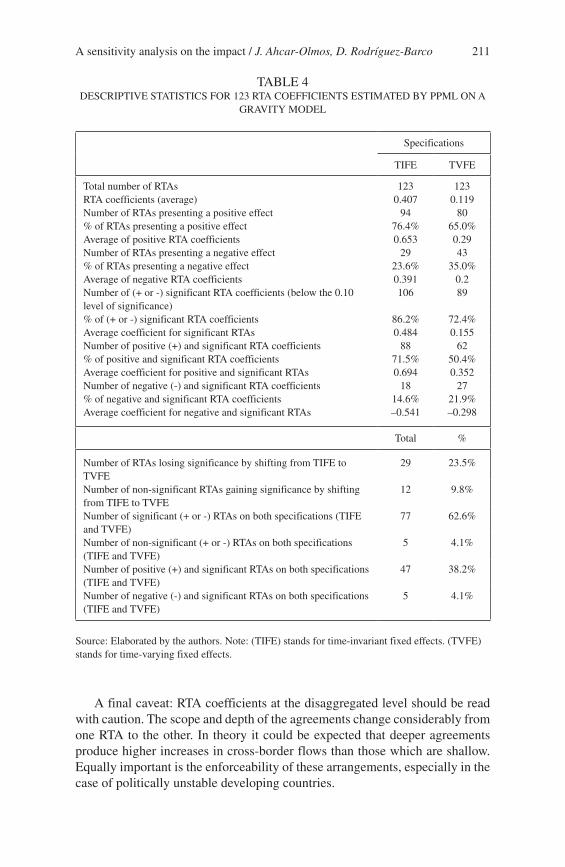
As can be seen in Table 4, column 1, most of the RTA estimates, 94 out of the 123, equivalent to 76.4% of the sample, show a positive sign. Column 2, gives a less optimistic view, presenting 80 positive estimates. In addition, 62 RTA estimates bear out positive signs in both specifications, and 47, equiva-lent to 38.2% are positive and significant in both PPML specifications. These results, point to a larger proportion of trade agreements that are successful in promoting trade than in Kohl (2014), who reported that only 44 out of 166 RTAs, equivalent to 26.5% of their sample presented a positive and significant effect. Another interesting comparison is Baier et al. (2019) who used a sample of 65 RTAs and found positive statically significant effects for the majority of the agreements, 54%. Nevertheless, their results are not strictly comparable to ours, as they account for the effect of lagged RTAs.

The median RTA on this sample increases trade by 42.2%, (e0.352 – 1). Despite the dispersion, around 75.6% of RTA’s estimates fall within one standard devia-tion of this median effect and 93.5% within two standard deviations.

Some straightforward outliers are the Chile-Malaysia, Gulf Council Countries GCC, PAFTA and EC-Caricom agreements, which seem to be highly coun-terproductive to trade creation, while the largest positive effects are posted by Ukraine-Turkmenistan, SADC, the Chile-Korea, EFTA-Peru and the Ukraine-Kazakhstan agreement. The latest impressive results of these cases concern former Soviet Union countries and could be attributed to some kind of transition effect or measurement error that could bias their estimates upward. Chile-Malaysia and GCC, Ukraine-Turkmenistan, EFTA-Peru and Ukraine-Kazakhstan become non-significant under the TVFE and country-pair specification. As we can observe in Table 4, around 23% of the RTA lose significance when shifting from TIFE to TVFE. The number of agreements significant in both specifications is 77, equivalent to 63%. One intriguing result is that only 50.4% of RTAs are positive and significant under the country-pair and TVFE specification. That number is substantially higher under the TIFE specification reaching 71.5% of RTAs.

Considering results in both specifications, United States agreements present mixed results, showing trade creation with Israel, Jordan and Colombia while the agreement with Bahrein is non-significant. Counterproductive effects appear with Australia. Similarly, European Union agreements outside its zone tend to produce mixed results. Particularly successful seem to be the agreements with Albania, Turkey and Moldova. Agreements with CARICOM, Jordan and Mexico present significant negative effects in both specifications. On the other side of the Pacific Ocean, 64% of the RTAs signed by Japan show a positive sign, and only its agreement with India produces a negative impact. China’s RTAs tend to promote trade. Robust results are present in its agreements with Chile and Peru.


A final caveat: RTA coefficients at the disaggregated level should be read with caution. The scope and depth of the agreements change considerably from one RTA to the other. In theory it could be expected that deeper agreements produce higher increases in cross-border flows than those which are shallow. Equally important is the enforceability of these arrangements, especially in the case of politically unstable developing countries.

TABLE 4DESCRIPTIVE STATISTICS FOR 123 RTA COEFFICIENTS ESTIMATED BY PPML ON A

GRAVITY MODEL

Specifications

TIFE TVFE

Total number of RTAs 123 123RTA coefficients (average) 0.407 0.119Number of RTAs presenting a positive effect 94 80% of RTAs presenting a positive effect 76.4% 65.0%Average of positive RTA coefficients 0.653 0.29Number of RTAs presenting a negative effect 29 43% of RTAs presenting a negative effect 23.6% 35.0%Average of negative RTA coefficients 0.391 0.2Number of (+ or -) significant RTA coefficients (below the 0.10 level of significance)

106 89

% of (+ or -) significant RTA coefficients 86.2% 72.4%Average coefficient for significant RTAs 0.484 0.155Number of positive (+) and significant RTA coefficients 88 62% of positive and significant RTA coefficients 71.5% 50.4%Average coefficient for positive and significant RTAs 0.694 0.352Number of negative (-) and significant RTA coefficients 18 27% of negative and significant RTA coefficients 14.6% 21.9%Average coefficient for negative and significant RTAs –0.541 –0.298

Total %

Number of RTAs losing significance by shifting from TIFE to TVFE

29 23.5%

Number of non-significant RTAs gaining significance by shifting from TIFE to TVFE

12 9.8%

Number of significant (+ or -) RTAs on both specifications (TIFE and TVFE)

77 62.6%

Number of non-significant (+ or -) RTAs on both specifications (TIFE and TVFE)

5 4.1%

Number of positive (+) and significant RTAs on both specifications (TIFE and TVFE)

47 38.2%

Number of negative (-) and significant RTAs on both specifications (TIFE and TVFE)

5 4.1%

Source: Elaborated by the authors. Note: (TIFE) stands for time-invariant fixed effects. (TVFE) stands for time-varying fixed effects.


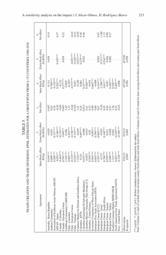
5.6. RTAs trade creation or trade diversion

Following Ghosh and Yamarik, (2004) and Eicher, Henn and Papageorgiou (2012) we use two sets of dummy variables to pick up RTA trade creation and trade diversion effects. Trade diversion occurs if a trade block creates trade in detriment of more productive third countries excluded from the agreement. The first, RTAijt, in (7) implies that both trading partners are members of the same RTA, the second, DivRTAit indicates that one country, whereas exporter or importer is a member of the RTA we are estimating.

Ghosh and Yamarik, (2004) define DivRTAit as a vector of variables which measures current membership of either country i or j in a RTA and thus, cap-tures the external effects of the RTA on trade with countries outside the zone. The coefficient ϒk for DivRTAit is interpreted as a measure of lower or higher than normal trade between nations in the trading bloc, and a country outside the bloc relative to a random pair of countries.

Hence, a negative sign for ϒk indicates less trade with non-members and is interpreted as evidence of trade diversion.

In this section, we select a group of 25 interesting RTAs to evaluate whether trade diversion is actually mitigating the impact of RTAs on trade. As in Magee (2008) our estimates point to trade creation effects for ASEAN, MERCOSUR and NAFTA. The following analysis will be based on results for the TIFE specification because some trade diversion effects could not be estimated under the TVFE specification, due possibly to collinearity problems as too many fixed effects were dropped to perform estimations.

Thus, a third of the agreements trade creation effects are mitigated by trade diversion effects. In 6 cases the intra-block trade creation effect is sufficiently strong to resist trade diversion as in Australia-Korea, Colombia-Northern Triangle, the Group of 3, ECOWAS, EC-Turkey and NAFTA. For half of the sample of analysed RTAs, the extra-block effect reinforces the intra-block trade creation effects. Conversely, the trade diversion effect outstrips the trade creation intra-block effect in ASEAN-Japan and adds to intra-block negative effects in Canada-Colombia, Chile-EC, EC-Israel and Peru-United States. See Table 5.

6. Conclusion

This paper examines the effect of regional trade agreements RTAs on international bilateral trade flows. Based on the gravity model, we perform a sensitivity analysis to the effect of the RTA dummy, applying a wide range of econometric methods and model specifications. Our database consists of an unbalanced panel for 153 countries, including observations from 1980 to 2018. Particular attention is given to Poisson Pseudo Maximum Likelihood


TAB

LE

5T

RA

DE

CR

EA

TIO

N A

ND

TR

AD

E D

IVE

RSI

ON

: PPM

L E

STIM

AT

ES

FOR

A G

RO

UP

RTA

S FR

OM

A 1

53 C

OU

NT

RIE

S 19

80-2

018

Agr

eem

ent

1In

tra-

bloc

k ef

fect

RTA

ijt

2E

xtra

-blo

ck e

ffec

tD

ivR

TAit

3 N

et e

ffec

t

4In

tra-

bloc

k ef

fect

RTA

ijt

5E

xtra

-blo

ck e

ffec

tD

ivR

TAit

6N

et e

ffec

t

Aus

tral

ia -

Kor

ea R

epub

lic0.

436*

**–0

.029

0.40

70.

114

0.02

80.

14A

ndea

n C

omm

unity

0.80

9***

0.01

90,

820.

709*

**.

A

ssoc

iatio

n of

Sou

thea

st A

sian

Nat

ions

ASE

AN

0.20

0***

0.13

7***

0,36

–0.1

92**

*.

A

SEA

N -

Jap

an0.

091*

*–0

.346

***

–0,2

60.

262*

**0.

105*

**0.

37C

anad

a -

Col

ombi

a–0

.463

***

–0.1

54**

*–0

,60

–0.1

22.

C

anad

a -

Eur

opea

n U

nion

0.59

1***

0.09

2**

0.68

30.

277*

**0.

038

0.32

Car

ibbe

an C

omm

unity

CA

RIC

OM

3.34

2***

0.10

83,

450.

828*

.

Chi

le -

Col

ombi

a0.

902*

**0.

203*

**1,

17–0

.195

*.

C

hile

- E

urop

ean

Uni

on–0

.319

***

–0.1

58**

*–0

,44

–0.3

73**

*–0

.051

***

–0.4

2C

hile

- V

ietn

am0.

534*

**0.

179*

**0.

355

0.03

1–0

.245

***

–0.2

1C

omm

on M

arke

t for

Eas

tern

and

Sou

ther

n A

fric

a 1.

234*

**–0

.019

1,21

–0.2

45–0

.671

***

–0.9

2C

olom

bia

- E

FTA

0.15

30.

097*

**0,

240.

084

0.27

5***

0.36

Col

ombi

a-(G

uate

mal

a-E

l Sal

vado

r-H

ondu

ras)

0.43

3***

–0.0

080.

813

0.43

7***

0.02

20.

46C

olom

bia-

Mex

ico-

Ven

ezue

la (

The

Gro

up o

f 3)

0.65

5*–0

.013

0,41

0.56

0***

.

Col

ombi

a -

Uni

ted

Est

ates

0.29

4***

0.05

0,32

–0.0

31.

E

cono

mic

Com

mun

ity o

f Wes

t Afr

ican

Sta

tes

0.96

3***

–0.0

93**

0,88

0.66

2***

.

Eur

opea

n Fr

ee T

rade

Ass

ocia

tion

EFT

A0.

665*

**0.

196*

**0,

86–0

.009

.

Eur

opea

n U

nion

EU

(27)

0.59

1***

0.08

4***

0,67

0.41

4***

0.05

50.

47E

urop

ean

Uni

on -

Isr

ael

–0.1

27–0

.055

–0,2

0–1

.288

***

–0.5

11**

*–1

.80

Eur

opea

n U

nion

- S

outh

Afr

ica

0.78

6***

0.14

0***

0,93

0.61

1**

0.51

6***

1.13

Eur

opea

n U

nion

- T

unis

ia0.

939*

**0.

012

0,94

0.05

10.

026

0.08

Eur

opea

n U

nion

- T

urke

y0.

490*

**–0

.002

0,51

0.16

6***

0.00

20.

17So

uthe

rn C

omm

on M

arke

t ME

RC

OSU

R1.

311*

**0.

044

1,36

0.55

6***

.

Nor

th A

mer

ican

Fre

e T

rade

Agr

eem

ent N

AFT

A0.

463*

**–0

.220

***

0,25

0.40

5***

.

Peru

- U

nite

d St

ates

–0.3

28**

*–0

.106

***

–0,4

30.

068

.

Obs

erva

tions

6741

3367

4133

45

7250

4572

50

R-s

quar

ed0.

899

0.89

9

0.95

80.

958

***

p<0.

01, *

* p<

0.05

, * p

<0.

1. R

obus

t sta

ndar

d er

rors

. Sou

rce:

Ela

bora

ted

by th

e au

thor

.N

ote:

Col

umns

(1)

and

(2)

incl

ude

time-

inva

rian

t cou

ntry

fix

ed e

ffec

ts a

nd ti

me

fixe

d ef

fect

s. C

olum

ns (

4) a

nd (

5) s

tand

for

tim

e-va

ryin

g fi

xed

effe

cts

and

coun

try-

pair

fix

ed e

ffec

ts


(PPML), which is the method that, when applied with fixed effects, best seems to contend with heteroscedasticity problems and bias from a high proportion of trade flows registered as zero.

A strong positive impact for RTA is consistently found on most specifi-cations. Once multilateral resistance and other unobserved variable bias are controlled by the introduction of time-varying country fixed effects in a PPML regression, we find that RTAs increase bilateral trade flows by 51.3%, with respect to those trade flows with no agreements. When country-pair fixed ef-fects are added to the previous specification, the RTA effect is reduced to 4.7%, still economically significant, as it confirms that efforts to close international trade deals are fruitful.

RTA cumulative effects are found using OLS, but its significance disap-pears with the PPML method. Instrumental variable methods were also tested. Using the third and the fourth lags of RTAs as instruments for RTA, as well as, employing the Hausman and Taylor estimator that introduces instrumental variables to deal with endogeneity, gives sizable and significant results.

We found considerable variations in the estimates of RTAs at the disag-gregated level. While most of these successfully increase trade, others seem to destroy it, or are non-significant. When only time-invariant fixed effects and time fixed effects were included, 71.5% of RTA were positive and significant; this number slid to 50.4% for the time-varying and country-pair fixed effects specification. Robustness checks for individual RTAs based on the comparison of the PPML time-invariant fixed effects specification and the time-varying and country-pair fixed effects specification show that 38.2% of RTAs are positive and significant in both specifications.

The wide range of individual RTA estimates [-1.139; 3.266] could be ex-plained by the fact that RTAs are heterogeneous in scope and depth. Another hypothesis points to lack of enforceability, meaning that a number of RTAs are not completely implemented in practice and remain only as a written statement, a line of research worth exploring.

Trade diversion effects were computed for a sample of RTAs. At large, trade creation effects tend to be stronger than trade diversion effects or even be reinforced by an open trade block expansion effect. Nevertheless, the po-tentiality of RTA to improve well-being must not be given for granted, as in certain cases trade diversion is found to outstrip trade creation effects.


References

Afesorgbor, S. K. (2017). “Revisiting the effect of regional integration on African trade: evidence from meta-analysis and gravity model”, Journal of International Trade and Economic Development, 26 (2): 133-153.

Ahcar, J., and Siroën, J. M. (2017). “Deep Integration: Considering the Heterogeneity of Free Trade Agreements”, Journal of Economic Integration, 32 (3): 615-659.

Anderson, J. E. (1979). “A Theoretical Foundation for the Gravity Equation”, American Economic Review, 69 (1): 106-116.

Anderson, J. E. and Van Wincoop, E. (2003). “Gravity with Gravitas: A Solution to the Border Puzzle”, The American Economic Review, 93 (1): 170-192.

Antonucci, D. and Manzocchi, S. (2006). “Does Turkey have a special trade relation with the EU?”, Economic Systems 30 (2): 157-169.

Arellano M. and Bond S. (1991). “Some Tests of Specification for Panel Data”, Review of Economic Studies, 58 (2): 277-297.

Baier S. and Bergstrand J. (2007). “Do free trade agreements actually increase members’ international trade?”, Journal of International Economics, 71 (1): 72-95.

Baier, S., Bergstrand, J. and Clance, M. (2018). “Heterogeneous effects of economic integration agreements”, Journal of Development Economics, 135: 587-608.

Baier, S., Yotov. Y. and Zylkinc, T. (2019). “On the widely differing effects of free trade agreements: Lessons from twenty years of trade integration”, Journal of International Economics. 116: 206-226.

Baldwin, R. and Jaimovich, D. (2012). “Are free trade agreements contagious?”, Journal of International Economics, 88 (1): 1-16.

Baldwin, R. and Taglioni, D. (2006). “Gravity for dummies and dummies for gravity equation”, NBER Working Paper Nº 12516.

Bas, M. and Ledezma, I. (2010). “Trade integration and within-plant productiv-ity evolution in Chile”, Review of World Economics, 146 (1): 113-146.

Bussière, M. and Schnatz, B. (2009). “Evaluating China’s Integration in World Trade with a Gravity Model Based Benchmark”, Open Economies Review, 20 (1): 85-111.

Breusch, T. and Pagan, A. (1980). “The Lagrange multiplier test and its appli-cations to model specification in econometrics”, Review of Economic Studies, 47 (1): 239-253.

Caporale, G. M., Rault, C., Sova, R., and Sova, A. (2012). “European free trade agreements and trade balance: Evidence from four new European Union members”, Journal of International Trade and Economic Development, 21 (6): 839-863. https://doi.org/10.1080/09638199.2011.555562.

Correia, S., Guimarães, P., and Zylkin, T. (2019). “PPMLHDFE: Fast pois-son estimation with high-dimensional fixed effects”, arXiv preprint arXiv:1903.01690.


De Benedictis, L. and Taglioni, D. (2011). “The gravity model in international trade”, In The Trade Impact of European Union Preferential Policies (pp. 55-89). Springer Berlin Heidelberg.

De Sousa, J. (2012). “The currency union effect on trade is decreasing over time”, Economics Letters 117 (3): 917-920.

Didia, D., Nica, M., and Yu, G. (2015). “The gravity model, African Growth and Opportunity Act (AGOA) and US trade relations with sub-Saharan Africa”, Journal of International Trade and Economic Development, 24 (8), 1130-1151. https://doi.org/10.1080/09638199.2014.1000942.

Dür, A., Baccini, L., and Elsig, M. (2014). “The design of international trade agreements: Introducing a new dataset”, The Review of International Organizations, 9 (3): 353-375.

Egger, P. and Nigai, S. (2015). “Effects of deep versus shallow trade agreements in general equilibrium”, In Trade Cooperation: The Purpose, Design and Effects of Preferential Trade Agreements (pp. 374-391). Cambridge University Press: UK.

Eicher, T. and Henn, C. (2011). “In search of WTO trade effects: Preferential trade agreements promote trade strongly, but unevenly”, Journal of International Economics, 83 (2): 137-153.

Eicher, T., Henn, C. and Papageorgiou, C. (2012). “Trade creation and diversion revisited: Accounting for model uncertainty and natural trading partner effects”, Journal of Applied Economics, 27 (2): 296- 321.

Fally, T. (2015). “Structural gravity and fixed effects”, Journal of International Economics, 97 (1): 76-85.

Ghosh, S. and Yamarik, S. (2004) “Are regional trading arrangements trade creat-ing? An application of extreme bounds analysis”, Journal of International Economics, 63 (2):369-395.

Greene, W. (2011). “Econometric Analysis”, Harlow: Pearson Education.Hayakawa, K. and Kimura, F. (2015). “How Much Do Free Trade Agreements

Reduce Impediments to Trade?”, Open Economies Review, 26 (4): 711-729.Head, K. and Mayer, T. (2014). “Gravity Equations: Workhorse, Toolkit, and

Cookbook”. Chapter 3 in Gopinath G, Helpman E, Rogoff K (eds). Handbook of International Economics, (4): 131-195.

Head K., Mayer, T. and Ries, J. (2010). “The Erosion of colonial linkages after Independence”, Journal of International Economics, 81 (1): 1-14.

Halpern, L., Koren, M. and Szeidl, A. (2015). “Imported inputs and Productivity”, American Economic Review, 105 (12): 3660-3703.

Hsiao, Ch. (2003). “Analysis of Panel Data”, Cambridge University Press.Kahouli, B. and Maktouf, S. (2015). “Trade creation and diversion effects in the

Mediterranean area: Econometric analysis by gravity model”, Journal of International Trade and Economic Development, 24 (1): 76-104.

Kim, MH. (2011). “Do We Really Know That the WTO Increases Trade? Revisited”, Global Economy Journal, 11 (2): doi:10.2202/1524-5861.1728.

Kohl, T. (2014). “Do we really know that trade agreements increase trade?” Review of World Economics, 150 (3): 443-469.


Kohl, T., Brakman, S., and Garretsen, H. (2016). “Do trade agreements stimulate international trade differently? Evidence from 296 trade agreements”, The World Economy, 39 (1): 97-131.

Larch, M., Wanner, J., Yotov, Y.V. and Zylkin, T. (2019), Currency Unions and Trade: A PPML Re-assessment with High-dimensional Fixed Effects. Oxf Bull Econ Stat, 81: 487-510. doi:10.1111/obes.12283

Magee, C. (2008). “New measures of trade creation and trade diversion”, Journal of International Economics, 75 (2): 349-362.

Martin-Mayoral, F., Morán Carofilis, G. and Cajas Guijarro, J. (2016). “The effects of integration agreements in Western Hemisphere trade, 1970-2014”, Journal of International Trade and Economic Development, 25 (5): 724-756.

Martín-Montaner, J., Requena, F. and Serrano, G. (2014). “International trade and migrant networks: Is It really about qualifications?” Estudios de Economía, 41 (2): 251-260.

Martínez-Zarzoso, I. (2013). “The log of gravity revisited”, Applied Economics, 45 (3): 311-327.

Martínez-Zarzoso, I., Nowak-Lehmann, F., and Horsewood, N. (2009). “Are regional trading agreements beneficial? Static and dynamic panel gravity models”, North American Journal of Economics and Finance, 20: 46-65.

Melitz, J. and Toubal, F. (2014). “Native language, spoken language, translation and trade”, Journal of International Economics, 93 (2): 351-363.

Mitze, T. (2010). “Estimating Gravity Model of International Trade with Correlated Time-Fixed Regressors: To IV or not to IV?”, MPRA Paper Nº 23540.

Montenegro, C. E., Pereira, M., and Soloaga, I. (2011). “El efecto de China en el comercio internacional de América Latina”, Estudios de Economia, 38 (2): 341-368. https://doi.org/10.4067/s0718-52862011000200001.

Rose, A. (2005). “Which international institution promote international trade?”, Review of International Economics, 13 (4): 682-698.

Sachs, J., Warner, A., Aslund, A. and Fischer, S. (1995). “Economic Reform and the Process of Global Integration”, Brookings Papers on Economic Activity, (1): 1-118.

Santos Silva, J. and Tenreyro, S. (2006). “The log of gravity”, Review of Economics and Statistics, 88 (4): 641-658.

Santos Silva, J. and Tenreyro, S. (2011). “Further simulation evidence on the performance of the Poisson pseudo-maximum likelihood estimator”, Econ Lett, 112 (2): 220-222.

Subramanian, A. and Wei, S. (2007). “The WTO promotes trade, strongly but unevenly”, Journal of International Economics, 72 (1): 151-175.

Swamy, P., Tavlas , G. and Hall, S. (2015). “On the interpretation of instrumental variables in the presence of specification errors”, Econometrics, 3 (1): 55-64.

Trefler, D. (1993). “Trade liberalization and the theory of endogenous protec-tion: an econometric study of U.S. import policy”, J Polit Econ, 101 (1): 138-160.


Wacziarg, R. and Welch, K. (2008). “Trade Liberalization and Growth: New Evidence”, World Bank Econ Rev, 22 (2): 187-231.

Wooldridge, J. (2012). “Introductory econometrics: A modern approach”, Cengage Learning.


APPENDIX

List of countries included in the gravity model database

Albania, Algeria, Angola, Argentina, Australia, Austria, Azerbaijan, Bahrain, Bangladesh, Barbados, Belarus, Belgium, Belize, Benin, Bermuda, Bolivia, Brazil, Brunei, Bulgaria, Burkina Faso, Burundi, Cambodia, Cameroon, Canada, Cape Verde, Central, African Republic, Chad, Chile, China, Colombia, Congo Democratic, Congo Republic, Costa Rica, Ivory Coast, Croatia, Cuba, Cyprus, Czech Republic, Denmark, Djibouti, Dominican Republic, Ecuador, Egypt, El Salvador, Equatorial, Guinea, Estonia, Ethiopia, Fiji, Finland, France, Gabon, Gambia, Georgia, Germany, Ghana, Greece, Grenada, Guatemala, Guinea, Guinea-Bissau, Guyana, Haiti, Honduras, Hong Kong, Hungary, Iceland, India, Indonesia, Iran, Iraq, Ireland, Israel, Italy, Jamaica, Japan, Jordan, Kazakhstan, Kenya, South Korea, Kuwait, Kyrgyzstan, Latvia, Lebanon, Liberia, Libya, Lithuania, Luxembourg, Madagascar, Malawi, Malaysia, Mali, Malta, Mauritania, Mauritius, Mexico, Moldova, Mongolia, Morocco, Mozambique, Nepal, Netherlands, New Zealand, Nicaragua, Niger, Nigeria, Norway, Oman, Pakistan, Panama, Papua New Guinea, Paraguay, Peru, Philippines, Poland, Portugal, Qatar, Romania, Russia, Rwanda, Samoa, Saudi Arabia, Senegal, Sierra Leone, Singapore, Slovakia, Slovenia, South Africa, Spain, Sri Lanka, Sweden, Switzerland, Syria, Tajikistan, Tanzania, Thailand, Togo, Tonga, Trinidad and Tobago, Tunisia, Turkey, Turkmenistan, Uganda, Ukraine, United Arab Emirates, United Kingdom, United States, Uruguay, Uzbekistan, Venezuela, Vietnam, Yemen, Zambia, Zimbabwe.

A sensitivity analysis on the impact of regional trade ...

Documents

Transcript of A sensitivity analysis on the impact of regional trade ...