Trade creation and trade diversion of regional trade ......Trade Creation and Trade Diversion of...
44
Trade creation and trade diversion of regional trade agreements revisited: A constrained panel pseudo-maximum likelihood approach Michael Pfaermayr Working Papers in Economics and Statistics - University of Innsbruck https://www.uibk.ac.at/eeecon/
Transcript of Trade creation and trade diversion of regional trade ......Trade Creation and Trade Diversion of...

Trade creation and trade diversion of regionaltrade agreements revisited: A constrainedpanel pseudo-maximum likelihood approach
Michael Pfaffermayr
Working Papers in Economics and Statistics
2018-10
University of Innsbruckhttps://www.uibk.ac.at/eeecon/

University of InnsbruckWorking Papers in Economics and Statistics
The series is jointly edited and published by
- Department of Banking and Finance
- Department of Economics
- Department of Public Finance
- Department of Statistics
Contact address of the editor:research platform “Empirical and Experimental Economics”University of InnsbruckUniversitaetsstrasse 15A-6020 InnsbruckAustriaTel: + 43 512 507 71022Fax: + 43 512 507 2970E-mail: [email protected]
The most recent version of all working papers can be downloaded athttps://www.uibk.ac.at/eeecon/wopec/
For a list of recent papers see the backpages of this paper.
Trade Creation and Trade Diversion of RegionalTrade Agreements Revisited: A ConstrainedPanel Pseudo-Maximum Likelihood Approach
Michael Pfaffermayr∗
July 1, 2018
Abstract
For the estimation of structural gravity models using PPML with country-pair, exporter-time and importer-time effects it proves useful to exploit theequilibrium restrictions imposed by the system of multilateral resistances.This yields an iterative projection based PPML estimator that is unaffectedby the incidental parameters problem. Further, in this setting it is straightforward to establish the asymptotic distribution of the structural parame-ters and that of counterfactual predictions. The present contribution appliesthe constrained panel PPML estimator to reconsider the trade creation andtrade diversion effects of regional trade agreements. Results show significanttrade creation effects of RTAs ranging in between 8.7 and 21.7 percent in2012, but also point to substantial trade diversion in the range of -14.4 and-5.8 percent. These counterfactual predictions account for adjustment inmultilateral trade resistances. The quite large confidence intervals of coun-terfactual predictions seem to be an overlooked issue in the literature.
Keywords: Constrained Panel Poisson Pseudo Maximum Likelihood Esti-mation; International Trade; Gravity Equation; Structural EstimationJEL: F10, F15, C13, C50
∗Department of Economic Theory, -Policy and -History University of Innsbruck, Universi-taetsstr. 15, A-6020 Innsbruck, Austria and Austrian Institute of Economic Research, E-mail:[email protected].
1 Introduction
The large number of existing regional trade agreements (RTAs) has induced whatis called a spaghetti bowl of preferential trade relationships. A myriad of papersassesses their effects on bilateral trade and welfare empirically, mainly focusing onthe trade creation effects of RTAs. In contrast, evidence on the trade diversioneffects of RTAs seems to be more scarce. The measurement of the trade creatingimpact of RTAs is typically based on gravity models of bilateral trade and RTAindicators. Identifying trade diversion effects is less straight forward. Many impor-tant contributions use a reduced form that measures trade diversion effects by adummy variable that picks out trade flows between any two countries that do notshare a RTA, but either the exporter country or the importer country (or both)are a member of one or more RTAs with other countries.1 Strictly speaking, inthis design trade diversion is modelled as if the conclusion of a RTA between anytwo countries increases trade barriers toward third non-member countries.
Economic theory predicts an adjustment of terms of trade and, therefore, mul-tilateral trade resistances, as a response to the formation of RTAs. Actually, tradediversion is a consequence of the general equilibrium effects on goods prices inducedby RTAs, but not necessarily of new trade barriers established between non-RTAmembers vis-a-vis RTA-members as a response. Contributions by, e.g., Caliendoand Parro (2015), Clausing (2001), Felbermayr et al. (2015) and Trefler (2004)consider specific trade agreements and favour a structural (general equilibrium)approach to estimate the trade creating and trade diverting effects of RTAs as wellas the implied welfare effects. In a similar vein, Bergstrand et al. (2015) estimatethe welfare effects of RTAs in a general structural gravity model in the spirit ofAnderson and van Wincoop (2003). These models fully account for the changes interms of trade via changes in the estimated multilateral resistances.
This paper reconsiders trade creation and trade diversion effects of RTAs ar-guing that in a structural gravity model the impact of trade barriers on bilateraltrade is best identified if it is modelled as a reduction in border effects. Theavailable contributions mostly include domestic trade flows, but do not interactborder dummies with the indicators of barriers to international trade. Moreover,the structural gravity model is estimated by constrained panel PPML, extend-ing the constrained PPML estimator for cross-sections introduced in Pfaffermayr(2017) to a panel setting. The constrained conditional pseudo-maximum likeli-hood approach exploits the general equilibrium restrictions imposed by the systemof trade resistances for estimation and concentrates out bilateral fixed effects. Inparticular, it is demonstrated that concentrating out country-pair fixed effects is
1See, e.g., Dai, Yotov and Zylkin (2014), Magee (2008 and 2016) and Sorgho (2016), just tomention a few important contributions. Freund and Ornelas (2010) provide a comprehensiveoverview.
equivalent to imposing further restrictions on the cross-section based constrainedPPML estimator. Hence, the available econometric results for this estimator areapplicable in a panel setting as well. More importantly, constrained panel PPMLestimation is unaffected by the incidental parameter problem in the country-pair,exporter-time and importer-time dimension arising in high-dimensional non-linearfixed effects models. The delta method allows to derive reliable confidence inter-vals for counterfactual predictions of the impact of RTAs. This approach might beseen as an alternative to bootstrapping approaches.
The empirical investigation of the impact of RTAs on trade and welfare isbased on a panel of trade flows for 65 countries observed from 1994-2012. Theestimation results indicate that border effects have substantially declined in thelast two decades. In line with the literature RTAs induce positive and quantita-tively important trade creation effects. But despite their increasing number andthe phasing in effects the impact of RTAs trade creation effects increased onlymoderately over time. On the other hand, RTAs also produced pronounced tradediversion effects. The establishment of RTAs improved welfare, especially of thosecountries with many RTAs in force, while for those with just a few RTAs in forcethe welfare gains turned out insignificant. Freezing all trade costs counterfactuallyat the level of 1992 reveals the importance of RTAs relative to non-policy relatedchanges in trade barriers. A counterfactual scenario where all international tradeflows are covered by a RTA indicates potential of welfare gains of further multilat-eral trade liberalization efforts. This scenario would induce a substantial increasein trade flows not covered by RTAs and sizeable welfare gains of countries hold-ing few RTAs. Since parameter estimation induces uncertainty to counterfactualpredictions, the involved confidence intervals are relatively large, however.
2 The Structural Panel Gravity Model
For a cross-section of C countries observed over T periods bilateral trade flows areassumed to be generated by a generic gravity model as
sijt =XijtYt,W
= Yt,W t1−σijt κitΠ
σ−1it P σ−1
jt θjteµijηijt := ez
′ijtα+βit(α,µ)+γjt(α,µ)+µijηijt. (1)
Bilateral trade flows from country i to j in period t Xijt are normalized by world
expenditures so that∑C
i=1
∑Cj=1 sijt = 1 (see Allen, Arkolakis and Takahashi,
2017). This normalization also implies that there is no constant in the model andwithout further structural assumptions on the DGP the value of world productiondenoted by Yt,W remains unspecified. Time varying trade frictions are modelled
as t1−σijt = ez′ijtα, while country-pair fixed effects µij capture time invariant unob-
served barriers to trade. κit denotes the share of country i in the value of world
2
production, while θjt refers to country j’s expenditure share in world income. Thusthe gravity model allows for trade imbalances at the country level. The countries’production and expenditure figures are assumed to be exogenously given, so Yt,Wis given as well and for asymptotic analysis it is assumed to grow at the rate ofthe number of country pairs C2. The disturbances ηij have E[ηijt|zijt] = 1 and canbe heteroskedastic or clustered in the country pair dimension, or even clusteredin exporter-time, importer-time and country-pair dimension (Egger and Tarlea,2015).
Multilateral trade resistances enter the model in normalized form as eβit(α,µ) =κitΠit(α, µ)σ−1 and eγjt(α,µ) = θjtPjt(α, µ)σ−1 and depend on the parameter vectorα referring to trade barriers, the country-pair specific fixed effects µij, the aggregatesales and expenditure shares of the countries and on the number of countries inthe sample. Thus the DGP changes with the number of countries and sijt formsa triangular array.2 For i, j = 1, ..., C and period t the system of trade resistancescan be compactly written as
κit =C∑j=1
ez′ijtα+βit(α,µ)+γjt(α,µ)+µij (2)
θjt =C∑i=1
ez′ijtα+βit(α,µ)+γjt(α,µ)+µij . (3)
In the absence of any trade barriers (i.e., α = 0, µij = 0) one can set Πit(0, 0) = ctand Pjt(0, 0) = 1/ct, where ct is a time-specific constant so that eβit(0,0) = ctκit andeγjt(0,0) = θjt/ct. Since the solutions of the system of trade resistances are uniqueup to a constant trade, the multilateral resistances have to be normalized andit is assumed that βCt = 0, t = 1, ..., T . Furthermore, the country pair fixedeffects need to be normalized as well to obtain a full rank dummy design matrix.Actually, in this three-way model only (C − 1)2 country-pair effects are identifiedin the presence of exporter-time and importer-time effects. Thus, without loss ofgenerality one may set µii = 0 and µCj = 0, i, j = 1, ..., C.
For estimation the structural gravity model can be reformulated in an abbre-viated notation with additive disturbances
sijt = mijt(ϑ) + εijt, εijt = mijt(ϑ) (ηijt − 1) , (4)
where mijt(ϑ) = ez′ijtα+βit(α,µ)+γjt(α,µ)+µij , ϑ = [φ(α, µ)′, µ′]′, φ = [α′, β′(α, µ),
γ′(α, µ)]′. Santos Silva and Windemeijer (1997) show that in a PPML or a methodof moments framework with exogenous explanatory variables the multiplicative and
2To avoid clutter the index C that indicates triangular arrays is skipped throughout.
3
additive model are observationally equivalent and lead to the same estimators,since they are based on a the same conditional mean assumptions. Under IV-estimation, this equivalence breaks down, however.
3 The Constrained Panel PPML Estimator
The proposed constrained panel PPML estimator exploits the restrictions im-posed by the system of multilateral resistances and maximizes the conditionalPoisson likelihood under the constraint θφ − D′φm(ϑ) = 0, where θφ is definedas (κ11, ..., κC−1,T , θ11, .., θCT )′. As a result the predicted bilateral trade flows ofthat model adhere to adding-up constraints and aggregate exactly to productionand expenditures for each country. This implies that the estimation procedureimplicitly predicts missing trade flows.
Following Hausman, Hall and Grilliches (1984), Palmgren (1981) and Wooldridge(1999) fixed country-pair effects can be eliminated by conditioning on
∑Tt=1 vijtsijt
(or concentrating out µij). As shown in the Appendix A.1 maximizing the condi-tional Poisson likelihood under the constraint D′φm(ϑ)− θφ is equivalent to apply-ing the constrained PPML estimator for cross-sections as analyzed in Pfaffermayr(2017) with the additional restriction
∑Tt=1 vijtmijt(ϑ) =
∑Tt=1 vijtsijt := θµ,ij.
Thereby, the country-pair specific trade flow averages are collected in θµ, where θµis a (C − 1)2× 1 vector with typical element
∑Tt=1 vijtsijt.
3 For estimation the ele-ments of θµ are held fixed and treated as non-stochastic. Specifically, in AppendixA.1 it is shown that this approach leads to the same score, and thus the sameestimates, as that obtained by maximizing the constrained conditional likelihoodof the panel.
The introduction of the restriction θµ −D′µV m(ϑ) = 0 is for convenience as itallows to apply Proposition 2 in Pfaffermayr (2017) to establish the asymptoticdistribution of structural parameters α. Therefore, the constrained panel PPMLestimator of α is not affected by the incidental parameters, since at a given estimateα, the parameter estimates of all dummies, including the country-pair fixed effects,are uniquely determined by the imposed restrictions. Maximizing the constrainedlikelihood is equivalent to maximizing the conditional likelihood or, equivalently,one that concentrates out µij and imposing the restrictions implied by the systemof trade resistances only.
The score: The K + T (2C − 1) + C(C − 1) explanatory variables (including alldummies) are collected in W = [Z,D] and D = [Dφ, V Dµ] where Dφ includes all
3Principally, θµ may include out of sample information to form the sums of a country-pair’snormalized trade flows over time (see Blundell, Griffith and Windmeijer, 2002 and Anderson andYotov, 2016).
4
dummies capturing multilateral resistances and Dµ the dummies for the countrypair-fixed effects. Since the panel is possibly unbalanced, the diagonal selectionmatrix V with elements vijt indicates whether a trade flow is observed (vijt = 1)or missing (νijt = 0). Conditional on Z and D missingness has to occur at randomfor constrained panel PPML estimators to be consistent.
Defining θ = (θ′µ, θ′φ)′, the score of constrained panel PPML can be compactly
written as
∂ lnLC(ϑ|V,W, θ)∂ϑ
= W ′V (s−m(ϑ)) +W ′M(ϑ)Dλ (5)
∂ lnLC(ϑ|V,W, θ)∂λ
= θ −D′m(ϑ),
where λ is a (C−1)2+T (2C−1)×1 vector of Lagrange multipliers. Appendix A.1demonstrates that solving (5) yields the same solutions as those of the constrainedconditional Poisson likelihood given by
0 = W ′φQµ(ϑ)V s−W ′
φQµ(ϑ)M(ϑ)Dφλφ (6)
0 = θφ −D′φm(ϑ)
Thereby Qµ(ϑ) =(ITC2 −M(ϑ)V Dµ
(D′µVM(ϑ)Dµ
)−1D′µ
)is a projection ma-
trix with D′µQµ(ϑ) = 0, which is is not symmetric, however.
Iterative estimation procedure: For estimation one may apply an iterative,constrained, projection based estimation procedure similar to that put forward inFalocci, Paniccia and Stanghellini (2009). For cross-section gravity models it isdescribed in detail in Pfaffermayr (2017) and for panels in Appendix A.2. Usingnested iterations in a partial Gauss-Seidel algorithm (Guimaraes and Portugal,2010 and Smyth, 1996) avoids the inversion of large matrices in the presence thecountry-pair dummies.
In order to describe the proposed iterative estimation procedure it is useful todefine the following vectors and matrices. Thereby, the index r indicates the r-thiteration step and to simplify notation arguments are skipped.
mijt,φ,r = ez′ijtαr+βit(αr,µr)+γjt(αr,µr) (7)
πij,r = eµij,r
Mr = diag(mijt,φ,rπij,r)
Qµ,r = ITC2 − MrV Dµ
(D′µV MrDµ
)−1D′µ
5
Gr = W ′φV Qµ,rWφ, Wφ = [Z,Dφ]
Fr = D′φMrQµ,rWφ
where Gr is assumed to be non-singular. Given iteration r, iteration step r + 1proceeds with the following calculations:
1. φr+1 = φr +
(G−1r − G−1r F ′r
(FrG
−1r F ′r
)−1FrG
−1r
)W ′φV (s− mr)
+G−1r F ′r
(FrG
−1r F ′r
)−1 (θφ −D′φmr
)2. πr+1 = (D′µVM(φC,r+1, πr)Dµ)−1Mπ,rθµ
3. Calculate mijt,r+1 = mijt,φ,r+1πij,r+1, Qµ,r+1, Gr+1, Fr+1 and iterate until con-vergence.
Starting values may come from unconstrained panel PPML estimators. Since un-constrained PPML is often based on different dummy designs and normalizations,one can use the estimated slope values α1 derived from panel PPML with exporter-time and importer-time dummies, but start with the solution of the system of traderesistances at α = 0, i.e., φ1 = (α′1, θ
′φ)′ and calculate, π1 as in step 2. This itera-
tive estimation procedure of constrained panel PPML model is very similar to thatfor the cross-section estimates. The only difference is the usage of the projectionmatrix Qµ,r used in the estimation of φr+1 in step 1 and the intermediate step 2to estimate πr+1. With this step one avoids the inversion of large matrices arisingfrom the country-pair dummies in step 1.
Asymptotic distribution of α: Since the first order conditions of the con-strained panel PPML estimator (5) are identical to those of cross-sectional con-strained PPML, Proposition 2 in Pfaffermayr (2017) applies to establish the limit
distribution of CT12 (α − α0). In fact, this proposition states that under a set of
regularity conditions and independent, but heteroskedastic disturbances the con-strained panel PPML estimator α is consistent and asymptotically normal with
CT12 (α− α0)
d→ N(0, B−10 A0ΩεA
′0B−10
), (8)
where Ωε = diag(σ2ij), A0ΩεA
′0 = p limC→∞
1TC2A(α∗)εε′A(α∗)′, B0 = p limC→∞B(α∗),
with α∗ lying in between those of α and α0, element by element and
A(α) = TC2Z ′(ITC2 −M(α)D′(F (α)G(α)−1F (α)′
)−1F (α)G(α)−1W ′)V
B(α) = Z ′V[M(α)−M(α)D(D′M(α)D)−1D′M(α)
]Z, (9)
6
where M(α) = diag(mijt(α)), G(α) = W ′VM(α)W and F (α) = D′M(α)W ,respectively. Since α is consistent, it can be plugged in for α0 using B(α) and1
TC2A(α)diag(εε′)A(α)′ to obtain a consistent estimates of B0 and 1TC2A0ΩεA0
′.The normalization differs from the standard approach as mijt(α) and E(ε2ij) areassumed to be o(C−2) and op(C
−4), respectively, to account for the normalizationof trade flows by world expenditures.
It can be shown that under fully observed trade flows limit distribution ofthe constrained panel PPML estimator is identical to that of a panel Poissonmodel with country-pair, exporter-time, importer-time fixed effects (see Avis andShepherd, 2013 and Fally, 2015). In a setting with trade flows missing at randomthe limit distribution is different, however. Pfaffermayr (2017) demonstrates forthe cross-section model that standard errors of α estimated by dummy PPMLare downward biased because the variance of the estimated exporter and importereffects contribute the estimated variance of the score, while the DGP assumesthat these are functionally dependent on α. This leads to oversized t-tests andto incorrect coverage rates of confidence intervals for the structural parameters, ifthey are estimated by dummy PPML.
Figueiredo, Guimaraes and Woodward (2015) propose a zig-zag Gauss-Seidelalgorithm to estimate a high dimensional three-way fixed effects model efficiently(without imposing the restrictions if the system of trade resistances). Moreover,these authors propose a clever way to estimate standard errors of the structuralparameter vector α consistently using within transformed residuals. It turns outthat their approach is identical to that proposed here, when V = 1 and trade flowsare fully observed.
Alternatively, under appropriate regularity conditions it is possible to calculateclustered standard errors following Cameron, Gelbach and Miller (2011), Eggerand Tarlea (2015) and Pfaffermayr (2017). If disturbances are correlated withincountry pairs, e.g. due to serial correlation, it is important to cluster standarderrors along this dimension. The corresponding selection matrix picks out C2
country-pair clusters and can be defined as DµD′µ. Then one can show that it
holdsA0ΩεA0 = p lim
C→∞1C2A(α∗)
(εε′ DµD
′µ
)A(α∗), (10)
where the Hadarmard element-wise product is denoted by . If disturbances areadditionally correlated across importers and exporters at each point in time, e.g.,induced by unobserved random exporter-year and importer-year specific shocks,the multi-way clustering approach of Cameron, Gelbach and Miller (2011) can beapplied. In this case, the elements of the selector matrices take the value of 1 ifany two observations with indices ij, it or jt belong to the same country-pairs,exporter-year or importing-year cluster, respectively. Using the dummy designmatrices Dxt to select the exporter-time specific and Dmt the importer-time specific
7
clusters, one obtains under this more general assumption on the disturbances andappropriate regularity conditions
A0ΩεA0 = p limC→∞
1(CT )3
A(α∗) (εε′ S)A(α∗). (11)
In line with Egger and Tarlea (2015) the selection matrix is specified as
S = DµD′µ +DxtD
′xt +DmtD
′mt (12)
−((DµD
′µ
) (DxtD
′xt)−
(DµD
′µ
) (DxtD
′xt) + (DmtD
′mt) (DxtD
′xt))
+ ITC2 .
The limiting matrix A0ΩεA0 of the estimated parameters can again be estimatedconsistently, by plugging in the estimated residuals of constrained panel PPMLestimator for disturbances ε. However the rate of convergence in this case is slower.For example, in the under three-way clustering α − α0 needs to be normalizedby (CT )
12 rather than by CT
12 to establish the limit distribution (see Cameron,
Gelbach and Miller, 2011, p. 247-248).
Comparative static predictions: The delta method allows to derive the asymp-totic distribution of counterfactual predictions for aggregates or finite subsets ofbilateral trade flows. Thereby, the selection matrix R picks out a finite set ofcountry pairs and aggregates them accordingly. The rank of R has to be smallerthan the number of the estimated structural parameters. Let superscript c de-note counterfactuals arising from of changes in trade barriers from Z to Zc. Thematrices without superscript refer to the baseline. Defining
Υc0 = lim
C→∞RM(α0)
−1M c(α0)[ITC2 −D (D′M c(α0)D)−1D′M c(α0)]Z
c (13)
Υ0 = limC→∞
RM(α0)−1M c(α0)[ITC2 −D (D′M(α0)D)
−1D′M(α0)]Z
one can show (see the Appendix A.4 for details) that under a set of regularityconditions it holds
CT12R(M(α)−1mc(α)−M(α0)
−1m(α0
)) (14)
d→ N(0, (Υc0 −Υ0)Vα (Υc
0 −Υ0)′),
where Vα = B−10 A0ΩεA′0B−10 . Furthermore, R
(Υc − Υ
)− R (Υc
0 −Υ0) = op(1).
The estimates of counterfactual changes and their standard errors likewise remainunaffected by the nuisance parameters µij and by the dummies for the trade resis-tance terms as these are fully determined by the set of constraints at given α andprojected out.
8
Monte Carlo simulations: A small scale Monte Carlo analysis shows that theproposed iterative estimation procedure works well in medium sized panels andallows proper inference on both the estimated parameters and the counterfactualchanges in predicted trade flows. The simulations are based on a set of 20 countriesobserved over 4 periods (1997, 2000, 2003, 2006) using the same database as theempirical analysis below. The estimated model includes a border dummy and logdistance both interacted with time dummies for 2000, 2003 and 2006 as well as aRTA dummy.
The true slope parameters and the country-pair fixed effects are taken from ainitial panel PPML regression with fixed country-pair, exporter-time and importer-time effects. The true trade resistance parameters are then derived as solutions ofthe corresponding system of trade resistance equations.
In principle, under unrestricted disturbances the gravity model may predictnegative trade flows. Thus the disturbances are generated from independent ran-dom variables that are distributed as truncated normal on [−0.0396, 0.0396]. Inline with the regularity assumptions for the asymptotic analysis, the bounds of thetruncated normal are chosen to avoid negative predicted trade flows and boundsare tighter the higher the standard deviation of the underlying non-truncated nor-mal. In a second step, the disturbances are transformed to obtain an expectedvalue of 1 and a standard deviation of either 0.01 and 0.05, respectively. Thesedisturbances enter the true model multiplicatively so that a model estimated underthe assumption of additive disturbances is heteroskedastic (see eq. 4). Under thisdata generating process one obtains t-values for the estimated slope parametersthat are comparable to those of estimated gravity models.
The model is simulated for the fully observed panel as well as for an unbalancedpanel with 50% of the observations missing in the first three periods. Thereby, itis assumed that the last wave of trade flows is fully observed to guarantee thatfixed country-pair effects can be derived from at least one country-pair observation.All Monte Carlo experiments are based on 10000 replications. Since the MonteCarlo simulations themselves add noise, the simulated coverage ratios have to becompared to their confidence intervals amounting to [0.988, 0.992], [0.946, 0.954]and [0.894, 0.906] for the 99%, 95% and 90% confidence intervals, respectively.
Table 1 reports simulated coverage ratios of the confidence intervals of one slopeparameter (the border effect in the year 1997) and of the impact of counterfactuallyeliminating country borders for those countries, whose size is below the median.With independent disturbances the coverage rates of the confidence intervals comevery close to their nominal values both in case of the estimated slope parameteras well as for the counterfactual prediction. This also holds if 50 percent of theobservations are missing. For the parameter estimate all simulated coverage rates
9
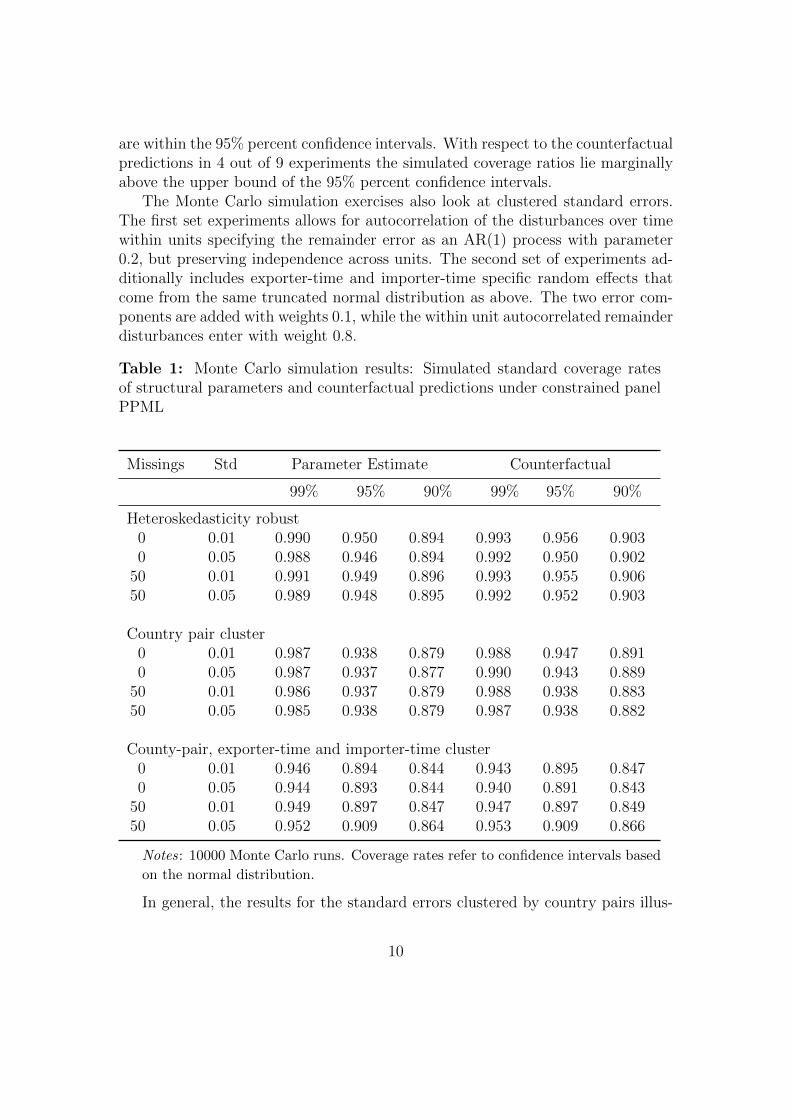
are within the 95% percent confidence intervals. With respect to the counterfactualpredictions in 4 out of 9 experiments the simulated coverage ratios lie marginallyabove the upper bound of the 95% percent confidence intervals.
The Monte Carlo simulation exercises also look at clustered standard errors.The first set experiments allows for autocorrelation of the disturbances over timewithin units specifying the remainder error as an AR(1) process with parameter0.2, but preserving independence across units. The second set of experiments ad-ditionally includes exporter-time and importer-time specific random effects thatcome from the same truncated normal distribution as above. The two error com-ponents are added with weights 0.1, while the within unit autocorrelated remainderdisturbances enter with weight 0.8.
Table 1: Monte Carlo simulation results: Simulated standard coverage ratesof structural parameters and counterfactual predictions under constrained panelPPML
Missings Std Parameter Estimate Counterfactual
99% 95% 90% 99% 95% 90%
Heteroskedasticity robust0 0.01 0.990 0.950 0.894 0.993 0.956 0.9030 0.05 0.988 0.946 0.894 0.992 0.950 0.902
50 0.01 0.991 0.949 0.896 0.993 0.955 0.90650 0.05 0.989 0.948 0.895 0.992 0.952 0.903
Country pair cluster0 0.01 0.987 0.938 0.879 0.988 0.947 0.8910 0.05 0.987 0.937 0.877 0.990 0.943 0.889
50 0.01 0.986 0.937 0.879 0.988 0.938 0.88350 0.05 0.985 0.938 0.879 0.987 0.938 0.882
County-pair, exporter-time and importer-time cluster0 0.01 0.946 0.894 0.844 0.943 0.895 0.8470 0.05 0.944 0.893 0.844 0.940 0.891 0.843
50 0.01 0.949 0.897 0.847 0.947 0.897 0.84950 0.05 0.952 0.909 0.864 0.953 0.909 0.866
Notes: 10000 Monte Carlo runs. Coverage rates refer to confidence intervals based
on the normal distribution.
In general, the results for the standard errors clustered by country pairs illus-
10
trate that the approximation of the asymptotic distribution somewhat is weaker.In case of disturbances clustered by country pairs the simulated coverage rates forthe estimated parameters are slightly below their nominal rates and marginallyoutside the confidence interval, especially at significance level of 0.1. The coveragerates referring to the counterfactuals come close to the nominal values in the fullyobserved panel. However, with 50% missings the coverage rates are somewhatlower and fall outside the 95% interval. For example, at a 5 percent significancelevel the simulated coverage rate amounts to 0.938 and at a 10% level it is foundto be 0.882, but the confidence interval is [0.894, 0.906].
In case of the three-way clustered standard errors 11, 659 out of 40, 000 MonteCarlo runs delivered negative definite estimated variance covariance matrices cast-ing some doubt on the validity of Monte Carlo results. This issue is well docu-mented in the literature and discussed in Cameron, Gelbach and Miller (2011). Ittends to occur in models with fixed effects and clustering in the same dimensions.These Monte Carlo runs have been skipped in the corresponding figures reportedin Table 1. In the valid runs the coverage rates of the confidence intervals lie belowtheir nominal values across the board by about 5 percentage points, indicating aweaker approximation by the normal and possible selection effects.
4 Empirical Evidence on Trade Creation and Trade
Diversion
The Econometric Specification of the Structural Gravity Model: Thespecification of the gravity model closely follows Bergstrand et al. (2015), Borchertand Yotov (2017) and Dai, Yotov and Zylkin (2014), who argue that the structuralgravity model identifies the cost of international trade relative to domestic tradecosts. For this reason the bilateral trade data include domestic trade flows fromcountry i into i itself. Further, in a panel setting with data exhibiting variationover time, the gravity model can be estimated with country-pair fixed effects tocontrol for unobserved time invariant determinants of barriers to trade and toguard against the endogeneity of RTA indicators as observed in cross-sections (seeBaier and Bergstrand, 2007).
The econometric specification of the structural gravity model accounts for sec-ular globalisation trends as described in Yotov (2012) and Borchert and Yotov(2017). Specifically, it includes border dummies Bij, taking the value 1 if i 6= jand 0 else, that are interacted with time dummies Tt (with exception of the firstperiod) to measure the change of border effects over time. The evolution of the bor-der effects may differ for more distant trading partners and for non-neighbouringcountries. Hence, the border-year effects are additionally interacted with ln distij
11
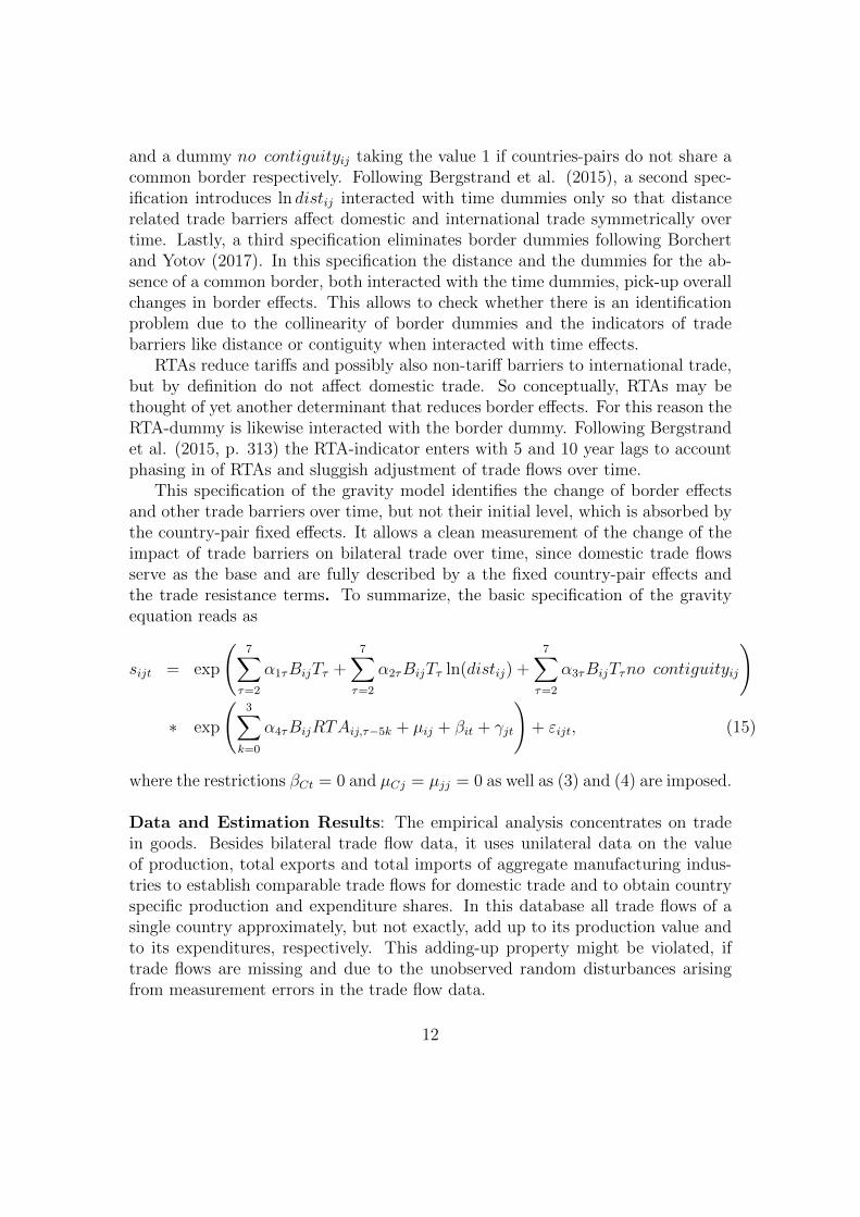
and a dummy no contiguityij taking the value 1 if countries-pairs do not share acommon border respectively. Following Bergstrand et al. (2015), a second spec-ification introduces ln distij interacted with time dummies only so that distancerelated trade barriers affect domestic and international trade symmetrically overtime. Lastly, a third specification eliminates border dummies following Borchertand Yotov (2017). In this specification the distance and the dummies for the ab-sence of a common border, both interacted with the time dummies, pick-up overallchanges in border effects. This allows to check whether there is an identificationproblem due to the collinearity of border dummies and the indicators of tradebarriers like distance or contiguity when interacted with time effects.
RTAs reduce tariffs and possibly also non-tariff barriers to international trade,but by definition do not affect domestic trade. So conceptually, RTAs may bethought of yet another determinant that reduces border effects. For this reason theRTA-dummy is likewise interacted with the border dummy. Following Bergstrandet al. (2015, p. 313) the RTA-indicator enters with 5 and 10 year lags to accountphasing in of RTAs and sluggish adjustment of trade flows over time.
This specification of the gravity model identifies the change of border effectsand other trade barriers over time, but not their initial level, which is absorbed bythe country-pair fixed effects. It allows a clean measurement of the change of theimpact of trade barriers on bilateral trade over time, since domestic trade flowsserve as the base and are fully described by a the fixed country-pair effects andthe trade resistance terms. To summarize, the basic specification of the gravityequation reads as
sijt = exp
(7∑
τ=2
α1τBijTτ +7∑
τ=2
α2τBijTτ ln(distij) +7∑
τ=2
α3τBijTτno contiguityij
)
∗ exp
(3∑
k=0
α4τBijRTAij,τ−5k + µij + βit + γjt
)+ εijt, (15)
where the restrictions βCt = 0 and µCj = µjj = 0 as well as (3) and (4) are imposed.
Data and Estimation Results: The empirical analysis concentrates on tradein goods. Besides bilateral trade flow data, it uses unilateral data on the valueof production, total exports and total imports of aggregate manufacturing indus-tries to establish comparable trade flows for domestic trade and to obtain countryspecific production and expenditure shares. In this database all trade flows of asingle country approximately, but not exactly, add up to its production value andto its expenditures, respectively. This adding-up property might be violated, iftrade flows are missing and due to the unobserved random disturbances arisingfrom measurement errors in the trade flow data.
12
Data come from several sources and are described in detail in Appendix B.Bilateral trade flow data are taken from OECD’s STAN database and Nicita andOlarreaga’s 2007 database, covering the period 1994-2012 in three-years intervals.Data on gross-production, total exports and total imports are collected from severalsources (OECD-STAN, UNIDO, CEPII and WIOD). These figures are carefullychecked to be consistent with the data on bilateral trade flows and that noneof the country specific figures is missing. Thereby, a few data points have beeninterpolated. Lastly, population weighted geographical distances and the dummyfor contiguity are taken from Mayer and Zignago (2011), while the information onRTAs is provided by Mario Larch’s Regional Trade Agreements Database describedin Egger and Larch (2008). The RTA-dummy takes the value 1 if either a customsunion or a free trade area has been established and zero otherwise.
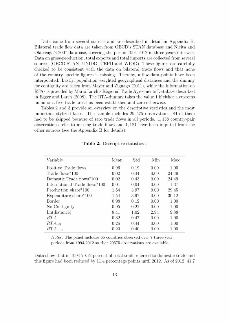
Tables 2 and 3 provide an overview on the descriptive statistics and the mostimportant stylized facts. The sample includes 29, 575 observations, 84 of themhad to be skipped because of zero trade flows in all periods. 1, 138 country-pairobservations refer to missing trade flows and 1, 184 have been imputed from theother sources (see the Appendix B for details).
Table 2: Descriptive statistics I
Variable Mean Std Min Max
Positive Trade flows 0.96 0.19 0.00 1.00Trade flows*100 0.02 0.44 0.00 24.49Domestic Trade flows*100 0.02 0.43 0.00 24.49International Trade flows*100 0.01 0.04 0.00 1.37Production share*100 1.54 3.97 0.00 29.45Expenditure share*100 1.54 3.97 0.00 30.12Border 0.98 0.12 0.00 1.00No Contiguity 0.95 0.22 0.00 1.00Ln(distance) 8.41 1.02 2.94 9.88RTA 0.32 0.47 0.00 1.00RTA−5 0.26 0.44 0.00 1.00RTA−10 0.20 0.40 0.00 1.00
Notes: The panel includes 65 countries observed over 7 three-year
periods from 1994-2012 so that 29575 observations are available.
Data show that in 1994 79.12 percent of total trade referred to domestic trade andthis figure had been reduced by 11.4 percentage points until 2012. As of 2012, 41.7
13
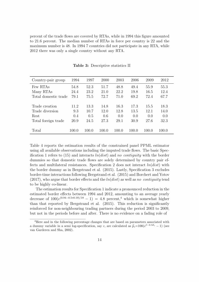
percent of the trade flows are covered by RTAs, while in 1994 this figure amountedto 21.6 percent. The median number of RTAs in force per country is 22 and themaximum number is 48. In 1994 7 countries did not participate in any RTA, while2012 there was only a single country without any RTA.
Table 3: Descriptive statistics II
Country-pair group 1994 1997 2000 2003 2006 2009 2012
Few RTAs 54.8 52.3 51.7 48.8 49.4 55.9 55.3Many RTAs 24.4 23.2 21.0 22.2 19.8 16.5 12.4Total domestic trade 79.1 75.5 72.7 71.0 69.2 72.4 67.7
Trade creation 11.2 13.3 14.8 16.3 17.3 15.5 18.3Trade diversion 9.3 10.7 12.0 12.8 13.5 12.1 14.0Rest 0.4 0.5 0.6 0.0 0.0 0.0 0.0Total foreign trade 20.9 24.5 27.3 29.1 30.9 27.6 32.3
Total 100.0 100.0 100.0 100.0 100.0 100.0 100.0
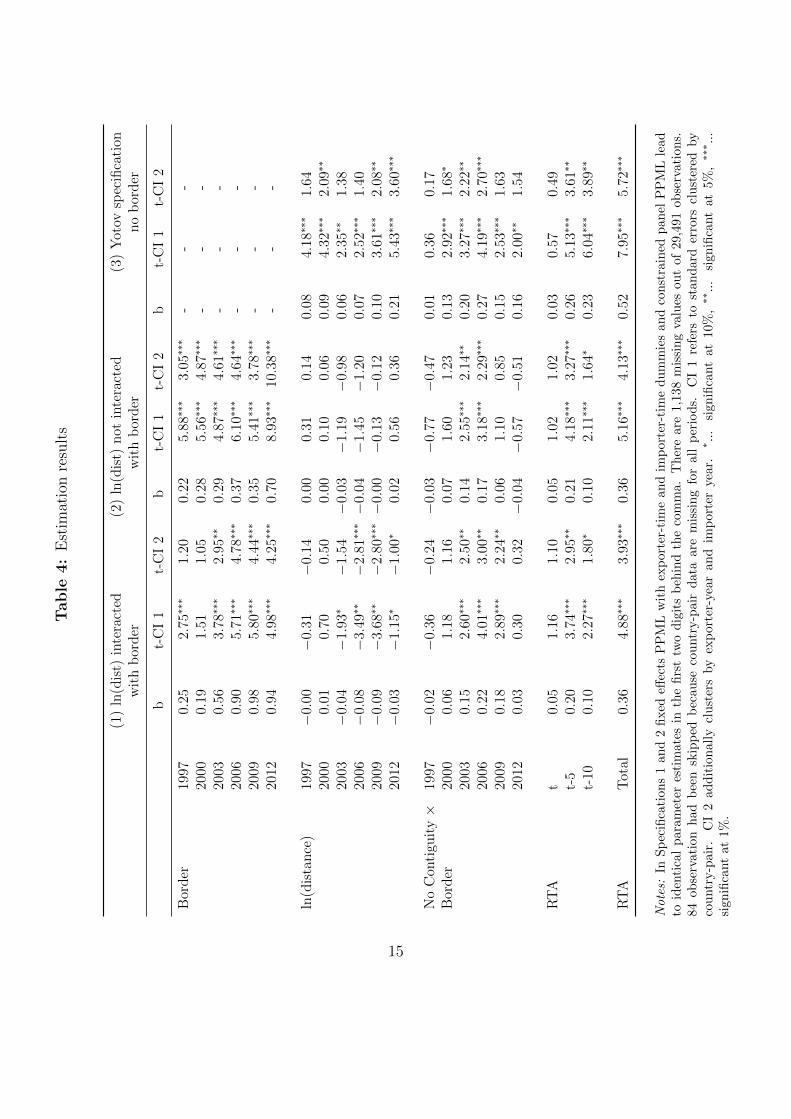
Table 4 reports the estimation results of the constrained panel PPML estimatorusing all available observations including the imputed trade flows. The basic Spec-ification 1 refers to (15) and interacts ln(dist) and no contiguity with the borderdummies so that domestic trade flows are solely determined by country pair ef-fects and multilateral resistances. Specification 2 does not interact ln(dist) withthe border dummy as in Bergstrand et al. (2015). Lastly, Specification 3 excludesborder-time interactions following Bergstrand et al. (2015) and Borchert and Yotov(2017), who argue that border effects and the ln(dist) as well as no contiguity tendto be highly co-linear.
The estimation results for Specification 1 indicate a pronounced reduction in theestimated border effects between 1994 and 2012, amounting to an average yearlydecrease of 100(e(0.94−0.5∗0.19)/18 − 1) = 4.8 percent,4 which is somewhat higherthan that reported by Bergstrand et al. (2015). This reduction is significantlyreinforced for non-neighbouring trading partners during the period 2003 to 2009,but not in the periods before and after. There is no evidence on a fading role of
4Here and in the following percentage changes that are based on parameters associated witha dummy variable in a semi log-specification, say c, are calculated as pc=100(ec−0.5σc − 1) (seevan Garderen and Sha, 2002).
14
Table
4:
Est
imat
ion
resu
lts
(1)
ln(d
ist)
inte
ract
ed(2
)ln
(dis
t)not
inte
ract
ed(3
)Y
otov
spec
ifica
tion
wit
hb
order
wit
hb
order
no
bor
der
bt-
CI
1t-
CI
2b
t-C
I1
t-C
I2
bt-
CI
1t-
CI
2
Bor
der
1997
0.25
2.75∗∗∗
1.20
0.22
5.88∗∗∗
3.05∗∗∗
--
-20
000.
191.
511.
050.
285.
56∗∗∗
4.87∗∗∗
--
-20
030.
563.
78∗∗∗
2.95∗∗
0.29
4.87∗∗∗
4.61∗∗∗
--
-20
060.
905.
71∗∗∗
4.78∗∗∗
0.37
6.10∗∗∗
4.64∗∗∗
--
-20
090.
985.
80∗∗∗
4.44∗∗∗
0.35
5.41∗∗∗
3.78∗∗∗
--
-20
120.
944.
98∗∗∗
4.25∗∗∗
0.70
8.93∗∗∗
10.3
8∗∗∗
--
-
ln(d
ista
nce
)19
97−
0.00
−0.
31−
0.14
0.00
0.31
0.14
0.08
4.18∗∗∗
1.64
2000
0.01
0.70
0.50
0.00
0.10
0.06
0.09
4.32∗∗∗
2.09∗∗
2003
−0.
04−
1.93∗
−1.
54−
0.03
−1.
19−
0.98
0.06
2.35∗∗
1.38
2006
−0.
08−
3.49∗∗
−2.
81∗∗∗−
0.04
−1.
45−
1.20
0.07
2.52∗∗∗
1.40
2009
−0.
09−
3.68∗∗
−2.
80∗∗∗−
0.00
−0.
13−
0.12
0.10
3.61∗∗∗
2.08∗∗
2012
−0.
03−
1.15∗
−1.
00∗
0.02
0.56
0.36
0.21
5.43∗∗∗
3.60∗∗∗
No
Con
tigu
ity×
1997
−0.
02−
0.36
−0.
24−
0.03
−0.
77−
0.47
0.01
0.36
0.17
Bor
der
2000
0.06
1.18
1.16
0.07
1.60
1.23
0.13
2.92∗∗∗
1.68∗
2003
0.15
2.60∗∗∗
2.50∗∗
0.14
2.55∗∗∗
2.14∗∗
0.20
3.27∗∗∗
2.22∗∗
2006
0.22
4.01∗∗∗
3.00∗∗
0.17
3.18∗∗∗
2.29∗∗∗
0.27
4.19∗∗∗
2.70∗∗∗
2009
0.18
2.89∗∗∗
2.24∗∗
0.06
1.10
0.85
0.15
2.53∗∗∗
1.63
2012
0.03
0.30
0.32
−0.
04−
0.57
−0.
510.
162.
00∗∗
1.54
RT
At
0.05
1.16
1.10
0.05
1.02
1.02
0.03
0.57
0.49
t-5
0.20
3.74∗∗∗
2.95∗∗
0.21
4.18∗∗∗
3.27∗∗∗
0.26
5.13∗∗∗
3.61∗∗
t-10
0.10
2.27∗∗∗
1.80∗
0.10
2.11∗∗∗
1.64∗
0.23
6.04∗∗∗
3.89∗∗
RT
AT
otal
0.36
4.88∗∗∗
3.93∗∗∗
0.36
5.16∗∗∗
4.13∗∗∗
0.52
7.95∗∗∗
5.72∗∗∗
Notes:
InSp
ecifi
cati
ons
1an
d2
fixed
effec
tsP
PM
Lw
ith
exp
ort
er-t
ime
and
imp
ort
er-t
ime
du
mm
ies
and
con
stra
ined
panel
PP
ML
lead
toid
enti
cal
par
amet
eres
tim
ates
inth
efirs
ttw
odig
its
beh
ind
the
com
ma.
Ther
eare
1,1
38
mis
sin
gva
lues
out
of
29,4
91
ob
serv
ati
ons.
84ob
serv
atio
nhad
bee
nsk
ipp
edb
ecau
seco
untr
y-p
air
data
are
mis
sing
for
all
per
iods.
CI
1re
fers
tost
and
ard
erro
rscl
ust
ered
by
countr
y-p
air.
CI
2ad
dit
ion
ally
clu
ster
sby
exp
orte
r-ye
ar
an
dim
port
erye
ar.
∗ ...
signifi
cant
at
10%
,∗∗
...
signifi
cant
at
5%
,∗∗
∗ ...
sign
ifica
nt
at1%
.
15
distance as a barrier to trade (i.e., for reducing border effects) once it is controlledfor border effects and no-contiguity as is also found in Bergstrand et al. (2015). Tothe contrary, border effects for more distant countries are increasing in the years2003 to 2009 all else equal. Applying the Bergstrand et al. (2015) Specification2, where distance is not interacted with border dummies reveals insignificant dis-tance related effects, while the interactions of no contiguity with border turn outsmaller, but significantly positive for 2003 and 2006.
Estimation results for Specification 3 confirm the finding of Bergstrand et al.(2015) and Borchert and Yotov (2017) and indicate a fading role of distance as abarrier to trade over time if border dummies are not included. These estimatesalso pick up the reduction in border effects in general and do not isolate the changein the impact of average distance that would be captured by border-time inter-actions. As stated by Bergstrand. et al (2015, p. 301) ”the declining effect ofinternational borders on trade and of distance on trade are two sides of the samecoin; international trade costs have likely been declining relative to intranationaltrade costs.” Thus, there seems to be an inherent identification problem in esti-mating the changing impact of distance on bilateral trade flows.
The estimated impact of RTAs on bilateral trade flows turns out very similarin the first two specifications. The estimation results point to an economicallyimportant and significant direct trade enhancing effect of RTAs with pronouncedphasing in patterns. In Specification 1, after 10 years the direct impact of RTAson bilateral trade flows accumulates to an increase of 100∗(e0.36−0.5∗0.07−1) = 38.4percent, an estimate at the lower end of those available in the literature (see Headand Mayer, 2014). The estimation results of Specification 3 imply a higher ac-cumulated impact of RTAs amounting to 100 ∗ (e0.50−0.5∗0.07 − 1) = 62.4 percent.The reason is that the estimated impact of the 10-year lag of the RTA-dummyis substantially larger in this specification. This result points to some bias in theestimated impact of RTAs when leaving out the significant border dummies.
Counterfactuals: Throughout the counterfactual predictions that measure theimpact of RTAs on trade and welfare are based on Specification 1. In the firstcounterfactual scenario the RTA-dummy and its lags are set zero for all countrypairs so that the difference of the predicted actual trade flows and the counterfac-tual predictions identifies the impact of the RTAs put in force between 1994-2012.Besides considering the effects on domestic trade (split into averages for countrieswith the number of RTAs below the median and above the median), the coun-terfactual analysis calculates the average impact of RTAs on international tradefor two groups of country pairs. The first group refers to RTA-members (tradecreation), while the second group comprises trade flows are not covered by RTAs,
16
but one of the trading partners holds at least one RTA with other trading part-ners (trade diversion). Lastly, welfare effects are measured according to Costinot
and Rodrıguez-Clare (2014) as(sciitsiit
) 11−σ
and averaged over country groups. These
estimates assume an elasticity of substitution of 6.982, the preferred estimate inBergstrand et al. (2013). Throughout, the counterfactuals refer to a conditionalequilibrium that holds domestic production and expenditures fixed (see Yotov,Piermartini, Monteiro and Larch, 2016).5
The second counterfactual scenario additionally sets all border related variablesto zero so that trade flows are counterfactually restricted to their 1994-level with alltrade barriers absorbed by the country-pair fixed effects. This experiment allows tocompare the impact of the RTAs formed between 1994 and 2012 to the increase intrade resulting from the secular globalization trends. The third set of experimentsassesses the impact of preferential vs. multilateral trade liberalization efforts bycounterfactually setting the RTA-dummy and its lags for all country pairs to 1 .This scenario calculates the effects on trade and welfare that would be observedif trade barriers would be reduced multilaterally by 36 percent (as if all countriesparticipate in a RTA) as compared to preferential policies where a subset of countrypairs actually has RTAs in force.
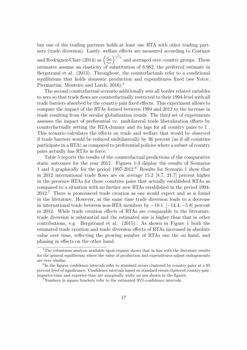
Table 5 reports the results of the counterfactual predictions of the comparativestatic outcomes for the year 2012. Figures 1-3 display the results of Scenarios1 and 3 graphically for the period 1997-2012.6 Results for Scenario 1 show thatin 2012 international trade flows are on average 15.2 [8.7, 21.7] percent higherin the presence RTAs for those countries pairs that actually established RTAs ascompared to a situation with no further new RTAs established in the period 1994-2012.7 There is pronounced trade creation as one would expect and as is foundin the literature. However, at the same time trade diversion leads to a decreasein international trade between non-RTA members by −10.1 [−14.4,−5.8] percentin 2012. While trade creation effects of RTAs are comparable to the literature,trade diversion is substantial and the estimated size is higher than that in othercontributions, e.g. Bergstrand et al. (2015). As shown in Figure 1 both theestimated trade creation and trade diversion effects of RTAs increased in absolutevalue over time, reflecting the growing number of RTAs one the on hand, andphasing in effects on the other hand.
5The robustness analysis available upon request shows that in line with the literature resultsfor the general equilibrium where the value of production and expenditures adjust endogenouslyare very similar.
6In the figures confidence intervals refer to standard errors clustered by country pairs at a 95percent level of significance. Confidence intervals based on standard errors clustered country-pair,importer-time and exporter-time are marginally wider an not shown in the figures.
7Numbers in square brackets refer to the estimated 95%-confidence intervals.
17
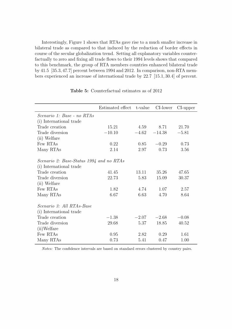
Interestingly, Figure 1 shows that RTAs gave rise to a much smaller increase inbilateral trade as compared to that induced by the reduction of border effects incourse of the secular globalization trend. Setting all explanatory variables counter-factually to zero and fixing all trade flows to their 1994 levels shows that comparedto this benchmark, the group of RTA members countries enhanced bilateral tradeby 41.5 [35.3, 47.7] percent between 1994 and 2012. In comparison, non-RTA mem-bers experienced an increase of international trade by 22.7 [15.1, 30.4] of percent.
Table 5: Counterfactual estimates as of 2012
Estimated effect t-value CI-lower CI-upper
Scenario 1: Base - no RTAs(i) International tradeTrade creation 15.21 4.59 8.71 21.70Trade diversion −10.10 −4.62 −14.38 −5.81(ii) WelfareFew RTAs 0.22 0.85 −0.29 0.73Many RTAs 2.14 2.97 0.73 3.56
Scenario 2: Base-Status 1994 and no RTAs(i) International tradeTrade creation 41.45 13.11 35.26 47.65Trade diversion 22.73 5.83 15.09 30.37(ii) WelfareFew RTAs 1.82 4.74 1.07 2.57Many RTAs 6.67 6.63 4.70 8.64
Scenario 3: All RTAs-Base(i) International tradeTrade creation −1.38 −2.07 −2.68 −0.08Trade diversion 29.68 5.37 18.85 40.52(ii)WelfareFew RTAs 0.95 2.82 0.29 1.61Many RTAs 0.73 5.41 0.47 1.00
Notes: The confidence intervals are based on standard errors clustered by country pairs.
18
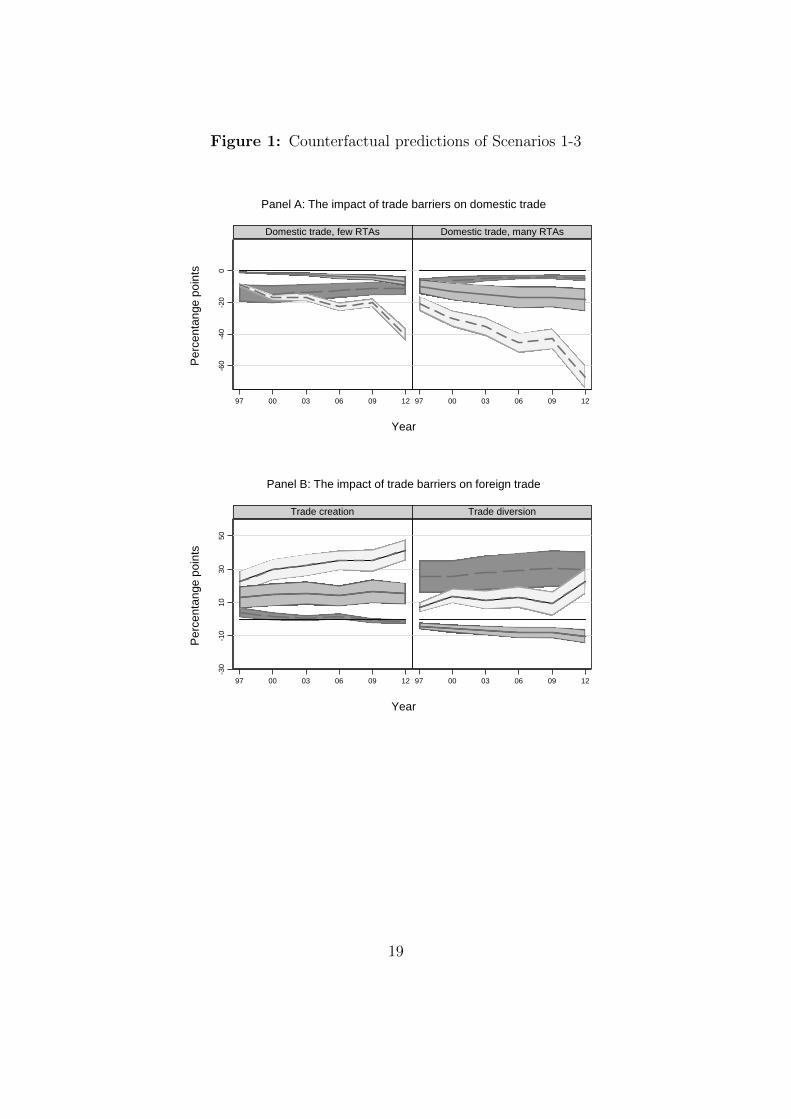
Figure 1: Counterfactual predictions of Scenarios 1-3
-60
-40
-20
0
97 00 03 06 09 12 97 00 03 06 09 12
Domestic trade, few RTAs Domestic trade, many RTAs
Pe
rce
nta
nge
po
ints
Year
Panel A: The impact of trade barriers on domestic trade-3
0-1
010
3050
97 00 03 06 09 12 97 00 03 06 09 12
Trade creation Trade diversion
Pe
rce
nta
nge
po
ints
Year
Panel B: The impact of trade barriers on foreign trade
-22
610
97 00 03 06 09 12 97 00 03 06 09 12
Few RTAs Many RTAs
All trade barriers, lower ci / All trade barriers, upper ci
RTA, lower ci / RTA, upper ci
All RTAs, lower ci / All RTAs, upper ci
Pe
rce
nta
nge
po
ints
Year
Note: Standard erros are clustered by country pairs
Panel C: Welfare effects
19
-60
-40
-20
0
97 00 03 06 09 12 97 00 03 06 09 12
Domestic trade, few RTAs Domestic trade, many RTAs
Pe
rce
nta
nge
po
ints
Year
Panel A: The impact of trade barriers on domestic trade
-30
-10
1030
50
97 00 03 06 09 12 97 00 03 06 09 12
Trade creation Trade diversion
Pe
rce
nta
nge
po
ints
Year
Panel B: The impact of trade barriers on foreign trade
-22
610
97 00 03 06 09 12 97 00 03 06 09 12
Few RTAs Many RTAs
All trade barriers, lower ci / All trade barriers, upper ci
RTA, lower ci / RTA, upper ci
All RTAs, lower ci / All RTAs, upper ci
Pe
rce
nta
nge
po
ints
Year
Note: Standard erros are clustered by country pairs
Panel C: Welfare effects
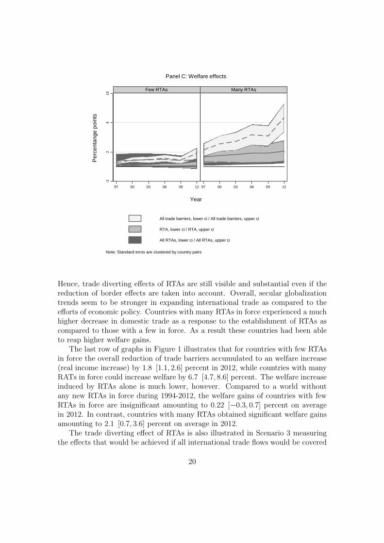
Hence, trade diverting effects of RTAs are still visible and substantial even if thereduction of border effects are taken into account. Overall, secular globalizationtrends seem to be stronger in expanding international trade as compared to theefforts of economic policy. Countries with many RTAs in force experienced a muchhigher decrease in domestic trade as a response to the establishment of RTAs ascompared to those with a few in force. As a result these countries had been ableto reap higher welfare gains.
The last row of graphs in Figure 1 illustrates that for countries with few RTAsin force the overall reduction of trade barriers accumulated to an welfare increase(real income increase) by 1.8 [1.1, 2.6] percent in 2012, while countries with manyRATs in force could increase welfare by 6.7 [4.7, 8.6] percent. The welfare increaseinduced by RTAs alone is much lower, however. Compared to a world withoutany new RTAs in force during 1994-2012, the welfare gains of countries with fewRTAs in force are insignificant amounting to 0.22 [−0.3, 0.7] percent on averagein 2012. In contrast, countries with many RTAs obtained significant welfare gainsamounting to 2.1 [0.7, 3.6] percent on average in 2012.
The trade diverting effect of RTAs is also illustrated in Scenario 3 measuringthe effects that would be achieved if all international trade flows would be covered
20
by a RTA and the spaghetti bowl of RTAs is eliminated. In this scenario tradeflows that currently are not covered by an RTA would increase by 29.7 [18.9, 40.5]percent as compared to 1994, while trade flows that are covered by RTAs wouldmarginally decrease, −1.4 [−2.7, 0.1] percent. The involved welfare effects pointto an increase of 1.0 [0.3, 1.6] for countries with few RTAs and to 0.8 [0.5, 1.0]percent for those with many. All these estimates are significant at the 5 percentlevel. Hence, it seems the currently observed spaghetti bowl induced by RTAs doesby far not exhaust possible welfare gains of trade liberalization.
While the trade creating and trade diverting effects of RTAs as well as theirwelfare effects are significant in almost all cases, there is substantial uncertaintyinduced by parameter estimation. Despite rather precisely estimated direct RTAeffects, the counterfactual predictions exhibit quite large confidence intervals. Thisissue seems to be overlooked in many applications that evaluate RTA effects.
5 Conclusions
PPML panel estimation of gravity models potentially involves a huge set of dum-mies. Even if one wipes out country-pair fixed effects and uses zig-zag algorithmsto handle country-pair, exporter-time and importer-time fixed effects to obtainconsistently estimated structural paper in high dimensional panel models, econo-metric issues remain. Proper inference for parameter estimates and counterfactualpredictions needs robust and unbiased estimates of the standard errors of the es-timated structural parameters that are unaffected by the incidental parametersproblem. The present contribution proposes a constrained panel PPML estima-tor as an alternative to bootstrapping. This estimator exploits the restrictionsimposed by the multilateral system of trade resistances for both estimation andcounterfactual prediction. In this setting all dummies, including the fixed countrypair-effects, are functionally determined by the structural slope parameters. Thisestimation procedure works well and estimated standard errors reveal only neg-ligible bias. The delta method delivers reliable standard errors of counterfactualpredictions and welfare effects. Monte Carlo simulations confirm this view.
Applying the constrained panel PPML estimator to a panel of bilateral traderelationship of 65 countries for the period 1994-2012 illustrates the usefulness ofthis estimation procedure. Estimates indicate a secular trend in globalization thatinduced a pronounced deterioration of border effects. At the same time manyRTAs came into force that led to substantial trade creation. The cost is trade di-version elsewhere. The estimated trade diversion effects induced by adjustment ofmultilateral resistances turn out significant and substantial. However the spaghettibowl of RTA relationships by far does not exhaust the potential welfare gains ofmultilateral trade liberalization. A multilateral trade liberalization effort would
21

remove the trade diverting effects, while only marginally reducing internationaltrade flows between country-pairs that actually have RTAs in force.
22
References
Allen, T., C. Arkolakis and Y. Takahashi (2017), Universal Gravity, NBER Work-ing Paper 20787.
Anderson, J.E. and E. van Wincoop (2003), Gravity with Gravitas: A Solutionto the Border Puzzle, American Economic Review 93(1), 170-192.
Anderson, J. E. and Y.V. Yotov (2016), Terms of Trade and Global EfficiencyEffects of Free Trade Agreements, 1990–2002, Journal of International Eco-nomics 99, 279–298.
Arvis, J.-F. and B. Shepherd (2013), The Poisson Quasi-Maximum Likelihood Es-timator: A Solution to the ‘Adding up’ Problem in Gravity Models, AppliedEconomic Letters 20(6), 515–519.
Baier, S. L., and J.H. Bergstrand (2007), Do Free Trade Agreements ActuallyIncrease Members’ International Trade?, Journal of international Economics71(1), 72-95.
Bergstrand, J.H., M. Larch, and Y.V. Yotov (2015), Economic Integration Agree-ments, Border Effects, and Distance Elasticities in the Gravity Equation,European Economic Review 78(), 307-327.
Bergstrand, J.H., P.H. Egger and M. Larch (2013), Gravity Redux: Estimationof Gravity-equation Coefficients, Elasticities of Substitution, and GeneralEquilibrium Comparative Statics under Asymmetric Bilateral Trade Costs,Journal of International Economics 89(1), 110-121.
Blundell, R., R. Griffith and F. Windmeijer (2002), Individual Effects and Dy-namics in Count Data Models, Journal of Econometrics 108(1), 113–131.
Borchert, I., and Y.V. Yotov (2017), Distance, Globalization, and InternationalTrade, Economics Letters 153, 32–38.
Caliendo, L. and F. Parro, F. (2015), Estimates of the Trade and Welfare Effectsof NAFTA, The Review of Economic Studies 82(1), 1–44.
Cameron, C.A, J. B. Gelbach and D. L. Miller (2011), Robust Inference WithMultiway Clustering, Journal of Business and Economic Statistics 29(2),238-249.
Clausing, K. A. (2001), Trade Creation and Trade diversion in the Canada?UnitedStates Free Trade Agreement, Canadian Journal of Economics/Revue cana-dienne d’economique 34(3), 677–696.
23
Costinot, A. and A. Rodrıguez-Clare (2014), Trade Theory with Numbers: Quan-tifying the Consequences of Globalization. Chapter 4 in Gopinath, G, E.Helpman and K. S. Rogooff (eds), Handbook of International EconomicsVol. 4, Elsevier, Oxford, 197–261.
Dai M., Y.V. Yotov and T. Zylkin (2014), On the Trade-Diversion Effects of FreeTrade Agreements, Economics Letters 122, 321–325.
De Sousa J., Mayer, T. and S. Zignago (2012), Market Access in Global andRegional Trade, Regional Science and Urban Economics, 42(6), 1037–1152.
Eaton, J. and S. Kortum (2002), Technology, Geography, and Trade, Economet-rica 70(5), 1741-1779.
Egger, P.H. and M. Larch (2008), Interdependent Preferential Trade AgreementMemberships: An Empirical Analysis, Journal of International Economics76(2), 384–399.
Egger, P.H. and F. Tarlea (2015), Multi-way Clustering Estimation of StandardErrors in Gravity Models, Economic Letters 134, 144–147.
Fally, T. (2015), Structural Gravity and Fixed Effects, Journal of InternationalEconomics 97(1), 76–85.
Falocci, N.,R. Paniccia and E. Stanghellini (2009), Regression Modelling of theFlows in an Input–Output Table with Accounting Constraints, StatisticalPapers 50(2), 373–382.
Felbermayr, G., B. Heid, M., Larch and E. Yalcin (2015), Macroeconomic Poten-tials of Transatlantic Free Trade: A High Resolution Perspective for Europeand the World, Economic Policy 30(83), 491-537.
Figueiredo, O., P. Guimaraes, P. and D. Woodward (2015), Industry Localization,Distance Decay, and Knowledge Spillovers: Following the Patent Paper Trail,Journal of Urban Economics 89, 21–31.
Freund, C. and E. Ornelas (2010), Regional Trade Agreements, Annual Reviewof Economics 2(1), 139–166.
Guimaraes, P. and P. Portugal (2010), A Simple Feasible Procedure to Fit ModelsWith high-dimensional Fixed Effects, The Stata Journal 10(4), 628–649.
Hausman, J., B.H. Hall and Z. Griliches (1984), Econometric Models for CountData with an Application to the Patents-R&D Relationship, Econometrica52(4), 909–938.
24

Head K. and T. Mayer (2014), Gravity Equations: Workhorse, Toolkit, and Cook-book. Chapter 3 in Gopinath, G, E. Helpman and K. S. Rogooff (eds),Handbook of International Economics Vol. 4, Elsevier, Oxford, 131–195.
Heyde, C.C. and R. Morton (1993), On Constrained Quasi-Likelihood Estimation,Biometrika 80(4), 755–761.
Magee, C. S. (2008), New Measures of Trade Creation and Trade diversion, Jour-nal of International Economics 75(2), 349-362.
Magee, C. S. (2016), Trade creation, Trade diversion, and the General EquilibriumEffects of Regional trade Agreements: A Study of the European Community–Turkey Customs Union, Review of World Economics 152(2), 383–399.
Mayer, T. and Zignago, S. (2011), Notes on CEPII’s distances measures: theGeoDist Database, CEPII Working Paper 2011-25.
Newey, W. K. and D. L. McFadden (1994). Large Sample Estimation and Hypoth-esis Testing, in Engle R. F. and D. McFadden (eds.), Handbook of Econo-metrics. Vol. 4., Elsevier Science, Amsterdam.
Nicita, A. and M. Olarreaga (2007), Trade, Production and Protection 1976-2004,World Bank Economic Review 21(1), 165–71.
Palmgren, J. (1981), The Fisher Information Matrix for Log Linear Models Ar-guing Conditionally on Observed Explanatory Variables, Biometrika 68(2),563-566.
Pfaffermayr, M. (2017), Constrained Poisson Pseudo Maximum Likelihood Esti-mation of Structural Gravity Models, unpublished manuscript.
Santos Silva, J.M.C. and F.A.G Windmeijer (1997), Endogeneity in Count DataModels: An Application to Demand for Health Care, Journal of AppliedEconometrics 12(3), 281–294.
Smyth, G.K. (1996), Partitioned Algorithms for Maximum Likelihood and otherNon-linear Estimation, Statistics and Computing 6(3), 201–216.
Sorgho, Z. (2016), RTAs’ Proliferation and Trade-diversion Effects: Evidence ofthe ‘Spaghetti’ Bowl Phenomenon, The World Economy 39(2), 285–300.
Trefler, D.(2004), The Long and Short of the Canadian-U.S. Free Trade Agree-ment, American Economic Review 94(4), 870–895.
25
Van Garderen, J.K. and C. Shah (2002), Exact Interpretation of Dummy Vari-ables in Semilogarithmic Equations, The Econometrics Journal 5(1), 149–159.
Wooldridge, J. (1997), Quasi-Likelihood Methods for Count Data, in PesaranH. and P. Schmidt (eds.), Handbook of Applied Econometrics Volume II:Micro-economics, Blackwell, Oxford UK.
Wooldridge, J. (1999), Distribution-free Estimation of Some Nonlinear PanelData Models, Journal of International Economics, 90(1), 77–97.
Yotov, Y.V. (2012), A Simple Solution to the Distance Puzzle in InternationalTrade, Economics Letters 117(3) 794–798.
Yotov, Y.V., R. Piermartini, J.A. Monteiro and Larch, M. (2016). An AdvancedGuide to Trade Policy Analysis: The Structural Gravity Model. World TradeOrganization, Geneva.
26
Appendix (intended to be published as a supplement)
A Constrained PPML-estimation in three-way
panels
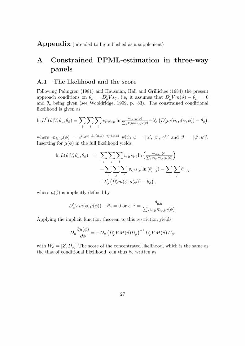
A.1 The likelihood and the score
Following Palmgren (1981) and Hausman, Hall and Grilliches (1984) the presentapproach conditions on θµ = D′µV sC , i.e, it assumes that D′µV m(ϑ) − θµ = 0and θµ being given (see Wooldridge, 1999, p. 83). The constrained conditionallikelihood is given as
lnLC(ϑ|V, θµ, θφ) =∑i
∑j
∑t
vijtsijt lnmφ,ijt(φ)∑
s vijtmφ,ijs(φ)−λ′φ
(D′φm(φ, µ(α, φ))− θφ
),
where mijt,φ(φ) = ez′ijtα+βit(α,µ)+γjt(α,µ) with φ = [α′, β′, γ′]′ and ϑ = [φ′, µ′]′.
Inserting for µ(φ) in the full likelihood yields
lnL(ϑ|V, θµ, θφ) =∑i
∑j
∑t
vijtsijt ln(
mφ,ijt(φ)∑s vijtmφ,ijs(φ)
)+∑i
∑j
∑t
vijtsijt ln (θµ,ij)−∑i
∑j
θµ,ij
+λ′φ(D′φm(φ, µ(φ))− θφ
),
where µ(φ) is implicitly defined by
D′µV m(φ, µ(φ))− θµ = 0 or eµij =θµ,it∑
t vijtmφ,ijt(φ).
Applying the implicit function theorem to this restriction yields
Dµ∂µ(φ)
∂φ= −Dµ
(D′µVM(ϑ)Dµ
)−1D′µVM(ϑ)Wφ,
with Wφ = [Z,Dφ]. The score of the concentrated likelihood, which is the same asthe that of conditional likelihood, can thus be written as
27

∂ lnL(ϑ|V, θ, µ)
∂φ=
∑i
∑j
∑t
[sijt −mijt(φ, µij(φ)]
(wφ,ijt +
∂µij(φ)
∂φ′
)
+
(Wφ +Dµ
∂µ(φ)
∂φ′
)′M(ϑ)Dφλφ
= W ′φ
(ITC2 −M(ϑ)V Dµ
(D′µVM(ϑ)Dµ
)−1D′µ
)︸ ︷︷ ︸
Qµ(ϑ)
∗ (V (s−m(ϑ)) +M(ϑ)Dφλφ) .
Qµ(ϑ) is a projection matrix with D′µQµ(ϑ) = 0. Qµ(ϑ) is not symmetric asQµ(ϑ)Dµ 6= 0. Since V m(ϑ) = 1
TM(ϑ)V Dµι(C−1)2 it follows thatW ′
φQµ(ϑ)V ′m(ϑ) =
0. The score of the constrained conditional likelihood is solved at ϑ and can thusbe written as
∂ lnL(ϑ|V, θ)∂φ
= W ′φQµ(ϑ)V s+W ′
φQµ(ϑ)M(ϑ)Dφλφ
∂ lnL(ϑ|V, θ)∂λ
= Dφm(ϑ)− θµ.
The score of the Lagrangian of the constrained likelihood of the full model is givenas
∂ lnLC(ϑ|V, θC)
∂α= Z ′V (s−m(ϑ)) + Z ′M(ϑ)V Dµλµ + Z ′M(ϑ)Dφλφ
∂ lnLC(ϑ|V, θC)
∂µ= D′µV (s−m(ϑ)) +D′µM(ϑ)V Dµλµ +D′µM(ϑ)Dφλφ
∂ lnLC(ϑ|V, θC)
∂φC= D′φV (s−m(ϑ)) +D′φM(ϑ)V Dµλµ +D′φM(ϑ)Dφλφ
∂ lnLC(ϑ|V, θC)
∂λµ= θµ −D′µV m(ϑ)
∂ lnLC(ϑ|V, θC)
∂λφ= θφ −D′φm(ϑ)
28
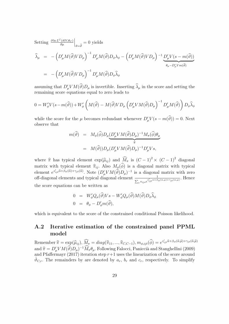
Setting ∂ lnLC(ϑ|V,θC)∂µ
∣∣∣ϑ=ϑ
= 0 yields
λµ = −(D′µM(ϑ)V Dµ
)−1D′µM(ϑ)Dφλφ −
(D′µM(ϑ)V Dµ
)−1D′µV (s−m(ϑ))︸ ︷︷ ︸
θµ−D′µV m(ϑ)
= −(D′µM(ϑ)V Dµ
)−1D′µM(ϑ)Dφλφ
assuming that D′µVM(ϑ)Dµ is invertible. Inserting λµ in the score and setting theremaining score equations equal to zero leads to
0 = W ′φV (s−m(ϑ))+W ′
φ
(M(ϑ)−M(ϑ)V Dµ
(D′µVM(ϑ)Dµ
)−1D′µM(ϑ)
)Dφλφ
while the score for the µ becomes redundant whenever D′µV (s−m(ϑ)) = 0. Nextobserve that
m(ϑ) = Mφ(φ)Dµ(D′µVM(ϑ)Dµ)−1Mπ(φ)θµ︸ ︷︷ ︸π
= M(ϑ))Dµ(D′µVM(ϑ)Dµ)−1D′µV s,
where π has typical element exp(µij) and Mπ is (C − 1)2× (C − 1)2 diagonal
matrix with typical element πij. Also Mφ(φ) is a diagonal matrix with typical
element ez′ijtα+βit(α)+γjt(α). Note (D′µVM(ϑ)Dµ)−1 is a diagonal matrix with zero
off-diagonal elements and typical diagonal element 1∑s vijse
z′ijtα+βit(α,µ)+γjt(α,µ)
. Hence
the score equations can be written as
0 = W ′φQµ(ϑ)V s−W ′
φQµ(ϑ)M(ϑ)Dφλφ
0 = θφ −D′φm(ϑ),
which is equivalent to the score of the constrained conditional Poisson likelihood.
A.2 Iterative estimation of the constrained panel PPMLmodel
Remember π = exp(µij), Mπ = diag(π11, ..., πC,C−1), mφ,ijt(φ) = ez′ijtα+βit(α,µ)+γjt(α,µ)
and π = D′µVM(ϑ)Dµ)−1Mπθµ. Following Falocci, Paniccia and Stanghellini (2009)and Pfaffermayr (2017) iteration step r+1 uses the linearization of the score aroundϑC,r. The remainders by are denoted by ar, br and cr, respectively. To simplify
29
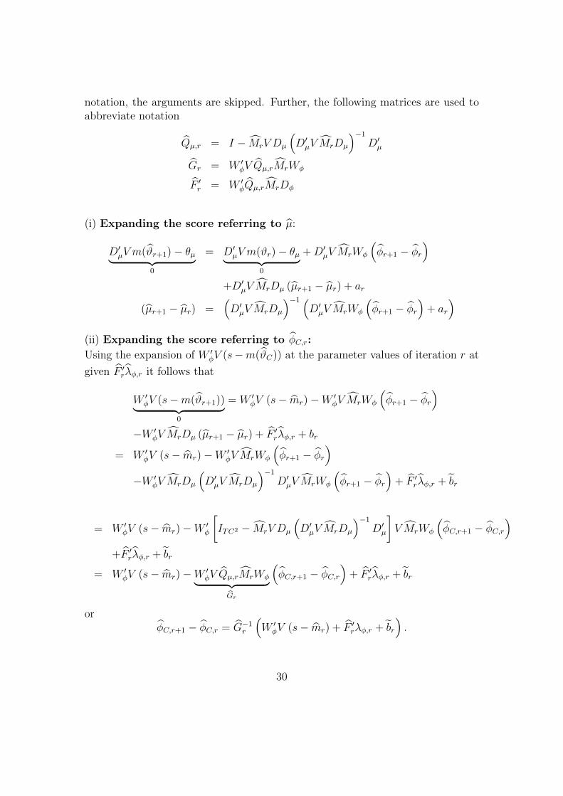
notation, the arguments are skipped. Further, the following matrices are used toabbreviate notation
Qµ,r = I − MrV Dµ
(D′µV MrDµ
)−1D′µ
Gr = W ′φV Qµ,rMrWφ
F ′r = W ′φQµ,rMrDφ
(i) Expanding the score referring to µ:
D′µV m(ϑr+1)− θµ︸ ︷︷ ︸0
= D′µV m(ϑr)− θµ︸ ︷︷ ︸0
+D′µV MrWφ
(φr+1 − φr
)+D′µV MrDµ (µr+1 − µr) + ar
(µr+1 − µr) =(D′µV MrDµ
)−1 (D′µV MrWφ
(φr+1 − φr
)+ ar
)(ii) Expanding the score referring to φC,r:
Using the expansion of W ′φV (s−m(ϑC)) at the parameter values of iteration r at
given F ′rλφ,r it follows that
W ′φV (s−m(ϑr+1))︸ ︷︷ ︸
0
= W ′φV (s− mr)−W ′
φV MrWφ
(φr+1 − φr
)−W ′
φV MrDµ (µr+1 − µr) + F ′rλφ,r + br
= W ′φV (s− mr)−W ′
φV MrWφ
(φr+1 − φr
)−W ′
φV MrDµ
(D′µV MrDµ
)−1D′µV MrWφ
(φr+1 − φr
)+ F ′rλφ,r + br
= W ′φV (s− mr)−W ′
φ
[ITC2 − MrV Dµ
(D′µV MrDµ
)−1D′µ
]V MrWφ
(φC,r+1 − φC,r
)+F ′rλφ,r + br
= W ′φV (s− mr)−W ′
φV Qµ,rMrWφ︸ ︷︷ ︸Gr
(φC,r+1 − φC,r
)+ F ′rλφ,r + br
orφC,r+1 − φC,r = G−1r
(W ′φV (s− mr) + F ′rλφ,r + br
).
30
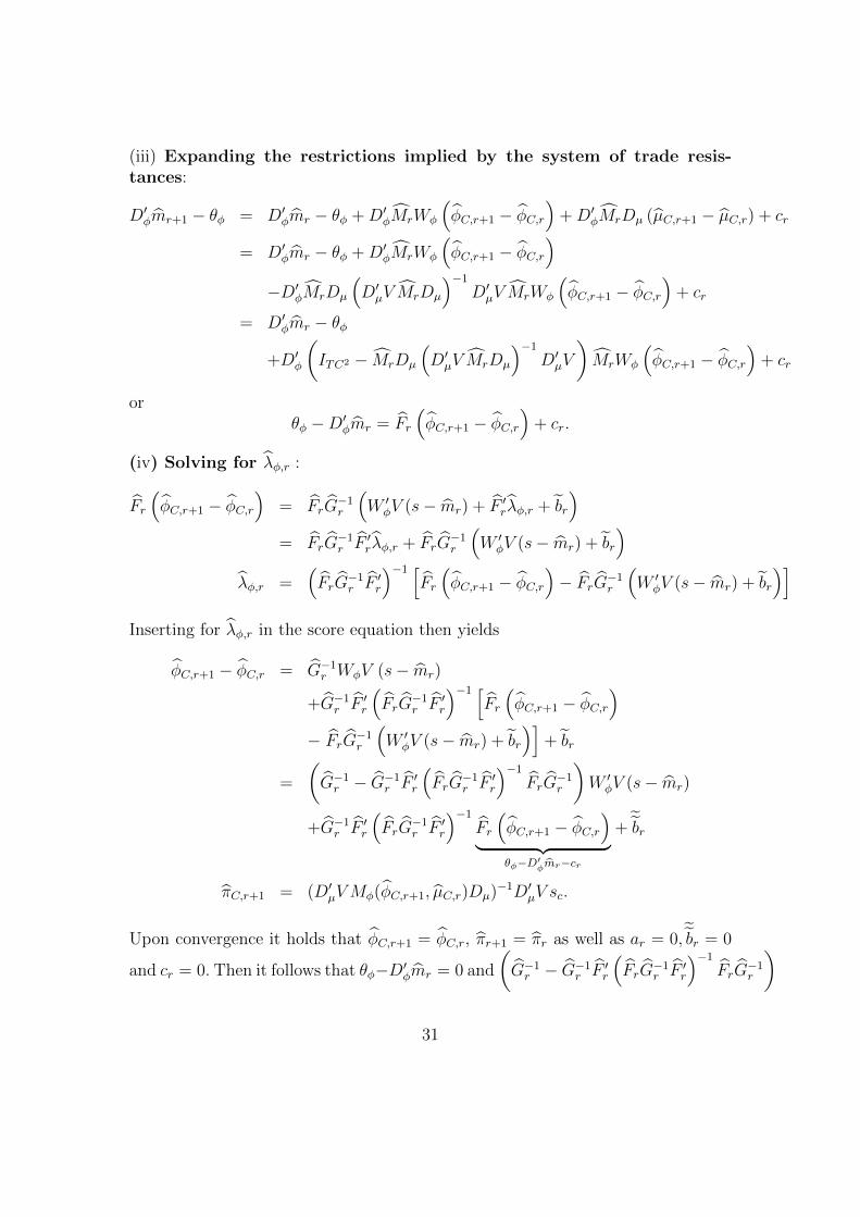
(iii) Expanding the restrictions implied by the system of trade resis-tances:
D′φmr+1 − θφ = D′φmr − θφ +D′φMrWφ
(φC,r+1 − φC,r
)+D′φMrDµ (µC,r+1 − µC,r) + cr
= D′φmr − θφ +D′φMrWφ
(φC,r+1 − φC,r
)−D′φMrDµ
(D′µV MrDµ
)−1D′µV MrWφ
(φC,r+1 − φC,r
)+ cr
= D′φmr − θφ
+D′φ
(ITC2 − MrDµ
(D′µV MrDµ
)−1D′µV
)MrWφ
(φC,r+1 − φC,r
)+ cr
orθφ −D′φmr = Fr
(φC,r+1 − φC,r
)+ cr.
(iv) Solving for λφ,r :
Fr
(φC,r+1 − φC,r
)= FrG
−1r
(W ′φV (s− mr) + F ′rλφ,r + br
)= FrG
−1r F ′rλφ,r + FrG
−1r
(W ′φV (s− mr) + br
)λφ,r =
(FrG
−1r F ′r
)−1 [Fr
(φC,r+1 − φC,r
)− FrG−1r
(W ′φV (s− mr) + br
)]Inserting for λφ,r in the score equation then yields
φC,r+1 − φC,r = G−1r WφV (s− mr)
+G−1r F ′r
(FrG
−1r F ′r
)−1 [Fr
(φC,r+1 − φC,r
)− FrG−1r
(W ′φV (s− mr) + br
)]+ br
=
(G−1r − G−1r F ′r
(FrG
−1r F ′r
)−1FrG
−1r
)W ′φV (s− mr)
+G−1r F ′r
(FrG
−1r F ′r
)−1Fr
(φC,r+1 − φC,r
)︸ ︷︷ ︸
θφ−D′φmr−cr
+˜br
πC,r+1 = (D′µVMφ(φC,r+1, µC,r)Dµ)−1D′µV sc.
Upon convergence it holds that φC,r+1 = φC,r, πr+1 = πr as well as ar = 0,˜br = 0
and cr = 0. Then it follows that θφ−D′φmr = 0 and
(G−1r − G−1r F ′r
(FrG
−1r F ′r
)−1FrG
−1r
)
31
∗W ′φV (s − mr) = 0 (see Newey and McFadden, 1994, p. 2219 and the projection
estimator of Heyde and Morton 1993, p. 756).
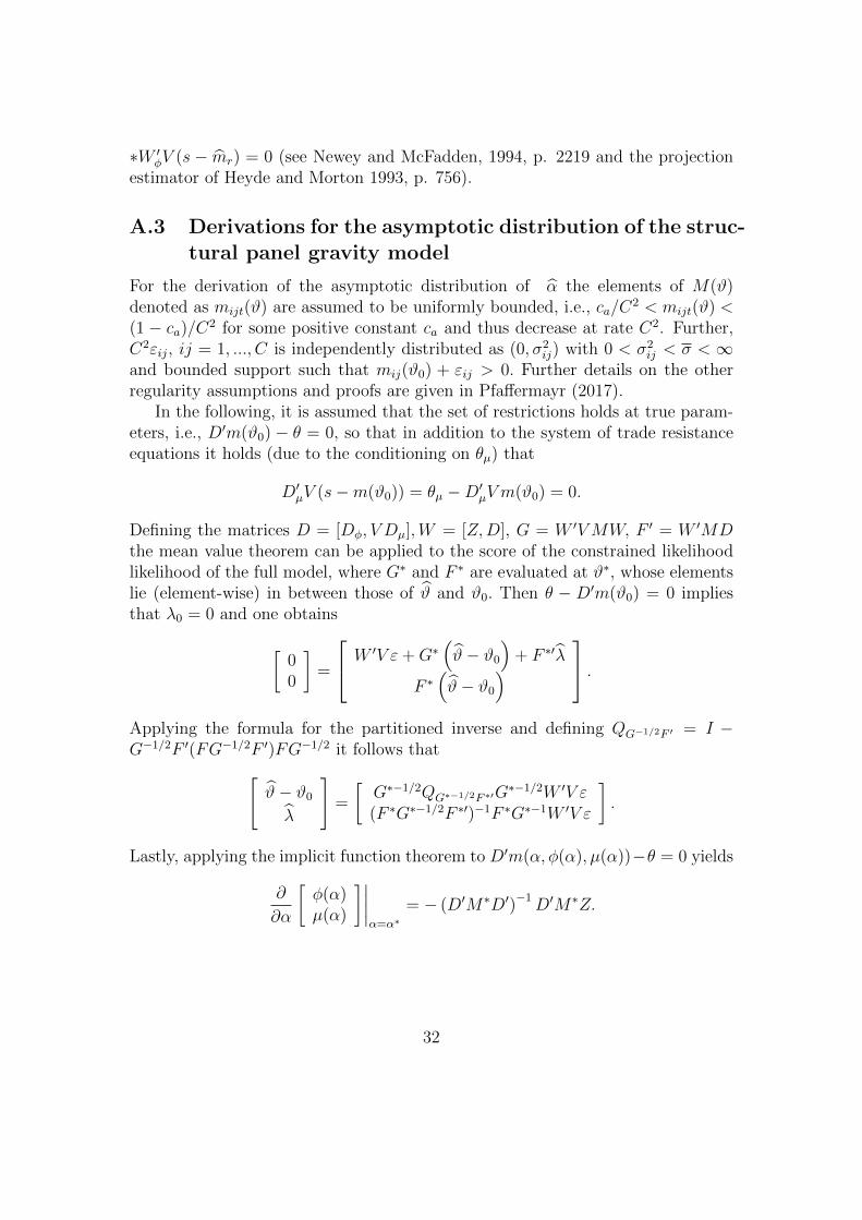
A.3 Derivations for the asymptotic distribution of the struc-tural panel gravity model
For the derivation of the asymptotic distribution of α the elements of M(ϑ)denoted as mijt(ϑ) are assumed to be uniformly bounded, i.e., ca/C
2 < mijt(ϑ) <(1 − ca)/C2 for some positive constant ca and thus decrease at rate C2. Further,C2εij, ij = 1, ..., C is independently distributed as (0, σ2
ij) with 0 < σ2ij < σ < ∞
and bounded support such that mij(ϑ0) + εij > 0. Further details on the otherregularity assumptions and proofs are given in Pfaffermayr (2017).
In the following, it is assumed that the set of restrictions holds at true param-eters, i.e., D′m(ϑ0) − θ = 0, so that in addition to the system of trade resistanceequations it holds (due to the conditioning on θµ) that
D′µV (s−m(ϑ0)) = θµ −D′µV m(ϑ0) = 0.
Defining the matrices D = [Dφ, V Dµ],W = [Z,D], G = W ′VMW, F ′ = W ′MDthe mean value theorem can be applied to the score of the constrained likelihoodlikelihood of the full model, where G∗ and F ∗ are evaluated at ϑ∗, whose elementslie (element-wise) in between those of ϑ and ϑ0. Then θ − D′m(ϑ0) = 0 impliesthat λ0 = 0 and one obtains
[00
]=
W ′V ε+G∗(ϑ− ϑ0
)+ F ∗′λ
F ∗(ϑ− ϑ0
) .Applying the formula for the partitioned inverse and defining QG−1/2F ′ = I −G−1/2F ′(FG−1/2F ′)FG−1/2 it follows that[
ϑ− ϑ0
λ
]=
[G∗−1/2QG∗−1/2F ∗′G
∗−1/2W ′V ε(F ∗G∗−1/2F ∗′)−1F ∗G∗−1W ′V ε
].
Lastly, applying the implicit function theorem to D′m(α, φ(α), µ(α))−θ = 0 yields
∂
∂α
[φ(α)µ(α)
]∣∣∣∣α=α∗
= − (D′M∗D′)−1D′M∗Z.
32

Hence, one obtains
ϑ− ϑ0 =(IK+(C−1)2+(2C−1)T − (D′M∗D′)
−1D′M∗Z
)(α− α0)
and
G∗[
IK− (D′M∗D′)−1D′M∗Z
](α− α0) = G∗1/2QG∗−1/2F ∗′G
∗−1/2W ′V ε.
Multiplying from left by [IK×K , 0K×C(C−1)+(2C−1)T ], shows that
[IK×K , 0K×C(C−1)+(2C−1)T ]G∗ (α− α0)
= [IK×K , 0K×C(C−1)+(2C−1)T ]
[Z ′VM∗V Z − Z ′VM∗V D (D′M0D)−1D′M0Z
D′VM∗V Z −D′VM∗V D (D′M0D)−1D′M0Z
](α− α0)
= Z ′V(M∗ −M∗D(D′M∗D)−1D′M∗)Z (α− α0) .
and
[IK×K , 0K×C(C−1)+(2C−1)T ]
([IK 00 IC(C−1)+(2C−1)T
]− F ∗′
(F ∗G∗−1F ∗′
)−1F ∗G∗−1
)W ′V ε
= Z ′(ITC2 −M∗D
(F ∗G∗−1F ∗′
)−1F ∗G∗−1W ′
)V ε.
since
[IK×K , 0K×C(C−1)+(2C−1)T ]F ∗′= [IK×K , 0K×C(C−1)+(2C−1)T ]
[Z ′
D′
]M∗D = Z ′M∗D.
In the notation of Proposition 2 in Pfaffermayr (2017) one thus obtains
A(α) = TC2Z ′(ITC2 −M(α)D′(F (α)G(α)−1F (α)′
)−1F (α)G(α)−1W ′)V
B(α) = Z ′V[M(α)−M(α)D(D′M(α)D)−1D′M(α)
]Z.
A.4 Comparative statics
We define the selection matrix R so that RM(α,Z)−1 has typical non-zero diagonalelement mij(α,zij)
−1 and
Λ(α) = RM(α,Z)−1m(α,Zc)
33
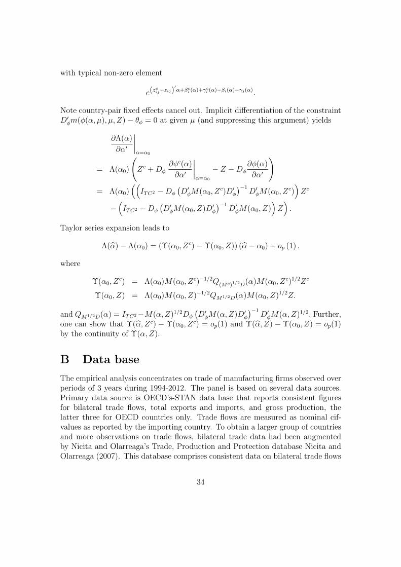
with typical non-zero element
e(zcij−zij)
′α+βci (α)+γ
ci (α)−βi(α)−γj(α).
Note country-pair fixed effects cancel out. Implicit differentiation of the constraintD′φm(φ(α, µ), µ, Z)− θφ = 0 at given µ (and suppressing this argument) yields
∂Λ(α)
∂α′
∣∣∣∣α=α0
= Λ(α0)
(Zc +Dφ
∂φc(α)
∂α′
∣∣∣∣α=α0
− Z −Dφ∂φ(α)
∂α′
)= Λ(α0)
((ITC2 −Dφ
(D′φM(α0, Z
c)D′φ)−1
D′φM(α0, Zc))Zc
−(ITC2 −Dφ
(D′φM(α0, Z)D′φ
)−1D′φM(α0, Z)
)Z).
Taylor series expansion leads to
Λ(α)− Λ(α0) = (Υ(α0, Zc)−Υ(α0, Z)) (α− α0) + op (1) .
where
Υ(α0, Zc) = Λ(α0)M(α0, Z
c)−1/2Q(Mc)1/2D(α)M(α0, Zc)1/2Zc
Υ(α0, Z) = Λ(α0)M(α0, Z)−1/2QM1/2D(α)M(α0, Z)1/2Z.
and QM1/2D(α) = ITC2−M(α,Z)1/2Dφ
(D′φM(α,Z)D′φ
)−1D′φM(α,Z)1/2. Further,
one can show that Υ(α, Zc) − Υ(α0, Zc) = op(1) and Υ(α, Z) − Υ(α0, Z) = op(1)
by the continuity of Υ(α,Z).
B Data base
The empirical analysis concentrates on trade of manufacturing firms observed overperiods of 3 years during 1994-2012. The panel is based on several data sources.Primary data source is OECD’s-STAN data base that reports consistent figuresfor bilateral trade flows, total exports and imports, and gross production, thelatter three for OECD countries only. Trade flows are measured as nominal cif-values as reported by the importing country. To obtain a larger group of countriesand more observations on trade flows, bilateral trade data had been augmentedby Nicita and Olarreaga’s Trade, Production and Protection database Nicita andOlarreaga (2007). This database comprises consistent data on bilateral trade flows
34
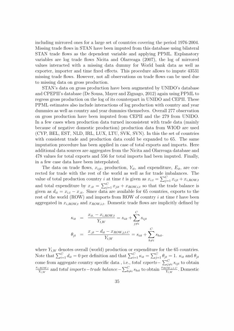
including mirrored ones for a large set of countries covering the period 1976-2004.Missing trade flows in STAN have been imputed from this database using bilateralSTAN trade flows as the dependent variable and applying PPML. Explanatoryvariables are log trade flows Nicita and Olarreaga (2007), the log of mirroredvalues interacted with a missing data dummy for World bank data as well asexporter, importer and time fixed effects. This procedure allows to impute 43531missing trade flows. However, not all observations on trade flows can be used dueto missing data on gross production.
STAN’s data on gross production have been augmented by UNIDO’s databaseand CPEPII’s database (De Sousa, Mayer and Zignago, 2012) again using PPML toregress gross production on the log of its counterpart in UNIDO and CEPII. ThesePPML estimates also include interactions of log production with country and yeardummies as well as country and year dummies themselves. Overall 277 observationon gross production have been imputed from CEPII and the 279 from UNIDO.In a few cases when production data turned inconsistent with trade data (mainlybecause of negative domestic production) production data from WIOD are used(CYP, BEL, EST, NLD, IRL, LUX, LTU, SVK, SVN). In this the set of countrieswith consistent trade and production data could be expanded to 65. The sameimputation procedure has been applied in case of total exports and imports. Hereadditional data sources are aggregates from the Nicita and Olarreaga database and478 values for total exports and 556 for total imports had been imputed. Finally,in a few case data have been interpolated.
The data on trade flows, xijt, production, Yit, and expenditure, Eit, are cor-rected for trade with the rest of the world as well as for trade imbalances. Thevalue of total production country i at time t is given as xi.t =
∑Cj=1 xijt + xi,ROW,t
and total expenditure by x.it =∑C
j=1 xjit + xROW,i,t so that the trade balance isgiven as dit = xi.t − x.it. Since data are available for 65 countries, exports to therest of the world (ROW) and imports from ROW of country i at time t have beenaggregated in xi,ROW,t and xROW,i,t. Domestic trade flows are implicitly defined by
κit =xit. − xi,ROW,t
Yt,W= siit +
C∑j 6=i
sijt
θjt =x.jt − dit − xROW,j,t.C
Yt,W= siit +
C∑h6=i
shit.
where Yt,W denotes overall (world) production or expenditure for the 65 countries.
Note that∑C
i=1 dit = 0 per definition and that∑C
i=1 κit =∑C
j=1 θjt = 1. κit and θjt
come from aggregate country specific data , i.e., total exports−∑C
j 6=i sijt to obtainxi,ROW,tYt,W
and total imports−trade balance−∑C
h6=i shit to obtainxROW,j,t.C
Yt,W. Domestic
35

trade is derived as total production− total exports using the unilateral data, whileinternational trade comes from the bilateral trade data. Due to missing trade andmeasurement errors in the bilateral trade data the aggregation of sijt to domesticproduction κit and domestic expenditures θjt is not exact, however.
36
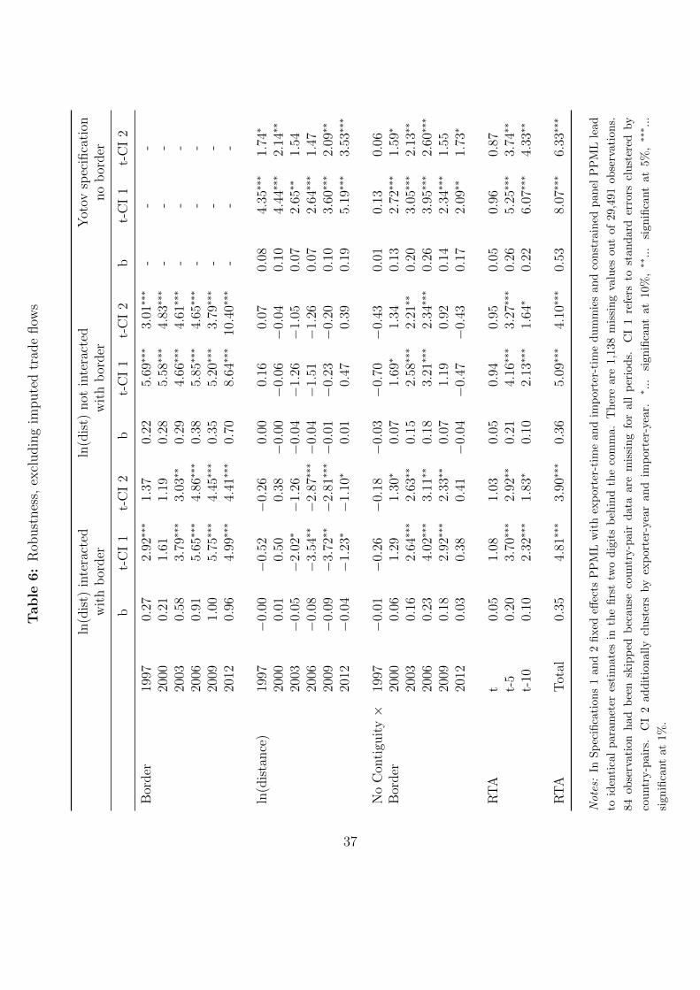
Table
6:
Rob
ust
nes
s,ex
cludin
gim
pute
dtr
ade
flow
s
ln(d
ist)
inte
ract
edln
(dis
t)not
inte
ract
edY
otov
spec
ifica
tion
wit
hb
order
wit
hb
order
no
bor
der
bt-
CI
1t-
CI
2b
t-C
I1
t-C
I2
bt-
CI
1t-
CI
2
Bor
der
1997
0.27
2.92∗∗∗
1.37
0.22
5.69∗∗∗
3.01∗∗∗
--
-20
000.
211.
611.
190.
285.
58∗∗∗
4.83∗∗∗
--
-20
030.
583.
79∗∗∗
3.03∗∗
0.29
4.66∗∗∗
4.61∗∗∗
--
-20
060.
915.
65∗∗∗
4.86∗∗∗
0.38
5.85∗∗∗
4.65∗∗∗
--
-20
091.
005.
75∗∗∗
4.45∗∗∗
0.35
5.20∗∗∗
3.79∗∗∗
--
-20
120.
964.
99∗∗∗
4.41∗∗∗
0.70
8.64∗∗∗
10.4
0∗∗∗
--
-
ln(d
ista
nce
)19
97−
0.00
−0.
52−
0.26
0.00
0.16
0.07
0.08
4.35∗∗∗
1.74∗
2000
0.01
0.50
0.38
−0.
00−
0.06
−0.
040.
104.
44∗∗∗
2.14∗∗
2003
−0.
05−
2.02∗−
1.26
−0.
04−
1.26
−1.
050.
072.
65∗∗
1.54
2006
−0.
08−
3.54∗∗−
2.87∗∗∗−
0.04
−1.
51−
1.26
0.07
2.64∗∗∗
1.47
2009
−0.
09−
3.72∗∗−
2.81∗∗∗−
0.01
−0.
23−
0.20
0.10
3.60∗∗∗
2.09∗∗
2012
−0.
04−
1.23∗−
1.10∗
0.01
0.47
0.39
0.19
5.19∗∗∗
3.53∗∗∗
No
Con
tigu
ity×
1997
−0.
01−
0.26
−0.
18−
0.03
−0.
70−
0.43
0.01
0.13
0.06
Bor
der
2000
0.06
1.29
1.30∗
0.07
1.69∗
1.34
0.13
2.72∗∗∗
1.59∗
2003
0.16
2.64∗∗∗
2.63∗∗
0.15
2.58∗∗∗
2.21∗∗
0.20
3.05∗∗∗
2.13∗∗
2006
0.23
4.02∗∗∗
3.11∗∗
0.18
3.21∗∗∗
2.34∗∗∗
0.26
3.95∗∗∗
2.60∗∗∗
2009
0.18
2.92∗∗∗
2.33∗∗
0.07
1.19
0.92
0.14
2.34∗∗∗
1.55
2012
0.03
0.38
0.41
−0.
04−
0.47
−0.
430.
172.
09∗∗
1.73∗
RT
At
0.05
1.08
1.03
0.05
0.94
0.95
0.05
0.96
0.87
t-5
0.20
3.70∗∗∗
2.92∗∗
0.21
4.16∗∗∗
3.27∗∗∗
0.26
5.25∗∗∗
3.74∗∗
t-10
0.10
2.32∗∗∗
1.83∗
0.10
2.13∗∗∗
1.64∗
0.22
6.07∗∗∗
4.33∗∗
RT
AT
otal
0.35
4.81∗∗∗
3.90∗∗∗
0.36
5.09∗∗∗
4.10∗∗∗
0.53
8.07∗∗∗
6.33∗∗∗
Notes:
InSp
ecifi
cati
ons
1an
d2
fixed
effec
tsP
PM
Lw
ith
exp
ort
er-t
ime
and
imp
ort
er-t
ime
du
mm
ies
and
con
stra
ined
panel
PP
ML
lead
toid
enti
cal
par
amet
eres
tim
ates
inth
efirs
ttw
odig
its
beh
ind
the
com
ma.
Ther
eare
1,1
38
mis
sin
gva
lues
out
of
29,4
91
ob
serv
ati
ons.
84ob
serv
atio
nhad
bee
nsk
ipp
edb
ecau
seco
untr
y-p
air
data
are
mis
sing
for
all
per
iods.
CI
1re
fers
tost
and
ard
erro
rscl
ust
ered
by
countr
y-p
airs
.C
I2
addit
ional
lycl
ust
ers
by
exp
ort
er-y
ear
and
imp
ort
er-y
ear.
∗ ...
signifi
cant
at
10%
,∗∗
...
signifi
cant
at
5%
,∗∗
∗ ...
sign
ifica
nt
at1%
.
37

University of Innsbruck - Working Papers in Economics and StatisticsRecent Papers can be accessed on the following webpage:
https://www.uibk.ac.at/eeecon/wopec/
2018-10 Michael Pfaffermayr: Trade creation and trade diversion of regional trade agree-ments revisited: A constrained panel pseudo-maximum likelihood approach
2018-09 Achim Zeileis, Christoph Leitner, Kurt Hornik: Probabilistic forecasts for the 2018FIFA World Cup based on the bookmaker consensus model
2018-08 Lisa Schlosser, Torsten Hothorn, Reto Stauffer, Achim Zeileis: Distributional re-gression forests for probabilistic precipitation forecasting in complex terrain
2018-07 Michael Kirchler, Florian Lindner, Utz Weitzel: Delegated decision making and so-cial competition in the finance industry
2018-06 Manuel Gebetsberger, Reto Stauffer, Georg J.Mayr, Achim Zeileis: Skewed logisticdistribution for statistical temperature post-processing in mountainous areas
2018-05 Reto Stauffer, Georg J.Mayr, JakobW.Messner, Achim Zeileis: Hourly probabilisticsnow forecasts over complex terrain: A hybrid ensemble postprocessing approach
2018-04 Utz Weitzel, Christoph Huber, Florian Lindner, Jürgen Huber, Julia Rose, MichaelKirchler: Bubbles and financial professionals
2018-03 Carolin Strobl, Julia Kopf, Raphael Hartmann, Achim Zeileis: Anchor point selec-tion: An approach for anchoring without anchor items
2018-02 Michael Greinecker, Christopher Kah: Pairwise stablematching in large economies
2018-01 Max Breitenlechner, Johann Scharler: How does monetary policy influence banklending? Evidence from the market for banks’ wholesale funding
2017-27 Kenneth Harttgen, Stefan Lang, Johannes Seiler: Selective mortality and undernu-trition in low- and middle-income countries
2017-26 Jun Honda, Roman Inderst: Nonlinear incentives and advisor bias
2017-25 Thorsten Simon, Peter Fabsic, Georg J. Mayr, Nikolaus Umlauf, Achim Zeileis:Probabilistic forecasting of thunderstorms in the Eastern Alps
2017-24 Florian Lindner: Choking under pressure of top performers: Evidence frombiathloncompetitions

2017-23 ManuelGebetsberger, JakobW.Messner, Georg J.Mayr, AchimZeileis: Estimationmethods for non-homogeneous regression models: Minimum continuous rankedprobability score vs. maximum likelihood
2017-22 Sebastian J. Dietz, Philipp Kneringer, Georg J. Mayr, Achim Zeileis: Forecastinglow-visibility procedure states with tree-based statistical methods
2017-21 Philipp Kneringer, Sebastian J. Dietz, Georg J. Mayr, Achim Zeileis: Probabilisticnowcasting of low-visibility procedure states at Vienna International Airport duringcold season
2017-20 Loukas Balafoutas, Brent J. Davis,Matthias Sutter: Howuncertainty and ambiguityin tournaments affect gender differences in competitive behavior
2017-19 Martin Geiger, Richard Hule: The role of correlation in two-asset games: Someexperimental evidence
2017-18 Rudolf Kerschbamer, Daniel Neururer, Alexander Gruber: Do the altruists lie less?
2017-17 Meike Köhler, Nikolaus Umlauf, Sonja Greven: Nonlinear association structures inflexible Bayesian additive joint models
2017-16 Rudolf Kerschbamer, Daniel Muller: Social preferences and political attitudes: Anonline experiment on a large heterogeneous sample
2017-15 Kenneth Harttgen, Stefan Lang, Judith Santer, Johannes Seiler: Modeling under-5 mortality through multilevel structured additive regression with varying coeffi-cients for Asia and Sub-Saharan Africa
2017-14 Christoph Eder, Martin Halla: Economic origins of cultural norms: The case of ani-mal husbandry and bastardy
2017-13 Thomas Kneib, Nikolaus Umlauf: A primer on bayesian distributional regression
2017-12 Susanne Berger, Nathaniel Graham, Achim Zeileis: Various versatile variances: Anobject-oriented implementation of clustered covariances in R
2017-11 Natalia Danzer, Martin Halla, Nicole Schneeweis, Martina Zweimüller: Parentalleave, (in)formal childcare and long-term child outcomes
2017-10 Daniel Muller, Sander Renes: Fairness views and political preferences - Evidencefrom a large online experiment
2017-09 Andreas Exenberger: The logic of inequality extraction: An application to Gini andtop incomes data
2017-08 Sibylle Puntscher, Duc TranHuy, JanetteWalde, Ulrike Tappeiner, Gottfried Tappeiner:The acceptance of a protected area and the benefits of sustainable tourism: Insearch of the weak link in their relationship

2017-07 Helena Fornwagner: Incentives to lose revisited: The NHL and its tournament in-centives
2017-06 Loukas Balafoutas, Simon Czermak, Marc Eulerich, Helena Fornwagner: Incen-tives for dishonesty: An experimental study with internal auditors
2017-05 Nikolaus Umlauf, Nadja Klein, Achim Zeileis: BAMLSS: Bayesian additive modelsfor location, scale and shape (and beyond)
2017-04 Martin Halla, Susanne Pech, Martina Zweimüller: The effect of statutory sick-payon workers’ labor supply and subsequent health
2017-03 Franz Buscha, Daniel Müller, Lionel Page: Can a common currency foster a sharedsocial identity across different nations? The case of the Euro.
2017-02 Daniel Müller: The anatomy of distributional preferences with group identity
2017-01 Wolfgang Frimmel, Martin Halla, Jörg Paetzold: The intergenerational causal ef-fect of tax evasion: Evidence from the commuter tax allowance in Austria

University of Innsbruck
Working Papers in Economics and Statistics
2018-10
Michael Pfaffermayr
Trade creation and trade diversion of regional trade agreements revisited: A constrainedpanel pseudo-maximum likelihood approach
AbstractFor the estimation of structural gravity models using PPML with countrypair, exporter-time and importer-time effects it proves useful to exploit the equilibrium restrictions im-posed by the system of multilateral resistances. This yields an iterative projection basedPPML estimator that is unaffected by the incidental parameters problem. Further, in thissetting it is straight forward to establish the asymptotic distribution of the structural pa-rameters and that of counterfactual predictions. The present contribution applies theconstrained panel PPML estimator to reconsider the trade creation and trade diversioneffects of regional trade agreements. Results show significant trade creation effects ofRTAs ranging in between 8.7 and 21.7 percent in 2012, but also point to substantial tradediversion in the range of -14.4 and -5.8 percent. These counterfactual predictions accountfor adjustment in multilateral trade resistances. The quite large confidence intervals ofcounterfactual predictions seem to be an overlooked issue in the literature.
ISSN 1993-4378 (Print)ISSN 1993-6885 (Online)


![TRADE CREATION AND TRADE DIVERSION: INDIA’s EXPERIENCE … · 2018-08-14 · 4Research Associate, Amity Business School, Gurgaon. [Type here] JEL Classification no: F1, F15 1. INTRODUCTION](https://static.fdocuments.us/doc/165x107/5e99eb707499304ac3575caf/trade-creation-and-trade-diversion-indiaas-experience-2018-08-14-4research.jpg)