Intra rm Trade, Pay-Performance Sensitivity and ...
50
Intrafirm Trade, Pay-Performance Sensitivity and Organizational Structure Tim Baldenius Beatrice Michaeli NYU and Columbia University Preliminary March 18, 2012
Transcript of Intra rm Trade, Pay-Performance Sensitivity and ...

Intrafirm Trade, Pay-Performance Sensitivityand Organizational Structure
Tim BaldeniusBeatrice Michaeli
NYU and Columbia University
Preliminary
March 18, 2012

1 Introduction
Managers in divisionalized firms frequently engage in intrafirm trade in addition
to their day-to-day operations. The incentives literature has, for the most part,
looked separately at the problems of eliciting operating effort (the agency prob-
lem) and of guiding intrafirm trade and relationship-specific investments (the
transfer pricing problem). The standard justification is that agency problems
are addressed by calibrating managers’ pay-performance sensitivity (PPS); at
the same time, the relevant costs and revenues for intrafirm trade decisions are
scaled uniformly by these bonus coefficients — they are not directly incurred
by the managers but accrue to divisional P&Ls. The transfer pricing problem
should therefore be unaffected by the managers’ PPS.1 In this paper we argue
that this paradigmatic separation overlooks an important link between these two
incentive problems. By analyzing this link we provide predictions for incentive
contracts and the allocation of decision rights in vertically integrated firms.
A central observation underlying many of our findings is that intrafirm trade
adds compensation risk. Investments in more efficient equipment result in greater
trading volume which, in turn, translates into more trade-related uncertainty and
thereby into compensation risk for managers. To study this link between com-
pensation and investments in detail, we examine the contracting relationship
between a principal and two division managers who exert personally costly ef-
fort and may trade an intermediate good. Division managers are risk-averse and
compensated based on their own divisional profit, i.e., we ignore formal profit
sharing contracts.2 Transfer prices are negotiated.3 Managers can make upfront
1Papers that have aimed at bridging this gap are Holmstrom and Tirole (1991), Anctil andDutta (1999), Baldenius (2006), and Baiman and Baldenius (2008).
2Profit sharing arrangements are not frequently observed in practice, see Merchant (1989),Bushman, et al. (1995), Keating (1997), Abernethy, et al. (2004). Including them into ourframework would not alter the qualitative conclusions.
3We ignore “administered” approaches to intrafirm trade, such as cost- or market-based.
1
specific investments that increase the gains from trade. We first study invest-
ments by one of the two divisions only and later turn to bilateral investments
and the optimal assignment of authority over those.
A recurring theme in the literature is that incomplete contracting often re-
sults in underinvestment. A manager’s P&L records all fixed costs from investing
but only a share of the attendant contribution margin as the result of bargain-
ing. While this hold-up problem is present also in our model, we show that a
risk-averse manager’s investment incentives are indeed affected by his PPS. A
manager who operates under high-powered incentives—e.g., because he faces a
rather stable operating environment—is very sensitive to additional noise intro-
duced into his performance measure by interdivisional trade. As argued above,
investments in fixed assets translate into greater trade-related risk. As a conse-
quence, the higher the manager’s PPS, the less he will invest.
While one might expect the incremental trade-related risk premium to ex-
acerbate the underinvestment problem attributable to hold-up, the opposite is
in fact the case. The investment level preferred by the principal, if she had
enough information to take control of the decision, would take into account the
incremental risk premium incurred by both division managers involved. With
incomplete contracting and delegated investment choice, however, the investing
manager takes only his own risk cost into consideration which, c.p., leads him
to overinvest. Which of the two forces dominates — hold-up or the externalized
risk premium — determines whether ultimately there will be over- or underin-
vestment. A key factor moderating this tradeoff is the divisions’ operating risk,
because of its effect on the managers’ PPS.
We benchmark equilibrium PPS and investments against a scenario of con-
tractible investments. The division managers’ optimal PPS with contractible
investments is determined by two factors: their respective operating uncertainty
2

(inversely related to PPS, as usual) and the centrally chosen investment level
(also inversely related because of the additional risk premium). With incomplete
contracting, the investment is chosen by a division manager in his own best in-
terest; the principal’s only control instrument is the compensation contract. If
the divisions face severe operating uncertainty, all else equal, their PPS will be
low. The externalized incremental risk premium associated with the investment
then is small, whereas the hold-up problem remains unaffected. Underinvest-
ment then obtains in equilibrium. As a silver lining, the principal can provide
the manager who has no investment opportunity with higher-powered incentives.
The investing manager, in contrast, may find his incentives muted as a way for
the principal to mitigate the underinvestment problem.
The reverse logic applies to settings of high trade-related uncertainty. The
externalized risk premium problem then weighs heavily, eventually giving rise to
overinvestment. In response, the non-investing manager’s PPS should be low-
ered, relative to the contractible investments benchmark, whereas the investing
manager may face higher-powered incentives so as to curb his overinvestment
tendency.
The preceding arguments illustrate that contractual incompleteness may in-
troduce a wedge into the incentive power for managers facing identical operating
environments except for their scope to engage in specific investments. The PPS
for non-investing managers (more generally, for managers with less essential in-
vestment opportunities) is dictated solely by the anticipated equilibrium invest-
ment level: the adjustment in PPS relative to the contractible investment bench-
mark is inversely related to the equilibrium investment distortion. In contrast,
the PPS for the investing manager should be chosen with an eye to his invest-
ment incentives. Here, the association between equilibrium investment distortion
and PPS adjustment may be positive: to combat under- (over-) investment, the
3

principal may want to lower (raise) this manager’s PPS.
We then consider investments in both up- and downstream divisions and
ask how the authority to choose those should be allocated between the division
managers. This question lies at the heart of the classic organization design issue
whether to organize divisions as profit or investment centers. We run a horse
race between two organizational modes:
1. Each division is designated as an investment center, choosing its own in-
vestment and bearing the attendant fixed cost (IC-IC ).
2. One division — the investment center — chooses both up- and downstream
investments and is charged for all attendant fixed costs, whereas the other
division is run as a profit center (PC-IC ).
We conduct the horserace in a setting where each divisional investment is
binary, 0 or 1, and where the pressing investment distortion is underinvestment
(say, due to high operating noise). The downside of concentrating all investment
authority in one hand (PC-IC ), as compared with allocating it evenly (IC-IC ),
is that it exacerbates the hold-up problem. Under IC-IC, the incentive contract
only needs to ensure that investing by each manager is a best response to the
respective other manager also investing. The investment game between the two
managers is characterized by strategic complementarity and therefore may have
multiple equilibria: the desired one, (1,1), and an undesired one, (0,0). But
we show below that whenever multiple equilibria exist, the desired one Pareto-
dominates the undesired one (from the viewpoint of the division managers). The
key here is that each manager’s P&L only gets charged for his own investment.
Under PC-IC, in contrast, the investment center manager gets charged for both
investments (the “double whammy” effect), but still has to split the investment
returns with the other manager. We identify parameter values for which the
4

investment center manager prefers to forego both investments, even if the Pareto-
dominant equilibrium under IC-IC is (1,1). If this is the case, the principal
prefers to allocate authority evenly — i.e., the IC-IC mode.
The upside of concentrating all investment authority in one hand, PC-IC, is
that it allows the principal to take advantage of the link between PPS and in-
duced investments highlighted above. Whenever the two divisions differ in their
operating risks, then the underinvestment problem can be alleviated by assign-
ing investment authority to the manager facing the more volatile environment.
All else equal, this manager will have lower-powered incentives and therefore is
willing to invest more. If the differential in operating noise across divisions is
substantial, then this risk effect can outweigh the double whammy effect, mak-
ing PC-IC the preferred mode. The link between investments and compensation
risk, highlighted in this paper, is thus important not just for calibrating incentive
contracts but also for organizational design.
Earlier studies to link transfer pricing with divisional incentives (and orga-
nizational issues) are Holmstrom and Tirole (1991), Anctil and Dutta (1999).
In both papers, risk averse managers invest more in response to profit sharing;
but with pure divisional performance measurement the managers’ PPS would
not affect equilibrium investments. Anctil and Dutta (1999) highlight the risk
sharing benefits associated with negotiated transfer pricing and show that this
may give rise to relative performance evaluation. While risk sharing via bar-
gaining features also in our model, we establish a direct link between PPS and
investments even absent profit sharing.
The paper proceeds as follows. Section 2 describes the model. Section 3
describes benchmark with contractible investments, Section 4 addresses optimal
contracts for non-contractible investments. Section 5 embeds bilateral investment
choice in the larger context of organizational design. Section 6 concludes.
5

2 The Model
The model entails a principal contracting with two division managers. Division
1 produces an intermediate good and sells it to Division 2. Division 2 further
processes it and sells a final good. We assume there is no outside market for the
intermediate good. Each division is run by a manager who exerts unobservable
effort ai ∈ R+ with marginal productivity normalized to one.
The sequence of events is as follows. At Date 1, the principal contracts
with the division managers. At Date 2, the managers choose their effort levels
ai. Efforts are “general purpose” in that they are unrelated to the transaction
opportunity that arises between the two divisions. To increase the gains from
intrafirm trade, the manager of the upstream division (Manager 1) can make a
relationship-specific investment I. At Date 3, the managers, but not the prin-
cipal, jointly observe the realization of the random variables θi, i = 1, 2, drawn
from (commonly known) distribution functions over supports [θi, θ̄i], respectively.
Let σ2θi
denote the variance of θi, and θ = (θ1, θ2).
At Date 4, the managers negotiate over the quantity of the intermediate good
to be traded, q ∈ R+, and the (per-unit) transfer price t ∈ T . Finally, divisional
profits are realized as follows:
π1 = a1 + ε̃1 + tq − C(q, θ1, I)− F (I),
π2 = a2 + ε̃2 +R(q, θ2)− tq,
with
C(q, θ1, I) = (c− I − θ1)q and R(q, θ2) = r(q) + θ2q. (1)
Here, C(q, θ1, I) is Division 1’s (linear) variable cost associated with the trade
and F (I) is its fixed cost from investing, with F (·) increasing and sufficiently
convex to ensure interior solutions; R(q, θ2) is the (net) revenue realized by Di-
vision 2, with r(q) an increasing and concave function. This formulation implies
6

-
1
Contractsigned
2
ai and Ichosen
3
θirealized
4
q and tset
Figure 1: Timeline
that Division 1’s marginal production cost is decreasing in the investment, i.e.,
∂2
∂q∂IC(q, θ1, I) < 0. Let M(q, θ, I) ≡ R(q, θ2) − C(q, θ1, I) denote firmwide con-
tribution margin. The ongoing operations of the division are risky, as expressed
by normally distributed error terms ε̃i with mean zero and variance σ2εi
. All noise
terms, εi, θi, i = 1, 2, are statistically independent. In the following, we refer to
σ2εi
as (general) operating uncertainty, associated with each division’s stand-alone
business, and to σ2θi
as trade-related uncertainty, pertaining to the transaction
between the two divisions.
We assume that the managers are compensated with linear contracts based
solely on their own divisional profits, i.e., we ignore profit-sharing contracts (as
studied in Anctil and Dutta, 1999).4 We denote Manager i’s compensation by
Si = αi + βiπi. The managers are assumed to have mean-variance preferences:
EUi = E(Si)− Vi(ai)−ρi2V ar(Si),
where Vi(ai) denotes disutility of effort and ρi is Manager i’s coefficient of risk
aversion. For convenience, we assume throughout that
Vi(ai) =vi2a2i , vi > 0.
4Allowing for profit sharing would dampen the effects present in our model but not eliminatethem, as long as more compensation weight is put on own-division profit for each manager.
7

To ensure the agents find it worthwhile to participate in the contract, the indi-
vidual rationality condition
EUi ≥ 0 (2)
has to hold throughout.
Before characterizing the optimal contract, we briefly describe two useful
benchmarks. The first-best solution would obtain if the managers’ effort choices
ai and the investment I were contractible, and the realization of θ were observable
to the principal. The managers would be compensated with a fixed salary only,
to avoid any risk premium, and the principal would essentially instruct them as
to the desired effort and investment choices at Date 2. The managers would be
indifferent as to the level of trade and, at Date 4, choose the ex-post efficient
trading quantity, given θ and I:
q∗(θ, I) ∈ arg maxq
M(q, θ, I).
The (necessary and sufficient) first-order condition readsRq(q∗(·), θ2) = Cq(q
∗(·), θ1, I).
Define M(θ, I) ≡ M(q∗(θ, I), θ, I) as the first-best contribution margin condi-
tional on θ and I. The first-best effort and investment choices at Date 2 are
given by V ′i (a∗i ) = 1 and Eθ[MI(θ, I
∗)] = Eθ[q∗(θ, I∗)] = F ′(I∗), applying the
Envelope Theorem.
As a second benchmark, suppose that the divisions do not transact with each
other (q = 0), but a moral hazard problem exists, because efforts are chosen
privately. Divisional profits then simplify to πi = ai+ ε̃i. As usual, the individual
rationality condition (2) will be binding at the optimal solution (this will be true
throughout this paper). Substituting for the fixed salaries, αi, the agents’ effort
incentive constraints read, for i = 1, 2,
ai(βi) ∈ arg maxai
βiai − Vi(ai)−ρi2β2i σ
2εi. (3)
8

We denote the component of the principal’s payoff (equivalently, of total surplus)
that is unrelated to intrafirm trade by
Φi(βi) ≡ ai(βi)− Vi(ai(βi))−ρi2β2i σ
2εi, (4)
subject to (3). Note that Φ′i(0) > 0 > Φ′i(1) and Φ′′i (βi) ≤ 0 for every βi ∈ [0, 1].
The principal’s optimization problem then reads:
maxβ
∑i
Φi(βi).
Invoking our maintained assumption that Vi(ai) = vi2a2i , the optimal effort of
Manager i simplifies to ai(βi) = βi/vi and the optimal pay-performance sensitiv-
ity (PPS) is given by βMHi = 1
1+ρiviσ2εi
. Without intrafirm trade, the model thus
collapses to two completely separable standard moral hazard models.5
3 Contractible Investment
Now consider the full-fledged model with moral hazard, investments, and the
prospect of intrafirm trade. Suppose for now that the investment I is contractible,
e.g., it may entail specialized equipment used exclusively (in a verifiable manner)
to make a particular product. At Date 4, the managers negotiate under sym-
metric information about the quantity to be traded, q, and the transfer price,
t. For any realized θ and I, they agree on the conditionally efficient quantity
q∗(θ, I) and, in the course of bargaining, maximize the firmwide ex-post surplus.
In particular, the outcome of bargaining is unaffected by the managers’ respec-
tive PPS. Assuming equal bargaining strength, the transfer price simply splits
the attendant contribution margin:
t(θ, I) =R(q∗(θ, I), θ2) + C(q∗(θ, I), θ1, I)
2q∗(θ, I),
5In the pure moral hazard case, as usual, mean-variance preferences could be derived en-dogenously from CARA utility functions, given the standard “LEN” structure. Once we addinterdivisional trade, the performance measures will no longer be normally distributed — henceour assumption of mean-variance preferences.
9

resulting in divisional profits of
π1 = a1 + ε̃1 +1
2M(θ, I)− F (I),
π2 = a2 + ε̃2 +1
2M(θ, I).
At Date 1 the principal instructs the upstream manager as to the investment
level. In choosing compensation contracts, the principal needs to observe the
individual rationality constraint and the revised effort incentives constraint
ai(βi) ∈ arg maxai
βiai − Vi(ai)−ρi2β2i
[σ2εi
+V ar(M(θ, I))
4
]. (5)
Note that, given the managers’ mean-variance preferences, the additional trade-
related variance does not affect their equilibrium effort choice, holding constant
the PPS. Hence, the effort-related surplus terms, Φi(βi), remain as stated in (4).
The principal thus solves the following optimization program (the superscript
“∗” indicates contractible investments))
Program P∗:
maxβ,I∈R+
Π∗(β, I) ≡ Eθ[M(θ, I)]− F (I) +∑i
{Φi(βi)−
ρi8β2i V ar(M(θ, I))
},
where V ar(M(θ, I)) is the variance of the firmwide contribution margin from
trading. The corresponding first-order conditions read:
∂Π∗
∂I= E[q∗(θ, I∗)]− F ′(I∗)−
∑i
ρi8
(β∗i )2∂V ar(M(θ, I∗))
∂I= 0, (6)
∂Π∗
∂βi= Φ′i(βi)−
ρiβ∗i
4V ar(M(θ, I∗)) = 0. (7)
As we show in the Appendix, the higher the investment I, the greater the
trade-related risk premium. More fixed assets in place translate into lower
marginal production costs and thereby greater trading volume for any realization
of θ. Higher expected trade volume in turn implies more trade-related risk, i.e.,
10

∂∂IV ar(M(θ, I)) > 0. This link between investments and risk premia will play a
crucial role in many of the arguments to follow. Applying standard comparative
statics techniques, we find:
Lemma 1 With contractible investment, I∗ is decreasing in each manager’s co-
efficient of risk aversion, ρi. Furthermore, β∗i < βMHi .
All proofs are found in the Appendix. Trade-related risk translates into lower-
powered incentives. At the same time, risk aversion on the part of the agents
reduces the optimal investment, as compared with a risk-neutral setting. At the
heart of this finding lies the observation that the principal’s objective function
Π∗(β, I) has weakly increasing differences in (β1, β2,−I) because greater invest-
ment increases the marginal risk premium associated with an increase in the
PPS. For future reference, the optimal PPS with contractible investment is
β∗i =1
1 + ρivi
[σ2εi
+ V ar(M(θ,I∗))4
] . (8)
We now turn to the often more descriptive case of incomplete contracting.
4 Non-Contractible Investment
In many instances divisional investments are neither observable nor contractible.
While aggregate PP&E expenditures are routinely monitored and verifiable, it
is often difficult to trace individual pieces of equipment (or personnel training
expenditures) to particular transactions. We now ask how non-contractibility
of investments affects the optimal incentive contracts and resulting investment
levels. A standard finding in the earlier literature is that incomplete contracting
in conjunction with ex-post negotiations over the realizable contribution margin
leads to underinvestment because of hold-up. As we will show now, this finding
does not always hold when intrafirm trade adds to compensation risk.
11

For given investments, the Date 4 bargaining game unfolds as before, resulting
again in the ex-post efficient quantity, q∗(θ, I), and a corresponding transfer
price, t(θ, I). With non-contractible investments (superscript “∗∗”), however,
the principal’s optimization program now entails an additional constraint:
Program P∗∗:
maxβ
Π∗∗(β) ≡ Eθ[M(θ, I(β1))]− F (I(β1)) +∑i
{Φi(βi)−
ρi8β2i V ar(M(θ, I))
},
subject to
I(β1) ∈ arg maxI∈R+
f(I | β1)− β1F (I). (9)
Here,
f(I | β1) ≡ β1
(1
2Eθ[M(θ, I)]− ρ1
8β1V ar(M(θ, I))
)is the investing manager’s trade-related certainty equivalent. Denote by β∗∗ the
solution to this program.
The new constraint (9) reflects the fact that the investment is now chosen
noncooperatively by Manager 1 so as to maximize his expected payoff at Date 2.
It is straightforward to see that the seller’s investment incentives are unaffected
by the buying manager’s pay-performance sensitivity, β2. The key question is
how the seller’s own PPS affects his incentives to invest.
Lemma 2 If the investment is non-contractible, the equilibrium investment I(β1)
is decreasing in the investing manager’s PPS, β1.
Stronger effort incentives subject Manager 1 to greater trade-related risk.
As a result, he will invest less the higher his PPS. More formally, his objective
function at Date 2, as expressed by (9), exhibits decreasing differences in (β1, I).
To dissect Manager 1’s investment incentives in more detail, note that equilib-
rium investments under non-contractibility deviate from those under contractibil-
ity for two distinct reasons. First, the profit measure of Division 1 reflects only
12
half the benefit of the investment but all fixed PP&E-related costs. This is the
classic hold-up problem. At the same time, the investing manager takes into
account only his own incremental risk premium when investing and ignores that
of the respective other manager. That is, the selling manager externalizes part
of the trade-related risk cost. This works against the hold-up effect. Proposition
1 below identifies sufficient conditions that allow us to evaluate this tradeoff:
Condition IMH (Identical Moral Hazard Problems): vi = v, ρi = ρ and
σεi = σε, for i = 1, 2.
Proposition 1
(i) If σ2εi
is sufficiently large for i = 1, 2, then I(β∗∗1 ) ≤ I∗ and β∗∗2 ≥ β∗2 .
(ii) If IMH holds, with v sufficiently small, and∑
i σ2θi
is sufficiently large, then
I(β∗∗1 ) ≥ I∗ and β∗∗2 ≤ β∗2 .
Part (i) of the result provides sufficient conditions for underinvestment to
obtain in equilibrium. High operating risk calls for low-powered incentives. For
muted incentives, the externalized incremental risk premium attributable to the
investment becomes negligible, but the hold-up problem remains unabated. As a
result, if the principal were to set β1 = β∗1 , the selling manager would underinvest
relative to the contractible investment benchmark level. To provide additional
investment stimulus, by Lemma 2, the principal would need to lower β1. However,
if the moral hazard problem is sufficiently severe (as measured by high operating
risk σ2εi
), then the scope for muting incentives is small, because the PPS will be
low to begin with, even without any trade-related risk. As a result, the hold-up
problem then dominates the externalized risk premium.
On the other hand, if the trade-related uncertainty is very high, then the
externalized incremental risk cost weighs heavily. As a result, if the principal
13

were to set the investing manager’s PPS equal to β∗1 , the latter would overinvest.
To mitigate this problem, the principal can increase β1, by Lemma 2. However,
if effort is “cheap” (v is small), then the managers’ PPS will be high to begin
with. In that case, the scope for raising β1, as a way to curb the selling manager’s
overinvestment tendency, is limited. As we show in the proof, even if he were
residual claimant at the margin, i.e., β1 = 1, Manager 1 would still overinvest —
the externalized risk premium effect then dominates the hold-up problem.6
The preceding discussion has immediate consequences for the optimal PPS.
Lower (higher) equilibrium investment implies a smaller (larger) expected trading
quantity as compared with contractible investments. The attendant reduction
(increase) in trade-related risk allows the principal to expose the non-investing
manager (Manager 2) to stronger (weaker) incentives.
Note however that Proposition 1 is silent as to the optimal PPS for Manager
1. The reason is that, even though we can unambiguously rank the equilibrium
investments and incentive contracts for Manager 2 between contractible and non-
contractible investments (Proposition 1), the same is not possible for β1. Take
the case of underinvestment — Case (i) of Proposition 1. As argued above,
underinvestment reduces the trade-related risk premium which, at the margin,
calls for higher-powered incentives. At the same time, by Lemma 2 there is a
countervailing force for Manager 1: to alleviate the underinvestment problem, β1
should be lowered. The net effect cannot be evaluated cleanly with continuous
investments (except for special cases where the managers differ systematically
in their risk tolerance). We therefore now turn to the simpler case where the
investment is chosen from a discrete set.
For the remainder of the paper we assume that the investment decision is
binary, i.e., I ∈ {0, 1}. The fixed investment cost is described by F (I) = FI for
6Note that IMH is a sufficient condition in that it simplifies evaluating the tradeoff withoutthe need to add cumbersome notation.
14

some scalar F > 0. That is, the investment is of fixed size and can either be
undertaken in its entirety or foregone completely. We denote by
∆M ≡ Eθ[M(θ, 1)−M(θ, 0)]
the incremental expected contribution margin attributable to the upfront invest-
ment and by
∆V ar ≡ V ar(M(θ, 1))− V ar(M(θ, 0))
the incremental trade-related variance.
We briefly review the benchmark model with contractible investment for I ∈
{0, 1}. The principal’s optimization problem remains as stated in Program P∗
except that now I ∈ {0, 1} and F (I) = FI. We denote by β∗i (I) the solution to
the first-order condition (7) for I ∈ {0, 1} and adopt the vector notation β∗(I) =
(β∗1(I), β∗2(I)). Since investment adds to trade-related risk, it immediately follows
that β∗i (1) < β∗i (0). The principal will contract on I = 1 whenever
Π∗(β∗(1), I = 1 | F ) ≥ Π∗(β∗(0), I = 0). (10)
The investment condition (10) can be restated as: I∗(F ) = 1 if and only if
F ≤ ∆M −∑i
{ρi8
[(β∗i (1))2 · V ar(M(θ, 1))− (β∗i (0))2 · V ar(M(θ, 0))
]−∆Φi
}≡ F ∗, (11)
where ∆Φi ≡ Φi(β∗i (1)) − Φi(β
∗i (0)) < 0 captures the loss in effort-related sur-
plus as a result of the investment being made. For fixed costs low enough, the
contractible investment will be made (I∗ = 1), in which case β∗ = β∗(1). On the
other hand, I∗ = 0 and β∗ = β∗(0) for F > F ∗.
We now return to our maintained assumption in this section that the invest-
ment choice is non-contractible. With binary investment, the principal’s opti-
mization problem is again given by P∗∗ except for I ∈ {0, 1} and F (I) = FI.
15

Manager 1’s investment incentive-compatibility constraint (9) then can be re-
stated as:
I∗∗(β1 | F ) = 1 ⇐⇒ F ≤ f(1 | β1)− f(0 | β1)
β1
=∆M
2− ρ1
8β1 ·∆V ar
≡ F ∗∗(β1). (12)
On occasion, it will be convenient to invert (12) as follows:
I∗∗(β1 | F ) = 1 ⇐⇒ β1 ≤ β∗∗1 (F ), (13)
where β∗∗1 (F ) is a decreasing function, by Lemma 2. The higher the fixed cost, the
lower-powered the selling manager’s incentives must be to elicit the investment.
For continuous investments, Proposition 1 has provided sufficient conditions
for underinvestment (overinvestment) as a result of lack of contractibility. Propo-
sition 1′ states the analogous result for binary investments:
Proposition 1′ Suppose the investment choice is binary.
(i) For σ2εi
sufficiently large, i = 1, 2, F ∗ > F ∗∗(β∗1(1)) – underinvestment.
(ii) If IMH holds, with v sufficiently low, and∑
i σ2θi
is sufficiently large, then
F ∗ < F ∗∗(β∗1(0)) – overinvestment.
In the following, we address separately the two cases described in Proposition
1′ which endogenously give rise to under- and overinvestment, respectively, and
discuss the implications for the managers’ optimal PPS.
4.1 Optimal PPS with High Operating Uncertainty (Un-derinvestment)
For the case of high operating uncertainty Proposition 1′ has shown that, if
the principal were to set the selling manager’s PPS equal to the optimal level
16

conditional on I = 1, the manager would underinvest. Put differently, there exist
fixed cost parameters F for which contractibility is a necessary condition for the
investment to be undertaken.
For fixed cost values at which the investment incentive constraint (13) is
binding, the principal has to reduce Manager 1’s PPS below β∗1(1) in order to
induce the selling manager to undertake the investment. If F drops low enough,
however, incomplete contracting comes at no cost: for any F ≤ F ∗∗(β∗1(1)) the
investment-incentive constraint (13) is satisfied at β1 = β∗1(1). For intermediate
fixed cost values, we have: (i) I∗ = 1 and (ii) a strict efficiency loss due to in-
complete contracting. Specifically, this will be the case for F ∈ (F ∗∗(β∗1(1)), F ∗].
The open question is whether the principal then finds it optimal to induce the
investment, even if doing so requires compromising on general-purpose effort so
as to satisfy the investment incentive condition (13).
More generally, we aim to compare the equilibrium incentive contracts with
those for contractible investments. The optimal contract is the one that maxi-
mizes the value of the following (mutually exclusive) two optimization programs:
P∗∗(1) (Induce investment): for any F ∈ (F ∗∗(β∗1(1)), F ∗]:
maxβ
Π(β | I = 1),
subject to β1 ≤ β∗∗1 (F ).
P∗∗(0) (No investment): for any F ∈ (F ∗∗(β∗1(1)), F ∗]:
maxβ
Π(β | I = 0),
subject to β1 > β∗∗1 (F ).
Under program P∗∗(1) the principal optimally sets β∗∗2 = β∗2(1) and β∗∗1 =
β∗∗1 (F ) such that the investment constraint (13) is just binding. Note that
17

β∗∗1 (F ) < β∗1(1) for any F > F ∗∗(β∗1(1)). Hence, in order to elicit the invest-
ment, the Manager 1 must be given lower-powered incentives as compared with
the contractible investment setting. Under the no-investment program P∗∗(0),
β∗∗i = β∗i (0) holds for each manager i = 1, 2. That is, incentives are higher-
powered for both managers because of the reduced trade-related risk premium.
Our next result provides a complete characterization of the optimal contract
for the case of non-contractible discrete investments in the presence of severe
moral hazard (resulting in underinvestment):
Proposition 2 Suppose the investment choice is binary and non-contractible,
and σ2εi
is sufficiently high for i = 1, 2, so that F ∗ > F ∗∗(β∗1(1)).
(i) If F ≤ F ∗∗(β∗1(1)), then β∗∗i = β∗i = β∗i (1), i = 1, 2. Manager 1 invests and
non-contractibility does not impose additional costs on the principal.
(ii) There exists a unique F̂ ∈ [F ∗∗(β∗1(1)), F ∗] such that for any F ∈ (F ∗∗(β∗1(1)), F̂ ],
β∗∗1 = β∗∗1 (F ) < β∗1 = β∗1(1) and β∗∗2 = β∗2 = β∗2(1). Manager 1 invests but
the principal’s payoff is lower than with contractible investment.
(iii) If F ∈ (F̂ , F ∗], then β∗∗i = β∗i (0) > β∗i = β∗1(1), i = 1, 2. Manager 1 does
not invest. The principal’s payoff is lower than with contractible invest-
ment.
(iv) If F > F ∗, then β∗∗i = β∗i = β∗i (0), i = 1, 2, and Manager 1 does not invest.
The principal’s payoff is the same as with contractible investment.
Figure 2 compares the optimal PPS with the contractible investment bench-
mark for the special case of IMH (so that β∗1 = β∗2). For extreme values of
fixed costs the investing manager’s PPS coincides with the contractible invest-
ment benchmark, and so does the resulting payoff to the principal. However, the
investing manager’s PPS differs from the benchmark solution for intermediate
18
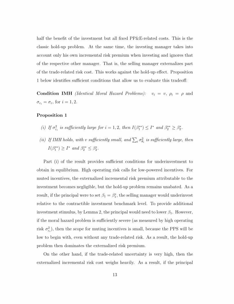
values of F , for which the principal essentially trades off investment and man-
agerial effort distortions. For F above, but close to, F ∗∗(β∗1(1)), the investing
manager’s PPS should be muted, because the investment is sufficiently valuable
to warrant compromises on managerial effort resulting from a reduction in β1.
As fixed costs increase and reach a critical level, denoted F̂ , the principal be-
comes indifferent between inducing the investment—at the expense of reduced
effort incentives for Manager 1—and foregoing it. For F ∈ (F̂ , F ∗] the PPS of
each manager is higher than in the benchmark case. In this region, incomplete
contracting would make it too costly for the principal to induce the investment.
This underinvestment outcome in turn reduces the risk premium.
6
β∗i
-
FF ∗∗(β∗1(1)) F̂ F ∗
I∗ = 1 I∗ = 0
Fig. 2a: Contractible Investment
β∗i (1)
β∗i (0)
6β∗∗1
-
FF ∗∗(β∗1(1)) F̂ F ∗
hhhhhhhhhhhh
I∗∗ = 1 I∗∗ = 0
β∗1(1)
β∗1(0)
6
β∗∗2
-
FF ∗∗(β∗1(1)) F̂ F ∗
I∗∗ = 1 I∗∗ = 0
Fig. 2b: Non-Contractible Investment
β∗2(1)
β∗2(0)
Figure 2: Optimal Contracts and Resulting Investments
Proposition 2 demonstrates that, with severe divisional agency problems, non-
contractibility of investments results in (weakly) higher-powered incentives for
19

the non-investing manager, whereas the effect on the investing manager’s PPS
is ambiguous: higher-powered incentives for relatively high levels of fixed costs
and muted incentives for low values of F .
4.2 Optimal PPS with High Trade-Related Uncertainty(Overinvestment)
As shown in Proposition 1′, when the trade-related uncertainty is high (and ef-
fort is “cheap”), the investment may only be undertaken if it is non contractible
(i.e., if F > F ∗), because the investing manager does not internalize the entire
incremental trade-related risk premium. The principal can mitigate this over-
investment problem by adjusting the investing manager’s PPS. The question,
again, is whether it is optimal to do so. As before, this boils down to a discrete
comparison of the respective values of the two discrete optimization problems:
P∗∗(1) (Allow investment): for any F ∈ [F ∗, F ∗∗(β∗1(0))]:
maxβ
Π(β | I = 1),
subject to β1 ≤ β∗∗1 (F ).
P∗∗(0) (Prevent investment): for any F ∈ [F ∗, F ∗∗(β∗1(0))]:
maxβ
Π(β | I = 0),
subject to β1 > β∗∗1 (F ).
In order to curb Manager 1’s overinvestment tendency (Program P∗∗(0)),
the principal needs to give the investing manager higher-powered incentives:
β∗∗1 = β∗∗1 (F ) + δ, δ → 0.7 Alternatively, the principal can acquiesce to the
overinvestment problem (Program P∗∗(1)) by setting β∗∗i = β∗i (1) for each man-
ager i = 1, 2. As compared with the case of contractible investment, where no
7Note that β∗∗1 (F ) > β∗1(0) for any F < F ∗∗(β∗1(0)).
20

investment would be made, this calls for lower-powered incentives for both agents
because of the additional trade-related risk premium.
The following result characterizes the optimal contract for non-contractible
discrete investments in case of high trade-related uncertainty.
Proposition 3 Suppose the investment choice is binary and non-contractible,
IMH holds with v sufficiently low, and∑
i σ2θi
is sufficiently high, so that F ∗ <
F ∗∗(β∗1(0)).
(i) If F ≥ F ∗∗(β∗1(0)), then β∗∗i = β∗i = β∗i (0), i = 1, 2. Manager 1 does
not invest and non-contractibility does not impose additional costs on the
principal.
(ii) There exists a unique F̂ ∈ [F ∗, F ∗∗(β∗1(0))] such that for any F ∈ [F̂ , F ∗∗(β∗1(0))],
β∗∗1 = β∗∗1 (F ) + ε > β∗1 = β∗1(0) and β∗∗2 = β∗2 = β∗2(0). Manager 1 does not
invest but the principal’s payoff is lower than with contractible investment.
(iii) If F ∈ [F ∗, F̂ ), then β∗∗i = β∗i (1) < β∗i = β∗1(0), i = 1, 2. Manager 1 invests.
The principal’s payoff is lower than with contractible investment.
(iv) If F < F ∗, then β∗∗i = β∗i = β∗i (1), i = 1, 2, and Manager 1 invests. The
principal’s payoff is the same as with contractible investment.
Figure 3 is a close analogue to Figure 2, except now the principal trades off
the optimal amount of excess investment against managerial effort distortions.
Again, for extreme values of fixed costs, incomplete contracting does not affect
the contractual outcome, but it does for intermediate values of F . For F larger
than some critical value F̂ , but less than F ∗∗(β∗1(0)), the investing manager’s
PPS is increased so as to curb his overinvestment tendency. For F ∈ [F ∗, F̂ ), it
is optimal for the principal to let the investment go acquiesce to overinvestment.
21

In summary, when trade-related uncertainty is high and eliciting manage-
rial effort is cheap, incomplete contracting leads to overinvestment and (weakly)
lower-powered incentives for managers without investment opportunities. An
ambiguous result obtains for the manager who can invest: his PPS will be weakly
greater (lower) than in the contractible benchmark setting if the fixed cost is suf-
ficiently high (low) so that in equilibrium the principal wants to curb (acquiesce
to) the manager’s overinvestment tendency.
6
β∗i
-
FF ∗ F̂ F ∗∗(β∗1(0))
I∗ = 1 I∗ = 0
Fig. 3a: Contractible Investment
β∗i (1)
β∗i (0)
6β∗∗1
-
FF ∗ F̂ F ∗∗(β∗1(0))
hhhhhhhhhhhhI∗∗ = 1 I∗∗ = 0
β∗1(1)
β∗1(0)
6
β∗∗2
-
FF ∗ F̂ F ∗∗(β∗1(0))
I∗∗ = 1 I∗∗ = 0
Fig. 3b: Non-Contractible Investment
β∗2(1)
β∗2(0)
Figure 3: Optimal Contracts and Resulting Investments
A key tenet of prior work on incomplete contracting in divisionalized firms is
that equilibrium investment levels are independent of managers’ incentive con-
tracts, absent profit sharing. According to this conventional wisdom, if two
22

divisions operate in comparable operating environments but may have differ-
ent scope to make specific investments, the managers should face similar PPS.
We show that this logic breaks down once trade-related risk is accounted for.
Proposition 2 and 3 demonstrate that the optimal response to ex-ante incentive
problems often is to introduce a wedge between managers’ PPS, i.e., to treat
them differentially. Moreover, these results establish a non-monotonic relation
between the ex-ante profitability of investment opportunities (measures here by
fixed cost) and PPS for managers whose investments can add value to intrafirm
trade (see Figures 2 and 3).
5 Assigning Investment Responsibility
A simplifying assumption in our analysis up to this point was that only one di-
vision had an investment opportunity. We now extend the analysis to bilateral
investments and then employ the model to address an important organizational
design question. Should both divisions be organized as investment centers —
each manager choosing his “own” investment — or should authority for both
up- and downstream investments instead be bundled in the hands of one divi-
sional manager, thereby treating the respective other manager as a profit center
manager to be evaluated based on contribution margin only?
We slightly modify the notation to accommodate bilateral investments. Let
Ii ∈ {0, 1} denote the (discrete) relationship-specific investment undertaken in
Division i = 1, 2, at respective fixed costs of Fi, and I ≡ (I1, I2). For instance,
I2 could describe the demand-enhancing effect of sales promotions downstream.
Normalizing the marginal return of I1 and I2 to unity, each, the divisional relevant
costs and revenues from the transaction generalize those in (1) as follows:
C(q, θ1, I1) = (c− I1 − θ1)q and R(q, θ2, I2) = r(q) + (I2 + θ2)q. (14)
23

The efficient quantity for given investments is q∗(θ, I1, I2) ∈ arg maxq R(q, θ2, I2)−
C(q, θ1, I1). Let M(θ, I) = M(q∗(·), θ, I).
At Date 4, the managers again negotiate over the transaction and split the
attainable contribution margin M(θ, I) equally. In the following, we invoke a
weaker form of our earlier “identical moral hazard problems” condition, now
allowing for operating risks, σεi , to differ across divisions:
Condition IMH′: vi = v and ρi = ρ, for i = 1, 2.
We further modify the manager’s trade-related certainty equivalent to accom-
modate bilateral investments,
f(I | βi) ≡ βiE[M(θ, I)]
2− β2
i
ρ
8V ar(M(θ, I)). (15)
To streamline the exposition, and to highlight the effects of assigning au-
thority across divisions, we make a number of simplifying assumptions. First,
the investments are equally costly, F1 = F2 ≡ F , which, together with (14),
implies that they are equally productive. None of the results to follow hinge
on this restriction. Second, we focus here on the case where both investments
are sufficiently productive such that the principal would choose I∗ = (1, 1) if in-
vestments were contractible. Third, the divisional agency problems are assumed
sufficiently severe so that, as in Section 4.1, the managers tend to underinvest
with incomplete contracting (i.e., the hold-up problem dominates the external-
ized risk premium). We then ask which organizational mode yields the higher
expected surplus for the principal.
With contractible investments, the principal will induce an investment profile
I∗ = (1, 1) if and only if:8
Π∗(1, 1) ≥ max{Π∗(1, 0), Π∗(0, 0)}, (16)
8Given our maintained assumption that investments are of equal productivity, we haveβ∗i (1, 0) ≡ β∗i (0, 1), i = 1, 2, f(1, 0 | β) ≡ f(0, 1 | β), for any β, and Π∗(1, 0) = Π∗(0, 1).
24

where
Π∗(I) ≡ Eθ[M(θ, I)]− (I1 + I2)F
+2∑i=1
[Φi(β
∗i (I))−
ρi8
(β∗i (I))2 · V ar(M(θ, I))
]describes the principal’s expected payoff, with
β∗i (I) ∈ arg maxβi
{Φi(βi)−
ρi8β2i · V ar(M(θ, I))
}as the optimal PPS conditional on a given (contracted) investment profile.
We now return to the setting with non-contractible investments and consider
two organizational modes. Under the “IC-IC ” mode, each division is organized
as an investment center and each manager’s performance is measured on the
basis of profit net of divisional fixed costs (superscript “I” for IC-IC ):
πIi = ai + ε̃i +M(θ, I)
2− FIi, i = 1, 2.
Under the “PC-IC ” mode, one division manager, say, k, is given authority to
choose both I1 and I2. The other manager, l 6= k, is evaluated solely based on
contribution margin. The respective performance measures thus read (super-
script “P” for PC-IC ):
πP ki = ai + ε̃i +
M(θ, I)
2− (I1 + I2)F1ki,
where 1ki ∈ {0, 1} is an indicator that takes the value of 1 if and only if i = k.
In the following, for each organizational mode, we describe how the optimal
PPS and equilibrium investments vary in the ex-ante profitability of investments,
measured by F . We then conduct the the performance comparison.
5.1 Both Divisions are Investment Centers (IC-IC mode)
Consider first the IC-IC mode, i.e., each division chooses (and gets charged for in
its P&L) its own investment. The investment choices must form a (pure-strategy)
25

Nash equilibrium. In prior incomplete-contracting transfer pricing models, di-
visional investments are strategic complements. Ignoring any transfer-related
risk, if by investing more the seller lowers his variable cost, the expected trading
quantity will increase, which in turn raises the marginal return to the buyer’s in-
vestment in revenue enhancement. On the other hand, the trade-related variance
(and thus the risk premium) in (15) also has increasing differences in I1 and I2.
This effect in isolation would make divisional investments strategic substitutes.
To evaluate this tradeoff, denote σε ≡ maxi σεi , σε ≡ mini σεi and the corre-
sponding PPS under contractible investments, respectively, by β∗(I) ≡ mini β∗i (I)
and β̄∗(I) ≡ maxi β∗i (I), for any I. (Given IMH′, the division manager facing
greater operating uncertainty will have the lower PPS.)
Lemma 3 For σεi sufficiently high, the function f(I1, I2 | βi), as defined in (15),
has strictly increasing differences in I1 and I2, for βi = β̄∗i (1, 1).
The proof follows immediately from inspection of (15).9 Lemma 3 relies on
the fact that, for high levels of operating uncertainty, the equilibrium PPS will
be small. The strategic complementarity of the expected contribution margin
then is the dominant force. Lemma 3 readily extends to values of β < β̄∗(1, 1).
Note that in any Nash equilibrium involving I = (1, 1), the optimal PPS’s are
bounded from above by β̄∗(1, 1).
We now turn to the simultaneous move investment game between the man-
agers, for any given PPS βi = β̄ and βj = β ≤ β̄. The investment profile
9As βi in (15) becomes small, the strict supermodularity in I1 and I2 that is inherent in theshared contribution margin dominates the decreasing differences inherent in the risk premiumterm. At the same time, in any Nash equilibrium under the IC-IC mode that supports I = (1, 1)it is never optimal for the principal to set βi > β∗(1, 1) where (given IMH′):
β∗i (1, 1) =1
1 + ρv[σ2εi + V ar(M(θ,1,1))
4
] .Since β∗i (1, 1) is decreasing in σεi , Lemma 3 follows.
26

I = (1, 1) then constitutes a Nash equilibrium, holding fixed the benchmark
PPS, whenever the fixed investment cost is low enough such that
f(1, 1 | β̄)− β̄F ≥ f(0, 1 | β̄). (17)
At the same time, (0, 0) is a Nash equilibrium if F is high enough such that
f(1, 0 | β)− βF ≤ f(0, 0 | β). (18)
Note that (17) is cast in terms of the manager with the higher PPS, β̄, as he
will internalize a greater share of the incremental trade-related risk premium.
Conversely, (18) is cast in terms of the manager with the lower PPS, β, as it is
this manager who is more eager to break away from I = (0, 0).
Games of strategic complementarity are routinely afflicted by multiple equi-
libria, and this is true also for the IC-IC mode. The following result however
shows that, whenever multiple equilibria exist, the desired one that has both
managers investing Pareto-dominates (for the two division managers) the equi-
librium that entails no investments.
Lemma 4 Consider the IC-IC mode under Condition IMH′ with PPS β and
β̄. For β̄ − β sufficiently small, there exist fixed cost parameters, F , for which
I = (1, 1) and I = (0, 0) each are Nash equilibrium investment profiles, but then
(1, 1) is the Pareto-dominant one. For β̄−β large, if (1, 1) is a Nash equilibrium
(i.e., (17) holds), then it is the unique one.
Lemma 4 allows us to disregard the no-investment equilibrium as long as
I = (1, 1) constitutes an equilibrium. It is straightforward then to generalize
Proposition 2 to the bilateral investment case under the IC-IC mode (in the
presence of severe moral hazard). First, given the supermodularity property of
the investment game (by Lemma 3), Lemma 2 carries over directly to bilateral
27

investments: each manager’s investment incentives are decreasing in his PPS,
c.p.. Denote by F I the threshold fixed cost level up to which the benchmark
solution of I = I∗ = (1, 1) can be implemented without having to deviate from
the benchmark PPS (superscript “I ” for IC-IC ):
F I ≡ f(1, 1 | β̄)− f(0, 1 | β̄)
β̄. (19)
Put differently, (17) becomes binding at F I for the manager with the higher PPS.
By Lemma 2, to induce bilateral investments for F > F I , the principal
needs to reduce the higher PPS just enough to make (17) binding. Denote the
resulting PPS by β̄I(F ). By Lemma 2, β̄I(F ) is a decreasing function. At fixed
cost levels for which β̄I(F ) = β∗(1, 1), the principal needs to start also reducing
the lower PPS for the manager who initially faced a lower PPS in lockstep, i.e.,
βI(F ) ≡ β̄I(F ) ≡ βI(F ). At the critical level F̂ I , the PPS distortions required to
ensure I = (1, 1) is an equilibrium investment profile become too costly and the
principal instead induces I = (0, 0) by raising each manager’s PPS to β∗i (0, 0).
6
β∗i
-
FF I F̂ I F ∗
I∗ = (1, 1) I∗ = (0, 0)
Fig. 4a: Contractible Investment
β̄∗(1, 1)
β∗(1, 1)
β̄∗(0, 0)
β∗(0, 0)
6βi
-
FF I F̂ I F ∗
hhhhhhhhhhhh
I∗∗ = (1, 1) I∗∗ = 0
β̄∗(1, 1)
β∗(1, 1)
β̄∗(0, 0)
β∗(0, 0)
Fig. 4b: Non-Contractible Investment
Figure 4: Optimal PPS and Induced Investments Under IC-IC
28

Rather than formally stating a version of Proposition 2 modified for bilateral
investments under the IC-IC mode, we depict the optimal PPS and resulting
investments graphically in Figure 4.
5.2 Concentrating Investment Authority Within One Di-vision (PC-IC mode)
We now turn to the PC-IC mode in which the managers are treated asymmet-
rically: one manager — the “investment center manager” — is given authority
to choose both up- and downstream investments. Before addressing the issue
of optimal incentives, the principal needs to decide which of the two division
managers to grant this authority. Given that the pressing investment distortion
in this section is, by assumption, underinvestment (due to high operating uncer-
tainty), authority should be assigned to the manager whose division has greater
operating uncertainty. By Lemma 2, this manager is more willing to invest be-
cause, all else equal, he faces a lower PPS and is therefore less sensitive to the
incremental trade-related risk premium as a result of investing.
The investment center manager, facing a PPS of β, will choose investments
according to (superscript “P” for PC-IC ):
IP (β | F ) ∈ arg maxI∈{0,1}2
{f(I | β)−
∑i
IiF
}. (20)
By Lemma 3, only I = (0, 0) or I = (1, 1) are candidates for optimality.10 It is
also immediate to see that condition (17), by which (1, 1) was a Nash equilibrium
under the IC-IC mode, is sufficient for the investment center manager under the
10To see that a “mixed” investment profile, (1,0) or (0,1) (they are economically identical inthis setting), can never be optimal under PC-IC, suppose to the contrary that it is. Then:
f(1, 0 | β)− βF ≥ f(0, 0 | β) ⇐⇒ F ≤ [f(1, 0 | β)− f(0, 0 | β)]/β,
f(1, 0 | β)− βF ≥ f(1, 1 | β)− 2βF ⇐⇒ F ≥ [f(1, 1 | β)− f(1, 0 | β)]/β.
By Lemma 3, however, f(1, 1 | β)− f(1, 0 | β) > f(1, 0 | β)− f(0, 0 | β), a contradiction.
29
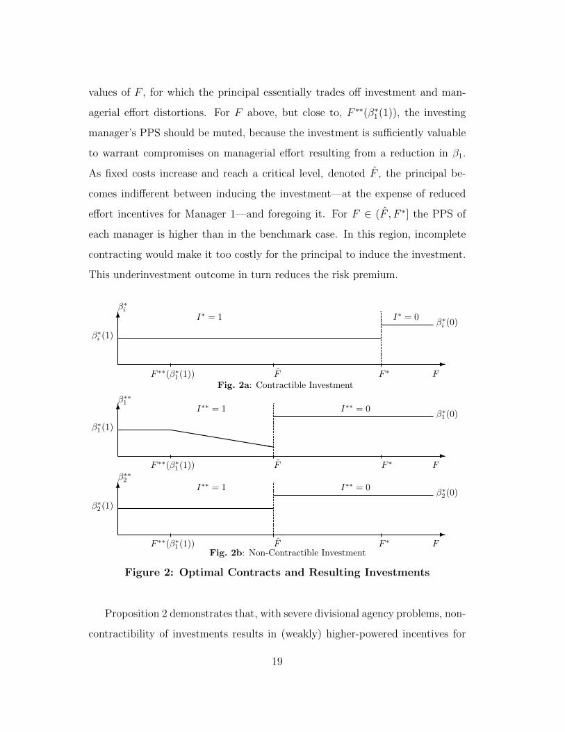
PC-IC to prefer (1, 1) over (1, 0), as he incurs a lower trade-related risk premium.
More generally, the PC-IC mode benefits from the fact that it is the manager
facing lower-powered incentives who makes all investment decisions. On the
other hand, this manager’s P&L now will be charged for the entire fixed costs of∑i IiF , as opposed to only his own divisional fixed cost under IC-IC. This effect,
which we label the “double whammy” effect, exacerbates the hold-up problem.
6
β∗i
-
FFP F̂P F ∗
I∗ = (1, 1) I∗ = (0, 0)
Fig. 5a: Contractible Investment
β̄∗(1, 1)
β∗(1, 1)
β̄∗(0, 0)
β∗(0, 0)
6βi
-
FFP F̂P F ∗
hhhhhhhhh
I∗∗ = (1, 1) I∗∗ = 0
β̄∗(1, 1)
β∗(1, 1)
β̄∗(0, 0)
β∗(0, 0)
Fig. 5b: Non-Contractible Investment
Figure 5: Optimal PPS and Induced Investments Under PC-IC
As in Section 5.1, we describe how investments and PPS vary in F . Since this
is a direct generalization of Proposition 2, we summarize the findings in Figure
5 and omit a formal result. For fixed costs below a threshold F P :
F P ≡f(1, 1 | β)− f(0, 0 | β)
2β, (21)
the contractible benchmark solution is achieved without adjustment to PPS,
i.e., the investment center manager chooses I∗ = (1, 1) facing β∗(1, 1). Again,
generalizing Lemma 2 to the PC-IC mode, shows that to induce investment for
30

F > F P , the principal needs to reduce the investing manager’s PPS. Denote
the resulting PPS by βP (F ). By Lemma 2, βP (F ) is a decreasing function. As
long as I = (1, 1) is induced, the profit center manager’s PPS remains equal to
β̄∗(1, 1). Once fixed costs reach the critical level F̂ P , the distortion in PPS for
the investing manager necessary to induce I = (1, 1) becomes too costly and
the principal is better off foregoing the investment. In that case, each division
manager’s PPS jumps up to βi = β∗i (0, 0), i = 1, 2.
5.3 Comparing the Organizational Modes
We now turn to a performance comparison of the two alternative ways of allocat-
ing investment authority within the firm, IC-IC versus PC-IC. Evaluating the
principal’s expected payoff under these organizational modes, we find:
Proposition 4 Given Condition IMH’, σεi sufficiently large, i = 1, 2, and (16)
holds (i.e., F ≤ F ∗):
(i) For ∆σε ≡ |σεi − σεj | sufficiently small, the principal prefers IC-IC.
(ii) If ∆σε is sufficiently large and R(·) sufficiently concave in q, then the prin-
cipal prefers PC-IC.
The intuition for this result can best be grasped by directly contrasting the
relevant investment incentive constraints under the two modes, holding constant
the PPS. We refer back to two key earlier observations. As argued above, if
I = (1, 1) is a Nash equilibrium under IC-IC, then: (i) the principal can rest
assured the agents will play this equilibrium (even if is not unique); and (ii) the
investment center manager under PC-IC also will prefer I = (1, 1) to investing in
only one of the two divisions. However, because of the double whammy effect, the
investment center manager under PC-IC may actually prefer I = (0, 0). Now,
31

the constraint ensuring (1, 1) is a Nash equilibrium under IC-IC reads
F ≤ f(1, 1 | β̄)− f(1, 0 | β̄)
β̄
≡ F I(β̄), (22)
whereas that ensuring the investment center manager under PC-IC prefers I =
(1, 1) to I = (0, 0):
F ≤f(1, 1 | β)− f(0, 0 | β)
2β
=f(1, 1 | β)− f(1, 0 | β)
2β+f(1, 0 | β)− f(0, 0 | β)
2β
= F P (β). (23)
By strategic complementarity of investments (Lemma 3), F P (β) < F I(β),
for given β. That is, if the managers face (roughly) similar PPS, because their
divisions operate under similar operating risks, then the IC-IC mode generates
stronger investments incentives in aggregate. The reason is that ensuring high
levels of complementary inputs in form of a Nash equilibrium is “cheap” and the
principal need not worry about the undesired (0, 0) equilibrium. In contrast, the
“double whammy” effect under the PC-IC makes the investment center manager
less willing to invest. As we show in the proof, the logic extends beyond a simple
ranking of F I and F P . Hence, if manager face (roughly) similar operating risks,
IC-IC is the preferred mode.
On the other hand, the benefit of concentrating investment authority in the
hand of one division manager is that the principal can take advantage of the
PPS/investments link highlighted above. If ∆σε is high, then by assigning in-
vestment authority to the manager whose division is more volatile (who hence
has a lower PPS, c.p.), the underinvestment problem can be mitigated. If at the
same time the degree of strategic complementarity is limited, then the risk effect
32

will weigh more heavily. An important determinant of the strategic complemen-
tarity between investments is the curvature of the firm’s revenue function, R(·).
The more concave revenues are in q, the smaller is
(f(1, 1 | β)− f(1, 0 | β))−(f(1, 0 | β)− f(0, 0 | β)
),
for any β. Therefore, if the divisions face sufficiently different volatility and,
at the same time, the revenue function for the final product is highly concave,
then the risk effect outweighs the double whammy effect and makes PC-IC the
preferred mode for the principal (part (ii) of Proposition 4).
In sum, the horse race between an “equitable” organizational mode and one
that concentrates all investment decision authority in the hands of one division
is jointly decided by two forces: the relative volatility in the divisions’ operating
environments and the demand (or market) structure in the final product market.
6 Concluding Remarks
This paper has studied how the PPS for divisional managers affects their incen-
tives to invest and engage in intrafirm trade. We find that introducing a wedge
between division managers’ PPS can increase shareholder value. The reason is
that investments in fixed assets add compensation risk by increasing the expected
level of trade. Therefore, muting (increasing) the incentives of the manager who
has an investment opportunity, relative to that of other managers in otherwise
comparable business units, will raise (decrease) his willingness to invest. Hence,
the need to elicit relationship-specific investments to foster intrafirm trade may
introduce a wedge in the PPS of managers of otherwise similar divisions.
The PPS/investment link also has implications for organizational design.
Some business units in practice are designated as profit centers, without invest-
ment authority, others as investment centers with PP&E charges netted against
33

contribution margin. We show that treating divisions asymmetrically — i.e., by
designating one as an investment center in charge of choosing investments for
both divisions engaged in a transaction and the other as a profit center — may
be beneficial, in particular in cases where the divisions face significantly different
operating risks. In that case, the manager facing greater operating risk should
be given investment authority as for him the incremental trade-related risk pre-
mium will be relatively small (because of low-powered incentives). On the other
hand, if the divisions face rather similar operating risks, then it is preferable
to allocate investment authority evenly between the managers, i.e., designating
each division as its own investment center, because that way the overall hold-up
problem is reduced.
34

Appendix
Proof of Lemma 1: Follows from (6) and (7), together with the fact that
V ar(M(θ, I)) is increasing in I. To see that V ar(M(θ, I)) is increasing in I start
by noting that V ar(M(θ, I)) = Eθ[M(θ, I)2] − (Eθ[M(θ, I)])2, by definnition.
Therefore,
∂V ar(M(θ, I))
∂I= Eθ [2M(θ, I) ·MI(θ, I)]− 2Eθ[M(θ, I)] · Eθ [MI(θ, I)]
= 2Cov (M(θ, I),MI(θ, I)) (24)
Applying the Envelope Theorem we note thatMI(θ, I) = Mθ1(θ, I) = Mθ2(θ, I) =
Eθ[q∗(θ, I)] > 0 and further observe that all second and third partial and cross-
partial derivatives ofM(θ, I) are non-negative and conclude thatM(θ, I), MI(θ, I)
and MII(θ, I) are monotonic increasing functions. It follows that for any θo < θoo,
M(θo, I) < M(θoo, I) and MI(θo, I) < MI(θ
oo, I). This in turn demonstrates that
Cov(M(θ, I),MI(θ, I)) > 0 and therefore, ∂V ar(M(θ,I))∂I
> 0. This completes the
proof of Lemma 1.
Proof of Lemma 2: Denoting the (non-effort related part of the) selling
agent’s objective in (9) by π̂1, the necessary first-order condition associated with
(9) reads:
∂π̂1
∂I= β1
(Eθ[q
∗(θ, I)]
2− F ′(I)− ρ1
8β1∂V ar(M(θ, I))
∂I
)= 0. (25)
The second derivative of π̂1 with respect to I at the optimal investment choice
I(β1) and the optimal quantity q∗(θ, I(β1)) is given by:
∂2π̂1
∂I2= β1
(1
2
∂Eθ[q∗(θ, I(β1))]
∂I− F ′′(I(β1))− ρ1
8β1∂2V ar(M(θ, I(β1)))
∂I2
). (26)
Since F (·) is assumed sufficiently convex, to show that (26) is negative we need
to verify that the second derivative with respect to I of the variance of the trade
35

surplus at the optimal quantity is positive. This is indeed true for any I because:
∂2V ar(M(θ, I))
∂I2= 2Eθ [MI(θ, I) ·MI(θ, I)] + 2Eθ [M(θ, I) ·MII(θ, I)]
−2Eθ [MI(θ, I)] · Eθ [MI(θ, I)]− 2Eθ [M(θ, I)] · Eθ [MII(θ, I)]
= 2Cov (M(θ, I),MII(θ, I)) + 2V ar(MI(θ, I)). (27)
To see that ∂2V ar(M(θ,I))∂I2
> 0 note that V ar(MI(θ, I)) > 0, because MIθ(θ, I) > 0
and that Cov(M(θ, I),MII(θ, I)) ≥ 0, because both M(θ, I) and MII(θ, I) are
monotonic increasing functions as shown in the Proof of Lemma 1. It follows
that ∂2π̂1∂I2
< 0
By the Implicit Function Theorem, to show that the optimal investment
choice I(β1) is non-increasing in β1, we need to verify that ∂2π̂1∂I∂β1
≤ 0 at the
optimal investment choice I(β1) and the optimal quantity q∗(θ, I(β1)). That
however follows immediately from (25) because
∂2π̂1
∂I∂β1
=Eθ[q
∗(θ, I(β1))]
2− F ′(I(β1))− ρ1
4β1∂V ar(M(θ, I(β1)))
∂I,
together with β1, ρ1, and ∂V ar(M(θ,I(β1)))∂I
all being positive.
Proof of Proposition 1:
Part (i) If the investment is contractible, the first-order derivative of the
principal’s objective function with respect to investment I∗ is
g∗(I | β∗i ) ≡ Eθ[q∗(θ, I)]− F ′(I)−
∑i ρi(β
∗i )
2
8· ∂V ar(M(θ, I))
∂I. (28)
With non-contractible investments, Manager 1’s marginal benefit from increasing
I equals
g∗∗(I | β1) ≡ f ′(I | β1)− β1F′(I)
= β1
(Eθ[q
∗(θ, I)]
2− F ′(I)− ρ1β1
8· ∂V ar(M(θ, I))
∂I
). (29)
36

A sufficient condition for I∗ ≥ I∗∗(β1) is that the expression in (28) exceeds
that in (29) for any β1. Since β1 ≤ 1,
g∗(I | β∗i )− g∗∗(I | β1) ≥ Eθ[q∗(θ, I)]
2− 1
8· ∂V ar(M(θ, I))
∂I
(∑i
ρi(β∗i )
2 − β1
)
≥ Eθ[q∗(θ, I)]
2− 1
8· ∂V ar(M(θ, I))
∂I
∑i
ρi(β∗i )
2
≥ 0,
for σ2εi
sufficiently high, as then β∗i → 0 while q∗(·) remains bounded away from
zero.
It remains to rank the bonus coefficients for Manger 2. Given that I∗ ≥
I∗∗(β1), for any β1, and that ∂V ar(M(θ,I))∂I
> 0, it is straightforward to see that
β∗∗2 ≥ β∗2 .
Part (ii) A sufficient condition for I∗ ≤ I(β1) is that the expression in (28) is
lower than that in (29) for any β1. Since β1 ≤ 1 and since under IMH assumption,
β∗1 = β∗2 = β∗,
g∗(I | β∗)− g∗∗(I | β1) =
(1− β1
2
)Eθ[q
∗(θ, I)]− (1− β1)F ′(I)
−1
8· ∂V ar(M(θ, I))
∂I
(∑i
ρi(β∗i )
2 − ρ1β21
)
≤ Eθ[q∗(θ, I)]
2− ρ
8· ∂V ar(M(θ, I))
∂I
(2(β∗)2 − 1
).
Next, we use Taylor expansions to express V ar(M(θ, I)) and find
∂V ar(M(θ, I))
∂I≈ 2q∗(µ, I)
∂q∗(µ, I)
∂I
∑i
σ2θi.
Now note that ∂q∗(µ,I)∂I
> 0 and Eθ[q∗(θ, I)] = q∗(µ, I) Hence,
g∗(I | β∗)− g∗∗(I | β1) ≤ Eθ[q∗(·)]
2
[1− ρ
2
∂q∗(·)∂I
∑i
σ2θi
(2(β∗)2 − 1
)](30)
≤ 0,
37

if v sufficiently low and∑
i σ2θi
sufficiently high. To see this note that as v → 0,
β∗ → 1 and g∗(I | β∗) − g∗∗(I | β1) → Eθ[q∗(θ,I)]2
[1− ρ
2∂q∗(µ,I)
∂I
∑i σ
2θi
]≤ 0 for∑
i σ2θi
sufficiently high.
Given that I∗ ≤ I∗∗(β1), for any β1, and that ∂V ar(M(θ,I))∂I
> 0, it is straight-
forward to see that β∗∗2 ≤ β∗2 .
Alternatively:
A necessary condition for (31) to be negative is that 2(β∗)2 − 1 > 0. This is
satisfied when v < v∗(ρ, σε, σθ), where v∗(.) satisfies:
1
(1 + ρv∗(σ2ε + (q∗(µ, I)2)
∑i σ
2θi
))2=
1
2
A sufficient condition for (31) to be negative is that 1−ρ2∂q∗(µ,I)
∂I
∑i σ
2θi
(2(β∗)2 − 1) <
0, which is true for∑
i σ2θi> s∗(ρ, σε, v), where s∗(.) satisfies:
ρ
2
∂q∗(µ, I)
∂Is∗(
2
[1
(1 + ρv(σ2ε + (q∗(µ, I)2)s∗))2
]− 1
)= 1
Note that ∂v∗(.)
∂∑i σ
2θi
< 0 and ∂s∗(.)∂v
> 0.
Proof of Proposition 1′:
Part (i) We need to show that D ≡ F ∗ − F ∗∗(β∗1(1)) > 0.
38

D =∆M
2+∑i
∆Φi
−ρ1
8
[((β∗1(1))2 − β∗1(1)
)· V ar(M(θ, 1))−
((β∗1(0))2 − β∗1(1)
)· V ar(M(θ, 0))
]−ρ2
8
[(β∗2(1))2 · V ar(M(θ, 1))− (β∗2(0))2 · V ar(M(θ, 0))
]>
∆M
2+∑i
∆Φi
−ρ1
8
[((β∗1(1))2 − β∗1(1)
)· V ar(M(θ, 1))−
((β∗1(1))2 − β∗1(1)
)· V ar(M(θ, 0))
]−ρ2
8
[(β∗2(1))2 · V ar(M(θ, 1))− (β∗2(1))2 · V ar(M(θ, 0))
]=
∆M
2+∑i
∆Φi
−ρ1
8
((β∗1(1))2 − β∗1(1)
)[V ar(M(θ, 1))− V ar(M(θ, 0))]
−ρ2
8(β∗2(1))2 [V ar(M(θ, 1))− V ar(M(θ, 0))]
> 0,
for σ2εi
sufficiently high, as then β∗i (I) → 0, I = 0, 1, and ∆Φi → 0 while ∆M
remains bounded away from zero.
Part (ii) We need to show that D ≡ F ∗ − F ∗∗(β∗1(0)) < 0. Using Taylor ex-
pansions to express V ar(M(θ, I)) and the fact that, given IMH, β∗1(I) = β∗2(I) =
39

β∗(I),
D =∆M
2+∑i
∆Φi
−ρ8V ar(M(θ, 1))
[∑i
β∗i (1))2 − β∗1(0)
]
+ρ
8V ar(M(θ, 0))
[∑i
β∗i (0))2 − β∗1(0)
]=
∆M
2+∑i
∆Φi
−ρ8
∑i
σ2θi
[(q∗(µ, 1))2
(2β∗(1))2 − β∗(0)
)]+ρ
8
∑i
σ2θi
[(q∗(µ, 0))2
(2β∗(0))2 − β∗(0)
)]< 0,
if v sufficiently low and∑
i σ2θi
sufficiently high.
To see this note that as v → 0, βi(I)→ 1 and hence, D → ∆M2
+∑
i ∆Φi −ρ8
∑i σ
2θi
[(q∗(µ, 1))2 − (q∗(µ, 0))2] < 0 for σ2θi
sufficiently high. Note also that
∆Φi < 0. This completes the proof of Proposition 1′.
Proof of Proposition 2: Parts (i) and (iv) are obvious, so we only prove
here parts (ii) and (iii). Denote by Ψ∗ the value of program P∗ and by Ψ∗∗(I)
the value of program P∗∗(I), for I ∈ {0, 1} and F (I) = FI. Thus, for any
F ∈ [F ∗∗(β∗1(1)), F ∗]:
Ψ∗(F ) = Π(β∗(1), I = 1 | F )
Ψ∗∗(1)(F ) = Π(β∗∗1 (F ), β∗2(1), I = 1 | F )
Ψ∗∗(0) = Π(β∗(0), I = 0)
Begin by considering fixed cost values F = F ∗∗(β∗1(1)) + ε for ε → 0. Then,
Ψ∗∗(1)(F ) = Ψ∗(F )− δ, δ → 0, because β∗∗1 (F ) is a continuous function of F and
40

Π(β∗∗1 (F ), β∗2(1), I = 1 | F ) is continuous in both β1 and F . That is, the value of
program P∗∗(1) converges to that of the benchmark program P∗ (with contractible
investment) as ε becomes small. At the same time, Ψ∗∗(0) is bounded away
from Ψ∗(F ) for F close to F ∗∗(β∗1(1)). This holds because, by Proposition 1′,
F ∗∗(β∗1(1)) is strictly less than F ∗, together with the observations that at F ∗ we
have Ψ∗∗(0) = Ψ∗(F ) (by definition of F ∗, Π(β∗(1), I = 1 | F ) = Π(β∗(0), I = 0))
and that Ψ∗(F ) is monotonically decreasing in F . Thus, we have shown that for
F ↓ F ∗∗(β∗1(1)), Ψ∗∗(1)(F ) > Ψ∗∗(0), whereas for F ↑ F ∗, Ψ∗∗(1)(F ) < Ψ∗∗(0).
Lastly, since Ψ∗∗(1)(F ) is monotonically decreasing in F whereas Ψ∗∗(0) is
independent of F , it follows that there exists a unique indifference value F̂ at
which Ψ∗∗(1)(F̂ ) = Ψ∗∗(0). This completes the proof of parts (ii) and (iii).
Proof of Proposition 3: The proof follows a logic similar to that of
Proposition 2. Again, we only prove parts (ii) and (iii), because parts (i) and
(iv) are obvious. Denote by Υ∗ the value of program P∗ and by Υ∗∗(I) the value
of program P∗∗(I), for I ∈ {0, 1} and F (I) = FI. For any F ∈ [F ∗, F ∗∗(β∗1(0))]:
Υ∗ = Π(β∗(0), I = 0)
Υ∗∗(0)(F ) = Π(β∗∗1 (F ) + ε, β∗2(0), I = 0)
Υ∗∗(1)(F ) = Π(β∗(1), I = 1 | F )
Consider F = F ∗∗(β∗1(0)) − η for η → 0. Then, Υ∗∗(0)(F ) = Υ∗ − δ, δ → 0,
because β∗∗1 (F ) is continuous in F and Υ∗∗(0)(F ) is continuous in β1. Note that
Υ∗∗(1)(F ) is lower than Υ∗ for F close to F ∗∗(β∗1(0)) and hence, F ↑ F ∗∗(β∗1(0)),
Υ∗∗(1)(F ) < Υ∗∗(0)(F ).
Now note that at F ∗ we have Υ∗∗(1)(F ) = Υ∗, because by definition of
F ∗, Π(β∗(1), I = 1 | F ) = Π(β∗(0), I = 0). However, Υ∗∗(0)(F ) is lower than Υ∗.
To see this note that Π(β, I = 0) is concave and is maximized at β(0). Further,
recal that β1(F ) is decreasing in F and that by Proposition 1′, F ∗∗(β∗1(0)) is
41

strictly higher than F ∗. Hence, β1(0) = β1(F ∗∗) < β1(F ∗). It is now obvious
that for F ↓ F ∗, Υ∗∗(1)(F ) > Υ∗∗(0)(F ). Lastly, there exists a unique indifference
value F̂ at which Υ∗∗(1)(F̂ ) = Υ∗∗(0).
Proof of Lemma 4: Rewriting (17), the investment profile (1,1) is a Nash
equilibrium investment profile whenever F ≤ F11(β̄), where F11(βi) ≡ f(1,1 |βi)−f(1,0 |βi)βi
.
By (18), the no-investment profile (0,0) constitutes a Nash equilibrium whenever
F > F00(β), where F00(βi) ≡ f(1,0 |βi)−f(0,0 |βi)βi
.
Recall that f(I1, I2|β) has increasing differences in (I1, I2), as shown in Lemma
3. Hence, as β̄ and β converge, so will F11(β̄) ≥ F00(β). In this case, for any
F ∈ [F11(β̄), F00(β)), there exist two pure strategy equilibria, (0, 0) and (1, 1).
However, since f(I1,I2 |βi)βi
is decreasing in βi, (F11(β̄) − F00(β)) is decreasing in
(β̄ − β). For (β̄ − β) sufficiently large, F11(β̄) ≤ F00(β) holds, with the conse-
quence that whenever (1, 1) is a Nash equilibrium, it is the unique one.
We now show that if F11(β̄) > F00(β), then (1,1) Pareto dominates (0,0)
for any F ∈ [F00(β), F11(β̄)]. Pareto dominance of (1,1) over (0,0) requires that
f(1, 1 |βi) − βiF ≥ f(0, 0 |βi) for any βi ∈ {β, β̄}. Rearranging, we get for the
division manager with lower-powered incentives, i.e., βi = β:
f(1, 1 |β)− f(0, 0 |β)
β− F =
f(1, 1 |β)− f(1, 0 |β)
β+f(1, 0 |β)− f(0, 0 |β)
β− F
= F11(β) + F00(β)− F
> F11(β̄) + F00(β)− F
> 0, ∀ F ∈ [F00(β), F11(β̄)].
For the manager with higher-powered incentives, i.e., βi = β̄:
f(1, 1 |β̄)− f(0, 0 |β̄)
β̄− F =
f(1, 1 |β̄)− f(1, 0 |β̄)
β̄+f(1, 0 |β̄)− f(0, 0 |β̄)
β̄− F
= F11(β̄) + F00(β̄)− F
> 0, ∀ F ∈ [F00(β), F11(β̄)].
42

Each manager is better off under (1,1) than under (0,0), if both investment
profiles are Nash equilibria. This completes the proof.
Proof of Proposition 4:
Part (i): To show that IC-IC dominates PC-IC we need to verify the fol-
lowing conditions:
1. F P ≤ F I .
2. F̂ P ≤ F̂ I .
3. ΠI(β, I) ≥ ΠP (β, I) for any F ∈ (F I , F̂ P ].
Start with Condition 1. In the limit,
lim∆σε→0
F P = lim∆σε→0
[f(1, 1 | β)− f(0, 0 | β)]
2β
=[f(1, 1 | β̄)− f(0, 0, | β̄)]
2β̄
=[f(1, 1 | β̄)− f(1, 0 | β̄)]
2β̄+
[f(1, 0 | β̄)− f(0, 0 | β̄)]
2β̄
≤ F I , (31)
using (19), (21) and Lemma 3.
Now continue with Condition 2. Note that F̂ P is defined by:
ΠP ((1, 1), β̄∗(1, 1), βP (F )|F̂ P ) = ΠP ((0, 0), β̄∗(0, 0), β∗(0, 0)) (32)
Denote by
Φ̄(β̄) ≡ a(β̄)− V (a(β̄))− ρ
2β̄2σ2
εi
the effort-related payoff to the principal from the division facing lower operating
uncertainty, and define Φ̄(β) correspondingly. We can now simplify (32):
F̂ P = E[M(θ, (1, 1)] + Φ̄(β̄∗(1, 1)) + Φ(βP (F ))
−ρ8
[(β̄∗(1, 1))2 + (βP (F ))2]V ar(M(θ, (1, 1))
−ΠP ((0, 0), β̄∗(0, 0), β∗(0, 0)) (33)
43

Note that F̂ I is defined by:
ΠI((1, 1), β̄I(F ), βI(F )|F̂ I) = ΠI((0, 0), β̄∗(0, 0), β∗(0, 0)). (34)
This, again, can be simplified to:
F̂ I = E[M(θ, (1, 1)] + Φ̄(β̄I(F )) + Φ(βI(F ))
−ρ8
[(β̄I(F ))2 + (βI(F ))2]V ar(M(θ, (1, 1))
−ΠI((0, 0), β̄∗(0, 0), β∗(0, 0)) (35)
Given that:
ΠP ((0, 0), β̄∗(0, 0), β∗(0, 0)) = ΠI((0, 0), β̄∗(0, 0), β∗(0, 0))
= Π∗((0, 0), β̄∗(0, 0), β∗(0, 0)),
to show that F̂ P ≤ F̂ I , we need to verify that
Φ̄(β̄∗(1, 1)) + Φ(βP )− ρ
8[(β̄∗(1, 1))2 + (βP )2]V ar(M(θ, (1, 1)) ≤
Φ̄(β̄I) + Φ(βI)− ρ
8[(β̄I)2 + (βI)2]V ar(M(θ, (1, 1)) (36)
Taking into account the optimal effort choices yields Φ̄(β) = βv− β2
2v− ρ
2β2σ2 and
Φ(β) = βv− β2
2v− ρ
2β2σ2, ∀β. Substituting and simplifying:
[β̄∗(1, 1)− β̄I(F )]
[1
v−(ρσ2
2+
1
2v+ρ
8V ar(M(θ, (1, 1))
)(β̄∗(1, 1) + β̄I(F ))
]+ [βP (F )− βI(F )]
[1
v−(ρσ̄2
2+
1
2v+ρ
8V ar(M(θ, (1, 1))
)(βP (F ) + βI(F ))
]≤ 0 (37)
Now note that:
β̄∗(1, 1) ≥ β̄I(F ) (38)
βI(F ) ≥ βP (F ) (39)
44

The first inequality follows from Lemma 2. For the second inequality, from
Lemma 3:
βP (F ) =[f(1, 1 | β)− f(0, 0 | β)]
2F
=[f(1, 1 | β)− f(1, 0 | β)]
2F+
[f(1, 0 | β)− f(0, 0 | β)]
2F
≤[f(1, 1 | β)− f(1, 0 | β)]
2F+
[f(1, 1 | β)− f(1, 0 | β)]
2F
= βI(F )
From (38) and (39) it follows that β̄∗(1, 1)− β̄I(F ) > 0 and βP (F )− βI(F ) < 0.
Therefore, a sufficient condition for (37) is that:∣∣∣∣∣∣∣1v−[ρσ2
2+ 1
2v+ ρ
8V ar(M(θ, (1, 1))
](β̄∗(1, 1) + β̄I) ≤ 0
1v−[ρσ̄2
2+ 1
2v+ ρ
8V ar(M(θ, (1, 1))
](βP + βI) ≥ 0
(40)
Summing the two inequalities in (40) and rearranging:
∆σ = σ̄2 − σ2 ≤ 2
ρv
[1
βP (F ) + βI(F )− 1
β̄∗(1, 1) + β̄I(F )
](41)
Given (38) and (39) the expression on the RHS is positive. Hence, for sufficiently
small diferential between the divisional operating uncertainties F̂ P ≤ F̂ I .
Now, note that for any F < F P under both regimes, IC-IC and PC-IC,
the investment profile (1, 1) is achieved with the contractible benchmark PPS,
β∗i (1, 1). Hence, the principal’s payoff is equal under both regimes. For any F ∈
[F P , F I ] the principal’s payoff under PC-IC regime is lower than his respective
payoff under IC-IC regime, because under the former regime by Lemma 2 he
needs to reduce the investing manager’s PPS to achieve the investing profile
(1, 1), whereas under the latter regime the same investing profile is still achieved
with the contractible benchmark PPS. For any F ∈ [F̂ P , F̂ I ] it follows by revealed
preference that ΠP (β, I) ≤ ΠI(β, I). For any F > F̂ I under both regimes the
45
principal finds it very costly to induce investment profile (1, 1) and switches to
(0, 0) and gives the division managers the contractible benchmark PPS β∗i (0, 0).
Hence, for F > F̂ I the principal’s payoff is equal under both regimes.
We cannot rank unambiguously F I and F̂ P . However, as long as F̂ P ≤ F I ,
the IC-IC mode is preferred and no further proof rather than Condition 1 and
Condition 2 is needed. If F̂ P > F I , then we need to verify Condition 3. For any
F ∈ [F I , F̂ P ]:
ΠP (β, I) = E[M(θ, (1, 1)]− F + Φ̄(β̄∗(1, 1)) + Φ(βP )
−ρ8
[(β̄∗(1, 1))2 + (βP )2]1))V ar(M(θ, (1, 1)) (42)
ΠI(β, I) = E[M(θ, (1, 1)]− F + Φ̄(β̄I) + Φ(βI)
−ρ8
[(β̄I)2 + (βI)2]V ar(M(θ, (1, 1)) (43)
To show that ΠP (β, I) ≥ ΠI(β, I) we need to verify that:
Φ̄(β̄∗(1, 1)) + Φ(βP )− ρ
8[(β̄∗(1, 1))2 + (βP )2]V ar(M(θ, (1, 1)) ≤
Φ̄(β̄I) + Φ(βI)− ρ
8[(β̄I)2 + (βI)2]V ar(M(θ, (1, 1))
This, however is the same inequality as (36) which, as shown above, holds for
sufficiently small differential between the divisional operating uncertainty. This
completes the proof of Part (i).
Part (ii): Analogically to Part (i) in order to show that PC-IC dominates
IC-IC, we need to verify the following conditions:
1. F P ≥ F I .
2. F̂ P ≥ F̂ I .
3. ΠP (β, I) ≥ ΠI(β, I) for any F ∈ (F I , F̂ I ] .
46

Start with Condition 1. To see that F P ≥ F I note that:
F P ≡f(1, 1 | β)− f(0, 0 | β)
2β
=[f(1, 1 | β)− f(1, 0 | β)]
2β+
[f(1, 0 | β)− f(0, 0 | β)]
2β
>[f(1, 1 | β̄)− f(1, 0 | β̄)]
2β̄+
[f(1, 0 | β̄)− f(0, 0 | β̄)]
2β̄
≈ F I ,
if r(q) is sufficiently concave, so that ∂2
∂I1∂I2f(·) becomes small for any β.
Continue with Condition 2. Analogically to to Part (i) we have to verify
that:
Φ̄(β̄∗(1, 1)) + Φ(βP )− ρ
8[(β̄∗(1, 1))2 + (βP )2]V ar(M(θ, (1, 1)) ≥
Φ̄(β̄I) + Φ(βI)− ρ
8[(β̄I)2 + (βI)2]V ar(M(θ, (1, 1)) (44)
A sufficient condition for (44) to hold is:
∆σ ≤ 2
ρv
[1
βP (F ) + βI(F )− 1
β̄∗(1, 1) + β̄I(F )
](45)
≤ 1
ρv
[1
βP (F )− 1
], (46)
using (38) and (39). Hence, for sufficiently high differential between the general
operating uncertainties Condition 2 holds.
Again, note that for any F < F I the principal’s payoff is equal under both
regimes, because the investment profile (1, 1) is achieved with the contractible
benchmark PPS, β∗i (1, 1). For any F ∈ [F I , F P ] the principal’s payoff under
IC-IC regime is lower than his payoff under PC-IC regime, because under the
former regime by Lemma 2 he needs to reduce the investing manager’s PPS to
achieve the investing profile (1, 1), whereas under the latter regime the same
47

investing profile is still achieved with the contractible benchmark PPS. For any
F ∈ [F̂ I , F̂ P ], ΠP (β, I) ≤ ΠI(β, I) by revealed preference. For any F > F̂ I the
principal’s payoff is equal under both regimes, because he finds it very costly to
induce investment and switches to (0, 0) with the contractible benchmark PPS
β∗i (0, 0).
We cannot rank unambiguously F P and F̂ I . However, as long as F̂ I ≤ F P ,
the PC-IC mode is preferred and no further proof rather than Condition 1 and
Condition 2 is needed. If F̂ I > F P , then we need to verify Condition 3. For any
F ∈ [F P , F̂ I ]:
ΠP (β, I) = E[M(θ, (1, 1)]− F + Φ̄(β̄∗(1, 1)) + Φ(βP )
−ρ8
[(β̄∗(1, 1))2 + (βP )2]1))V ar(M(θ, (1, 1)) (47)
ΠI(β, I) = E[M(θ, (1, 1)]− F + Φ̄(β̄I) + Φ(βI)
−ρ8
[(β̄I)2 + (βI)2]V ar(M(θ, (1, 1)) (48)
To show that ΠP (β, I) ≥ ΠI(β, I) for any F ∈ (F I , F̂ I ] we need to verify that:
Φ̄(β̄∗(1, 1)) + Φ(βP )− ρ
8[(β̄∗(1, 1))2 + (βP )2]V ar(M(θ, (1, 1)) ≥
Φ̄(β̄I) + Φ(βI)− ρ
8[(β̄I)2 + (βI)2]V ar(M(θ, (1, 1))
This, however is the same inequality as (44) which, as shown above, holds for
sufficiently high differential between the divisional operating uncertainty. This
completes the proof.
48

References
[1] Abernethy, M., J. Bouwens and L. van Lent, 2004. Determinants of control
system design in divisionalized firms, The Accounting Review 79(3), 545-570.
[2] Anctil, R. M. and S. Dutta, 1999, Negotiated transfer pricing and divisional
vs. firm-wide performance evaluation, The Accounting Review (January):
87-104.
[3] Baiman, S. and Baldenius, T., 2008, Non-financial performance measures as
coordination devices, Accounting Review, 84(2), 299-330.
[4] Baldenius, T., 2006, Ownership, Incentives and the Holdup Problem, The
RAND Journal of Economics 37(2), 276-299.
[5] Bushman, R., R. Indjejikian, and A. Smith, 1995, Aggregate Performance
Measures in Business Unit Manager Compensation: The Role of Intrafirm
Interdependencies, Journal of Accounting Research 33, 101-128.
Journal of Institutional and Theoretical Economics 146, 85-105.
[6] Holmstrom B. and Tirole, J., 1991, Transfer Pricing and Organizational
Form, Journal of Law, Economics and Organization, 7 (2): 201-228.
[7] Keating, S. 1997, Determinants of divisional performance evaluation in prac-
tice, Journal of Accounting and Economics 24(3), 243-273.
[8] Merchant, K., 1989, Rewarding Results: Motivating Profit Center Managers,
Boston: Harvard Business School Press.
.......... INCOMPLETE ..............
49