A method to detect High Impedance Faults in Distribution ... · High Impedance Faults in...

Sanujit Sahoo

Student Member, IEEE

A method to detect High Impedance Faults in

Distribution Feeders

Mesut Baran

Fellow, IEEE

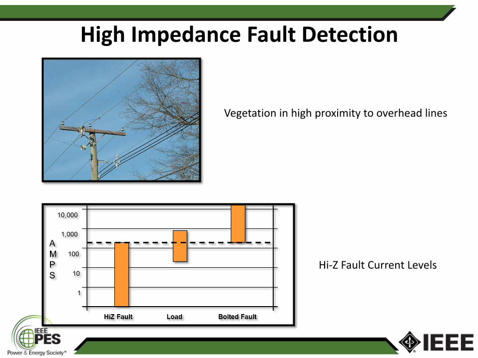
High Impedance Fault Detection

Vegetation in high proximity to overhead lines

Hi-Z Fault Current Levels

Problem Statement

Data from Substation

• Current waveforms

• Voltage waveforms

High Impedance Fault Detection Method

- Possibility of Tree touching overhead lines

Predictive Maintenance by Utility

High Impedance Fault

HIF Detection Method

Data Processing

• Current waveforms obtained at the substation

• Normalization

Feature Extraction

• Decomposition using DWT

• Breaking components into 2 parts each

• Max and Energy of each part

Classification

• Support Vector Machines

Discrete Model for HIF in Simulink

Mayr’s Equation

Continuous version

Discrete version

Step 1: Data Generation & Processing

HIF model had the following components in series: • Arc component (Mayr’s Arc Model) • High Impedance

Challenge: Difficult to obtain current waveforms related to HIFs from utilities

HIF current waveforms

900 1000 1100 1200-20

-10

0

10

20

Fau

lt cu

rren

t(A

)

Time samples

1000 1100 1200 1300-20

-10

0

10

20

Fau

lt cu

rren

t(A

)

Time samples

HIF current waveform in one of the references

HIF current waveform obtained from our model

Step 1: Data Generation & Processing

Step 1: Data Generation & Processing Test Circuit

• HIFs and the other switching events were simulated at different line segments • 55 waveforms for HIF and 129 waveforms for other events were obtained

MRA using Discrete Wavelet Transform

Original Signal

Frequency Range: 0-f Hz

D1

(f/2-f Hz)

A1

(0-f/2 Hz)

D2

(f/4-f/2 Hz)

A2

(0-f/4 Hz)

D3

(f/4-f/8 Hz)

A3

(0-f/8 Hz)

D4

(f/8-f/16 Hz)

A4

(0-f/16 Hz)

Step 2: Feature Extraction


0 100 200 300 400 500 600-2

0

2Original Neutral Current Signal Normalized

0 100 200 300 400 500 600-2

0

2A5(0-60Hz)

0 100 200 300 400 500 600-2

0

2D5(60-120Hz)

0 100 200 300 400 500 600-0.2

0

0.2D4(120-240Hz)

0 100 200 300 400 500 600-0.1

0

0.1D3(240-480Hz)

0 100 200 300 400 500 600-0.05

0

0.05D2(480-960Hz)

0 100 200 300 400 500 600-5

0

5x 10

-3 D1(960-1920Hz)

0 100 200 300 400 500 600-2

0


0 100 200 300 400 500 600-2

0

2A5(0-60Hz)

0 100 200 300 400 500 600-2

0

2D5(60-120Hz)

0 100 200 300 400 500 600-0.2

0

0.2D4(120-240Hz)

0 100 200 300 400 500 600-0.1

0

0.1D3(240-480Hz)

0 100 200 300 400 500 600-0.05

0

0.05D2(480-960Hz)

0 100 200 300 400 500 600-5

0

5x 10

-3 D1(960-1920Hz)

0 100 200 300 400 500 600-2

0


0 100 200 300 400 500 600-2

0

2A5(0-60Hz)

0 100 200 300 400 500 600-2

0

2D5(60-120Hz)

0 100 200 300 400 500 600-0.2

0

0.2D4(120-240Hz)

0 100 200 300 400 500 600-0.1

0

0.1D3(240-480Hz)

0 100 200 300 400 500 600-0.05

0

0.05D2(480-960Hz)

0 100 200 300 400 500 600-5

0

5x 10

-3 D1(960-1920Hz)

Normal HIF HIF

Analysis of waveforms

0 100 200 300 400 500 600-2

0


0 100 200 300 400 500 600-2

0

2A5(0-60Hz)

0 100 200 300 400 500 600-2

0

2D5(60-120Hz)

0 100 200 300 400 500 600-0.2

0

0.2D4(120-240Hz)

0 100 200 300 400 500 600-0.1

0

0.1D3(240-480Hz)

0 100 200 300 400 500 600-0.05

0

0.05D2(480-960Hz)

0 100 200 300 400 500 600-5

0

5x 10

-3 D1(960-1920Hz)

Cap Bank Switching

0 100 200 300 400 500 600-2

0


0 100 200 300 400 500 600-2

0

2A5(0-60Hz)

0 100 200 300 400 500 600-2

0

2D5(60-120Hz)

0 100 200 300 400 500 600-0.5

0

0.5D4(120-240Hz)

0 100 200 300 400 500 600-0.1

0

0.1D3(240-480Hz)

0 100 200 300 400 500 600-0.05

0

0.05D2(480-960Hz)

0 100 200 300 400 500 600

-101

x 10-3 D1(960-1920Hz)

Load Switching

Step 2: Feature Extraction Analysis of waveforms


• Max_D1_Part1: Maximum value of the first part of the D1 component



• Energy_D1_Part1: Energy of the first part of the D1 component



• Max_D1_Part2: Maximum value of the second part of the D1 component



• Energy_D1_Part2: Energy of the second part of the D1 component



Extracted Features

Step 3: Classification

• Constructs a decision surface such that the margin of separation between the two data sets (labeled +1 and -1) is maximized

• In case of non linear data, the original feature space can always be mapped to some higher-dimensional feature space where the training set is separable. The “Kernel Trick” is used

Support Vector Machines

Performance Measures

𝑨𝒄𝒄𝒖𝒓𝒂𝒄𝒚 =# 𝒐𝒇 𝒔𝒂𝒎𝒑𝒍𝒆𝒔 𝒄𝒐𝒓𝒓𝒆𝒄𝒕𝒍𝒚 𝒄𝒍𝒂𝒔𝒔𝒊𝒇𝒊𝒆𝒅

𝒕𝒐𝒕𝒂𝒍 # 𝒐𝒇 𝒔𝒂𝒎𝒑𝒍𝒆𝒔

Actual Positive Class Actual Negative Class

Predicted Positive Class True Positive (TP) False Positive(FP)

Predicted Negative Class False Negative(FN) True Negative(TN)

Confusion Matrix

Step 3: Classification

Parameter selection for SVM

-5 -4 -3 -2 -1 0 10

10

20

30

40

50

60

70

80

90

100

log10

(Gamma value)

Acc

urac

y

log10

(C) = 1

log10

(C) = 2

log10

(C) = 3

log10

(C) = 4

log10

(C) = 5

log10

(C) = 6

log10

(C) = 7

Variation of accuracy of SVM with change in the value of C and gamma

Test Results

Test Results

Average Correct Classification 94.86%

Average Incorrect Classification 5.14%

HIF Non-HIF Classified as HIF 26.81% 2.22% Classified as Non HIF 2.92% 68.05%

Sensitivity (Ratio of HIF classified correctly) 0.9018

Specificity (Ratio of non HIF classified correctly) 0.9684 g-mean 0.9345

Precision of HIF prediction 0.923

5

Precision of non – HIF prediction 0.958

8

Sensitivity Analysis

Test Results

Conclusions

• The performance of the SVM classifier is very good. Since only the neutral current is being used, one classifier can detect HIFs in all three phases making it a cost effective device.

• The data used in this work was obtained from simulations. Although, the modeling of HIF was done accurately, the performance of the classifiers will take a dip once they are trained and tested with real data.

A method to detect High Impedance Faults in Distribution ... · High Impedance Faults in...

Documents

Transcript of A method to detect High Impedance Faults in Distribution ... · High Impedance Faults in...