Page 1. Joe Brusi, A game of numbers. Understanding Directivity Specifications

A Game of Numbers

(Understanding Directivity Specifications)

José (Joe) Brusi, Brusi Acoustical Consulting Loudspeaker directivity is expressed in many different ways on specification sheets and marketing materials provided by loudspeaker manufacturers. Until there is a benchmark for expressing this data, it will continue to be difficult to compare products produced by companies who utilize different methods. This article will define the most commonly used terms and explain the different ways loudspeaker manufacturers’ directivity information is expressed.

How directivity is measured Complete directivity measurements start with the measurement of the sound pressure level (SPL) at all points on a sphere surrounding the speaker system, in other words the speaker is at the center of that sphere and the distance between the speaker and the surface of this sphere would be equal at all points and should be large when compared to the dimensions of the speaker. The set-up for this type of measurement is shown in Figure 1. These measurements are made at all frequencies so we can ascertain the frequency response at any angle. Typically this measurement is accomplished by placing a microphone at a practical distance (usually around 4 meters or 12 feet) and then rotating the loudspeaker to achieve the different angles. Most often this rotation happens around one axis, so two sets of measurements must be made, one for the vertical and one for the horizontal. The most sophisticated systems can rotate around two axes, so that all points of the sphere can be measured in the same run, providing not only vertical and horizontal polar plots (drawing an analogy with the Globe, that would be the equator and two opposite meridians), but all the polars at oblique angles as well. The end result is a set of frequency response curves for each point of the measurement sphere, with resolution anywhere from 1/24th octave to 1 octave, and angular intervals anywhere from 1º to 10º. One these sets can be plotted as a "waterfall" display (Figure 2), where the high resolution data shows the transition from a flat on-axis frequency response (0º) to a response dominated by bass frequencies behind the cabinet (180º).

On axis

off axis

angle

Level in dB

frequency

Figure 1. Setup for directivity measurement

Figure 2. Waterfall display showing a loudspeaker's frequency response

Page 2. Joe Brusi, A game of numbers. Understanding Directivity Specifications

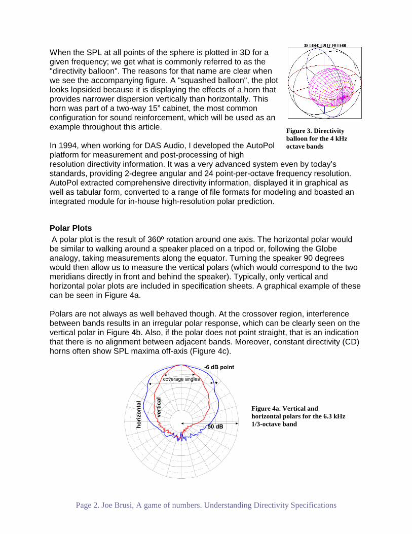
When the SPL at all points of the sphere is plotted in 3D for a given frequency; we get what is commonly referred to as the "directivity balloon". The reasons for that name are clear when we see the accompanying figure. A "squashed balloon", the plot looks lopsided because it is displaying the effects of a horn that provides narrower dispersion vertically than horizontally. This horn was part of a two-way 15” cabinet, the most common configuration for sound reinforcement, which will be used as an example throughout this article. In 1994, when working for DAS Audio, I developed the AutoPol platform for measurement and post-processing of high resolution directivity information. It was a very advanced system even by today’s standards, providing 2-degree angular and 24 point-per-octave frequency resolution. AutoPol extracted comprehensive directivity information, displayed it in graphical as well as tabular form, converted to a range of file formats for modeling and boasted an integrated module for in-house high-resolution polar prediction.

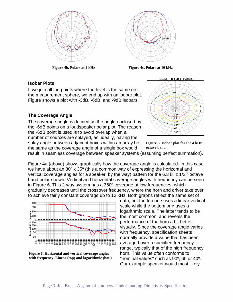
Polar Plots A polar plot is the result of 360º rotation around one axis. The horizontal polar would be similar to walking around a speaker placed on a tripod or, following the Globe analogy, taking measurements along the equator. Turning the speaker 90 degrees would then allow us to measure the vertical polars (which would correspond to the two meridians directly in front and behind the speaker). Typically, only vertical and horizontal polar plots are included in specification sheets. A graphical example of these can be seen in Figure 4a. Polars are not always as well behaved though. At the crossover region, interference between bands results in an irregular polar response, which can be clearly seen on the vertical polar in Figure 4b. Also, if the polar does not point straight, that is an indication that there is no alignment between adjacent bands. Moreover, constant directivity (CD) horns often show SPL maxima off-axis (Figure 4c).

Figure 3. Directivity balloon for the 4 kHz octave bands

Figure 4a. Vertical and horizontal polars for the 6.3 kHz 1/3-octave band

Page 3. Joe Brusi, A game of numbers. Understanding Directivity Specifications

Isobar Plots If we join all the points where the level is the same on the measurement sphere, we end up with an isobar plot. Figure shows a plot with -3dB, -6dB, and -9dB isobars.

The Coverage Angle The coverage angle is defined as the angle enclosed by the -6dB points on a loudspeaker polar plot. The reason the -6dB point is used is to avoid overlap when a number of sources are splayed, as, ideally, having the splay angle between adjacent boxes within an array be the same as the coverage angle of a single box would result in seamless coverage between speaker systems (assuming perfect summation). Figure 4a (above) shows graphically how the coverage angle is calculated. In this case we have about an 80º x 35º (this a common way of expressing the horizontal and vertical coverage angles for a speaker, by the way) pattern for the 6.3 kHz 1/3rd octave band polar shown. Vertical and horizontal coverage angles with frequency can be seen in Figure 6. This 2-way system has a 360º coverage at low frequencies, which gradually decreases until the crossover frequency, where the horn and driver take over to achieve fairly constant coverage up to 12 kHz. Both graphs reflect the same set of

data, but the top one uses a linear vertical scale while the bottom one uses a logarithmic scale. The latter tends to be the most common, and reveals the performance of the horn a bit better visually. Since the coverage angle varies with frequency, specification sheets normally provide a value that has been averaged over a specified frequency range, typically that of the high frequency horn. This value often conforms to "nominal values" such as 90º, 60 or 40º. Our example speaker would most likely

Figure 5. Isobar plot for the 4 kHz octave band

beam

wid

th in

deg

rees

400

400

100

100

50

200

200

300

20

0

2520 31 40 50 63 80 100

125

160

200

250

315

400

500

630

800

1k0

1k25 1k6 2k 2k5

3k15 4k 5k 6k3 8k 10k

12k5 16k

20k

Figure 6. Horizontal and vertical coverage angles with frequency. Linear (top) and logarithmic (bot.)

Figure 4b. Polars at 2 kHz Figure 4c. Polars at 10 kHz

Page 4. Joe Brusi, A game of numbers. Understanding Directivity Specifications

be rated as a 90º X 60º (horizontal x vertical) system.

The Q Factor This is a mathematical expression of how directive a source is. Larger Q factor values denote more directional sources. The Q factor is calculated by comparing the on-axis level with the average level for all the points in the measurement sphere. In practice, Q is often derived from the horizontal and vertical polar plots. A spherical source (a source that has the same output level at all angles, close to a subwoofer at low frequencies) has a Q factor of 1. A hemispherical source, akin to a spherical one that is placed against a wall (this condition is referred to as 2 pi or half space), has a Q of 2. As with coverage angle, different evaluation methods are used which can result in slightly different Q results.

The directivity index (DI) DI is the same as Q factor, but expressed in a logarithmic fashion as follows: DI (in dB) = 10*log (Q) Thus, a spherical source has a Q factor of 1 and a directivity factor of 0 dB, and a hemispherical (half-sphere) source has a Q factor of 2 and a directivity factor of 3 dB. Typical directivity indexes for a horn would spread from 10 to 20 dB, corresponding to Q factors of 10 to 100. The DI for the polars represented in Figure 4 is 12 dB (Q factor of 16). On-axis sensitivity and DI have a direct correlation. For a compression driver/horn from our 2-way speaker example, an X dB more directional horn will result in X dB more sensitivity. Using a subwoofer as an example, when it is placed against a wall it will increase in sensitivity by 3 dB (DI will change from 0 to 3 dB, Q factor from 1 to 2) as compared to its free-field sensitivity. Figure 7 show the DI and Q with frequency for our example 2-way system. We can see a rising response from the 15” woofer, which corresponds to the narrowing of the cone's directivity, as frequency increases (also referred to as “beaming”). In contrast, the directivity that the horn exhibits is fairly constant with frequency, commonly referred to as a CD (constant directivity) horn. DI (Q) and coverage angles are typically plotted for 1/3rd-octave bands.

Q10

100

DI i

n dB

10

15

20

5

0 1

2520 31 40 50 63 80 100

125

160

200

250

315

400

500

630

800

1k0

1k25 1k

6 2k 2k5

3k15 4k 5k 6k

3 8k 10k

12k5 16

k20

k

Figure 7. Q and DI with frequency

There is some disagreement among specification writers as to what the 0-dB reference in the calculation of the coverage angle should be. Some manufacturers take the on-axis level, while some others use the maximum output level exhibited by the polar. If the polar is nice and smooth both criteria will yield the same result, but if they are irregular, such as those in Figures 4b and 4c, resulting coverage angle values may differ significantly.

Page 5. Joe Brusi, A game of numbers. Understanding Directivity Specifications

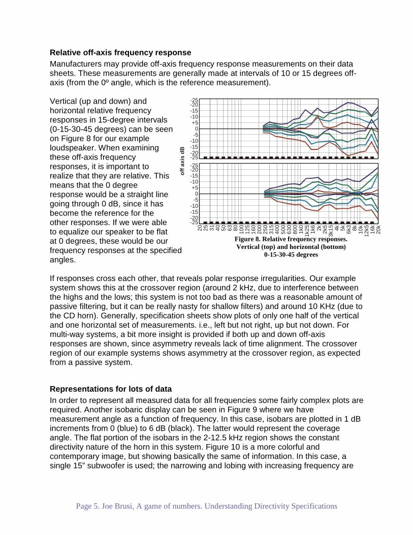
Relative off-axis frequency response Manufacturers may provide off-axis frequency response measurements on their data sheets. These measurements are generally made at intervals of 10 or 15 degrees off-axis (from the 0º angle, which is the reference measurement). Vertical (up and down) and horizontal relative frequency responses in 15-degree intervals (0-15-30-45 degrees) can be seen on Figure 8 for our example loudspeaker. When examining these off-axis frequency responses, it is important to realize that they are relative. This means that the 0 degree response would be a straight line going through 0 dB, since it has become the reference for the other responses. If we were able to equalize our speaker to be flat at 0 degrees, these would be our frequency responses at the specified angles. If responses cross each other, that reveals polar response irregularities. Our example system shows this at the crossover region (around 2 kHz, due to interference between the highs and the lows; this system is not too bad as there was a reasonable amount of passive filtering, but it can be really nasty for shallow filters) and around 10 KHz (due to the CD horn). Generally, specification sheets show plots of only one half of the vertical and one horizontal set of measurements. i.e., left but not right, up but not down. For multi-way systems, a bit more insight is provided if both up and down off-axis responses are shown, since asymmetry reveals lack of time alignment. The crossover region of our example systems shows asymmetry at the crossover region, as expected from a passive system.

Representations for lots of data In order to represent all measured data for all frequencies some fairly complex plots are required. Another isobaric display can be seen in Figure 9 where we have measurement angle as a function of frequency. In this case, isobars are plotted in 1 dB increments from 0 (blue) to 6 dB (black). The latter would represent the coverage angle. The flat portion of the isobars in the 2-12.5 kHz region shows the constant directivity nature of the horn in this system. Figure 10 is a more colorful and contemporary image, but showing basically the same of information. In this case, a single 15” subwoofer is used; the narrowing and lobing with increasing frequency are

Figure 8. Relative frequency responses. Vertical (top) and horizontal (bottom)

0-15-30-45 degrees

1k25

3k15

12k52520 31 40 50 63 80 100

125

160

200

250

315

400

500

630

800

1k0

1k6 2k 2k5 4k 5k 6k3 8k 10k

16k

20k

0+5

-10-15

-5

-20

-10-15

-25

-20-25

0+5

-10-15

-5

-20

-10-15

-25

-20-25

off

axi

s d

B

Page 6. Joe Brusi, A game of numbers. Understanding Directivity Specifications

shown (a bit like a “line array”, except that a correctly design isophasic waveguide should not show any side lobes).

Modeling Electro-acoustic modeling software can be used to display directivity information quite effectively through images that look like weather maps , and visually show how even coverage is throughout the listening area. In the past, these programs utilized fairly crude directivity balloons, typically with 10 degree resolution in octave bands. For the last 10 years the AES (Audio Engineering Society) has been trying to produce a standard for high resolution directivity data to be used by modeling software, but so far not much has been achieved. The CLF universal format (with a maximum 5-degree angular and 1/3rd band resolution) has been adopted by CATT, Ulysses and LARA software. Data resolution on EASE (the de-facto standard), originally 10-degree and 1-octave band, became 5-degree and 1/3rd octave on version 3, and version 4 introduced a format whereby an arbitrary resolution can be used. Modeling software is used by designers to ensure all areas are covered. It is often required by customers when spec’ing a system and it also provides graphically attractive presentation material. The most elaborate programs will be able to show fairly realistic looking rooms in 3D, which, aside from the visual impact side of things, will help customers understand the proposed concept, as they will be able to see the location of the speakers within the room. The projection of the loudspeaker’s directivity onto a coverage area can be seen for EASE and CADP2 (a wonderful but defunct piece of software, made by JBL, that did not make it to the XXI century) in Figures 11 and 12 respectively. A color scale can be seen of the right hand side of each of the images.

Figure 9b. Isobar display from 0 to -10 dB in 1 dB intervals

Figure 9a. Isobar display from 0 to -6 dB in 1 dB intervals

90

angl

e in

deg

rees

03060

-90

-30-60

90

angl

e in

deg

rees

03060

-90

-30-60

2520 31 40 50 63 80 100

125

160

200

250

315

400

500

630

800

1k0

1k25 1k

6 2k 2k5

3k15 4k 5k 6k

3 8k 10k

12k5 16k

20k

Page 7. Joe Brusi, A game of numbers. Understanding Directivity Specifications

About the author: Brusi is a graduate in engineering acoustics from the Institute of Sound and Vibration Research, University of Southampton (UK). He has held positions for professional speaker manufacturers such as JBL Professional (USA) and DAS Audio (Spain). He currently leads his own consulting firm, Brusi Acoustical Consulting.

The original article was published by Sound and Video Contractor magazine (USA) in April 1999. This version was updated in January 2010

Figure 12. Loudspeaker directivity information as shown through CADP2’s area projection

Figure 11. Loudspeaker directivity information as shown EASE's area projection