A finite element study of shell and solid element performance in …808638/FULLTEXT01.pdf · A...

BACHELOR’S THESIS Mechanical Engineering, Product development Department of Engineering Science

March 27, 2015

A finite element study of shell and solid element performance in crash-box simulations Mahdi Bari

BACHELOR’S THESIS

i

Abstract

This thesis comprehends a series of nonlinear numerical studies with the finite element

software’s LS-Dyna and Impetus AFEA. The main focus lies on a comparative crash analysis

of an aluminium beam profile which the company Sapa technology has used during their

crash analysis.

The aluminium profile has the characteristic of having different thickness over span ratios

within the profile. This characteristic provided the opportunity to conduct a performance

investigation of shell and solid elements with finite element analysis.

Numerical comparisons were made between shell and solid elements where measurable

parameters such as internal energy, simulation times, buckling patterns and material failures

were compared to physical tests conducted prior to this thesis by Sapa technology.

The performance investigation of shell and solid elements was initiated by creating models

of the aluminium profile for general visualization and to facilitate the meshing of surfaces.

The meshing procedure was considered to be an important factor of the analysis. The mesh

quality and element orientations were carefully monitored in order to achieve acceptable

results when the models were compared to physical tests.

Preliminary simulations were further conducted in order to obtain a clear understanding of

software parameters when performing crash simulations in LS-Dyna and Impetus AFEA.

The investigated parameters were element formulations and material models. A general

parameter understanding facilitated in the selection of parameters for actual simulations,

where material failure and damage models were used.

In conclusion, LS-Dyna was observed to provide a bigger internal energy absorption during

the crushing of the beam with longer simulation times for solid elements when compared to

shell elements. Impetus AFEA did on the other hand provide results close to physical test

data with acceptable simulation times when compared to physical tests.

The result difference obtained from the FE-software’s in relation to physical crash

experiments were considered to be varied but did indicate that shell elements were efficient

enough for the specific profile during simulations with LS-Dyna. Impetus AFEA proved that

the same time to be numerically efficient for energy approximations with solid elements

refined with the third polynomial.

Date: March 27, 2015 Author: Mahdi Bari Examiner: Thomas Carlberger Advisor: Mats Larsson, University West, Björn Olsson, Sapa Technology Programme: Mechanical Engineering, Product development Main field of study: Mechanical Engineering Education level: first cycle Credits: 15 HE credits Keywords Crash analysis, solid elements, shell elements, LS-Dyna, Impetus AFEA,

Hypermesh Publisher: University West, Department of Engineering Science,

S-461 86 Trollhättan, SWEDEN Phone: + 46 520 22 30 00 Fax: + 46 520 22 32 99 Web: www.hv.se

A finite element study of shell and solid element performance in crash-box simulations

ii

Preface

This thesis was made with great help from the supervisor Mats Larsson at University West.

It is also important to acknowledge Sapa technology for inviting me to discuss the thesis in

person and showing me the facility where some of the tests mentioned in this thesis were

performed.

Finally, I would like to thank the Company supervisor Björn Olsson for providing guidance

throughout the thesis work.


iii

Contents

Abstract ............................................................................................................................................... i

Preface ................................................................................................................................................ ii

Symbols and glossary ........................................................................................................................ v

1 Introduction ................................................................................................................................ 1 1.1 Company description....................................................................................................... 1 1.2 Problem background ....................................................................................................... 2

2 Overview of previous work ...................................................................................................... 2 2.1 Aim and limitations.......................................................................................................... 3

3 Methodology ............................................................................................................................... 3 3.1 External search ................................................................................................................. 4 3.2 Design and simulations ................................................................................................... 4 3.3 Comparison of data ......................................................................................................... 4

4 Theory .......................................................................................................................................... 5 4.1 Crash analysis .................................................................................................................... 5 4.2 Element theory ................................................................................................................. 6

5 Profile design .............................................................................................................................. 8 5.1 Basic design ....................................................................................................................... 8 5.2 Meshing ........................................................................................................................... 10

6 Simulations ................................................................................................................................ 11 6.1 Preparatory simulations ................................................................................................. 11

6.1.1 Element formulation ........................................................................................ 13 6.1.2 Simulation efficiency ........................................................................................ 16

6.2 Choice of parameters ..................................................................................................... 18 6.3 Simulations with shell elements ................................................................................... 19 6.4 Simulations with solid elements ................................................................................... 22

7 Simulations with Impetus AFEA ........................................................................................... 23

8 Further measurements ............................................................................................................. 25

9 Results ........................................................................................................................................ 27

10 Analysis and discussion ........................................................................................................... 28

11 Conclusions and future work ................................................................................................. 29

References ........................................................................................................................................ 30


iv

Appendices

A. Sapa beam

B. Timestep equations

C. Shell and solid CAD models

D. Mesh differences

E. Initial buckling and folding observation

F. Time steps calculated by LS-Dyna

G. Material data

H. Material failure and GISSMO (Visual, Times and Debris)

I. Mesh differences in Impetus AFEA

J. Energy measurements of material failure for shell and solid elements in relation to physical tests

K. Energy comparisons for Impetus AFEA and physical tests

L. Final data comparisons


v

Symbols and glossary

CAD – Computer Aided Engineering

Mesh – Grid of nodes and elements

FEA/FEM- Finite Element Analysis/Method

GISSMO – Generalized Incremental Stress State dependent damage Model

NIP – Number of Integration Points

CPU – Central processing unit

GPU- Graphics processing unit

NDA- Non-disclosure agreement


1

1 Introduction

Understanding how material failure is simulated in a reliable way is considered to be

crucial for the advancing technology in the automotive industry. To be able to safely

predict deformation in a crash analysis, an understanding of how different parameters

such as element formulation and its implications on simulation results is needed.

The analysis was performed on a crash box where the main purpose of the part is to

prevent the adjacent car structure from absorbing even minimal amounts of damage

during low velocity crashes. To be able to measure the amount of damage that the car

structure absorbs, the crash box is analysed by measuring the amount of energy that

can be absorbed by the part.

The choice of whether to use shell or solid elements is often experience based even

though there are some guidelines. Using wrong element types can produce non-

acceptable results [1].

One main inquiry to be investigated is the question whether solid elements produce

more accurate results in relation to shell elements with acceptable simulation times. The

results are implied as the absorbed internal energy during a crash. The main finite

element software which is used during this study is LS-Dyna. A minor comparative

study was also made with the FE-software Impetus AFEA.

This inquiry was based on the fact that the geometry of the crash box is a thin walled

structure with a varying body thickness. The varying body thickness provides different

thickness to span ratios which are to be considered, see Appendix A.

Results from this thesis will provide with an overview of simulation results in LS-Dyna

and Impetus AFEA in relation to physical tests.

1.1 Company description

Sapa Group is the world leader in aluminium solutions with worldwide manufacturing

and distribution of aluminium profiles. Sapa group currently has 23,000 employees in

more than 40 countries with the headquarters located in Oslo, Norway.

Sapa Technology is Sapa’s internal research and development resource located in

Finspång, Sweden. Sapa Technology takes an active part in business development and

technical development of products and processes throughout the group. Sapa

technology conducts development projects in collaboration with Sapa companies and

their customers as well as universities and research institutes [2]. This thesis is made in

collaboration with Sapa Technology and is performed at University West in Trollhättan,

Sweden.


2

1.2 Problem background

Simulations have been performed by Sapa Technology in which the FE-software LS-

Dyna was used. The simulated beam profile consisted of shell elements and was

simulated with different material models. Simulation results showed some concern

regarding deformation when compared to physical tests with the use of shell elements

[2].

Result comparisons with shell and solid elements were requested since a varying

thickness exists within the profile. The purpose was to investigate if more accurate

results could be achieved. Sapa Technology has been using the FE-software Impetus

AFEA for other simulations and has for further comparison requested a result

comparison between the two FE-software’s.

2 Overview of previous work

During previously performed crash tests by Sapa technology, a material model

comparison in LS-Dyna was conducted in order to see which model presents the most

reliable results. Indoor crush tests were performed and compared to simulated data in

order to measure result discrepancy in absorbed energy. The analyzed geometry was a

company specific aluminum profile, see Appendix 11.A.

Following material models were compared:

Isotropic linear plasticity material model without a material failure criteria

Anisotropic material model with material failure criteria named Generalized

Incremental Stress State dependent damage Model (GISSMO).

Company specific material model developed by Simlab in Norway with a failure

criteria and a hardening rule optimized after necking.

The GISSMO model showed the most realistic results in the crush tests due to same

crack behaviours in the simulations as in the indoor tests, see Figure 1.

Figure 1, Indoor crush test and simulation with the GISSMO material model


3

Sapa Technology has also performed an FE-analysis of a three point bending test where

GISSMO showed a slightly more accurate behaviour compared to the other material

models by having a more realistic force-displacement ratio.

Physical crush-tests did in some cases result in a statistical anomaly where the middle-

wall ruptured. This phenomenon was considered to be stochastic.

The conclusion of the performed tests was that the commercial material model

GISSMO is recommended for future simulations over the non-commercial Simlab

model since it is faster and maintains reliable simulation results [2].

2.1 Aim and limitations

The aim of this thesis is to answer the question whether shell elements are good enough

for the crash analysis performed by the company. Conducting a numerical analysis with

solid elements and comparing simulation results with previous work can produce a

general understanding regarding the choice of element type. The numerical study can

further explain if and why one certain type of element produces more reliable results

than the other.

The analysis will solely be focused on crush simulations. The simulation results will be

compared to previous work done by Sapa Technology. The analysis will not include any

physical crush tests since they have already been performed by Sapa Technology.

Simulations will be performed in the FE-software’s LS-Dyna and Impetus AFEA.

3 Methodology

The chosen approach to achieve a progressive yet measurable result span during the

thesis work is divided into three subcategories; Internal and external search, design &

simulations and result comparison. An iterative strategy was used to maintain a good

overview of results achieved in each step, see Figure 2.

Figure 2, Methodology overview

Each of the above mentioned subcategories were executed in a sequence and were not

to be executed in a random order due to the risk of time loss. As seen in Figure 2, an

iterative procedure is combined with the task sequence. The purpose of such procedure

was to maintain an effective work progress.


4

It has been noted by previous experience that it is important to take a step back and

compare the results with already conducted research. In most cases, additional research

is required since surprising anomalies might occur, often caused by initial software

parameters.

Comparing achieved results with company data is the final step in the sequence and

requires thorough understanding of previous steps in order to draw adequate

conclusions.

3.1 External search

Relative information gathered in the courses HFC400 and FMB300 [5, 6] were used as

a starting point when creating a theory basis for the project. Information such as

material data and previous research was provided by Sapa Technology and was used

throughout the thesis work.

The search step was to be continuous throughout the project work. Time efficiency was

considered to be an important factor during the work, hence the search scope was

constrained and adapted by each planned activity. The information search did expand

for each proceeding step in the methodology sequence presented in Figure 2.

3.2 Design and simulations

The computer aided engineering software Siemens PLM NX was used to design

necessary simulation profiles. A finite element pre-processor, in this case Hypermesh

was further used to create different mesh combinations on the designed surfaces.

Simulations with LS-Dyna were executed through an external calculation cluster located

at PTC, Production Technology Centre in Trollhättan, Sweden. Simulations in Impetus

AFEA were executed by the use of the graphical processing unit residing within the

computer. All simulations with LS-Dyna were performed by the use of 12 CPU’s in the

calculation cluster.

3.3 Comparison of data

Comparisons of company data in relation to simulated data were executed in order to

validate performed simulations in a reliable way. Company data contained simulation

results as well as physical test results. Provided data from the company was considered

to be reference information during the thesis work.

The reference information was used as a discrepancy measurement tool when

measuring variations in unit magnitudes obtained from different simulations. The

comparisons were made on the absorbed internal energy and simulation time values

obtained from simulations with shell or solid elements.


5

4 Theory

Performing nonlinear numerical analysis requires a good knowledge basis before the

actual work. This section covers fundamental theory required to perform the analysis.

Covered topics describe important factors of a crash analysis and the importance of

having a good mesh.

4.1 Crash analysis

In order to achieve as reliable numerical results as possible, a good approach is needed.

One of the more distinctive characteristics of a crash is that the events happen during

a short period of time which opens up the possibility of using an explicit numerical

method. Another possibility is to use an implicit approach which is more hardware

demanding since more variables are added in the calculation [7].

Crash analysis is very contact dependent since the ability to simulate an actual crash

relies on multiple factors and can have fatal results if not done correctly [4]. The contact

definition has two main categories to choose from, nodal based contact and segment

based contact. These are further divided into sub categories consisting of one way

respectively two way contact types.

Using a nodal based contact requires more work if different mesh constellations are to

be used since the node identification numbers change depending on the mesh

constellation. Another disadvantage is that the contact search locates the closest nodes

on different segments, which makes this contact definition unstable for meshes

consisting of elements with varying aspect ratios.

The segment based contact searches for node segments during contact which is

preferred during crash analysis. The choice of one way or two way definition lies in

whether both the slave and master part are checked for penetration or if only the slave

part is checked.

To ensure that no penetration occurs before the intended contact, an offset of colliding

parts is recommended, see Figure 3.

Figure 3, Offset for contacts

The offset is recommended to be at least the sum of thickness divided by two [8].


6

4.2 Element theory

The choice of element type is in most cases dependent on the geometry which is to be

analysed. The analysis is being made on a thin walled structure, which provides two

different possibilities to approach the problem. The approaches are whether to use shell

or solid elements. General guidelines mention the length over thickness ratio as a good

reference point where the ratio presents a boundary between the choice of shell and

solid elements [1].

Working with shell and solid elements yields in many different element types to choose

from [10]. The efficiency of an element type is dependent on the surface geometry and

application. In crash analysis, folding or buckling of elements often occur so the chosen

element type must be suitable in definition to withstand and take advantage of such

conditions.

For shell elements, a quadrilateral element type with sufficient amount of integration

points in the element and through the thickness is considered to be efficient when

simulating a crash. The same formulation of integration points is suited for solid brick

elements. Choosing the amount of integration points in an element is considered to be

part the element formulation [11].

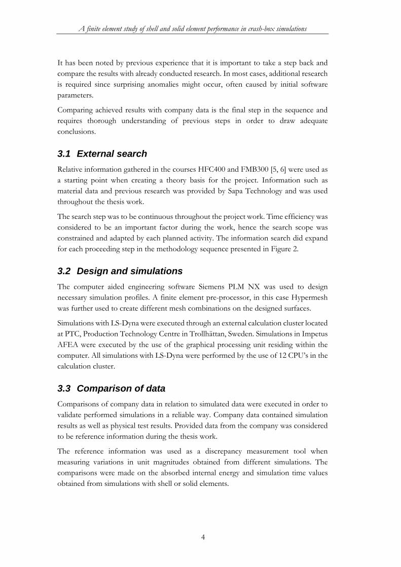
There are some well used element formulations in LS-Dyna when simulations are

performed with quadrilateral shell elements. One of the recommended formulations is

the Belytschko-Lin-Tsay formulation, denoted as “ELFORM=2” which provides one

integration point on the element surface. Another element formulation is the fully

integrated shell formulation, denoted as “ELFORM=16” which provides four

integration points on the element surface, see Figure 4.

Figure 4, Element formulations for quadrilateral shell elements

The amount of integration points on the surface can provide different results in a crash

simulation. Four integration points on the element surface do in most cases provide a

more accurate surface buckling during crash simulations when compared to the one

integration point formulation. More integration points on an element surface can

however facilitate in warping of the element, so hourglass stiffness must be considered

[10].


7

For solid elements, the corresponding element formulations exist with more options if

shear locking is for example present. If eight-noded brick elements are to be used, the

recommended element formulations are either the default formulation with one

integration point, denoted as “ELFORM=1” or the fully integrated solid formulation,

denoted as “ELFORM=2” which provides eight integration points on the element

surface, see Figure 5. [10]

Figure 5, Element formulations for solid brick elements

The described element formulations for shell and solid elements are considered to be

analogous due to the same integration point formulation of the element surface.

The number of integration points (NIP) through the thickness is an important variable.

To achieve a good approximation of the material behaviour during nonlinear

deformation, a higher amount of integration points is recommended. It is important to

note that a higher number of NIP’s results in a longer simulation time but yields

theoretically more correct results. During a crash analysis it is common to have at least

five integration points [11].

Element formulations are further dependent on the element construction where the

element’s skewness, warping and angular deviation are defined with respect to

recommended values. Creating a mesh with poor elements can yield in undesired

simulation results [9].

Another part of the element formulation is the definition of the element’s orientation.

This is done by firstly defining the element orientation with respect to the global

coordinate system. By doing so, a normal vector of an element is defined. The purpose

of defining the element normal lies in keeping track of the NIP’s and simply to keep

track of which side is top or bottom, left or right [11].


8

5 Profile design

Visualizing the beam from different aspects was considered to be an efficient starting

point. Different methods were used to design the profile where the main purpose was

to achieve a model design with different design options for the meshing procedure.

5.1 Basic design

The basic design was constructed by an assembly of two sheet bodies for simulations

with shell elements. For simulations with solid elements, a full thickness body was

made, see Appendix C.

All dimensions were provided by Sapa technology, see Appendix 11.A. The dimensions

were adapted to post performed physical tests, where the crash impact was in the need

of being controlled, hence the angles. The geometry was slightly modified by changing

the starting location of the angles to the starting point of the middle wall radius instead

of the centre of the beam, see Figure 6.

Figure 6, Modified geometry

To create a good base model for the meshing step, some preparations of the designed

model were made. It was desired to have as many quadrilateral elements as possible for

the shell mesh, and brick elements for the solid element mesh. Applied angles in the

beam model were considered to possibly create an uneven distribution of elements in

the meshing process. In order to obtain a homogenous mesh throughout the model,

boundary constrains were needed to be defined in case of mesh editing.


9

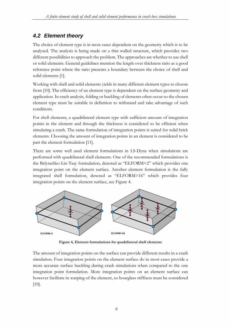
It was known that the crushing of the beam had a fixed distance, so creating equal

lengths on the geometry would push the uneven distribution of elements further to the

bottom where no crushing is performed.

To construct usable boundary constraints, a projection of the angles on the top of the

structure was applied 220 mm from the top plane. The projection was used to sub

divide the model into three parts consisting of a top, bottom and a middle part, see

Figure 7.

Figure 7, Sub divided part

As seen in figure, the design has clear boundary conditions which would if necessary be

used for later mesh editing. The same procedure was performed on the solid model. By

performing this design precaution, the meshing step would later on be performed in a

more efficient manner since eventual failures in the mesh would be reduced.


10

5.2 Meshing

The designed models were at this point ready to be meshed. Two types of mesh

strategies were used. The first type was a free mesh over the whole surface and the

second type was a boundary controlled mesh over sub divided surfaces. The differences

can be seen in Appendix D.

The element size for shell elements was 2 x 2 [mm] with smaller element ratios towards

the middle of the beam where the element size was 1.5 x 2 [mm]. The latter element

size was also applied to the connecting edges of the middle wall.

It was known that the beam would fold at the sides during the crushing, so putting three

elements over the thickness for the brick mesh was considered to be sufficient in order

to capture the folds. With three elements over the thickness, the element size was 2 x 2

x 0.9 [mm] and with the element dimensions of 1.5 x 2 x 0.9 [mm] at the middle wall.

To ensure that the mesh quality was adequate before simulations, an element check was

performed in Hypermesh. Parameters such as element skewness, warping and angular

deviation were checked and compared to recommended values specified in the

software. The values are explained in the literature Basics about FEA [9].

The free meshed surfaces and the boundary controlled mesh surfaces were quality

controlled before they could be approved for simulation; the quality check is displayed

in Table 1.

Table 1, Mesh quality

Shell elements Recommended

values Obtained

Max values Type 1 Obtained

Max values Type 2

Skewness <60° 20,85° 34°

Warping <5° 1,99° 18,78°

Angular deviation >45° and <135° 68° and 111,5° 49,2° and 134°

Jacobian >0,6 0,96 0,6

Solid elements Recommended

values Obtained

Max values Type 1 Obtained

Max values Type 2

Skewness <60° 24,63° 50°

Warping <5° 0,24° 25,72°

Angular deviation >45° and <135° 56,44° and 120,25° 35° and 157°

Jacobian >0,6 0,66 0,43

The main reason for the presented quality differences was that the free mesh did not

have any boundaries within the surface body so it was cumbersome to edit a specific

area in the mesh without altering the whole mesh body. Having a boundary constrained

mesh created an improved control over the mesh and resulted in better element quality.


11

6 Simulations

This section covers the simulation process of the beam profile. Preparatory simulations

were made before actual simulations which included simulations with company

parameters and different element formulations. Efficiency focused simulations were

also performed during the preparatory step where the influence of time step was

investigated. No material damage or failure models were used during the preparatory

simulations for the sake of simplicity.

Results from the preparatory simulations were used as indication for which parameters

to use during actual simulations where material damage and material failure models

would be used. The preparatory step was only performed in LS-Dyna since Sapa

technology used the FE-software as the main tool during their simulations. Simulations

with Impetus AFEA are discussed later on. Measurements of obtained results were

performed throughout the simulation procedure and were further analysed in section

8, further measurements.

6.1 Preparatory simulations

The purpose during the preparatory step was merely to investigate performance of

different software parameters as well as understanding the crash procedure. Simulations

were compared to company data with the purpose of understanding parameter

implications on the resulting data. Following software parameters were investigated:

Element formulations for shell and solid elements

Time step parameters

The preparatory step facilitated actual simulations by reducing simulation failures.

Given data from the company facilitated simulations by knowing how the crushing

procedure was to be made and which physical parameters to use. The crushing was

performed in a vertical motion by a rigid top plate moving at 2 m/s in the negative

direction for 200 mm, see Appendix 11.A for a graphical description. Material specific

parameters such as the stress-strain curve and Young’s modulus were also provided by

the company and can be found in Appendix G.

A geometry with minor adjustments compared to the company geometry was as

previously mentioned created see section 5.1, basic design. Initial simulations were in

the preparatory step performed where the only difference was the geometry. The

provided software parameters were used during the mentioned initial simulations.

This procedure was conducted in order to spot any differences in the internal energy

for both geometries when compared to each other, see Figure 8 on the next page.


12

Figure 8, Internal energy difference between geometries

Obtained results were observed to display a linear behaviour of the internal energy

curvatures for both geometries in the graph. The energy curves had a negligible

difference at the beginning of the crush and did deviate from each other towards the

final crushing destination. The difference in absorbed internal energy was 800 J.

Simulation times were also monitored and compared, see Table 2, Simulation efficiency.

Table 2, Simulation efficiency

Geometry Company University West

Elements 16120 35904

Simulation Time 02:34:09 03:55:04

Simulation times were as seen in the table proportional to the number of elements in

the geometry. The created geometry had approximately twice the amount of elements

compared to the geometry provided by the company.

Since the results did not show completely different magnitudes of the internal energy,

it was assumed that the main reason for the discrepancy was the altered geometry. To

supplement the initial analysis, an ocular buckling comparison was made of the crashed

beams, see Appendix 11.E.

20.7 kJ

19.9 kJ

0

5

10

15

20

25

0 50 100 150 200

Inte

rnal

En

ergy

[kJ

]

Displacement [mm]

New Geom

Company Geom


13

6.1.1 Element formulation

Element formulations were investigated in order to obtain as accurate results as

possible. For shell elements, both “ELFORM=2” and “ELFORM=16” were used

during simulations. The simulation results were compared to company values where the

only difference in the software parameters was the element formulation. The physical

difference was the geometry. Figure 9 illustrates the difference in internal energy for

both geometries.

Figure 9, Internal energy difference with different shell element formulations

The company simulation was performed with “ELFORM=16”. As seen in the figure,

the internal energy had a slightly different curvature behaviour but the same final

magnitude for both “ELFORM=2” and “ELFORM=16” for the new geometry.

With a negligible difference in internal energy for the two element formulations, an

ocular analysis of the buckling and folding was performed, see Figure 10.

Figure 10, Buckling with different shell element formulations

20.7 kJ

19.9 kJ

0

5

10

15

20

25

0 50 100 150 200

Inte

rnal

En

ergy

[kJ

]

Displacement [mm]

Shell ELFORM=2

Shell ELFORM=16

COMPANY SIM


14

The buckling and folding was observed to show a rather coarse behaviour for

“ELFORM=2” which could be explained by the lesser amount of integration points on

the element surface. Comparing “ELFORM=2” to “ELFORM=16” did illustrate a

more symmetrical buckling and folding of the surfaces. Buckling and folding

comparisons to physical experiments were at this point not yet performed since the

simulations did not include a material failure which physical tests are exerted to.

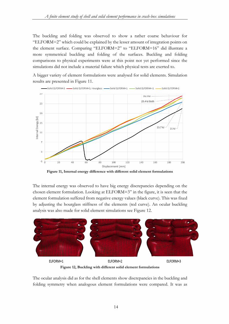
A bigger variety of element formulations were analysed for solid elements. Simulation

results are presented in Figure 11.

Figure 11, Internal energy difference with different solid element formulations

The internal energy was observed to have big energy discrepancies depending on the

chosen element formulation. Looking at ELFORM=3” in the figure, it is seen that the

element formulation suffered from negative energy values (black curve). This was fixed

by adjusting the hourglass stiffness of the elements (red curve). An ocular buckling

analysis was also made for solid element simulations see Figure 12.

Figure 12, Buckling with different solid element formulations

The ocular analysis did as for the shell elements show discrepancies in the buckling and

folding symmetry when analogous element formulations were compared. It was as


15

previously stated that the buckling and folding symmetry was dependent on the amount

of integration points on the element surface.

A result comparison was made for the element formulations to conclude the

investigation of element formulations for both shell and solid elements, see Figure 13.

Figure 13, Internal energy for shell and solid elements

It was observed that the internal energy values were grouped by a higher and a lower

value cluster. The difference in values was quite significant with a 6.4 kJ difference

between the maximum and minimum values in the graph. For the analogous element

formulations the differences were 320 J for one point integration formulation and 490

J for the fully integrated element formulation. The results were also analysed by

comparing simulation time values, see Figure 14.

Figure 14, Simulation times for shell and solid element formulations

It was observed that the simulation times were significantly longer for solid elements in

comparison to shell elements. It was however not expected that “ELFORM=16” would

be faster to simulate than “ELFORM=2” with respect to element theory, see section

20.7 kJ19.9 kJ

23.7 kJ25.4 kJ26.3 kJ

02468

10121416182022242628

0 50 100 150 200

Inte

rnal

En

ergy

[kJ

]

Displacement [mm]

Shell ELFORM=2

Shell ELFORM=16

COMPANY SIM

Solid ELFORM=-1

Solid ELFORM=1

Solid ELFORM=2

Solid ELFORM=3

01:46:30 02:01:45 02:34:09

06:36:56

17:52:22

30:16:11

34:35:09

0:00:00

12:00:00

24:00:00

36:00:00

Ho

urs


16

4.2. It is on the other hand important to note that the simulation times might vary due

to different processor efficiencies in the calculation cluster.

6.1.2 Simulation efficiency

Performing simulations with solid elements proved to not be time efficient so

simulations with different time steps were performed to investigate if the time efficiency

could be increased. The time steps were controlled by adding mass to the elements in

order to speed up the simulation times, see Appendix B for more information. Software

parameters provided by Sapa technology did include a time step value which had the

magnitude of 1e-7.

Performing simulations with different time step were considered to take too long time

when simulating solid elements, so shell elements were used to get the idea of the time

step implications on the results. With the help of equations presented in Appendix B, a

time step of the value 2.75e-7 could be achieved.

Simulations with the calculated time step were performed with increased and decreased

time steps by the factor of 10. Simulation times were observed to increase with smaller

time steps and decrease with a bigger time step, see Figure 15.

Figure 15, Simulation times with different time step values

Obtained time values below the calculated time step (marked in red) was considered to

be unstable since the calculation time did not show a steady decrease while values above

the calculated value were observed to have a steady increase.

0.23 0.05 0.20

2.58 hours with the

calculated time step value

3.91 hours with the company … 4.33 4.50

5.25

0.00

1.00

2.00

3.00

4.00

5.00

6.00

Tim

e [h

]

Time step value 2.75 multiplied with different factors


17

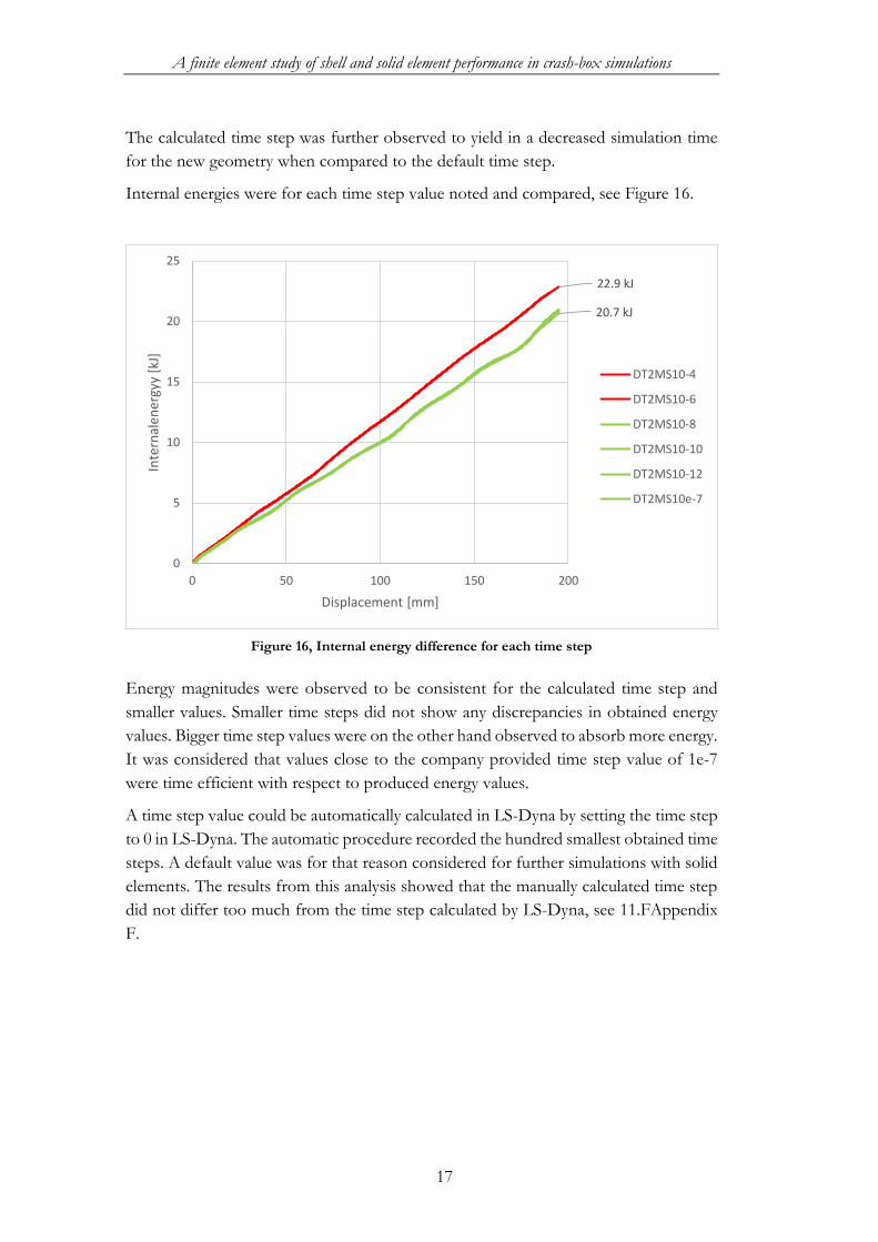
The calculated time step was further observed to yield in a decreased simulation time

for the new geometry when compared to the default time step.

Internal energies were for each time step value noted and compared, see Figure 16.

Figure 16, Internal energy difference for each time step

Energy magnitudes were observed to be consistent for the calculated time step and

smaller values. Smaller time steps did not show any discrepancies in obtained energy

values. Bigger time step values were on the other hand observed to absorb more energy.

It was considered that values close to the company provided time step value of 1e-7

were time efficient with respect to produced energy values.

A time step value could be automatically calculated in LS-Dyna by setting the time step

to 0 in LS-Dyna. The automatic procedure recorded the hundred smallest obtained time

steps. A default value was for that reason considered for further simulations with solid

elements. The results from this analysis showed that the manually calculated time step

did not differ too much from the time step calculated by LS-Dyna, see 11.FAppendix

F.

22.9 kJ

20.7 kJ

0

5

10

15

20

25

0 50 100 150 200

Inte

rnal

ener

gyy

[kJ]

Displacement [mm]

DT2MS10-4

DT2MS10-6

DT2MS10-8

DT2MS10-10

DT2MS10-12

DT2MS10e-7


18

6.2 Choice of parameters

Software parameters were with the previous step concluded chosen in LS-Dyna for

simulations with shell and solid elements. Chosen element formulations for both shell

and solid elements were the analogous formulations which are the one integration point

formulation and the fully integration formulation.

The contact type was chosen to be of the type segment based search with a master and

slave logic. The slave part was the crashed part to be crashed and the master part was

the tool.

Simulations were at this point performed with the company provided anisotropic

damage model “GISSMO” and a software integrated material failure parameter in the

isotropic material model. The damage parameters for GISSMO will not be revealed due

to a non-disclosure agreement (NDA) with Sapa technology. Simulations with material

failure were applied by setting the failure parameter to 70%, 80% and 90% of the plastic

strain. Elements that reached specified values were deleted by LS-Dyna.

The calculated time step value was chosen from the previous section in order to obtain

time efficient simulations with shell elements. A default time step value was further

chosen for simulations solid elements in order to achieve results safe from any time

step manipulations.

Internal energies and simulation times were to be measured as previously. Simulations

with the chosen software parameters were performed by the following scheme:

Simulations with shell elements in combination with GISSMO as well as a

material failure model

Simulations with solid elements in combination with a material failure model

Simulations with solid elements were only performed with a material failure model since

GISSMO was not adapted for solid elements. The result comparison for shell and solid

elements with the material failure model had the purpose to merely indicate the

difference in absorbed energy magnitudes.


19

6.3 Simulations with shell elements

Simulations with shell elements were performed with both the new geometry and the

geometry provided by the company. The material failure model was used during

simulations of both geometries with the purpose of seeing eventual result discrepancies.

Obtained results were not observed to differ in energy behaviour when compared to

each other but did differ in the energy magnitude for the new geometry, see Figure 17.

Figure 17, Simulations with material failure model for the new geometry

The highest absorbed energy occurred when most of the material was intact, in this case

with the specified value of 90% failure to plastic strain so the results were considered

to be valid. The absorbed energy was for the company provided geometry observed to

have the same energy behaviour as for the new geometry. The energy magnitudes were

further observed to be slightly larger in magnitude when compared to the new

geometry, see Figure 18 on the next page.

Figure 18, Simulations with material failure model for company geometry

Analysing both graph shows that more energy was absorbed with the mesh provided

by the company. The difference in magnitude for both geometries was 1.6 kJ for 90%,

700 J for 80% and 800 J for 70% fail to plastic strain.

16.5 kJ

17.7 kJ

19 kJ

0

2

4

6

8

10

12

14

16

18

20

0 50 100 150 200

Inte

rnal

en

ergy

[kJ

]

Displacement [mm]

New geom 70% strain[Shell]



17.3 kJ

18.4 kJ

20.6 kJ

0

3

6

9

12

15

18

21

0 50 100 150 200

Inte

rnal

En

ergy

[kJ

]

Displacement [mm]

Company 70% strain

Company 80% strain

Company 90% strain


20

Simulations with GISSMO in combination with the new geometry displayed an energy

behavior which was not by a linear nature as previous simulations were. The geometry

provided by the company did on the other hand show a consistent energy behavior

with previous simulations, see Figure 19.

Figure 19, Absorbed energy with GISSMO for both geometries

The internal energy was observed to have a linear behavior for the new geometry until

approximately 70 [mm] of displacement before starting to increase in magnitude. The

increase was further noted to accelerate at a higher rate when exceeding approximately

120 [mm] of displacement.

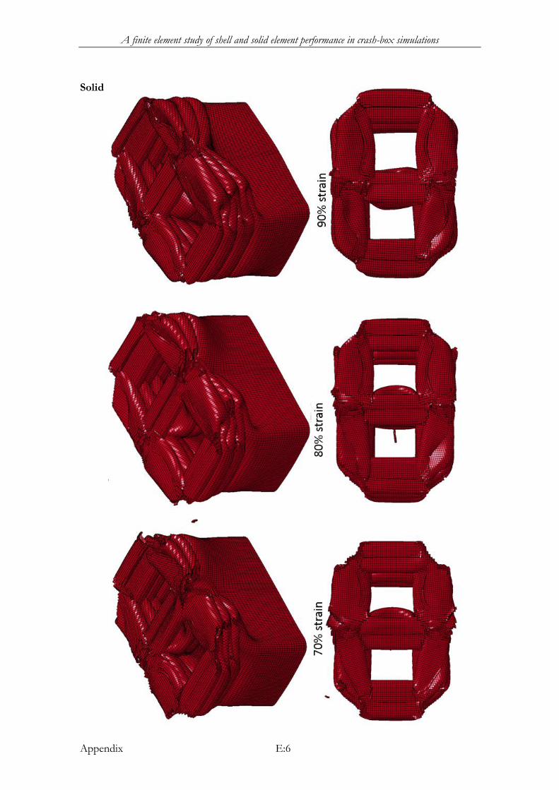
A visual comparison was made for both material models. The material failure model

showed that fewer elements were deleted with a larger failure parameter, see Figure 20.

Figure 20, Visual presentation of simulations with material failure

The deleted elements showed consistency with energy magnitudes presented in Figure

18 since deleted elements implied that eventual energy stored in the failed elements was

deleted.

GISSMO was at first sight observed to show that a large amount of elements was

deleted and was compared to previously performed simulations with a material failure

model, see Figure 21.

22.9 kJ

19.61 kJ

0

4

8

12

16

20

24

0 50 100 150 200

Inte

rnal

en

ergy

[kJ

]

Displacement [mm]

NewGeometry

CompanyGeometry


21

Figure 21, Visual comparison of GISSMO and material failure model

The visual presentation showed that GISSMO provided more wrecked models in

comparison to the material failure simulations.

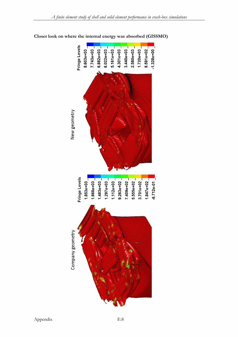
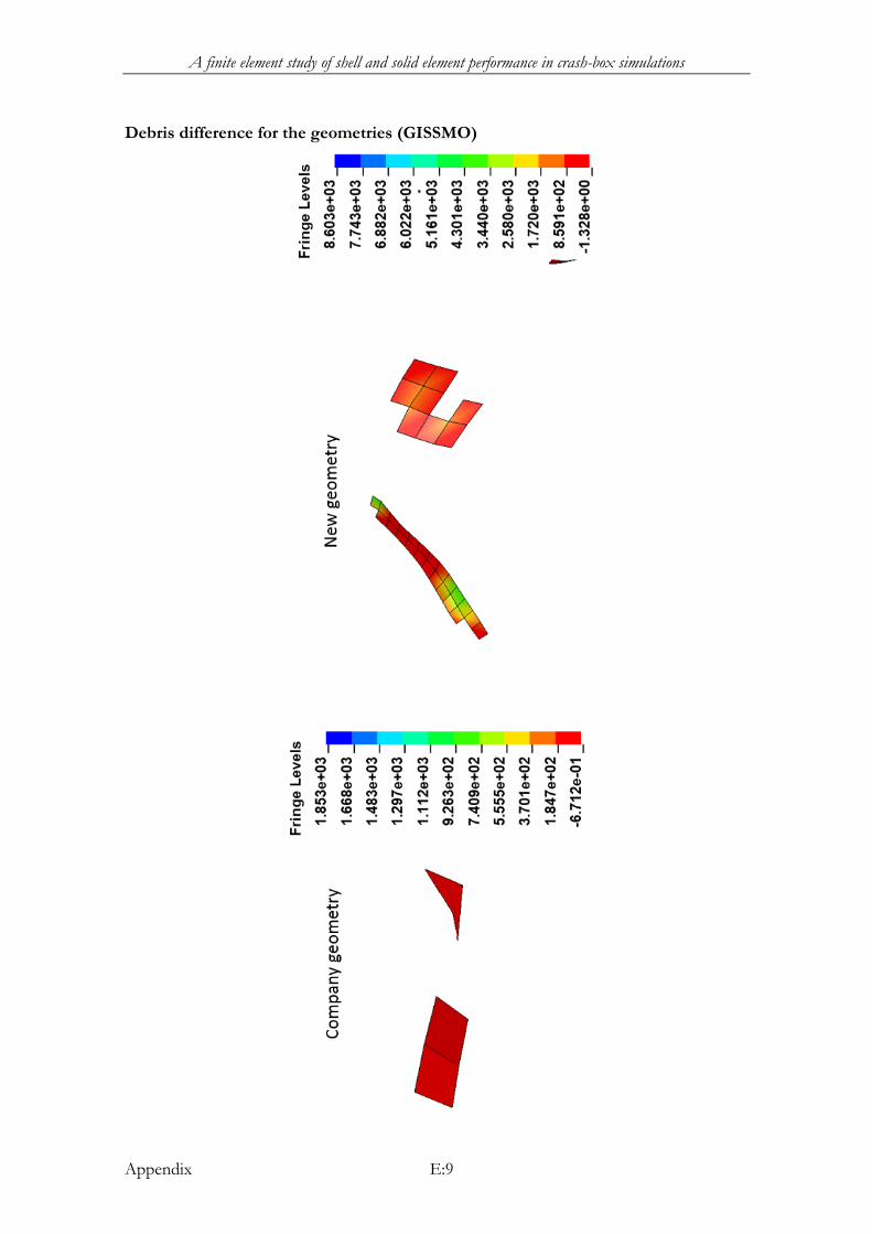
Investigating the simulated GISSMO models from a farther distance displayed that not

all elements were deleted. Debris in different sizes was observed to be scattered around

the model where energy still was absorbed, see Figure 22.

Figure 22, Debris scatter for GISSMO with and sample showing absorbed energy

Simulations with the company provided geometry did not provide debris of the same

magnitude as shown in Figure 22. The debris was further observed not to absorb any

energy for the company simulations. It was not determined if the absorbed energy in

the debris for the new geometry was excluded from the final energy values in LS-Dyna.

See Appendix H for more illustrations from this section.


22

6.4 Simulations with solid elements

Simulations with solid elements were as previously mentioned only performed with a

material failure model. The beam was observed to absorb more internal energy when

simulated with solid elements in comparison to shell elements, see Figure 23.

Figure 23, absorbed energy with Solid vs. Shell elements

It was further noted that the two analysed element types did create an upper and lower

value cluster. A visual comparison was also made of the simulated beams. The results

were as for shell elements observed to relate to the energy graph as previously by

showing that more elements were saved when a larger fail parameter was set, see Figure

24.

Figure 24, Solid elements with material failure model

Simulation times were also noted and compared for all simulations in this chapter and

can be found with other more visually detailed figures and comparisons from this entire

section in Appendix H.

23.5 kJ24.2 kJ24.8 kJ

16.5 kJ17.7 kJ19 kJ

0

5

10

15

20

25

0 50 100 150 200

Inte

rnal

en

ergy

[kJ

]

Displacement [mm]

70% strain[Solid]

80% strain[Solid]

90% strain[Solid]


23

7 Simulations with Impetus AFEA

Simulations with impetus AFEA were done in a different manner since the FE-software

offers a different set of software parameters in comparison to LS-Dyna. The element

formulations were automatically selected by Impetus with an option of changing the

polynomial order in the elements, which means that the mesh would be divided and

refined into more elements.

Simulations were for consistency reasons performed with and without the polynomial

option to analyse the differences. Sapa Technology provided parameters for a damage

model to use when performing simulations with Impetus AFEA. The damage models

in Impetus AFEA and LS-Dyna are software wise formulated in different ways. As for

GISSMO simulations in the previous chapter, the damage parameters for Impetus

AFEA will not be revealed due to the NDA. The simulations were done by the

following scheme:

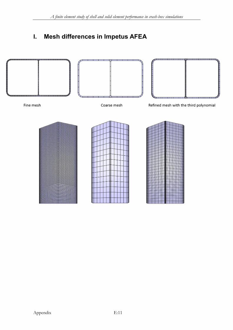
Simulations with the same fine solid mesh as used in LS-Dyna performed with

and without a damage model

Simulations with a coarse mesh to be refined with a polynomial of the third

degree, with and without a damage model

It was considered to be important to create similar input files for the both FE-software’s

in order to have a good understanding of eventual discrepancies. A series of preparatory

simulations were made with the fine mesh used in LS-Dyna where the tool failed to

reach the crushing destination so a coarser mesh was created with an element size

increased by the factor of two. The differences in the meshes used during simulations

with Impetus can be seen in Appendix 0.

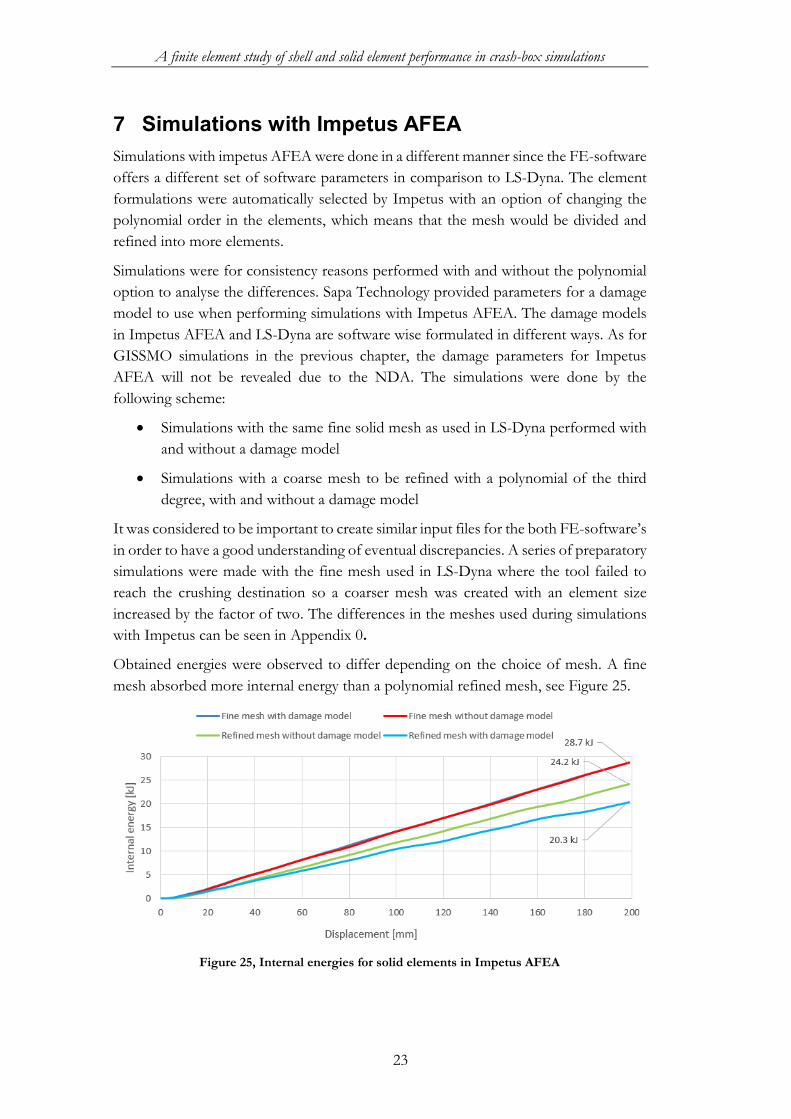
Obtained energies were observed to differ depending on the choice of mesh. A fine

mesh absorbed more internal energy than a polynomial refined mesh, see Figure 25.

Figure 25, Internal energies for solid elements in Impetus AFEA


24

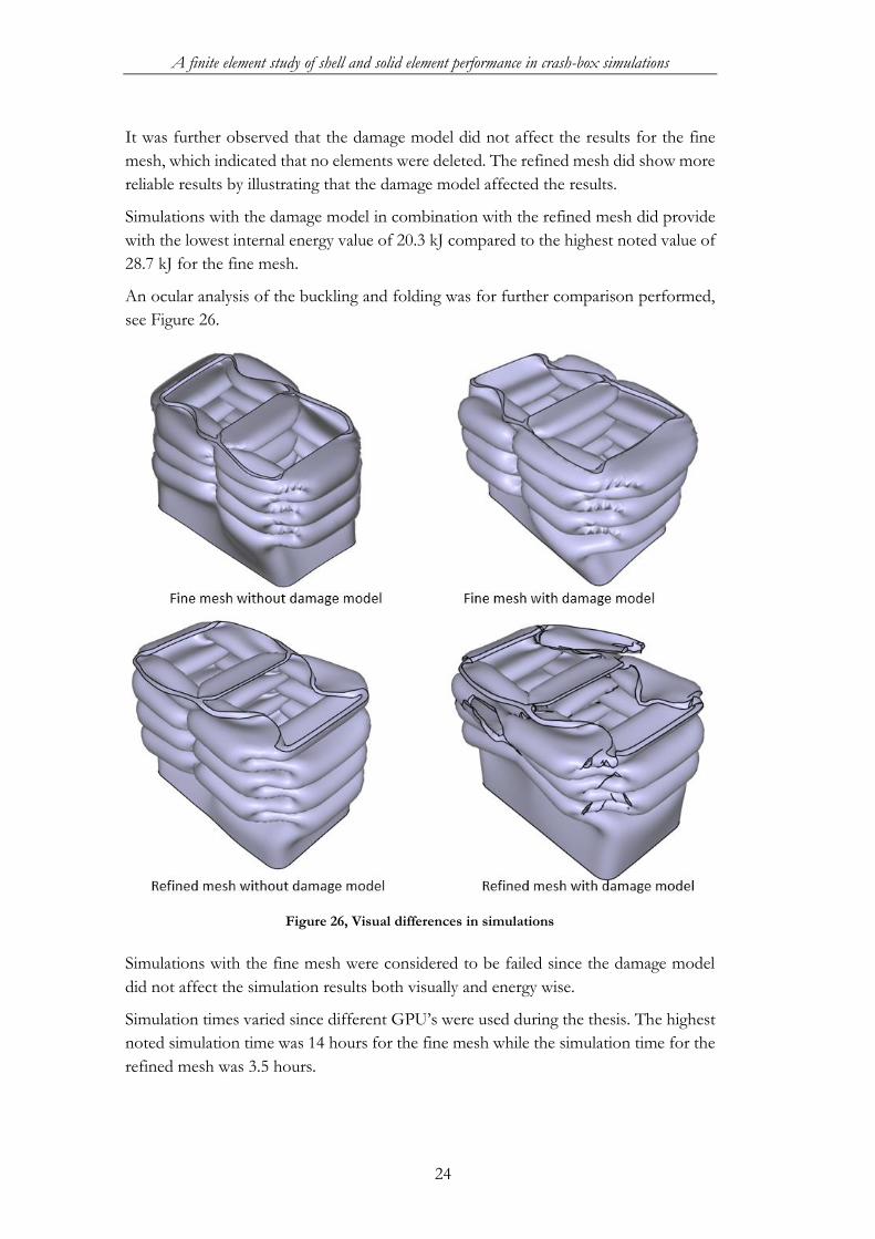
It was further observed that the damage model did not affect the results for the fine

mesh, which indicated that no elements were deleted. The refined mesh did show more

reliable results by illustrating that the damage model affected the results.

Simulations with the damage model in combination with the refined mesh did provide

with the lowest internal energy value of 20.3 kJ compared to the highest noted value of

28.7 kJ for the fine mesh.

An ocular analysis of the buckling and folding was for further comparison performed,

see Figure 26.

Figure 26, Visual differences in simulations

Simulations with the fine mesh were considered to be failed since the damage model

did not affect the simulation results both visually and energy wise.

Simulation times varied since different GPU’s were used during the thesis. The highest

noted simulation time was 14 hours for the fine mesh while the simulation time for the

refined mesh was 3.5 hours.


25

8 Further measurements

Results from simulations with the two FE-software’s were at this point collected and

measured with reference to each other and to physical tests. Energy comparisons will

be referred to the Appendix due to graph sizes.

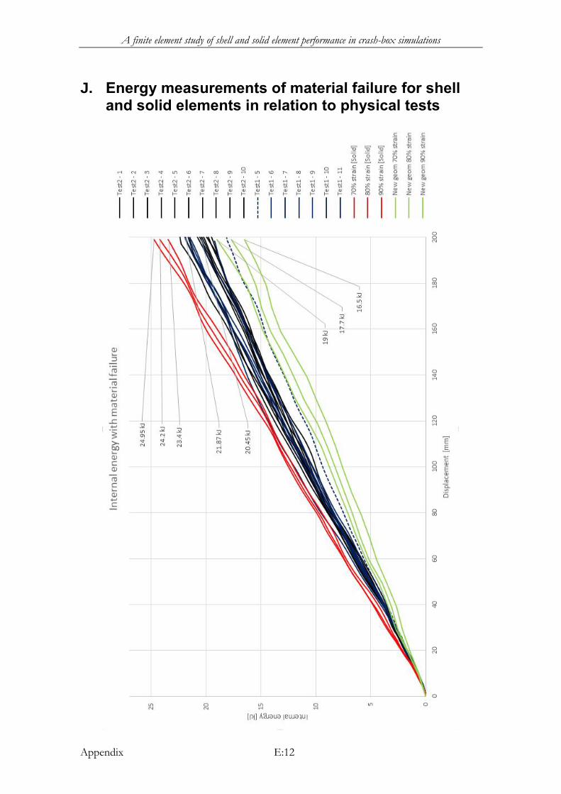
Comparing results from simulations with a material failure model for both shell and

solid elements did show that solid elements were inclined to yield in larger energy values

compared to physical tests. Shell values were noted on the other hand to yield in values

a bit lower than physical tests, see Appendix J for more information.

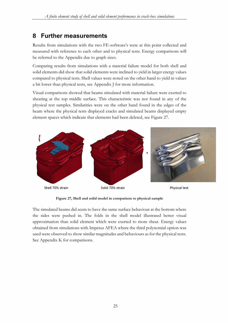
Visual comparisons showed that beams simulated with material failure were exerted to

shearing at the top middle surface. This characteristic was not found in any of the

physical test samples. Similarities were on the other hand found in the edges of the

beam where the physical tests displayed cracks and simulated beams displayed empty

element spaces which indicate that elements had been deleted, see Figure 27.

Figure 27, Shell and solid model in comparison to physical sample

The simulated beams did seem to have the same surface behaviour at the bottom where

the sides were pushed in. The folds in the shell model illustrated better visual

approximation than solid element which were exerted to more shear. Energy values

obtained from simulations with Impetus AFEA where the third polynomial option was

used were observed to show similar magnitudes and behaviours as for the physical tests.

See Appendix K for comparisons.


26

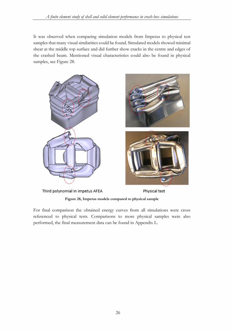
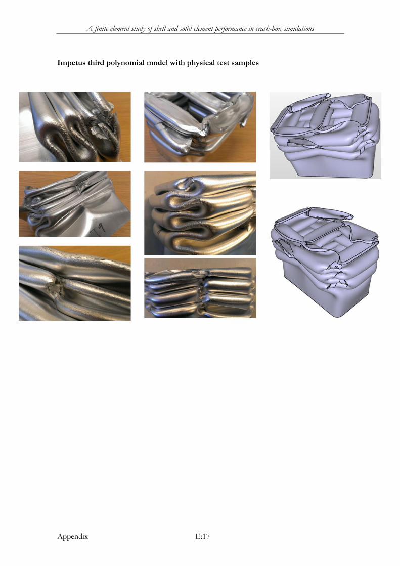
It was observed when comparing simulation models from Impetus to physical test

samples that many visual similarities could be found. Simulated models showed minimal

shear at the middle top surface and did further show cracks in the centre and edges of

the crashed beam. Mentioned visual characteristics could also be found in physical

samples, see Figure 28.

Figure 28, Impetus models compared to physical sample

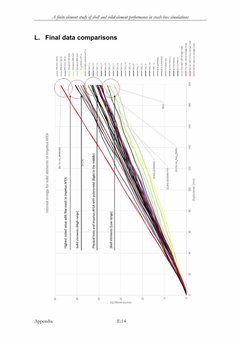
For final comparison the obtained energy curves from all simulations were cross

referenced to physical tests. Comparisons to more physical samples were also

performed, the final measurement data can be found in Appendix L.


27

9 Results

Obtained energy values from simulations with solid elements were in general higher

than values obtained from simulations with shell elements and physical test data. Shell

elements did on the other hand absorb less energy in comparison to physical tests. The

simulation times were also noted to be larger when performing simulations with solid

elements.

Results obtained from simulations with GISSMO in combination with the new

geometry were observed to have different energy behaviours during the crash when

compared to simulations with company geometry. The energy magnitude was further

noted to be larger for GISSMO when simulated with the new geometry. A characteristic

energy behaviour was noted where the energy suffered from a rapid increase in

magnitude when exceeding approximately half of the crushing distance towards the end

of the crushing destination. Simulations with material failure in combination with shell

elements did yield in energy values close to the company simulated GISSMO values but

with lower simulation times.

The internal energy was for the new geometry further observed to be larger in

magnitude during simulations without any material failure or damage model in

comparison to simulations with the company provided geometry.

Solid elements were seen to be consistent in the high magnitudes of absorbed energy

when simulated with and without a material failure model. The magnitudes did decrease

with an applied failure model.

Simulations with Impetus AFEA were not only time efficient but also provided both

visually and energy accurate results. The accuracy was as previously measured by

comparisons to physical tests. Energy behaviours did in Impetus show consistency

throughout simulations when compared to both FE-software’s. The absorbed energy

in Impetus did illustrate a linear behaviour and was as in most simulations with LS-

Dyna observed to decrease in magnitude when a damage model was applied.

Visual observations showed a shear at the top of the beam when simulated with LS-

Dyna while no visual shear was present in Impetus.


28

10 Analysis and discussion

Simulations with the new geometry in LS-Dyna were at some points cumbersome by

displaying higher absorbed energies for lower material failure parameters than for

higher failure parameters. This was considered to be odd. Applying a warping stiffness

of the elements fixed the issue but indicated at the same time that elements with

different aspect ratios in the same mesh can prove to be troublesome.

Solving the issue by applying a warping stiffness was also considered to be logical since

elongated elements are not considered to be as robust as square ones. The different

aspect ratios of the elements were also considered to be a factor for the achieved energy

behaviours when simulating GISSMO in combination with the new geometry. The

results from GISSMO simulation did also present an odd behaviour since the amount

of absorbed energy increased rapidly and exceeded other noted energy values. The

debris that was noted in the GISSMO simulation did show that energy was stored at

some locations which indicates that some optimizations might be needed in GISSMO

with the purpose of removing the excessive debris.

Simulations with solid elements showed that the absorbed energy was somewhat

overestimated by LS-Dyna. The solid elements did also take long time to simulate and

were not considered to be efficient neither in energy estimation nor in time efficiency.

Performing simulations with Impetus AFEA was considered to be much simpler due

to an updated interface and greatly reduced list of software parameters in comparison

to LS-Dyna. The input code was by the reduced software options much smaller and

could because of that be easily be altered, so eventual changes could be performed in a

fast manner.

The software provided two contact formulations where the difference wasn’t clear.

Both formulations were thereby investigated and showed quite different outcomes. The

contact formulation “Contact_super” made the beam too stiff for some reason so it

exploded. The contact formulation “Contact” resembled the formulation in LS-Dyna

by presenting the option of choosing a master and slave part. It was also the latter

contact formulation that resulted in a full simulation.

By using the third polynomial option for setting up an element formulation, a coarse

mesh could be used as input data. The FE-software recoded the mesh automatically

and simulation results were achieved fast. The simulation results did overall present a

better quality in both visual and energy aspects.

Visual comparisons did show that the element formulation in both FE-software’s is

different. The same basic geometry was used in both software’s and yet different

outcomes were achieved in which a noted shear could be present in LS-Dyna but not

in Impetus AFEA.


29

11 Conclusions and future work

The results proved that shell elements were efficient in order to provide a good

estimation of energy values with not too costly simulation times. Simulations with solid

elements were not observed to provide similar results so it is not recommend to use

solid elements for simulations with this type of profile where the walls are very thin.

Even though obtained energy magnitudes with shell elements in combination with

material failure were somewhat lower than the physical tests, the obtained results were

considered to be a good approximation indicator for absorbed energy values.

Simulation times with a material failure model were also noted to be significantly shorter

than for GISSMO.

Simulations with Impetus AFEA were observed to provide different results compared

to simulations with solid elements in LS-Dyna. The refined third polynomial elements

did not only provide good visual presentations of the crashed beams but also energy

values in the range of physical tests. It was in the end of the comparison step seen that

the visual presentations often mirrored energy data. For example, the material failure

simulations showed a direct correspondence by illustrating that more energy had been

absorbed when more elements were present. Another example would be the result

comparison between Impetus and physical tests. The visual comparison showed more

similarities to physical test samples than simulations with LS-Dyna and mirrored the

similarities to observed energy behaviours and magnitudes.

The results indicate that it is recommended to use shell elements when simulating this

geometrical type of profile with LS-Dyna. If solid elements are to be used, the

polynomial option in Impetus AFEA is recommended.

It was further considered to be important to investigate result implications when

manipulating the time step parameters even though no major discoveries were made.

The main purpose of this minor investigation was to see if differences in internal energy

values and simulation times could be obtained with larger or smaller time steps and by

doing so, decrease the simulation times. Obtained data proved that same magnitudes in

the internal energy could be achieved with smaller time steps but with the cost of

increased simulation times. The change in absorbed energy would first occur when

larger time steps were applied. This analysis was considered as an additional

investigation during the thesis work.

For future work, more simulations could be performed with different aspect ratios of

the elements in the same mesh to observe the differences for shell and solid elements,

this thesis only presented one example of different aspect ratios.

Simulations with shell elements could also be further investigated by analysing more

element formulations in LS-Dyna.


30

References

1. Wang, Erke, ANSYS, Thin-wall structure simulation (2006). [Electronic]. Available: <http://www.ansys.com/staticassets/ANSYS/staticassets/resourcelibrary/confpaper/2006-Int-ANSYS-Conf-22.pdf> [2015-03-22]

2. Olsson, Björn, Dynamore Testing of constitutive models of AA6082-TS in LS-Dyna (2014). [Electronic]. Available: <http://www.dynamore.se/en/resources/papers/2014-nordic-ls-dyna-forum-2013-presentations/testing-of-different-material-models-of-aa6082-t6> [2015-01-30]

3. Sapa Group, Sapa group Information, Company webpage (2009). [Electronic]. Available: <http://www.sapagroup.com/en/aluminium-and-rd/research--development/sapa-technology> [2015-01-30]

4. Reuters, Thomson, Concept of crashworthiness, Findlaw (2013). [Electronic] Available: <http://injury.findlaw.com/product-liability/car-defects-the-concept-of-crashworthiness.html>[2015-02-13]

5. University West (2014). Course Syllabus for mechanics of materials, advanced level [Electronic]. Available: <https://kubik.hv.se/print_courseplan.php?courseid=2989&course_rev_id=8606&lang=en> [2015-01-30]

6. University West (2014). Course Syllabus for mechanics of materials, advanced level [Electronic]. Available: <https://kubik.hv.se/print_courseplan.php?courseid=6244&course_rev_id=10413&lang=en> [2015-01-30]

7. Bala, Suri. Time integration D3view (2007). [Electronic] Available: <http://blog2.d3view.com/wp-content/uploads/2007/04/timeintegration_v1.pdf>[2015-02-13]

8. Bala, Suri. Contact definitions (2007). [Electronic] Available: <http://www.dynasupport.com/tutorial/contact-modeling-in-ls-dyna>[2015-02-13]

9. Nicklasson, Kjell (2014). Basics about FEA stapled compendium. University West.

10. Hafue, André. Schweizerhof, Karl. DuBois, Paul. Review of shell element formulatons, Dynamore (2013). [Electronic] Available: <https://www.dynamore.de/de/download/papers/2013-ls-dyna-forum/documents/review-of-shell-element-formulations-in-ls-dyna-properties-limits-advantages-disadvantages>[2015-02-01]

11. Dynamore, LS-Dyna (2014). User guide and commands for LS-Dyna [Electronic]. Available: <http://www.dynasupport.com/manuals/ls-dyna-manuals/> [2015-01-30]

http://www.dynamore.se/en/resources/papers/2014-nordic-ls-dyna-forum-2013-presentations/testing-of-different-material-models-of-aa6082-t6

http://www.dynamore.se/en/resources/papers/2014-nordic-ls-dyna-forum-2013-presentations/testing-of-different-material-models-of-aa6082-t6

http://www.sapagroup.com/en/aluminium-and-rd/research--development/sapa-technology

http://www.sapagroup.com/en/aluminium-and-rd/research--development/sapa-technology

http://injury.findlaw.com/product-liability/car-defects-the-concept-of-crashworthiness.html

http://injury.findlaw.com/product-liability/car-defects-the-concept-of-crashworthiness.html

https://kubik.hv.se/print_courseplan.php?courseid=2989&course_rev_id=8606&lang=en




http://blog2.d3view.com/wp-content/uploads/2007/04/timeintegration_v1.pdf

http://blog2.d3view.com/wp-content/uploads/2007/04/timeintegration_v1.pdf

http://www.dynasupport.com/tutorial/contact-modeling-in-ls-dyna

http://www.dynasupport.com/tutorial/contact-modeling-in-ls-dyna

https://www.dynamore.de/de/download/papers/2013-ls-dyna-forum/documents/review-of-shell-element-formulations-in-ls-dyna-properties-limits-advantages-disadvantages



http://www.dynasupport.com/manuals/ls-dyna-manuals/


Appendix A:1

A. Sapa beam


Appendix B:1

B. Time step equation

E= Young’s modulus

ρ= Specific mass density

v= Poisson

Formulas can be found in references [11] and [9].

The mass scaling manipulates the speed of sound parameters when applied. A simple

example is to understand that Newton’s second law in crash analysis is mass dependent,

and if the mass is scaled too much, the result changes.

𝑆𝑝𝑒𝑒𝑑 𝑜𝑓 𝑠𝑜𝑢𝑛𝑑 = √𝐸

𝜌(1 + 𝑣2)

𝐶𝑟𝑖𝑡𝑖𝑐𝑎𝑙 𝑡𝑖𝑚𝑒 𝑠𝑡𝑒𝑝 = 𝐸𝑙𝑒𝑚𝑒𝑛𝑡 𝐴𝑟𝑒𝑎

𝑆𝑝𝑒𝑒𝑑 𝑜𝑓 𝑠𝑜𝑢𝑛𝑑 𝑥 𝐿𝑎𝑟𝑔𝑒𝑠𝑡 𝑒𝑙𝑒𝑚𝑒𝑛𝑡 𝑙𝑒𝑛𝑔ℎ𝑡


Appendix C:1

C. Shell and solid CAD models

Shell surface to the left. Solid surface to the right.


Appendix D:1

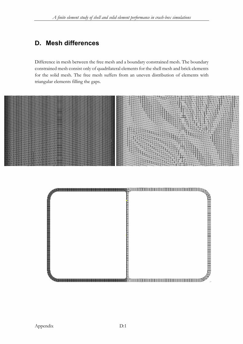
D. Mesh differences

Difference in mesh between the free mesh and a boundary constrained mesh. The boundary

constrained mesh consist only of quadrilateral elements for the shell mesh and brick elements

for the solid mesh. The free mesh suffers from an uneven distribution of elements with

triangular elements filling the gaps.


Appendix E:1

E. Initial buckling and folding observation

Comparison of buckling and folding on the crashed beams. The left beam presents the

company geometry


Appendix E:2

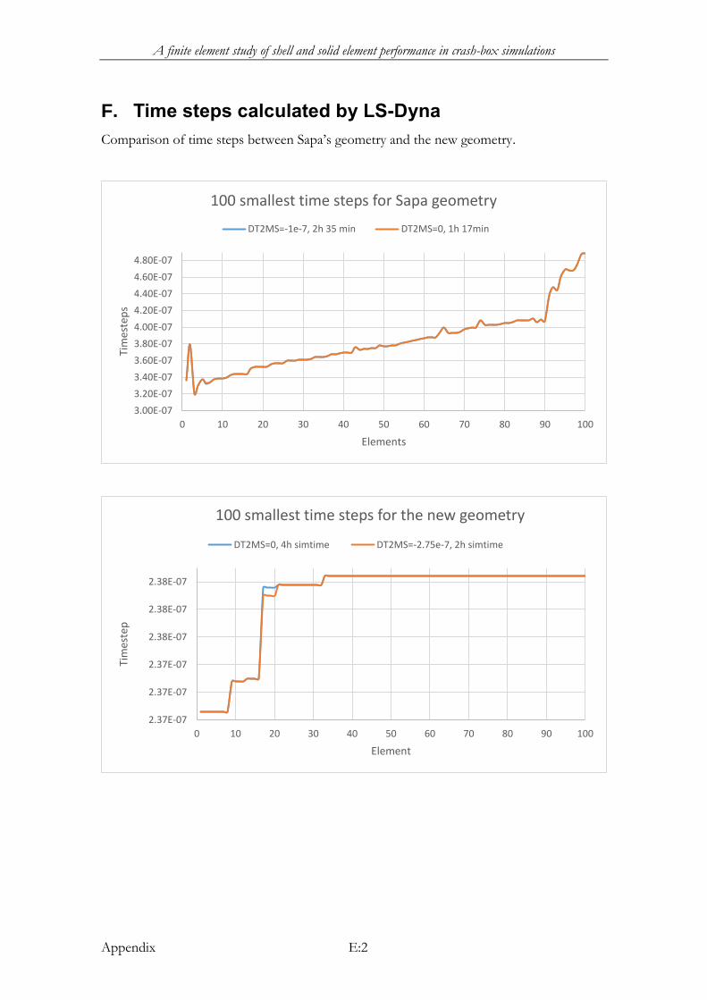
F. Time steps calculated by LS-Dyna

Comparison of time steps between Sapa’s geometry and the new geometry.

3.00E-07

3.20E-07

3.40E-07

3.60E-07

3.80E-07

4.00E-07

4.20E-07

4.40E-07

4.60E-07

4.80E-07

0 10 20 30 40 50 60 70 80 90 100

Tim

este

ps

Elements

100 smallest time steps for Sapa geometry

DT2MS=-1e-7, 2h 35 min DT2MS=0, 1h 17min

2.37E-07

2.37E-07

2.37E-07

2.38E-07

2.38E-07

2.38E-07

0 10 20 30 40 50 60 70 80 90 100

Tim

este

p

Element

100 smallest time steps for the new geometry

DT2MS=0, 4h simtime DT2MS=-2.75e-7, 2h simtime


Appendix E:3

00.

10.

20.

30.

40.

50.

60.

70.

80.

91

320

330

340

350

360

370

380

390

Stra

in [%

]

Stress [MPa]

G. Material data

Given material properties:

Mass density = 2.7e-9

Young’s modulus = 70 000 MPa

Poisson’s ratio = 0.33

Yield stress= 320 MPa

With the stress-strain curve,


Appendix E:4

H. Material failure and GISSMO (Visual, Times and Debris)

Shell


Appendix E:5

GISSMO


Appendix E:6

Solid


Appendix E:7

Fringe level comparison for both geometries (GISSMO)


Appendix E:8

Closer look on where the internal energy was absorbed (GISSMO)


Appendix E:9

Debris difference for the geometries (GISSMO)


Appendix E:10

Simulation times with material failure and GISSMO (New geometry only)


Appendix E:11

I. Mesh differences in Impetus AFEA


Appendix E:12

J. Energy measurements of material failure for shell and solid elements in relation to physical tests


Appendix E:13

K. Energy comparisons for Impetus AFEA and physical tests


Appendix E:14

L. Final data comparisons


Appendix E:15

Model comparison between FE-software’s


Appendix E:16

Physical test samples and simulated models with material failure


Appendix E:17

Impetus third polynomial model with physical test samples

A finite element study of shell and solid element performance in …808638/FULLTEXT01.pdf · A...

Documents

Transcript of A finite element study of shell and solid element performance in …808638/FULLTEXT01.pdf · A...